Embed Size (px)
Citation preview

A non-parametric approach for setting safety stocklevels
John P. Saldanha, Bradley S. PriceJohn Chambers College of Business & Economics, West Virginia University, Morgantown, WV 26506
[email protected], [email protected]
Douglas J. ThomasDarden School of Business, University of Virginia, Charlottesville, VA 22903
In practice, lead time demand (LTD) can be non-standard: skewed, multi-modal or highly variable; factors
that compromise the validity of the classic approaches for setting safety stock levels. Motivated by encoun-
tering this problem at our industry partner, we develop an approach for setting safety stock levels using
the bootstrap, a widely-used statistical procedure. We extend prior research that has used the bootstrap
for quantile estimation to address the multi-parameter estimation of safety stocks. We develop a multi-
variate central limit theorem for the bootstrap mean and bootstrap quantile – components of the safety
stock calculation – highlighting why the generalization of these bootstrap methods is critical for inventory
management. These results provide a theoretical underpinning for the bootstrap estimator of safety stock
and permit the construction of confidence intervals for safety stock estimates, allowing decision makers to
understand the reliability with which the desired service level will be achieved. Building on our theoretical
results, and supported by numerical experiments, we provide insights on the behavior of the bootstrap for
various LTD distributions, which our results demonstrate are critical when employing the bootstrap method.
Implementation results with our industry partner indicate our approach is quite effective in setting safety
stock levels.
Key words : Inventory management, safety stocks, non-parametric, bootstrap, continuous review
History : June 11, 2020
1. Introduction
Setting appropriate safety stock levels is an important decision for firms in many industries. As
global sourcing continues to grow (Rose and Reeves 2017, Torsekar 2018), firms face long and
variable lead times, potentially making safety stock decisions more important and more difficult.
The textbook approach to setting safety stocks assumes that lead time demand (LTD) follows a
known distribution (e.g., normal), but it is well documented that lead time demand can be skewed,
multi-modal or highly variable (Tyworth and O’Neill 1997, Vernimmen et al. 2008). When these
factors are present, and compromise the validity of distributional assumptions, classic textbook
1
Electronic copy available at: https://ssrn.com/abstract=3624998

Saldanha, Price, Thomas: A non-parametric approach for setting safety stock levels2 Article submitted to Operations Research; manuscript no.
approaches may produce poor results (Das et al. 2014). This is precisely the problem we encoun-
tered at our industry partner (MakerCo) where lead time demands were not well represented with
standard distributions and attempts to apply classic approaches were unsuccessful.
This paper describes the development and implementation of our data-driven, non-parametric
approach to setting safety stocks based on the bootstrap. While our work on this problem was
motivated by conditions at MakerCo, our approach is general and can be implemented without
modification in other settings. There are both theoretical and methodological contributions of
our work, as the statistical theory for the safety stock estimator, and the bootstrap safety stock
estimator have not been developed or explored in the literature.
1.1. Setting safety stocks at MakerCo
MakerCo is a large firm that manufactures several thousand discrete, limited shelf-life products in
manufacturing facilities globally. Several of these products rank among the highest selling products
in their category in several global markets. In this study, we worked on a small set of high-value,
limited shelf-life raw materials, each of which is used in the production of a single finished product
at a single production facility in North America. These materials are sourced from international
suppliers where limited production capacity from batch manufacturing campaigns and unreliable
transit times contribute to long, stochastic lead times that frequently exhibit left- or right-skew and
multi-modality. In addition, MakerCo experiences volatility in the demand for finished products,
and thus the dependent raw material demand. While management typically aims for a four-month
fence to freeze production, the reality is that changes within this horizon are frequently made, with
one manager noting the four-month fence is “a ‘slushy’ period due to the volatile demand in the
industry and the need to be flexible” (email communication with procurement manager). Inspection
of the finished goods demand and forecasting data confirmed that demand distributions are non-
standard, forecast errors were non-normal, and forecast accuracy is poor, with mean absolute
percentage error (MAPE) >50%. The stochasticity of lead time and demand combine to result in
LTD distributions that are skewed and multi-modal. Figure 1 shows estimated LTD distributions
for two of MakerCo’s raw materials.
The underlying non-standard nature of the LTD distribution means that the classic approaches
built into most ERP systems (Das et al. 2014), including that used by MakerCo, failed to provide
safety stock estimates that met the desired service level within the limits of the target inventory
investment. Confronted with inconsistent estimates produced by the classic approaches in the ERP
systems, managers resorted to alternate solutions. In the absence of any guidance of how to balance
service and cost when faced with irregular LTD distributions, these alternate solutions involve
elaborate yet imprecise computations that lead to sub-optimal results maximizing one metric (e.g.,
Electronic copy available at: https://ssrn.com/abstract=3624998


Saldanha, Price, Thomas: A non-parametric approach for setting safety stock levels4 Article submitted to Operations Research; manuscript no.
underlying lead-time demand process and led to poor results. High inventory levels of some products
took up valuable warehouse space and resulted in obsolescence and expensive material write-offs.
Low inventories resulted in frequent stockouts of critical raw materials that delayed customer
fulfillment incurring expensive failure-to-supply penalties. Additionally, the baseline approach was
lengthy, requiring 40 hours of analyst time to review and set safety stocks. Consequently, this was
typically done every quarter. Hence, MakerCo opted to work with the research team to develop and
implement the non-parametric approach to set safety stocks for a small set of 9 key raw materials.
These are all classified as A-items: high-volume, high-value, and high-impact if there is a failure to
supply.
1.2. The Bootstrap Approach
We estimate safety stocks directly from empirical lead time and demand data. This builds on
the work of Bookbinder and Lordahl (1989), Lordahl and Bookbinder (1994) and Fricker and
Goodhart (2000). These previous approaches estimate reorder points for the continuous review
control policies with a probability of no stockout (PNS) service criterion (Bijvank 2014) where LTD
data potentially follows non-standard distributions. Estimation of the reorder point using bootstrap
is equivalent to estimating a quantile, which is a typical application for bootstrap methods. In this
work we generalize these approaches to multi-parameter inventory estimators, specifically safety
stock. Through our theory development and numerical experiments we demonstrate that accounting
for the correlation structure between the sample mean and the sample quantile produces a better
estimator of safety stock.
We ground our method in bootstrap theory and develop central limit theorems for the bootstrap
estimator of safety stock. Our theoretical results establish that safety stock must be bootstrapped
directly from empirical LTD. This explicates the validity of the bootstrap approach to estimate
safety stocks from an empirical LTD mixture of observed empirical lead time and demand data. This
contribution is particularly salient as many popular ERP software, including those encountered by
the authors in their field work, require operations managers to enter safety stocks to set materials’
inventory policies.
We employ controlled simulation experiments to provide insights on appropriate tuning param-
eters for the bootstrap approach, and the behavior of the bootstrap estimator of safety stock
compared to classic approaches. We demonstrate that ignoring proper tuning of the bootstrap
parameters can potentially compromise the reliability of the safety stock estimates. We also demon-
strate that when LTD takes non-standard distribution forms the bootstrap out performs alternative
approaches. In the case of standard distributions as the number of lead time cycles increases the
bootstrap begins to outperform alternative approaches that make heavy distributional assumptions.
Electronic copy available at: https://ssrn.com/abstract=3624998

Saldanha, Price, Thomas: A non-parametric approach for setting safety stock levelsArticle submitted to Operations Research; manuscript no. 5
The controlled simulation results establish appropriate tuning parameters and provide evidence
that our approach works well for non-standard LTD distributions such as those observed at Mak-
erCo. These results motivated a simulation study based on MakerCo data. The results of this
simulation study were critical in the research teams’ engagement with MakerCo as a means of
securing managers’ trust in the bootstrap approach by using the organization’s own data to rig-
orously test the proposed approach. Based on the MakerCo simulation results, the procurement
planning team began a pilot of the bootstrap method in the second quarter of 2018. Since then,
comparisons of the bootstrap approach relative to the baseline approach indicate the potential for
significant reductions in safety stocks without sacrificing service levels. Our controlled and industry
simulation experiments along with the pilot implementation results provide a compelling case for
supply chain managers encountering similar replenishment lead-time and demand conditions to
estimate bootstrap safety stocks and corresponding confidence intervals directly from their ERP
systems’ empirical lead-time and demand data.
The remainder of the paper is organized as follows, in Section 2, we discuss the relevant literature
and position our contribution. In Section 3 we present the bootstrap central limit theorems that
provide the theoretical justification for our approach. In Section 4 we present our controlled numer-
ical experiments allowing us to compare the performance of our bootstrap approach to optimal
benchmarks, which are of course not identifiable in our industry use case. In Section 5, we describe
our simulation using MakerCo data, the results of which led to the pilot implementation. Results
from the pilot implementation are reported in Section 5.3. We conclude with a discussion of our
contributions to the literature and the mainstream practice of inventory management in Section 6;
highlighting areas where the bootstrap is appropriate and where it is limited in setting inventory
policies with potential areas for future research.
2. Literature Review
We focus our discussion around the two main approaches in the literature for dealing with non-
standard LTD: the compound distribution approach, where different distributions, including mix-
tures, are used to represent LTD; and, distribution-free approaches. The bootstrap approach we
propose in this article is a non-parametric approach that falls under the distribution-free literature.
2.1. Compound Distribution Approach
The classic compound distribution approach popular in the literature and practice follows the
seminal works of Fetter and Dalleck (1961) and Hadley andWhitin (1963). This approach, assuming
a known underlying distribution of LTD, suffers from three well-documented flaws. First, in practice
LTD data are rarely tracked by firms’ information systems and are rarely known or observed
Electronic copy available at: https://ssrn.com/abstract=3624998

Saldanha, Price, Thomas: A non-parametric approach for setting safety stock levels6 Article submitted to Operations Research; manuscript no.
(Rossetti and Unlu 2011, Silver et al. 2016). Instead, for mathematical tractability we assume
the unobserved probability distribution of LTD follows some known form. In cases where LTD
are observed we can evaluate the fit of the empirical data and use an appropriate probability
distribution. Even if LTD are tracked, in cases of seasonal demand and non-normal forecast errors
(Eppen and Martin 1988), the textbook methods would fall short. Second, compound-distribution
approaches typically assume standard LTD distributions, while LTD distributions can often exhibit
high coefficients of variance, right skew and multi-modality (Das et al. 2014, Tyworth and O’Neill
1997, Vernimmen et al. 2008). In practice we observe right-skew, multi-modal and generally non-
standard distributional forms for the LTD component distributions of demand (Bachman et al.
2016, Zhang et al. 2014), and lead time (Das et al. 2014, Saldanha et al. 2009), which result in
non-standard distributional forms of LTD (Mentzer and Krishnan 1985, Tyworth and O’Neill 1997,
Saldanha and Swan 2017). Third, operations managers often have to work with small sample sizes
of lead time and/or demand to set inventory parameters that may lead to significant errors in
estimation for both compound distribution approaches (Bai et al. 2012, Silver and Rahnama 1986),
and data-driven bootstrap approaches (Bookbinder and Lordahl 1989, Efron and Tibshirani 1986).
The compound distribution approach that enjoys widespread use is the normal distribution,
primarily because of its ease of use. However, incorrectly assuming LTD is normally distributed
introduces significant errors in inventory policy decisions and costs (Das et al. 2014, Eppen and
Martin 1988, Mentzer and Krishnan 1985), and can result in a significant cost penalty from the vio-
lation of the normality assumption of LTD (Lau and Lau 2003). Consequently, several alternatives
have been proposed to the normal , notably the gamma distribution (Keaton 1995, Turrini and
Meissner 2019, Tyworth et al. 1996, Vernimmen et al. 2008) the Erlang distribution, a special case
of the gamma (Kim et al. 2004, Leven and Segerstedt 2004), the Weibull, the lognormal (Tadika-
malla 1984), and the negative binomial (Shore 1986). However, similar to the normal approach,
all of these approaches suffer when the LTD distribution realized in practice does not follow the
underlying distributional assumption.
Other approaches include the use of a mixture of truncated exponentials (MTE) to estimate
reorder points when demand has normal, gamma or lognormal distribution that rely on complex
statistical routines to fit empirical data (Cobb 2013, Cobb et al. 2015). Tyworth (1992) employs
a convex combination of conditional normal probability distributions of demand erected over a
range of discrete lead time values. Keaton (1995) extends this approach to include conditional
gamma probability distributions of demand. However, the true underlying demand distributions
are typically unknown and assuming specific demand distributions to estimate inventory control
parameters can be problematic (Bai et al. 2012).
Electronic copy available at: https://ssrn.com/abstract=3624998
Saldanha, Price, Thomas: A non-parametric approach for setting safety stock levelsArticle submitted to Operations Research; manuscript no. 7
Rossetti and Unlu (2011) propose a workaround to these problems when LTD is unknown employ-
ing a set of rules for selecting the most appropriate distribution of LTD based on the distributions of
lead time and demand.These rules are predicated on LTD data conforming to a standard unimodal
distributional form and do not accommodate non-standard multi-modal LTD distributions often
found in practice (Bachman et al. 2016, Bookbinder and Lordahl 1989, Das et al. 2014, Eppen and
Martin 1988, Fricker and Goodhart 2000, Zhang et al. 2014). Also, we know that the distributions
of demand (Bachman et al. 2016, Cattani et al. 2011) and lead time (Das et al. 2014, Saldanha
et al. 2009) rarely follow standard distributional forms.
All these compound-distribution approaches involve an intermediate step estimating the
moments of some combination of lead time, demand and LTD to arrive at the safety stockand
thus run counter to the Main Principle of Inference (Vapnik 2013). Distribution-free or non-
parametric approaches are worthy of investigation as candidate approaches for setting safety stocks
directly from empirical lead time and demand data. Next, we turn to distribution-free, data-driven
approaches.
2.2. Distribution-Free Approaches
Distribution-free approaches preclude the need to determine the distributional form of lead-time,
demand, or LTD. We have seen such approaches employed for single-period newsvendor settings
with limited historical demand data (Akcay et al. 2011, Huh et al. 2011, Levi et al. 2015, 2007,
Saghafian and Tomlin 2016). Notably, Ramamurthy et al. (2012) invoke Vapnik’s Main Principle
of Inference to employ a data-driven approach employing operational statistics to estimate the
optimal policy for the newsvendor model. More recently Ban and Rudin (2019) investigated using
a data-driven approach to the newsvendor problem using machine learning algorithms based on
high dimensional quantile regression. Similarly, Cao and Shen (2019) extend a time-series quantile
estimation approach to determine replenishment strategies for the newsvendor problem. Huber
et al. (2019) demonstrate that such data-driven machine learning approaches that employ quantile
regression perform well with large data-sets.
Following Yano (1985), there is a stream of literature on distribution-free min-max, continuous-
review integrated inventory modeling approaches (cf. Gutgutia and Jha 2018, Moon et al. 2014,
Tajbakhsh 2010). The distribution-free nature relies on the assumption that the distribution of
LTD can be constructed using a mixture model where the LTD mixture of the component dis-
tributions of lead time and demand has a finite mean and variance. However, variances must be
equal between components and the means and variances must conform to a specific relationship.
In addition, these methods assume fixed lead times and, are computationally intense often relying
Electronic copy available at: https://ssrn.com/abstract=3624998

Saldanha, Price, Thomas: A non-parametric approach for setting safety stock levels8 Article submitted to Operations Research; manuscript no.
on iterative algorithms to estimate the distributional functions of LTD to obtain estimates of the
mean, variance, and mixture proportions.
Bachman et al. (2016) develop a specialized aggregate inventory policy for the United States
Defense Logistics Agency (US DLA) to manage inventory assuming replenishment lead times are
fixed, for items that face either frequent highly-variable demand or infrequent demand, in group-
ings or portfolios. Inventory decisions for items in each portfolio are estimated according to a
continuous review inventory policy. Besides being computationally intensive and necessitating a
multi-step iterative solution method involving simulations, the Bachman et al. (2016) approaches
are tailored to US DLA settings that assumes fixed lead times. Zhang et al. (2014) also develop a
specialized approach for managing Kroger Pharmacies’ drug inventories. Their approach is similarly
computationally-involved necessitating a multi-step approach including simulations and assumes
lead times are fixed.
Application of the bootstrap approach to estimate inventory in not new. Hasni et al. (2019)
review the literature on bootstrapping demand forecasts to manage spare parts inventories. Similar
to Zhou and Viswanathan (2011), the work in this literature stream assumes fixed lead times. As we
have mentioned earlier, lead-time distributions encountered in practice are frequently non-standard
(Das et al. 2014, Saldanha et al. 2009), which results in non-standard distributional forms of LTD
(Mentzer and Krishnan 1985, Tyworth and O’Neill 1997, Saldanha and Swan 2017).
Bookbinder and Lordahl (1989) were the first to propose the bootstrap method to estimate
quantiles from the empirical non-standard LTD distribution corresponding to different levels of
PNS, or P1 service level, to set reorder points (ROP) for the (s,Q) policy.Consistent with bootstrap
theory (Efron and Tibshirani 1986), Bookbinder and Lordahl (1989) prove that the consistency
and unbiasedness of the bootstrap estimates increases with the bootstrap sample size (m) and
the number of bootstrap resamples (B) for the sample quantile. Wang and Rao (1992) extend the
bootstrap approach to estimate the ROP quantiles from empirical LTD data when demand follows
an AR(1) process. Fricker and Goodhart (2000) build on the (Fetter and Dalleck 1961, p. 52) Monte
Carlo method extending the Bookbinder and Lordahl (1989) approach to bootstrap an empirical
mixture of LTD from empirical lead time and demand data to directly estimate the reorder point
in the singular setting of the U.S. Marine Corps’ Expeditionary Force’s local “retail” inventories.
While they introduce the concept of bootstrapping an empirical mixture of LTD from empirical
lead time and demand data to estimate the ROP from the quantile defined by the PNS .
These works are important because they show the applicability of the bootstrap in an inventory
setting, but only investigate the estimation of the reorder point, which is equivalent to estimating
a quantile of a distribution. These works do not provide methodological or theoretical guidance
on how multi-parameter inventory control parameters, such as safety stock, should be estimated.
Electronic copy available at: https://ssrn.com/abstract=3624998
Saldanha, Price, Thomas: A non-parametric approach for setting safety stock levelsArticle submitted to Operations Research; manuscript no. 9
As our focus is on safety stock, which we argue is an essential inventory control policy input to
many popular ERP systems, our work provides an example of the generalization of the methodol-
ogy proposed by Bookbinder and Lordahl (1989) and Fricker and Goodhart (2000). Furthermore,
we provide theoretical justification for the bootstrap estimation of safety stock using asymptotic
statistical theory that shows a non-negligible covariance between the sample mean and sample
quantile, the components of the safety stock calculation.
3. Bootstrap Theory for Estimating Safety Stocks
3.1. Methodology
Since logistics information systems and ERP systems typically do not directly capture LTD data
(Das et al. 2014), managers must use lead time data and demand data that are not paired. Even if a
system would directly capture LTD data, when lead-times and demands are highly variable, viewing
these data as separate offers managers some flexibility in specifying the input data. For instance,
it could be beneficial to supplement demand data with forecasts of demands to accommodate
market volatility. With this compound distribution framework in mind we define the lead time
data li , i= 1, . . . , nL as independent realizations of the random variable L, which has mean µL and
variance σ2L. Similarly we assume the demand data dj, j = 1, . . . , nD as independent realizations
of the random variable D, which has mean µD and variance σ2D. We also assume that L and D
are independent random variables. Finally assume, though it is never observed directly in our
framework, LTD is generated from the random variable X which has mean µX and variance σ2X .
Under the compound distribution framework for LTD discussed in Section 2.1 the estimates of the
mean and variance of lead time (µL , σ2L) and, the estimates of the mean and variance of demand
(µD, σ2D) are used to estimate the mean of LTD µX = µLµD and its variance σ2
X = µLσ2D+ µ2
Dσ2L. Our
focus is on the estimation of the safety stock, which is defined in the familiar way as SS = τ −µX
where τ = F−1X (P1) such that F−1
X is the inverse cumulative distribution function (CDF) of X.
For example, the safety stock estimate under the normal distribution assumption is calculated as
SS = F−1Z (P1)σX , where F−1
Z (·) is the CDF of the random variable Z ∼ N(0,1) for a P1 service
level.
As we consider a bootstrap under the compound-distribution framework, an issue arises when
considering the bootstrap sample size (m), which would typically be the number of observations
in the sample of LTD, which in this case is unknown because a random sample of LTD is not
observed directly. We present results from a a simulation study in Appendix C to justify the
choice of bootstrap sample size as m = nL. This choice matches intuition under the compound
distribution framework as the number of observed lead time demands correspond to the number of
observed lead times. The previous guidance provided by Fricker and Goodhart (2000) is m=B or
Electronic copy available at: https://ssrn.com/abstract=3624998

Saldanha, Price, Thomas: A non-parametric approach for setting safety stock levels10 Article submitted to Operations Research; manuscript no.
the bootstrap sample size equals the bootstrap re-samples, which we demonstrate (Appendix C)
results in significantly biased estimates.
To obtain the bootstrap estimates of safety stock we first generate the bootstrap samples under
the compound distribution framework, and then directly estimate safety stock for each bootstrap
sample. More explicitly, we construct the b-th bootstrap sample of LTD, x(b)1 , . . . , x(b)
nLsuch that
the ith observation is x(b)i =
∑lij=1 dj, where each li is randomly selected with replacement from
l1, . . . , lnL, and each dj, j = 1, ..., li is randomly selected with replacement from d1, . . . , dn
D. We
repeat this procedure B times to construct B bootstrap samples. We propose calculating the
bootstrap safety stock as SS∗
=B−1∑B
b=1 SS(b), where SS(b) = Y (b)−n−1
L
∑nL
i=1 x(b)i , is the estimate
of safety stock for the b-th bootstrap sample such that Y (b) is the P1-th quantile for the b-th
bootstrap sample.
Using methods proposed by the extant literature that bootstrap only the reorder point either
directly from LTD data (Bookbinder and Lordahl 1989), or from a mixture of LTD (Fricker and
Goodhart 2000), one could estimate safety stock using a second method. Given the bootstrap
quantile Y ∗ is the estimate for the reorder point at a given PNS, safety stock can be calculated as
SS = Y ∗ − µX where µX = µLµD is the empirical estimate of the mean of LTD. Our results in the
next section indicate that this procedure ignores relevant information: the covariance between the
estimates of the mean and quantile.
3.2. Theoretical Results
In this section, we show there exists a central limit theorem for safety stock and bootstrap of
safety stock when LTD is known, both of which have a non-negligible covariance structure that is
computationally intractable without heavy distributional assumptions. This shows that calculating
the safety stock for each bootstrap sample, as we propose, will account for this covariance structure.
In Appendix A we provide some insights on how the re-sampling technique we propose is actually
generating a distribution under the assumption that L and D are independent.
To formulate the asymptotic results, consider the setting where LTD can be observed directly.
Consider x1, . . . , xn as the sample of lead time demands akin to the bootstrap setting in Bookbinder
and Lordahl (1989). The distributions of both the sample mean and sample quantile are known,
and the joint asymptotic properties were explored by Lin and Wu (1980) and Ferguson (1998).
Though the joint distribution of the sample mean and sample median was discovered by Laplace
well before this work. We restate this critical result from Ferguson (1998) here in the context of
LTD as it is central to our discussion of safety stock.
Theorem 1. Let x1, . . . , xn, the observed LTD, be random draws from a random variable, X,
with distribution function FX(x), density fX(x), mean µ, variance σ2, and empirical distribution
Electronic copy available at: https://ssrn.com/abstract=3624998

Saldanha, Price, Thomas: A non-parametric approach for setting safety stock levelsArticle submitted to Operations Research; manuscript no. 11
function Fn(x). Let 0 < p < 1 so that FX(τp) = p. Assume fX(x) is continuous and positive at
F−1X (p). Let Fn(Yp) = p, and
x=n∑
i=1
xi/n
then
√n
((xYp
)−(µτp
))L−→N2
(00
),
σ2x
κ(p)
fx(F−1
X(p))
κ(p)
fX (F−1
X(p))
p(1−p)
f2
X(F−1
X(p))
where κ(p) =E(Lp(X,F−1
X (p))), such that Lp(z, a) = p(z− a)I(z ≥ a)+ (1− p)(z− a)I(a< z).
We omit the proof and refer the reader to Section 5 of Ferguson (1998) for the full discussion
of the proof. Instead, we provide a brief outline of the proof here as the concepts are important
to our understanding of the bootstrapping of safety stocks; a multivariate estimator. The proof
uses the Bahadur representation of the sample mean and sample quantile, and the convergence
of each distribution to a distinct Brownian bridge. From there the Cramer-Wold device shows
that the limiting distribution is jointly normal. Finally, the covariances are calculated between
the two resulting Brownian bridges, and converge to what is shown above. It is of note that this
asymptotic covariance term is non-zero if κ(p) 6= 0. Ferguson (1998) describes this as the minimum
p-th deviation around F−1X (p). To our knowledge, this work is the first in the inventory literature
to point out this multivariate central limit theorem. Next, we extend Theorem 1 directly to obtain
a central limit theorem for safety stock.
Corollary 1. Define safety stock as
SS = Yp − x.
Given the assumptions and definitions in Theorem 1, safety stock has the asymptotic distribution
√n(SS−F−1
X (p)+µ)
L−→N(0, σ2ss),
where σ2ss = σ2
X + p(1−p)
f2
X(F−1
x (p))− 2 κ(p)
fX (F−1
X(p))
.
We omit the proof as this is just a linear transformation of the joint distribution in Theorem 1.
As Cramer-Wold was used in the proof for Theorem 1 this is just a direct consequence.
The results of Theorem 1 show the asymptotic covariance between the sample mean and sample
quantile is non-zero and could be considered intractable for non-standard distributions of LTD.
Thus, the bootstrap could be used to create confidence intervals on safety stock in general settings.
Even if the distributions are standard, the covariance terms that include the quantity κ(p) are
Electronic copy available at: https://ssrn.com/abstract=3624998

Saldanha, Price, Thomas: A non-parametric approach for setting safety stock levels12 Article submitted to Operations Research; manuscript no.
still difficult to calculate directly, making bootstrap estimation an attractive alternative. Moreover,
the asymptotic properties of the bootstrap estimates of sample quantities are known and well
understood using Bickel and Freedman (1981), but the joint asymptotic properties of the bootstrap
mean and bootstrap quantiles have not been investigated. In this case we need to combine the
concepts of both techniques to define the joint distribution of the sample mean and sample quantile,
and therefore, the distribution of the bootstrap of safety stock. Again we will present this theorem
in the context of LTD.
Theorem 2. Given the assumptions and definitions of Theorem 1, also assume FX is twice differ-
entiable at the p− th quantile. Let x∗
1, . . . , x∗
n represent a bootstrap sample of size n (sampling with
replacement) from the sample of lead time demands x1, . . . , xn. Define the empirical distribution
function of the bootstrap sample as Gn such that Gn(Y∗
p ) = p. Finally define x∗ = n−1∑n
i=1 x∗
i , then
along almost all sample sequences and as n tends to infinity,
√n
((x∗
Y ∗
p
)−(xYp
))L−→N2
(00
),
σ2x
κ(p)
fX (F−1
X(p))
κ(p)
fX (F−1
X(p))
p(1−p)
fX (F−1
X(p))
We relegate a more detailed proof of Theorem 2 to Appendix B of the e-companion for this
manuscript. Notice the asymptotic covariance is the same as presented in Theorem 1. The signif-
icance of this result is the multivariate normality of the estimators, and the ability to explicitly
state the covariance structure. We next extend this result directly to safety stock.
Corollary 2. Assume the settings detailed in Theorem 2 hold, then
√n(Y ∗
p − x∗ − SS)
L−→N(0, σ2ss)
Again the proof of the corollary follows directly from Theorem 2 as the Cramer-Wold device is
used in the proof.
The theorems and corollaries introduced in this section give theoretical justification for the boot-
strap approach we propose for safety stock.The asymptotic covariance matrices from Theorems 1
and 2 shows that there is a non-negligible relationship between the two statistics that yield safety
stock. When safety stock is calculated directly for each bootstrap sample, then the covariance
structure for each bootstrap sample is maintained and a sampling distribution of the statistic is
preserved enabling the estimation of bootstrap confidence intervals for safety stock. Should the two
quantities be bootstrapped independently and difference of estimates taken, then the covariance
structure is ignored, and the information of the sampling distribution is lost. Corollaries 1 and 2
provide the transformation directly to the safety stock calculation, which show how that covariance
structure plays a role in the variance of safety stock. To our knowledge this is the first work to
Electronic copy available at: https://ssrn.com/abstract=3624998

Saldanha, Price, Thomas: A non-parametric approach for setting safety stock levelsArticle submitted to Operations Research; manuscript no. 13
explicitly define the variance of safety stock and suggest the distribution of safety stocks be inves-
tigated. With this in mind, the variance component required for inference is difficult to calculate,
meaning in practice whether LTD is observed or in a compound distribution setting, the bootstrap
procedure for safety stock is an attractive procedure for estimation (Efron and Tibshirani 1986).
Next, we present a set of numerical experiments where we evaluate our approach, and the classic
approach comprised of the commonly used normal and gamma approaches, against optimal bench-
marks. The results of these experiments demonstrate the performance of the bootstrap approach
relative to the classic approaches for estimating safety stocks and minimizing inventory costs under
different replenishment conditions represented by standard and non-standard LTD distributions.
4. Numerical Experiments
Our numerical experiments compare the bootstrap approach and two classic textbook compound
distributional approaches (normal and gamma) to an optimal benchmark. As shown in Figure 1,
we encounter multi-modal LTD distributions at MakerCo, but we also want to investigate how our
approach works for unimodal distributions. Thus, in our experiments, we consider both unimodal
and bimodal lead time distributions. For unimodal lead times, we employ lognormal distributions
as described in Table 1. These lead-time distributions include regular bell-shaped to non-standard
right skew. For bimodal lead times we vary the mixture ratio (π) of the left and right modes to yield
left- and right-skew distributions (Table 2). For all experiments we employ a single gamma demand
distribution with a CV = 0.2 that allow us to represent the non-standard LTD distributions using
only the skew and bimodality of the lead time distributions.
Table 1 Unimodal lead time distributions used to generate lead time demand.
Distribution Mean CV SkewLognormal 5 0.1 0.30Lognormal 5 0.4 1.26Lognormal 5 0.7 2.44Lognormal 25 0.1 0.30Lognormal 25 0.4 1.26Lognormal 25 0.7 2.44
Note. Distribution of demand is fixed as a gamma distribution with µ= 100 and σ= 20.
4.1. Safety Stocks
We calculate the safety stock levels assuming complete backordering, comparing the safety stock
calculated by the bootstrap, and normal and gamma methods to the optimal safety stock for every
experiment level. The quantile estimate Y ∗(b) of each bootstrap sample (b) is calculated using
Electronic copy available at: https://ssrn.com/abstract=3624998

Saldanha, Price, Thomas: A non-parametric approach for setting safety stock levels14 Article submitted to Operations Research; manuscript no.
Table 2 Component distributions of the bimodal lead time distributions used to generate the mixture of lead
time demand.
Mean CV Skew π µL1 σL1 µL2 σL2
5 0.34 -1.18 0.2 1.8 0.4 5.8 0.65 0.9 1.53 0.8 2.8 0.56 13.86 1.3925 0.34 -1.19 0.2 9 1.8 29 2.925 0.9 1.52 0.8 13.93 2.79 69.3 6.93
Note. Component distribution 1 of the bimodal lead time distribution is gamma with the α and
β parameters taken as α= µ2/σ2 and β = σ2/µ, and distribution 2 of the bimodal distribution
is normal. Distribution of demand is fixed as a gamma distribution with µ= 100 and σ= 20.
both the rank quantile estimator and the SV3 estimator for right-tailed quantiles (Sfakianakis and
Verginis 2008). These two quantiles represent a limited sample of the quantile estimators available
and allow us to control for the effects of the bootstrap method under different settings. The normal
safety stock is estimated as SSN = F−1Z (P1) · σX and the gamma safety stock is estimated as
SSN = F−1Γ (P1)− µX .
From the results of bootstrap tuning parameter experiments reported in Appendix C we see that
m= nL and B = 1,000 provides the best results. Hence, we set the levels of nL = 6, 12, 24, 50, 100.
We set nD = nL, 2nL as it is reasonable to assume that the sample size of demand will be either as
large or larger than the sample size of lead time. We considered 40 levels of PNS (P1 = 60%–99%),
yielding 2,400 experiments for the unimodal case and 1,600 experiments for the bimodal case.
The experiments are run in R version 3.5.2 on a Unix system in a high performance computing
cluster with 100 replications using fixed random seeds to ensure reproducibility. Safety stock is
calculated using all four methods (normal, gamma, bootstrap with rank quantile, bootstrap with
SV3 quantile) for each replication, which is a combination of a lead-time distribution and a level
of nL, nD and PNS. We analyze this complete set of experimental results using classification trees
with recursive partitioning methodology to identify when each of the methods yielded the best
result. The results of these analyses are available in Appendix A. Those results generally support
use of our approach when lead times are bimodal, and performance differences between methods
are small for unimodal lead time distributions. We explore these findings in Tables 3 and 4 which
show MAPE from optimal safety stock values for a subset of the experiments for a unimodal lead
time case (Table 3) and a bimodal lead time case (Table 4).
For the unimodal lead-time case shown in Table 3, we see that for almost all experiments reported,
setting safety stocks by using the gamma distribution to represent lead-time demand provides
the lowest MAPE. However, based on the 100 replications in our experiments, the mean absolute
deviations from optimal safety stock with gamma are rarely lower in a statistically significant way
Electronic copy available at: https://ssrn.com/abstract=3624998

Saldanha, Price, Thomas: A non-parametric approach for setting safety stock levelsArticle submitted to Operations Research; manuscript no. 15
as compared to bootstrap approaches. (Statistical tests are one-way ANOVAs comparing MAD
from optimal safety stock across methods.) For the bimodal lead-time case shown in Table 4, we
see that the bootstrap approaches outperform normal and gamma approaches except for P1 values
between 70%-80%. When LTD is multi-modal, for certain values of P1, the ideal safety stock value
will specify a reorder point that is in-between modes of LTD. Figure 2 corresponds to Table 4, and
it is around this value of P1 = 75% where the normal and gamma CDFs happen to intersect with
the true bimodal CDF. We note two things regarding this phenomenon. First, a manager will not
know a priori when a unimodal approach would have the good fortune to intersect the true multi-
modal LTD distribution at the desired service level. Second, as we will see in the next subsection,
the expected holding and backorder cost as a function of the reorder point is very flat in-between
modes; thus, large deviations from optimal safety stock may translate to small deviations from
optimal cost.
Table 3 Mean Absolute Percent Error from optimal safety stocks for unimodal lead time, lognormal
µ= 5,CVL = 0.4 with bootstrap approaches using B = 1,000 resamples. The lowest MAPE value for each
experiment is in bold. Cells are shaded if mean absolute deviations from optimal safety stock are not statistically
significantly different from the method with the lowest MAD.
Method nL 60% 65% 70% 75% 80% 85% 90% 95% 99% Median
True Safety Stock 12.87 40.29 70.74 105.34 146.19 197.32 266.90 383.46 650.45
Boot-R
ank 6 123% 37% 30% 32% 35% 37% 41% 49% 65% 37%
10 136% 44% 30% 27% 26% 27% 30% 36% 53% 30%24 113% 40% 27% 23% 22% 20% 20% 22% 36% 23%50 103% 34% 21% 17% 16% 14% 13% 13% 24% 17%100 71% 24% 15% 12% 10% 10% 8% 10% 16% 12%
Boot-SV3
6 131% 49% 38% 36% 37% 39% 43% 50% 65% 43%10 109% 36% 26% 24% 25% 27% 30% 36% 53% 30%24 100% 34% 24% 20% 19% 18% 18% 21% 36% 21%50 95% 31% 19% 16% 15% 13% 12% 13% 23% 16%100 70% 23% 14% 11% 10% 9% 8% 9% 16% 11%
Gam
ma
6 74% 27% 27% 28% 30% 31% 32% 34% 37% 31%10 78% 28% 23% 23% 24% 24% 25% 26% 29% 25%24 83% 28% 20% 18% 17% 17% 17% 18% 20% 18%50 85% 30% 18% 14% 12% 12% 12% 12% 14% 14%100 87% 31% 19% 14% 12% 10% 9% 9% 11% 12%
Normal
6 276% 85% 50% 39% 34% 32% 32% 34% 39% 39%10 289% 89% 49% 35% 29% 26% 25% 27% 34% 34%24 291% 90% 48% 30% 22% 18% 17% 20% 29% 29%50 301% 95% 51% 31% 19% 13% 11% 15% 27% 27%100 307% 98% 53% 32% 19% 11% 8% 12% 26% 26%
4.2. Inventory and Backorder Costs
Using the safety stock values from the experiments in the previous subsection, we investigate the
expected holding and backorder cost implications of deviations from optimal safety stock values.
Electronic copy available at: https://ssrn.com/abstract=3624998

Saldanha, Price, Thomas: A non-parametric approach for setting safety stock levels16 Article submitted to Operations Research; manuscript no.
Table 4 Mean Absolute Percent Error from optimal safety stocks for bimodal lead time,
µ= 25,CVL = 0.34, π= 0.2 with bootstrap approaches using B = 1,000 resamples. The lowest MAPE value for each
experiment is in bold. Cells are shaded if mean absolute deviations from optimal safety stock are not statistically
significantly different from the method with the lowest MAD.
Method nL 60% 65% 70% 75% 80% 85% 90% 95% 99% Median
True Safety Stock 397.75 446.69 496.61 549.55 607.37 673.55 756.08 876.78 1099.85
Boot-R
ank 6 39% 35% 34% 35% 36% 35% 34% 35% 40% 35%
10 29% 30% 30% 29% 28% 27% 27% 27% 33% 29%24 25% 24% 23% 21% 21% 20% 19% 18% 22% 21%50 19% 18% 17% 16% 15% 14% 13% 12% 14% 15%100 12% 11% 10% 9% 9% 8% 7% 7% 8% 9%
Boot-SV3
6 77% 59% 45% 36% 33% 33% 34% 35% 40% 36%10 43% 31% 28% 27% 27% 26% 26% 27% 33% 27%24 23% 23% 22% 21% 20% 19% 19% 18% 22% 21%50 19% 18% 17% 16% 14% 13% 13% 12% 14% 14%100 12% 11% 10% 9% 9% 8% 7% 7% 7% 9%
Gam
ma
6 76% 53% 33% 25% 34% 50% 67% 91% 131% 53%10 73% 50% 31% 17% 23% 36% 54% 78% 117% 50%24 71% 48% 28% 12% 17% 30% 47% 72% 111% 47%50 70% 48% 28% 10% 12% 28% 47% 73% 113% 47%
100 70% 47% 27% 8% 11% 28% 49% 74% 115% 47%
Normal
6 48% 32% 29% 34% 43% 52% 62% 74% 90% 48%10 48% 30% 20% 22% 28% 38% 49% 62% 80% 38%24 47% 29% 15% 15% 22% 31% 42% 56% 75% 31%50 47% 28% 12% 10% 18% 29% 42% 57% 76% 29%
100 46% 27% 11% 7% 17% 30% 43% 58% 78% 30%
Figure 2 The cumulative distribution functions comparing the true left skew bimodal distribution with µL = 25
and CVL = 0.34 (blue dashed line) with the normal (red) and gamma (black)
Lead Time Demands
For a given choice of P1, we set the under-stocking cost (cost of a unit backorder) to be cu = P1 and
the over-stocking cost (cost of carrying one unit of inventory for the time between replenishment
cycles) to be co = (1−P1). These costs are thus consistent with P1 = cu/(cu+ co) being the optimal
service level choice.
We carry through the two examples from the previous section and present cost results for one
unimodal case (Table 5) and one bimodal case (Table 6). For each case, we use the true, underlying
Electronic copy available at: https://ssrn.com/abstract=3624998

Saldanha, Price, Thomas: A non-parametric approach for setting safety stock levelsArticle submitted to Operations Research; manuscript no. 17
LTD distribution, specified in the previous subsection, to evaluate expected holding and backorder
cost for the reorder points implied by each calculated safety stock value. This expected cost is then
compared to the optimal expected cost.
For the unimodal case, recall from Table 3, we saw the gamma approach provide the best safety
stock values with bootstrap approaches not too far behind, often not different in a statistically
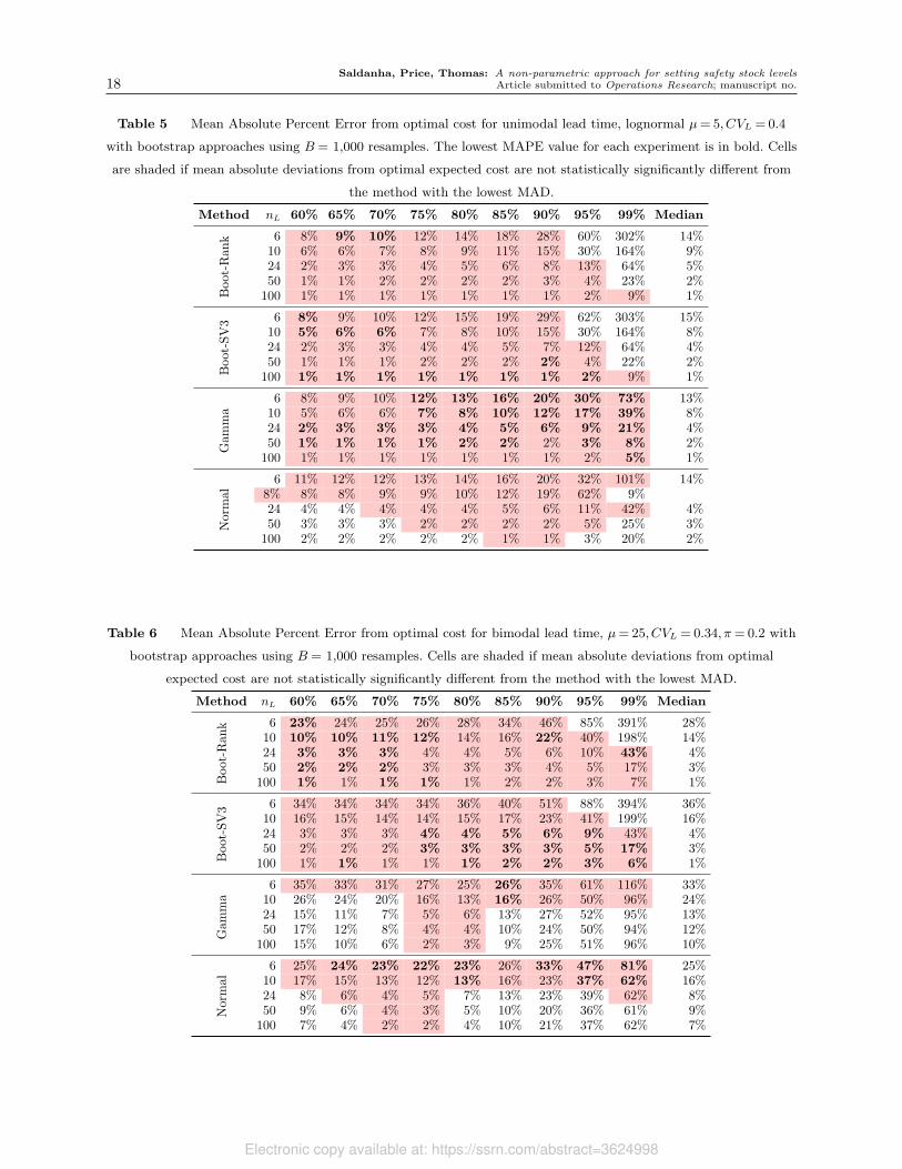
significant sense. This pattern carries through to expected cost results shown in Table 5. One
point that emerges, or is at least emphasized, in the cost results is that the data-driven bootstrap
approach suffers for small amounts of data and high quantile values (e.g., nL ≤ 10, P1 ≥ 95%).
This suggests that firms with limited data, very high target service levels, and unimodal LTD
distributions may not be well-served with non-parametric, data-driven approaches.
The better safety stock estimates produced by the bootstrap approaches for the bimodal lead-
time case shown in Table 4 also carry through to the cost results shown in Table 6. Similar to
the unimodal cost results, we see large cost deviations for limited data and very high service
levels. Recall from the previous section that the normal and gamma approaches resulted in lower
deviations from optimal safety stock for service level values near 75% due to the CDFs for those
distributions intersecting with the true LTD distribution at those values (Figure 2). As indicated
in Table 6, those better safety stock estimates do not translate to substantial cost savings since
the cost function is relatively flat between modes.
Results from these controlled experiments demonstrate that our proposed bootstrap approach
is competitive with classic approaches when lead time demand distributions are unimodal (Tables
3 and 5), and can provide better performance when LTD distributions are multi-modal (Table 4
and 6). This suggests that our approach may work well for the multi-modal LTD distributions
we observe for MakerCo (Figure 1). The results of these controlled experiments provided the
impetus for the MakerCo procurement planning team to provide the organizational data necessary
to rigorously test the proposed bootstrap approach for their own raw materials replenishment
inventories in a discrete-event simulation. In the next section, we describe this simulation study
and its results that eventually led the MakerCo management team to run a pilot implementation.
Results from the pilot implementation are also described in the next section.
5. Industry Application
To gain organizational acceptance for implementation at MakerCo, we sought to validate the
bootstrap beyond the known distributional settings studied in Section 4. To do this, we simulated
the firm’s raw materials’ replenishment operation. MakerCo operates a continuous review (s,Q)
with order quantities (Q) determined by minimum-order-quantities set by the supplier or the
frequency of MakerCo’s production needs. MakerCo management aimed for a service level of P1 =
Electronic copy available at: https://ssrn.com/abstract=3624998
Saldanha, Price, Thomas: A non-parametric approach for setting safety stock levels18 Article submitted to Operations Research; manuscript no.
Table 5 Mean Absolute Percent Error from optimal cost for unimodal lead time, lognormal µ= 5,CVL = 0.4
with bootstrap approaches using B = 1,000 resamples. The lowest MAPE value for each experiment is in bold. Cells
are shaded if mean absolute deviations from optimal expected cost are not statistically significantly different from
the method with the lowest MAD.
Method nL 60% 65% 70% 75% 80% 85% 90% 95% 99% MedianBoot-R
ank 6 8% 9% 10% 12% 14% 18% 28% 60% 302% 14%
10 6% 6% 7% 8% 9% 11% 15% 30% 164% 9%24 2% 3% 3% 4% 5% 6% 8% 13% 64% 5%50 1% 1% 2% 2% 2% 2% 3% 4% 23% 2%
100 1% 1% 1% 1% 1% 1% 1% 2% 9% 1%
Boot-SV3 6 8% 9% 10% 12% 15% 19% 29% 62% 303% 15%
10 5% 6% 6% 7% 8% 10% 15% 30% 164% 8%24 2% 3% 3% 4% 4% 5% 7% 12% 64% 4%50 1% 1% 1% 2% 2% 2% 2% 4% 22% 2%
100 1% 1% 1% 1% 1% 1% 1% 2% 9% 1%
Gam
ma
6 8% 9% 10% 12% 13% 16% 20% 30% 73% 13%10 5% 6% 6% 7% 8% 10% 12% 17% 39% 8%24 2% 3% 3% 3% 4% 5% 6% 9% 21% 4%50 1% 1% 1% 1% 2% 2% 2% 3% 8% 2%100 1% 1% 1% 1% 1% 1% 1% 2% 5% 1%
Normal
6 11% 12% 12% 13% 14% 16% 20% 32% 101% 14%8% 8% 8% 9% 9% 10% 12% 19% 62% 9%24 4% 4% 4% 4% 4% 5% 6% 11% 42% 4%50 3% 3% 3% 2% 2% 2% 2% 5% 25% 3%
100 2% 2% 2% 2% 2% 1% 1% 3% 20% 2%
Table 6 Mean Absolute Percent Error from optimal cost for bimodal lead time, µ= 25,CVL = 0.34, π= 0.2 with
bootstrap approaches using B = 1,000 resamples. Cells are shaded if mean absolute deviations from optimal
expected cost are not statistically significantly different from the method with the lowest MAD.
Method nL 60% 65% 70% 75% 80% 85% 90% 95% 99% Median
Boot-R
ank 6 23% 24% 25% 26% 28% 34% 46% 85% 391% 28%
10 10% 10% 11% 12% 14% 16% 22% 40% 198% 14%24 3% 3% 3% 4% 4% 5% 6% 10% 43% 4%50 2% 2% 2% 3% 3% 3% 4% 5% 17% 3%
100 1% 1% 1% 1% 1% 2% 2% 3% 7% 1%
Boot-SV3 6 34% 34% 34% 34% 36% 40% 51% 88% 394% 36%
10 16% 15% 14% 14% 15% 17% 23% 41% 199% 16%24 3% 3% 3% 4% 4% 5% 6% 9% 43% 4%50 2% 2% 2% 3% 3% 3% 3% 5% 17% 3%100 1% 1% 1% 1% 1% 2% 2% 3% 6% 1%
Gamma
6 35% 33% 31% 27% 25% 26% 35% 61% 116% 33%10 26% 24% 20% 16% 13% 16% 26% 50% 96% 24%24 15% 11% 7% 5% 6% 13% 27% 52% 95% 13%50 17% 12% 8% 4% 4% 10% 24% 50% 94% 12%
100 15% 10% 6% 2% 3% 9% 25% 51% 96% 10%
Norm
al
6 25% 24% 23% 22% 23% 26% 33% 47% 81% 25%10 17% 15% 13% 12% 13% 16% 23% 37% 62% 16%24 8% 6% 4% 5% 7% 13% 23% 39% 62% 8%50 9% 6% 4% 3% 5% 10% 20% 36% 61% 9%100 7% 4% 2% 2% 4% 10% 21% 37% 62% 7%
Electronic copy available at: https://ssrn.com/abstract=3624998

Saldanha, Price, Thomas: A non-parametric approach for setting safety stock levelsArticle submitted to Operations Research; manuscript no. 19
95%. Using the baseline approach, safety stocks are manually calculated in a spreadsheet and
entered into the inventory module of the ERP system that would use the fixed preset supplier lead
times to set the ROP. Raw material replenishment decisions are made continuously to maintain
sufficient safety stocks depending upon the production usage. In case of stockouts any unmet
demand due to production shortfalls is backordered.
5.1. Simulation Model
We worked with MakerCo to collect data for 9 raw material SKUs. Lead time data were collected
from each SKU’s ordering history. For the demand data we used the parent finished good’s historic
demand as there is a one-to-one relationship between finished goods and the raw materials in this
study. As the lead time and demand did not conform to any standard distributional forms we
employed empirical histograms for each of these inputs to the simulation. Baseline safety stocks
along with the resulting reorder points were used from the firm’s operations (Appendix D Table
EC.3 ). For each SKU a benchmark LTD distribution was compiled from the empirical lead time
and empirical demand data using a Monte-Carlo simulation with one million draws. These bench-
mark distributions are provided in Appendix D Figure EC.1. From these “true” benchmark LTD
distributions we compute the benchmark safety stock for the desired P1 = 95% and other LTD
statistics for each SKU, which we use to check the internal logic of the simulation model as well
as use for later comparisons.
Each simulated day, observed demand is fulfilled from available inventory, the unfilled portion
of demand is backordered. A replenishment order of fixed quantity Q is placed when the inventory
position (on-hand inventory and orders outstanding) is less than or equal to the reorder point. At
the end of each simulated day inventory and order records are updated. Three identical discrete-
event simulations of the firm’s daily inbound raw material replenishment inventory management
process run in parallel in Simul8 R© Professional Version 23. One simulation replicated MakerCo’s
extant inventory operations (baseline), a second simulated the use of the bootstrap method to set
inventory policies (bootstrap), and the third used the gamma approach to set inventory policies
(gamma). A limited experimental frame was set using three levels each of nL = 6, 10, 24 and
nD = 6, 10, 24 corresponding to the data availability defined by the firms’ operations managers.
Each experiment ran for 20 replications yielding a total of 320 runs for each method and SKU
combination. The baseline, bootstrap and gamma simulations ran in parallel, warming up for a
period of 25 years and running for 10 years. The baseline, bootstrap or gamma inputs are calculated
after the warmup period employing the historic nL and nD values collected by the end of the warm-
up period. The inventory policies by each approach are updated every 30 days reflecting MakerCo’s
practice. A single random draw of daily demand is used by all three simulations running in parallel.
Electronic copy available at: https://ssrn.com/abstract=3624998

Saldanha, Price, Thomas: A non-parametric approach for setting safety stock levels20 Article submitted to Operations Research; manuscript no.
An order is triggered separately by each of the three simulations for which a lead time value is
randomly drawn from the lead time distribution of the SKU for which the inventory process is
being simulated. Thereby, the difference in safety stocks, realized PNS and total inventory costs
(holding and backorder) is only due to the inventory estimates used and comparable across the
three approaches.
5.1.1. Model Validation To ensure the internal logic of the simulation we ran 20 replications
of the simulation warming up for a period of 25 years and running for 25 years for all 9 SKUs.
Accurate LTD data is an outcome of the correct functioning of the simulation and is critical
for correctly setting the inventory policies therein. The LTD statistics simulation output can be
compared with that of the benchmark LTD distribution statistics run independently in the Monte-
Carlo simulation. Hence, we use t-tests to compare the simulated LTD mean and standard deviation
from the three methods for each SKU with the benchmark LTD mean and standard deviation.
The comparisons use t-test confidence intervals for the mean deviation (MD) of each simulated
LTD statistic from the benchmark value shown in Appendix D Table EC.4. The results confirm
that in virtually all cases the simulated data are not significantly different from the benchmark.
An exception is for average LTD for SKU 16, which is still close to the benchmark.
To ensure the simulation was satisfactorily modeling MakerCo’s process for managing inbound
raw material replenishment inventories we met several times with the management team and pro-
vided graphical output of the simulated inventory system for each SKU, represented by the inven-
tory balance on hand, inventory position and backorders. The graphs of the simulated inventory
system allowed the management team to identify the symptoms they encountered particularly with
SKUs that posed a management challenge. For example, in Appendix D Figure EC.2, we provide
examples where the operations managers were able to identify problems with chronic overages and
underages for SKU 3 and 17, respectively. This validation offers some confidence that the simu-
lation model is internally valid and satisfactorily models the firm’s replenishment and inventory
operation.
5.2. MakerCo Simulation Results
The results of the 320 runs were used to conduct 9 one way ANOVAs for each SKU, one for each
nL and nD combination. We use the mean absolute deviation (MAD) of each method’s safety stock
estimator from that of the benchmark as the response variable and the method as the predictor. For
each ANOVA we conduct multiple pairwise comparisons of each method’s MAD by constructing
confidence intervals using the Bonferroni correction for multiple t-test comparisons. We compile
the results of these analyses in Table 7 where we show the MAD of each method’s average safety
Electronic copy available at: https://ssrn.com/abstract=3624998

Saldanha, Price, Thomas: A non-parametric approach for setting safety stock levelsArticle submitted to Operations Research; manuscript no. 21
stock from the benchmark shown as a percentage of the true safety stock for each nL and nD
combination. For each experiment we highlight the lowest MAD with bold font and color the cell
where the difference of that cell’s MAD from the lowest MAD is not statistically significant at
the α = 0.05 level. In order to visually represent settings where each method’s estimate is not
statistically different from the benchmark we sort the results by method, nL and nD.
Table 7 Results of the 9 one-way ANOVAs for each of the 9 SKUs comparing the estimators of the bootstrap,
gamma and baseline as the percentage mean absolute deviation (MAD) from the benchmark. (Lowest MAD for each
experiment in bold. Cell is colored if MAD is lowest or if MAD is not statistically significantly different than lowest.)
Method nL nD SKU3 SKU6 SKU7 SKU9 SKU10 SKU13 SKU14 SKU16 SKU17 Avg %age Diff
Bootstrap
6
6 33% 28% 42% 26% 15% 26% 44% 47% 43% 34%10 32% 30% 47% 15% 18% 32% 44% 51% 50% 35%24 37% 31% 49% 20% 19% 40% 50% 49% 54% 39%
10
6 9% 11% 23% 40% 18% 7% 22% 22% 18% 19%10 11% 13% 27% 25% 13% 10% 24% 26% 25% 19%24 14% 14% 26% 14% 12% 17% 24% 25% 32% 20%
24
6 9% 11% 11% 62% 41% 19% 10% 8% 16% 21%10 8% 9% 8% 41% 22% 11% 10% 9% 7% 14%24 4% 10% 7% 19% 20% 5% 11% 10% 4% 10%
Gamma
6
6 31% 16% 9% 91% 51% 26% 14% 13% 13% 29%10 29% 14% 13% 74% 40% 14% 12% 10% 14% 25%24 21% 11% 14% 43% 31% 9% 16% 13% 20% 20%
10
6 37% 18% 8% 84% 58% 35% 13% 7% 6% 30%10 35% 18% 6% 71% 41% 23% 12% 8% 10% 25%24 30% 15% 7% 54% 30% 14% 13% 6% 17% 21%
24
6 42% 21% 6% 88% 61% 44% 15% 8% 12% 33%10 41% 19% 6% 72% 37% 31% 13% 7% 6% 26%24 35% 18% 5% 48% 35% 23% 14% 8% 7% 21%
Baseline
6
6 125% 67% 67% 204% 15% 73% 35% 8% 84% 75%10 124% 65% 68% 205% 15% 75% 37% 9% 85% 76%24 124% 65% 66% 204% 18% 74% 34% 8% 83% 75%
10
6 123% 67% 69% 206% 18% 75% 33% 7% 84% 76%10 125% 64% 69% 203% 16% 77% 35% 9% 83% 76%24 125% 64% 66% 203% 15% 71% 37% 9% 84% 75%
24
6 126% 66% 69% 204% 19% 73% 30% 8% 83% 75%10 123% 65% 66% 202% 18% 74% 32% 8% 84% 75%24 123% 64% 66% 203% 16% 74% 31% 8% 84% 74%
For each Method, nL and nD combination we average the MAD percentage difference of the
estimate from the benchmark across all SKUs, in the last column of Table 7. In the last column
we use data-bars representing the percentages in each cell to provide a visual of the settings where
the methods’ estimates are closest to the benchmark. From this column it is apparent that the
difference of the bootstrap safety stock estimator from the benchmark safety stock becomes smaller
as a function of nL and to a lesser extent nD. From the MakerCo and the controlled simulations
we can conclude that the bootstrap is almost always the best method when nL ≥ 24.
Notably, for some SKU’s the baseline and the gamma appear to yield the safety stocks closest
to the benchmark. The baseline, representing MakerCo’s current method, provides the estimate
closest to the benchmark for SKUs 10 and 16; and, the gamma does the same for SKUs 7, 14, 16 and
Electronic copy available at: https://ssrn.com/abstract=3624998

Saldanha, Price, Thomas: A non-parametric approach for setting safety stock levels22 Article submitted to Operations Research; manuscript no.
17. As discussed in Section 4.1, Figure 2 this is due to the serendipitous coincidence of the baseline
and gamma quantiles with that of the benchmark at the 95% PNS for those SKUs. We plotted
the CDF of the benchmark and the gamma LTD distribution calculated from the benchmark LTD
statistics and overlay-ed the gamma, MakerCo’s baseline and benchmark reorder points on the
plots for each SKU (Appendix B, Figure 8). The baseline approach provides an estimate of 440
and 1,120 (Appendix D Table EC.3) that due to chance is close to the 95% PNS benchmark of 456
and 1,039 for SKUs 10 and 16, respectively. Similarly, the serendipitous coincidence of the gamma
and benchmark quantile at the 95% PNS for SKUs 7, 14, 16 and 17 result in gamma estimates
that are closer to the benchmark.
5.2.1. Cost Results As our non-disclosure agreement precludes us from sharing the cost
results, for the purpose of illustration here, we used an approach similar to that of the numerical
cost experiment (Section 4.2) where we infer per-unit holding and backorder costs from the specified
service level. For each of the 9 SKUs we conducted 100 replications of a Monte-Carlo simulation
at P1 = 95% for nL = nD = 24, which typified MakerCo’s sample size of lead time and demand.
Each replication consisted of a random draw of nL = 24 lead times and nD = 24 demands from the
empirical distributions constructed from MakerCo’s lead time and demand data. These random
draws of lead time and demand are used to estimate the gamma, baseline and the bootstrap reorder
points. The resulting reorder points are used to estimate the safety stock and expected shortage
in each cycle as we did in Section 4.2. We implied the overage cost co as the product of the SKU
value v, holding cost h and length of the order cycle Q/D. The underage cost cu is implied by
(P1 ·h ·v ·Q/D)/(1−P1). We take MakerCo’s values for each SKU’s P1 = 95% holding cost h= 18%
order quantity Q, annual average demand D, and unit cost v. Q and D are provided for each SKU
in Appendix D Table EC.3, the values v of each SKU are withheld as per the confidential disclosure
agreement signed with MakerCo. The benchmark LTD distributions provided the benchmark safety
stock, shortages and total cycle costs for comparison.
The results of the comparison of the three methods to the benchmark is reported in Figure 3 as
a percentage of the mean absolute deviation of each method from the benchmark. The bootstrap
and gamma estimates result in significantly lower costs to that of the baseline, exhibiting the
potential for several orders of magnitude of cost savings from employing these approaches over the
baseline. As expected from the results in Table 7 the baseline is better than the bootstrap and
gamma for SKUs 10 and 16; this is due to chance. It should be noted that the difference of the
baseline from the bootstrap and gamma for SKU’s 10 and 16 are not statistically significant. In
order to determine the relative cost performance of the bootstrap and the gamma we took the
MAPE of the bootstrap and the gamma from the benchmark. We then took the difference between
Electronic copy available at: https://ssrn.com/abstract=3624998

Saldanha, Price, Thomas: A non-parametric approach for setting safety stock levelsArticle submitted to Operations Research; manuscript no. 23
SKU3 SKU6 SKU7 SKU9 SKU10 SKU13 SKU14 SKU16 SKU17
20%
40%
60%
80%
100%
120%
140%
160%
180%
200%
220%
240%MAPE
from
benchmark
Bootstrap Gamma Baseline
Figure 3 The mean absolute percentage error of the bootstrap, gamma and baseline from the benchmark with
nL = nD = 24 at PNS = 95% over 100 replications for all 9 SKUs.
the bootstrap MAPE and the gamma MAPE. This metric indicates the closeness of the bootstrap
to the benchmark relative to the gamma (Figure 4)–positive values indicate the average percentage
by which the bootstrap is closer to the benchmark than the gamma.
For SKU 3, employing the bootstrap estimate shows the potential of realizing an over 20% cost
saving as compared to the gamma. More modest savings are potentially available relative to the
gamma for SKUs 6, 14, 16 and 17. These savings are notable as for SKU’s 14, 16 and 17 the gamma
95% quantile is very close to the benchmark and for SKU 16 the baseline reorder point coincides
with the benchmark quantile (Appendix B Figure 8).
Electronic copy available at: https://ssrn.com/abstract=3624998

Saldanha, Price, Thomas: A non-parametric approach for setting safety stock levels24 Article submitted to Operations Research; manuscript no.
SKU3 SKU6 SKU7 SKU9 SKU10 SKU13 SKU14 SKU16 SKU17
−5%
0%
5%
10%
15%
20%
25%
20.51%
5.63%
−1.27% −1.78%
1.6%
4.24%
2.35%
4.83%
8.76%
Gam
maMAPE
–BootstrapMAPE
Figure 4 Relative difference of the bootstrap and gamma to the benchmark for nL = nD = 24 at PNS = 95%
over 100 replications with 95% T-statistic error bars indicating the statistically significant differences.
Positive values indicate the average percentage by which the bootstrap is closer to the benchmark than
the gamma.
5.3. Pilot Implementation
Following a presentation of these results by the research team, in October 2018 the management of
MakerCo began a pilot of the bootstrap approach with a subset of seven SKUs from the simulation
study. The pilot was limited as management would sometimes override the bootstrap for a variety
of reasons related to business conditions. The short implementation time combined with the long
stochastic lead-times and the management overrides of the bootstrap meant that we have a limited
number of order cycles over which we could realize the results. Due to the insufficient data to
estimate actual realized safety stock reductions and realized actual service level for each SKU we
look instead at the projected savings from employing the bootstrap and the aggregate change in
service level across all SKUs.
Electronic copy available at: https://ssrn.com/abstract=3624998

Saldanha, Price, Thomas: A non-parametric approach for setting safety stock levelsArticle submitted to Operations Research; manuscript no. 25
For the seven SKUs in the pilot implementation, MakerCo used the bootstrap estimates of
safety stock beginning in October 2018 until December 2019. The seven SKUs included in the
pilot experienced a total of 67 order-cycles pre-pilot, six of which experienced a stockout. The
pre-pilot PNS averaged across all seven SKUs is 86.4%. Post-pilot, the seven SKUs experienced
36 order-cycles with only three order-cycles experiencing a stockout. The post-pilot PNS averaged
across all seven SKUs is 89.5%, which is closer to MakerCo’s target of 95%. Examining each of
the post-implementation stockouts when the bootstrap was employed we see that two out of the
three order cycles would have experienced a stockout had the baseline approach been used to set
safety stocks. We estimate MakerCo realized a $1.17 million inventory investment reduction from
the net reduction in safety stocks across all seven SKUs included in the Pilot implementation. This
reduction was realized with an overall increase in customer service as measured by the realized
PNS.
6. Discussion and Conclusions
The success of the pilot implementation resulted in MakerCo requesting that the bootstrap
approach for calculating safety stocks be rolled out to all replenishment items at the pilot plant.
Subsequently, company management initiated pilot implementations of the bootstrap approach at
other plants in its global network. Consequently, the research team developed an online application
(Figure 5), which will enable MakerCo material planners to bootstrap the safety stock estimates
for quarterly planning and periodic updates of safety stock levels.
In addition to providing a point estimate of safety stocks, the bootstrap approach allows us to
provide managers with a (1− β)100% confidence interval of the bootstrap safety stock estimate.
The upper confidence limit (UCL) and lower confidence limit (LCL) are the 1− β
2and β
2sample
quantiles of SS(1), . . . , SS(B) respectively. Intervals could also be constructed using the normality
results presented in Section 3.2. Confidence intervals such as these provide additional information
that enables managers to adjust safety stock settings based on their experience and the variability
of the estimate. For example, for a SKU in the pilot with a bootstrap safety stock estimate of 42.52
units, the 95% confidence interval is [-56.42, 141.46]. We explained to the managers that this result
is due to the variance in the lead-time and demand data, and the confidence interval tells us that
we would expect a stockout greater than 56.42 units about 2.5% of the time. The managers then
made a decision based upon their knowledge of the business environment, MakerCo’s goals and
the trade-off between the additional inventory investment and the consequences of stocking out to
adjust the safety stock upwards to further reduce the risk of a stockout.
Electronic copy available at: https://ssrn.com/abstract=3624998


Saldanha, Price, Thomas: A non-parametric approach for setting safety stock levelsArticle submitted to Operations Research; manuscript no. 27
parametric assumptions would yield biased results in settings with non-standard LTD distributions
(Bai et al. 2012, Das et al. 2014, Lau and Lau 2003).
Our approach is not the first to employ the bootstrap approach to set inventory parameters
(Bookbinder and Lordahl 1989, Wang and Rao 1992, Fricker and Goodhart 2000). Our contribution
to the inventory literature is to develop a safety stock estimator recognizing the multi-parameter
estimation process including the bootstrap sample mean and bootstrap sample quantile. In par-
ticular our theoretical development of the joint asymptotic covariance structure of the bootstrap
sample mean and bootstrap sample quantile enables the construction of a least-biased bootstrap
safety stock estimator. In addition, we update the extant guidance that m = B (where B can
potentially be greater than nL) put forth by Fricker and Goodhart (2000) which can lead to biased
estimates. We develop the intuition and provide experimental validation that the bootstrap sample
size should be m= nL.
While the MakerCo application demonstrates the efficacy of the new bootstrap approach in
an industry setting, our numerical experimental framework offers some generalizability of the
bootstrap to other replenishment settings with similar non-standard LTD conditions. Our experi-
mental framework in Section 4 demonstrates that relative to the classic approaches the bootstrap
approaches are effective when LTD distribution are bimodal and exhibit high skew, and are compet-
itive when LTD are bell-shaped. The bootstrap performance degrades when the quantile coincides
with a gap in available data of the empirical LTD distribution. This may occur at lower PNS that
may coincide with gaps in modes or at extremely high PNS. When the PNS falls between the gaps
in the modes the cost function is flat and therefore large deviations from optimal safety stocks
may not translate into substantial cost differences. However, at extremely high PNS the number
of data are limited and can result in poor estimates, which cautions the use of the bootstrap with
outliers. Nevertheless, even when the bootstrap performance degrades, it remains competitive with
the classic approaches widely used in practice including those built into popular ERP systems
such as SAP and Oracle (Das et al. 2014), especially as sample size of lead-time increases. Our
numerical results provide support for the bootstrap intuition that the performance of the bootstrap
estimator improves with increased sample size (Efron and Tibshirani 1986). Although managers
may not be able to control their sample size of the lead time and demand, which is dependent upon
factors relating to the replenishment processes, they may be able to decide when it is appropriate
to employ the bootstrap when sufficient lead-time and demand data are observed. Nevertheless,
unlike some newer Machine Learning techniques (Huber et al. 2019) that work best with large data
sets, the MakerCo application illustrates that the bootstrap approach can be effective even with
limited lead-time and demand data (nL = nD = 24).
Electronic copy available at: https://ssrn.com/abstract=3624998
Saldanha, Price, Thomas: A non-parametric approach for setting safety stock levels28 Article submitted to Operations Research; manuscript no.
6.2. Limitations and Future Research
A limitation of this research is our inability to exercise any experimental control in the industry
application due to the application of the bootstrap approach in a working production setting.
Consequently, as is typically the case when working with an industry partner, we were constrained
to the operational realities of MakerCo’s production operations including occasional management
overrides of safety stock decisions. Still, our pilot implementation led to sufficient improvement
that MakerCo has rolled out our approach to encompass more raw materials at more sites.
Our numerical experiments provide some generalizability to demonstrate the efficacy of the
bootstrap in other settings with non-standard LTD distributions (Das et al. 2014, Vernimmen et al.
2008). Given the target SKUs for the pilot implementation, our experiments focus only on fast-
moving non-discrete demand items. Future research can resolve the question about the applicability
of the bootstrap to manage inventories for discrete-demand and slow-moving items.
In the current research we present the bootstrap approach for estimating safety stocks for a
given PNS under the (s,Q) continuous review policy at MakerCo. Future research can investigate
the extension of the bootstrap to the periodic review policy with R review periods by sampling on
R+ L instead of L. Further inventory policy extensions include the min-max policy, and the fill-
rate (P2) customer service criterion. Future research can also investigate extending this framework
to more complex settings such as cases where a single raw material goes into multiple finished
goods. This can be especially challenging in complex bills-of-materials settings when demand for
finished goods with common raw materials or components are correlated. Such settings involving
complex covariance frameworks include settings when lead-time and demand are correlated, and
when demand is correlated across multiple locations for virtual inventory pooling or when making
inventory centralization decisions.
References
Akcay A, Biller B, Tayur S (2011) Improved inventory targets in the presence of limited historical demand
data. Manufacturing & Service Operations Management 13(3):297–309.
Bachman TC, Williams PJ, Cheman KM, Curtis J, Carroll R (2016) Png: Effective inventory control for
items with highly variable demand. Interfaces 46(1):18–32.
Bai L, Alexopoulos C, Ferguson ME, Tsui KL (2012) A simple and robust batch-ordering inventory policy
under incomplete demand knowledge. Computers & Industrial Engineering 63(1):343–353.
Ban GY, Rudin C (2019) The big data newsvendor: Practical insights from machine learning. Operations
Research 67(1):90–108.
Bickel PJ, Freedman DA (1981) Some asymptotic theory for the bootstrap. The Annals of Statistics
9(6):1196–1217.
Electronic copy available at: https://ssrn.com/abstract=3624998
Saldanha, Price, Thomas: A non-parametric approach for setting safety stock levelsArticle submitted to Operations Research; manuscript no. 29
Bickel PJ, Gotze F, van Zwet WR (1997) Resampling fewer than n observations: gains, losses, and remedies
for losses. Statistica Sinica 7:1–31.
Bijvank M (2014) Periodic review inventory systems with a service level criterion. Journal of the Operational
Research Society 65(12):1853–1863.
Bookbinder JH, Lordahl AE (1989) Estimation of inventory reorder levels using the bootstrap statisti-
cal procedure. IIE Transactions 21(4):302–312, ISSN 0740-817X, URL http://dx.doi.org/10.1080/
07408178908966236.
Cao Y, Shen ZJM (2019) Quantile forecasting and data-driven inventory management under nonstationary
demand. Operations Research Letters 47(6):465–472, URL http://dx.doi.org/doi.org/10.1016/j.
orl.2019.08.008.
Cattani KD, Jacobs FR, Schoenfelder J (2011) Common inventory modeling assumptions that fall short:
Arborescent networks, poisson demand, and single-echelon approximations. Journal of Operations Man-
agement 29(5):488–499.
Cobb BR (2013) Mixture distributions for modelling demand during lead time. Journal of the Operational
Research Society 64(2):217–228.
Cobb BR, Johnson AW, Rumı R, Salmeron A (2015) Accurate lead time demand modeling and optimal inven-
tory policies in continuous review systems. International Journal of Production Economics 163:124–136.
Das L, Kalkanci B, Caplice C (2014) Impact of bimodal and lognormal distributions in ocean transportation
transit time on logistics costs. Transportation Research Record 2409(1):63–73.
Efron B, Tibshirani R (1986) Bootstrap methods for standard errors, confidence intervals and other measures
of statistical accuracy. Statistical Science 1(1):54–75, URL https://www.jstor.org/stable/2245500.
Eppen GD, Martin RK (1988) Determining safety stock in the presence of stochastic lead time and demand.
Management Science 34(11):1380–1390, ISSN 0025-1909.
Ferguson T (1998) Asymptotic joint distribution of sample mean and
a sample quantile, unpublished manuscript, unpublished, available at
http://www.math.ucla.edu/ tom/papers/unpublished/meanmed.pdf.
Fetter RB, Dalleck WC (1961) Decision models for inventory management (RD Irwin).
Fricker RD, Goodhart CA (2000) An efficient algorithm for computing an optimal (r, Q) policy in continuous
review stochastic inventory systems. Naval Research Logistics 47(6):459–478, ISSN 1520-6750, URL
http://dx.doi.org/10.1002/1520-6750(200009)47:6<459::AID-NAV1>3.0.CO;2-C.
Gotze F (1993) Asymptotic approximation and the bootstrap. IMS Bulliten 305.
Gutgutia A, Jha J (2018) A closed-form solution for the distribution free continuous review integrated
inventory model. Operational Research 18(1):159–186.
Hadley G, Whitin TM (1963) Analysis of inventory systems (Prentice Hall).
Electronic copy available at: https://ssrn.com/abstract=3624998

Saldanha, Price, Thomas: A non-parametric approach for setting safety stock levels30 Article submitted to Operations Research; manuscript no.
Hall P, Wilson SR (1991) Two guidelines for bootstrap hypothesis testing. Biometrics 47(2):757–762, ISSN
0006341X, 15410420, URL http://www.jstor.org/stable/2532163.
Hasni M, Aguir MS, Babai MZ, Jemai Z (2019) Spare parts demand forecasting: a review on bootstrapping
methods. International Journal of Production Research 57(15-16):4791–4804, URL http://dx.doi.
org/10.1080/00207543.2018.1424375.
Huber J, Muller S, Fleischmann M, Stuckenschmidt H (2019) A data-driven newsvendor problem: From data
to decision. European Journal of Operational Research 278:904–915, URL http://dx.doi.org/doi.
org/10.1016/j.ejor.2019.04.043.
Huh WT, Levi R, Rusmevichientong P, Orlin JB (2011) Adaptive data-driven inventory control with censored
demand based on kaplan-meier estimator. Operations Research 59(4):929–941.
Keaton M (1995) Using the gamma distribution to model demand when lead time. Journal of Business
Logistics 16(1):107, ISSN 0735-3766.
Kim JG, Sun D, He XJ, Hayya JC (2004) The (s, q) inventory model with erlang lead time and deterministic
demand. Naval Research Logistics (NRL) 51(6):906–923.
Lau H, Lau AH (2003) Nonrobustness of the normal approximation of lead-time demand in a (q, r) system.
Naval Research Logistics 50(2):149–166, URL http://dx.doi.org/10.1002/nav.10053.
Leven E, Segerstedt A (2004) Inventory control with a modified croston procedure and erlang distribution.
International journal of production economics 90(3):361–367.
Levi R, Perakis G, Uichanco J (2015) The data-driven newsvendor problem: New bounds and insights.
Operations Research 63(6):1294–1306.
Levi R, Roundy RO, Shmoys DB (2007) Provably near-optimal sampling-based policies for stochastic inven-
tory control models. Mathematics of Operations Research 32(4):821–839.
Lin P, Wu K (1980) Asymptotic joint distribution of sample quantiles and sample mean with applications.
Communications in Statistics- Theory and Methods 9(1):51–60.
Lordahl AE, Bookbinder JH (1994) Order-statistic calculation, costs, and service in an (s, q) inventory
system. Naval Research Logistics 41(1):81–97, ISSN 0894-069X, URL http://dx.doi.org/10.1002/
1520-6750(199402)41:1<81::aid-nav3220410106>3.0.co;2-9.
Mentzer JT, Krishnan R (1985) The effect of the assumption of normality on inventory control customer
service. Journal of Business Logistics 6(1).
Moon I, Shin E, Sarkar B (2014) Min–max distribution free continuous-review model with a service level
constraint and variable lead time. Applied Mathematics and Computation 229:310–315.
Ramamurthy V, George Shanthikumar J, Shen ZJM (2012) Inventory policy with parametric demand: Oper-
ational statistics, linear correction, and regression. Production and Operations Management 21(2):291–
308.
Electronic copy available at: https://ssrn.com/abstract=3624998

Saldanha, Price, Thomas: A non-parametric approach for setting safety stock levelsArticle submitted to Operations Research; manuscript no. 31
Rose J, Reeves M (2017) Rethinking your supply chain in an era of protectionism. Available at https://
hbr.org/2017/03/rethinking-your-supply-chain-in-an-era-of-protectionism (2020/03/23).
Rossetti MD, Unlu Y (2011) Evaluating the robustness of lead time demand models. International Journal
of Production Economics 134(1):159–176.
Saghafian S, Tomlin B (2016) The newsvendor under demand ambiguity: Combining data with moment and
tail information. Operations Research 64(1):167–185.
Saldanha JP, Swan P (2017) Order crossover research: A 60-year retrospective to highlight future research
opportunities. Transportation Journal 56(3):227–262.
Saldanha JP, Tyworth JE, Swan PF, Russell DM (2009) Cutting logistics costs with ocean carrier selection.
Journal of Business Logistics 30(2):175–195.
Sfakianakis ME, Verginis DG (2008) A new family of nonparametric quantile estimators. Communications
in Statistics—Simulation and Computation 56(3):337–345.
Shore H (1986) General approximate solutions for some common inventory models. Journal of the Operational
Research Society 37(6):619–629.
Silver EA, Pyke DF, Thomas DJ (2016) Inventory and production management in supply chains (CRC
Press).
Silver EA, Rahnama MR (1986) The cost effects of statistical sampling in selecting the reorder point in a
common inventory model. Journal of the Operational Research Society 37(7):705–713.
Tadikamalla PR (1984) A comparison of several approximations to the lead time demand distribution. Omega
12(6):575–581.
Tajbakhsh MM (2010) On the distribution free continuous-review inventory model with a service level
constraint. Computers & Industrial Engineering 59(4):1022–1024.
Torsekar M (2018) Intermediate goods imports in key u.s. manufacturing sectors. Available at https://
usitc.gov/research_and_analysis/trade_shifts_2017/specialtopic.htm (2020/03/23).
Turrini L, Meissner J (2019) Spare parts inventory management: New evidence from distribution fitting.
European Journal of Operational Research 273(1):118–130.
Tyworth JE (1992) Modeling transportation-inventory trade-offs in a stochastic setting. Journal of Business
Logistics 13(2):97–124.
Tyworth JE, Guo Y, Ganeshan R (1996) Inventory control under gamma demand and random lead time.
Journal of Business Logistics 17(1):291, ISSN 0735-3766.
Tyworth JE, O’Neill L (1997) Robustness of the normal approximation of lead-time demand in a distribution
setting. Naval Research Logistics 44(2):165–186.
Vapnik V (2013) The nature of statistical learning theory (Springer science & business media).
Electronic copy available at: https://ssrn.com/abstract=3624998

Saldanha, Price, Thomas: A non-parametric approach for setting safety stock levels32 Article submitted to Operations Research; manuscript no.
Vernimmen B, Dullaert W, Willeme P, Witlox F (2008) Using the inventory-theoretic framework to determine
cost-minimizing supply strategies in a stochastic setting. International Journal of Production Economics
115(1):248–259.
Wang MC, Rao SS (1992) Estimating reorder points and other management science applications by bootstrap
procedure. European Journal of Operational Research 56(3):332–342.
Wasserman L, Lazar N (2016) The asa’s statement on p-values: Context, process, purpose. The American
Statistician 70(2):129–133.
Yano CA (1985) New algorithms for (q, r) systems with complete backordering using a fill-rate criterion.
Naval Research Logistics Quarterly 32(4):675–688.
Zhang X, Meiser D, Liu Y, Bonner B, Lin L (2014) Kroger uses simulation-optimization to improve pharmacy
inventory management. Interfaces 44(1):70–84.
Zhou C, Viswanathan S (2011) Comparison of a new bootstrapping method with parametric approaches
for safety stock determination in service parts inventory systems. International Journal of Production
Economics 133:481–485.
Zou Y (2015) Bahadaur representations for bootstrap quantiles. Metrika 78(5):597–610.
Appendix A: Classification Tree Results
We conducted separate classification analyses for the unimodal (lognormal) and the bimodal lead
times. Our predictor is the mean square error (MSE) between the estimator for each safety stock
method and the truth. As the variance of the MSE values decreases as nL increase, which magnitude
varied by Method, we specified one-way weighted least square (WLS) ANOVA models using weights
proportional to the variance of the respective nL×Method effect. The predictors for each ANOVA
are Method and nL. Residual diagnostic plots are checked to ensure assumptions are not violated.
Tukey-HSD pairwise comparisons are run for each ANOVA to identify the set of methods over all
nD from each experiment with the lowest MSE. The best set of methods identified in this manner
are then used to build the classification trees using CVL, PNS, nL, nD, and µL as predictors.
A.1. Unimodal Case
The results of the unimodal case classification tree analysis is provided in Figure 6. The classification
tree diagram lists the nodes with the levels of the predictors at which the data is partitioned. Read
each partition node such that the data is partitioned to the left branch if it meets the classification
condition or to the right otherwise. The block at the end of each branch after a partition node
is colored using the color caption on the right corresponding to the the dominant set of methods
that meets the condition of that node that is also listed at the top of the block. The percentage
indicates the percentage of the data partitioned to that node and the ratios in the center of the
Electronic copy available at: https://ssrn.com/abstract=3624998

Saldanha, Price, Thomas: A non-parametric approach for setting safety stock levelsArticle submitted to Operations Research; manuscript no. 33
block indicate the percentage of each set of methods in serial order corresponding to the caption
on the right of the diagram.
For the unimodal (lognormal) case we expect the classic normal and gamma methods to perform
the best, especially when CVL and right skew is low. This is confirmed by Figure 6. When CVL =
0.71 the bootstrap method dominates as the best estimator. Two exceptions are when nL ≤ 12 and
the PNS≥ 0.98. The latter can occur when the gamma CDF coincides with that of the empirical
LTD, which is seen in Figure 2 and discussed in Section 4.2 in more detail. In keeping with
the data-driven approach, the bootstrap emerges as the superior estimator when nL increases.
Besides, the bootstrap also dominates the classic approaches when high CVL results in non-standard
distributions. Such a case is evident when the bootstrap approach with the SV3 quantile is the
best approach for CVL = 0.4, PNS < 0.86 and nL = 100.
A.2. Bimodal Case
In the bimodal case we expect the non-parametric bootstrap approach to dominate, which is
confirmed by the results of the classification tree analysis (Figure 7). There are only five cases
where, according to the classification analysis, gamma or normal are preferable to the bootstrap
methods. The cases are:
Case 1: When PNS> 0.90, CVL = 0.9, and nl ≤ 24, gamma is preferred.
Case 2: When 0.75< PNS ≤ 0.83 and CVL = 0.34 gamma is preferred.
Case 3: When 0.67 < PNS ≤ 0.75 and CVL = 0.34 normal is preferred.
Case 4: When 0.81 < PNS ≤ 0.90, CVL = 0.9, and nl ≤ 24 normal is preferred.
Case 5: When 0.65< PNS ≤ 0.67, CVL = 0.34, and nl ≤ 12 normal is preferred.
The underlying cause for these cases is related to the data-driven nature of the bootstrap. The
bootstrap suffers when there is insufficient data to sample. This occurs in case 4, when the PNS
falls between the modes of a multi-modal LTD distribution. Cases 1 and 5 are related to the
availability of sufficient lead time data, which in case 1 is exacerbated by the PNS at the right
tail of a very right skewed distribution. In addition, the LTD CDF for the gamma approximation
method coincides very closely with that of the true LTD for case 1. This is also true with the
gamma and normal CDF for cases 2 and 3, respectively.
We used 100 replications to ensure a high power for our experimental tests to avoid false posi-
tives. However, this resulted in a very small threshold for statistical significance. In addition, the
classification analysis uses predicted values from the WLS ANOVA instead of the raw values, which
would influence the results. Hence, we look at the percentage errors between the truth and the
1 The breakpoints at each node for the factors CVL and nL that have discrete levels but are treated as numeric bythe classification analysis, occur at the midpoints between the levels of these factor e.g., at the first node that is forCVL < 0.55 the left branch from that node is when CVL ≤ 0.4 and the right branch is for CVL = 0.7.
Electronic copy available at: https://ssrn.com/abstract=3624998

Saldanha, Price, Thomas: A non-parametric approach for setting safety stock levels34 Article submitted to Operations Research; manuscript no.
Figure 6 Best method for estimating safety stocks when LTD distribution is unimodal
CV_L < 0.55
PNS < 0.86
n_L < 75
CV_L < 0.25
n_L >= 17
PNS >= 0.93
PNS >= 0.91
n_L < 17
PNS >= 0.98
PNS < 0.78
n_L >= 17
n_L < 37
gamma
.01 .50 .14 .02 .28 .05
100%
gamma
.02 .66 .17 .04 .11 .01
67%
gamma
.01 .81 .00 .02 .14 .02
43%
gamma
.00 .90 .00 .02 .06 .02
35%
gamma
.04 .48 .00 .01 .47 .00
9%
gamma
.08 .90 .00 .02 .00 .00
4%
boot−sv3
.00 .06 .00 .00 .94 .00
4%
norm
.03 .39 .48 .07 .04 .00
23%
gamma
.05 .58 .22 .10 .05 .00
14%
gamma
.01 .95 .00 .04 .00 .00
7%
norm
.08 .21 .44 .17 .10 .00
7%
norm
.00 .09 .87 .02 .03 .00
9%
boot−sv3
.00 .16 .09 .00 .62 .13
33%
norm
.00 .21 .39 .00 .02 .38
8%
norm
.00 .06 .81 .00 .00 .14
3%
boot−rank
.00 .31 .11 .00 .04 .54
4%
gamma
.00 1.00 .00 .00 .00 .00
1%
boot−rank
.00 .12 .14 .00 .05 .69
4%
boot−sv3
.00 .15 .00 .00 .79 .06
26%
boot−sv3
.00 .26 .00 .00 .74 .00
15%
boot−sv3
.00 .43 .00 .00 .57 .00
9%
gamma
.00 1.00 .00 .00 .00 .00
3%
boot−sv3
.00 .14 .00 .00 .86 .00
6%
boot−sv3
.00 .00 .00 .00 1.00 .00
6%
boot−sv3
.00 .00 .00 .00 .86 .14
11%
yes no
boot−sv3 norm gamma (unused)
gamma
norm
norm gamma (unused)
boot−sv3
boot−rank
method estimates where there is statistical significance to determine whether these difference are
practically significant. Table 8 reports the average percentage difference relative to the truth, and
corresponding standard errors in parenthesis for each of the five cases where bootstrap was not
suggested by the classification tree analysis for the bimodal simulation settings. The analysis was
performed directly on the results from the 100 replications.
In each case we see that the bootstrap estimate is below the true value, while the best approach in
most cases is above the value. The high standard errors show that the bootstrap is competitive and
Electronic copy available at: https://ssrn.com/abstract=3624998

Saldanha, Price, Thomas: A non-parametric approach for setting safety stock levelsArticle submitted to Operations Research; manuscript no. 35
Figure 7 Best method for estimating safety stocks when LTD distribution is bimodal
PNS < 0.75
CV_L >= 0.62
n_L >= 17
PNS >= 0.66
n_L < 75
PNS < 0.67
n_L >= 17
n_L >= 37
PNS < 0.65
CV_L < 0.62
PNS >= 0.83
n_L < 8
n_L >= 37
PNS >= 0.95
PNS < 0.81
PNS >= 0.9
boot−sv3
.27 .36 .00 .15 .21
100%
boot−rank
.38 .33 .01 .02 .26
38%
boot−sv3
.49 .51 .00 .00 .00
19%
boot−rank
.82 .18 .00 .00 .00
11%
boot−rank
1.00 .00 .00 .00 .00
7%
boot−rank
.56 .44 .00 .00 .00
4%
boot−rank
.83 .17 .00 .00 .00
3%
boot−sv3
.00 1.00 .00 .00 .00
2%
boot−sv3
.00 1.00 .00 .00 .00
8%
norm
.27 .15 .01 .05 .52
19%
boot−rank
.49 .27 .03 .00 .21
9%
boot−rank
.50 .45 .05 .00 .00
5%
boot−rank
.75 .18 .07 .00 .00
4%
boot−sv3
.00 1.00 .00 .00 .00
2%
norm
.46 .00 .00 .00 .54
4%
boot−rank
.65 .00 .00 .00 .35
2%
norm
.00 .00 .00 .00 1.00
1%
norm
.07 .05 .00 .09 .79
10%
boot−sv3
.21 .38 .00 .23 .18
62%
boot−sv3
.18 .52 .00 .26 .03
31%
boot−sv3
.26 .72 .01 .01 .00
21%
boot−rank
.94 .06 .00 .00 .00
4%
boot−sv3
.10 .88 .01 .01 .00
17%
gamma
.01 .11 .00 .79 .09
10%
norm
.24 .23 .00 .21 .32
31%
boot−rank
.48 .31 .00 .05 .16
12%
boot−sv3
.00 1.00 .00 .00 .00
2%
boot−rank
.60 .14 .00 .06 .20
10%
norm
.07 .18 .00 .31 .43
19%
boot−sv3
.19 .75 .00 .06 .00
4%
norm
.04 .00 .00 .39 .57
14%
gamma
.07 .00 .00 .73 .20
8%
norm
.00 .00 .00 .02 .98
7%
yes no
boot−rank boot−sv3 boot−sv3 boot−rank (unused) gamma norm
Boot-Rank Boot-SV3 BestCase 1 -0.417 (0.200) -0.427 (0.190) -0.122 (0.351)Case 2 -0.091 (0.248) -0.121 (0.221) 0.016 (0.213)Case 3 -0.111 (0.225) -0.122 (0.211) 0.291 (0.300)Case 4 -1.268 (1.194) -1.297 (0.894) -2.314 (0.944)Case 5 -0.195 (0.309) -0.260 (0.267) 0.175 (0.401)
Table 8 Percentage error relative to the truth in cases where the classification tree analysis suggests using a
method other than bootstrap for the bimodal settings.
Electronic copy available at: https://ssrn.com/abstract=3624998

Saldanha, Price, Thomas: A non-parametric approach for setting safety stock levels36 Article submitted to Operations Research; manuscript no.
in cases 3–5 the bootstrap outperforms the best approach suggested by the classification analysis.
Therefore, when LTD is not expected to conform to a standard bell-shaped distribution with low
CVL managers implementing the bootstrap would on average be competitive even with the best
suggested approaches from the classification analysis.
Appendix B: Cumulative Distribution Functions of MakerCo’s Benchmark and the Gamma
Lead-Time Demand Distributions
Electronic copy available at: https://ssrn.com/abstract=3624998
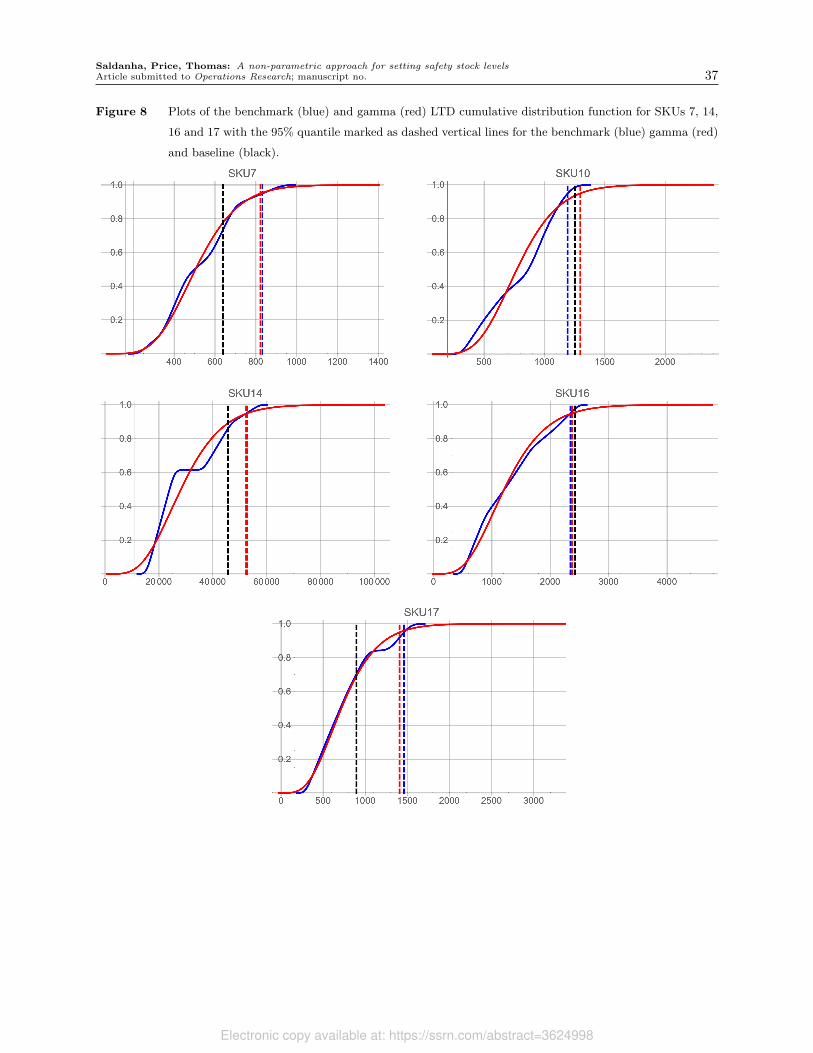
Saldanha, Price, Thomas: A non-parametric approach for setting safety stock levelsArticle submitted to Operations Research; manuscript no. 37
Figure 8 Plots of the benchmark (blue) and gamma (red) LTD cumulative distribution function for SKUs 7, 14,
16 and 17 with the 95% quantile marked as dashed vertical lines for the benchmark (blue) gamma (red)
and baseline (black).
Electronic copy available at: https://ssrn.com/abstract=3624998

e-companion to Saldanha, Price, Thomas: A non-parametric approach for setting safety stock levels ec1
Electronic Companion to “A non-parametric approach for
setting safety stock levels”
Appendix A: Intuition for Bootstrap Approach
To motivate our approach we relate our bootstrap algorithm to statistical sampling theory. We
assume LTD is an unobserved random variable X with an unknown distribution function FX with
the mean µX and the variance σ2X . Let us consider a theoretical framework where we can observe
realizations of the LTD random variable X, X = {x1, . . . , xnX}. We know in the development of
X, there are two random variables that represent lead time and demand and are independent. To
develop intuition for our proposal let us assume that lead time and demand are discrete random
variables and there exists n pairs, (li, di) ∈ Rli+1 such that xi =∑li
j=1 dij, ∀ii = 1, . . . , n. Note,
this assumes that lead time is paired with demand in the theoretical framework. Define L as the
vector of all li, and D as the vector of all di. Also assume we have observed samples of lead time
L= {l1, . . . , lnL} and demand D = {d1, . . . , dn
D}, which are not observed in pairs, and we assume
that the generating random variables of lead time and demand are independent. The bootstrap
method we propose is similar to developing a null distribution for a statistic of interest in bootstrap
hypothesis tests under the assumption that lead time and demand are independent. Furthermore, if
we assume that L and D, and D and L have the same empirical distributions, then the probability
of selecting a given sample of size nL, is exactly the same, which means the algorithm would
not recognize the two samples as different. This intuition leads to the idea that this bootstrap
methodology is attempting to create the sampling distribution of the statistic of interest, in this
case the safety stock, under the assumption that lead time and demand are independent.
Appendix B: Proof of Theorem 2
The proof of this theorem uses arguments from both Bickel and Freedman (1981), Ferguson (1998),
and Zou (2015)). We will provide a basic sketch of the proof as many of these results are well
known in the literature. Define x(1), . . . , x(n) to be the order statistics of the original sample and
x∗
(1), . . . , x∗
(n), be the order statistics of the bootstrap sample. Zou (2015) gives the the Bahadur
type representation of the bootstrap sample quantile as
Y ∗
p −Yp ≈Gn(F
−1X (p))−Fn(F
−1X (p))
fX(F−1X (p))
.
Using this representation we have that
√n(Y ∗
p −Yp
)≈
√n(Gn(F
−1X (p))−Fn(F
−1X (p))
)
fX(F−1X (p))
,
Electronic copy available at: https://ssrn.com/abstract=3624998

ec2 e-companion to Saldanha, Price, Thomas: A non-parametric approach for setting safety stock levels
where Fn is the empirical distribution function of the original sample and Gn is the empirical
distribution function of the bootstrap sample.
We use the approximation here because the other terms become negligible as n→∞ Based on
Theorem 4.1 in Bickel and Friedman (1981), we have that
√n(Gn(F
−1X (p))−Fn(F
−1X (p))
)
fX(F−1X (p))
=Wn(p)− pWn(1)
fX(F−1X (p))
→ W (p)− pW (1)
fX(F−1X (p))
.
Where W (p)− pW (1) is a Brownian Bridge. A similar result can be found in Zou (2015) and
Theorem 5.1 of Bickel and Freedman (1981). By using this result we can apply the same approach
as Ferguson (1998) to obtain the covariance of the bootstrap mean and bootstrap quantile.
To show the convergence of the mean, we again employ the Bahadur type representation of the
bootstrap sample quantile,
√n(x∗ − x) =
√n
n
n∑
i=1
(x∗
i −xi)
=
√n
n
n∑
i=1
(x∗
(i) −x(i))
=
√n
n
n∑
i=1
(G−1
n (i
n+1)−F−1
n (i
n+1)
)
=1
n
n∑
i=1
Wn(i
n+1)− i
n+1Wn(1)
f(F−1( i
n+1))
→∫ 1
0
W (t)− tW (t)
f(t)dt
From here we can show that the two quantiles are asymptotically bivariate normal using the
Cramer-Wold device. The variances of each quantity are known from Bickel and Friedman (1981),
all that is left is to find the covariance. Based on the asymptotic results, we must find
Cov
(W (p)− pW (1)
f(F−1(p)),
∫ 1
0
(W (t)− tW (t))dt
f(t)
).
This proof is given in Ferguson (1998), and the theorem is complete.
Appendix C: Bootstrap Tuning Parameters
Here we develop guidance on the bootstrap tuning parameters, i.e., the bootstrap sample size (m)
and number of bootstrap samples (B). We use the identical lead time and demand distribution
inputs from Table 1 & Table 2 of the article. In Table EC.1 we provide the experimental levels of
the bootstrap parameters and empirical data inputs. We varied the number of bootstrap re-samples
Electronic copy available at: https://ssrn.com/abstract=3624998

e-companion to Saldanha, Price, Thomas: A non-parametric approach for setting safety stock levels ec3
B, the sample size of the empirical data for lead time (nL) and demand (nD) and the bootstrap
sample sizem. Supply chain managers have less control of nL and nD that depend upon the demand
and replenishment processes that are governed by many other factors such as the inventory control
policy, order sizes and, purchasing and production economies of scale. The bootstrap sample size
is known to be statistically important for the asymptotic convergence of the bootstrap estimator
Bickel and Freedman (1981). Bootstrap theory prescribes that the bootstrap sample size should be
at most the sample size of the observed data Efron and Tibshirani (1986). This is a critical result
for bootstrapping the LTD distribution from empirical lead-time and empirical demand data due
to the fact that LTD data are not directly observed, which is a common occurrence (Das et al.
2014, Rossetti and Unlu 2011). Hence, the sample size of the LTD data, nx, is typically unknown
and thus the sample size m of each bootstrap resample b∈B cannot be determined.
Table EC.1 Experimental levels for exploring the bootstrap tuning parameters of bootstrap resampling
replications (B) and bootstrap sample size (m) for setting the ROP with different levels of empirical lead time (nL)
and demand (nD) sample sizes, respectively.
Parameter Experimental Levels
Lead Time Sample Size (nL) 6, 10, 24, 50, 100Demand Sample Size (nD) 0.5nL, nL, 1.5nL
Bootstrap Sample Size (m) nL, 2nL, 3nL
Bootstrap Replications (B) 500, 1000
On the one hand, the intuition that LTD is the sum of demands conditioned on lead times; hence,
the number of LTD data is equivalent to the number of lead time data dictates that m= nL. On
the other hand, it could be argued that in the compound distribution setting sample lead times
and sample demands are assumed to be independent draws from independent random variables
then m could be the sample size of all possible random sum mixtures of the sample lead times and
sample demands. This would require us to setm>nL and the use of sub-sampling strategies (Bickel
et al. 1997, Gotze 1993). To determine the appropriate m we conduct simulation experiments
where m≥ nL, which also shed light on the bias and inconsistency of bootstrap estimates from not
employing the appropriate values of the bootstrap sample size, m. In the experiments we estimate
the bootstrap quantile but these results are easily extended to that of the bootstrap safety stock
estimator.
We conduct 100 replications of all levels of the experimental factors in Table EC.1 for quan-
tiles corresponding to P1 = 60%–99% in 5% increments, for each of the 8 lead-time distributions
from Table 1 and Table 2 of the article; a total of 6,480 experiments. For each replication of
each experimental cell we drew a random sample L= {l1, . . . , lnL} and demand D = {d1, . . . , dn
D}
Electronic copy available at: https://ssrn.com/abstract=3624998

ec4 e-companion to Saldanha, Price, Thomas: A non-parametric approach for setting safety stock levels
from the parent lead time and demand distributions, respectively. The bootstrap algorithm is
used to bootstrap an m size empirical distribution of the b-th bootstrap LTD mixture X(b) =
{x(b)1 , . . . , x(b)
nm} with replacement from L and D for B bootstrap replications. For each replication
r = 1, . . . ,100 we estimate Y ∗
P1,r=
∑B
b=1 Y(b)P1,r
/B with the corresponding standard error sY ∗
P1,r=
√B−1
∑B
b=1
(Y
(b)P1,r
− Y ∗
P1,r
)2
where Y(b)P1,r
is the bootstrap estimate for the P1-th quantile of the
b-th bootstrap resample and the r-th experimental replication. We then calculate the number of
standard errors the bootstrap quantile is from the true quantile YP1for each replication using the
z-score calculated as zr =Y ∗
P1,r−YP1
sY ∗
P1,r
. This approach allows us to evaluate how well the bootstrap
performs in encompassing the true quantile YP1, in a confidence interval. Hence, the bootstrap
mean and standard deviation of the quantile statistics offers useful insights on the variability of the
estimate. The z-score conveys the variability of the estimate from the truth. These values under-
score the robustness of the bootstrap method by clearly specifying how many times the bootstrap
quantile Y ∗
P1is a certain number of standard errors away from YP1
the true quantile.
We calculate true quantile YP1using Monte-Carlo procedures fixing the random seed with 1
million random draws from the parent lead time distribution and for each lead time li the corre-
sponding lead time demand x1 =∑li
j=1 dj. The z-scores from the previous step are then arranged
in ascending order and the 95-th z-score indicates that the bootstrap quantile Y ∗
P1,ris within sY ∗
P1,r
standard errors of the true YP195% of the time. The goal is to approximate large sample theory
where all 95% quantiles are close to 2 standard errors from the true ROP. This procedure also
follows current practice where the reporting of test statistics is becoming more prevalent so exper-
iments are reproducible and transparent, as advocated by the American Statistical Association
Wasserman and Lazar (2016).
C.1. Tuning Experiment Results
The experiments are run in R version 3.5.2 on a Unix system in a high performance computing
cluster with fixed random seeds to ensure results are reproducible. In Table EC.2 the colored heat
map represents the z-score values ranging from the lowest (most desirable) values in green and
highest (least desirable) values in red, with intermediate ranges graded accordingly with yellow.
The z-scores are calculated for the bootstrap sample quantile estimate using 1,000 resamples for
lognormal lead time (µL = 5 and CVL = 0.4) across a selection of values of m, nL, nD and PNS. We
see the lowest z-scores when m= nL and, for higher nL and nD. From our experiments we notice
that the z-scores appear to get higher (indicating more bias) with greater right skew (higher CV)
at higher PNS (results available from the authors). This is because at extreme right skew, fewer
LTD samples in each bootstrap are drawn from the extremities of the right tail, which cautions
Electronic copy available at: https://ssrn.com/abstract=3624998

e-companion to Saldanha, Price, Thomas: A non-parametric approach for setting safety stock levels ec5
Table EC.2 Bootstrap of the quantile with an (s, Q) policy for 100 replications of the LTD mixture bootstrap
1,000 times from lognormal distributed lead time (µL = 5 and CVL = 0.4), and gamma distributed demand (µD =
100 and CVD = 0.2) across different levels of PNS and, sample sizes for the mixtures of lead-time demand (m), lead
time (nL) and demand (nD).
PNSm/nL nL nD/nL 60% 65% 70% 75% 80% 85% 90% 95% 99%
1
6
0.5 2.799 3.034 3.238 3.781 4.457 5.997 8.038 10.321 17.8001 2.015 2.571 2.774 3.170 3.895 5.314 7.119 10.187 17.453
1.5 1.725 1.996 2.574 3.140 3.529 4.817 6.470 9.411 15.340
24
0.5 2.627 2.631 2.661 2.998 3.045 3.307 3.153 4.013 8.3421 2.242 2.405 2.611 2.892 3.083 3.228 3.259 4.352 8.449
1.5 2.435 2.475 2.389 2.909 2.776 2.919 2.790 3.831 7.990
100
0.5 2.440 2.414 2.366 2.351 2.242 1.903 2.014 2.107 4.9571 1.903 1.939 2.013 1.937 2.072 1.875 1.950 2.323 4.931
1.5 1.774 1.939 1.930 2.031 1.940 1.705 1.950 2.277 4.803
2
6
0.5 4.160 3.899 4.274 5.135 6.251 7.938 9.510 13.765 25.0371 3.065 3.124 3.522 4.354 5.633 7.481 9.353 14.205 22.819
1.5 2.601 2.654 3.298 3.871 4.956 6.498 8.134 12.745 21.915
24
0.5 3.622 3.651 3.684 3.936 4.318 4.539 4.135 5.044 11.0851 3.208 3.515 3.613 4.078 4.337 4.132 4.125 5.298 10.912
1.5 3.271 3.589 3.763 4.309 4.164 4.280 3.652 4.719 10.078
100
0.5 3.399 3.473 3.300 3.247 3.085 2.818 2.915 2.720 5.9741 2.803 2.685 2.775 2.680 2.805 2.703 2.557 3.027 5.964
1.5 2.587 2.693 2.704 2.720 2.856 2.407 2.665 3.078 6.170
3
6
0.5 5.017 5.097 4.753 5.529 7.076 8.987 11.333 16.889 29.8671 3.617 3.680 4.203 5.350 7.045 9.088 11.746 16.809 27.920
1.5 3.189 3.161 3.784 4.534 6.002 7.531 10.312 14.481 26.068
24
0.5 4.482 4.425 4.377 4.681 5.274 5.708 4.873 6.004 13.1081 4.010 4.455 4.758 5.090 5.336 5.101 4.928 6.077 13.078
1.5 3.840 4.389 4.717 4.980 5.194 5.227 4.569 5.211 12.276
100
0.5 4.293 4.212 4.071 4.134 3.817 3.458 3.509 3.305 6.9061 3.417 3.520 3.328 3.230 3.478 3.289 3.117 3.624 7.027
1.5 3.141 3.158 3.172 3.401 3.573 2.978 3.332 3.619 7.308
use of the bootstrap in the presence of outliers. Nevertheless, even for this high skew when m= nL
the z-score is significantly lowered and close to three standard errors away from the true.
These results are consistent for all distributions (additional results are available from the
authors). The primary takeaway from these results is that using a bootstrap sample size of m= nL
will give estimates and standard errors that can be trusted for decision-making purposes. This
result conforms to the intuition that the number of lead time demands observed should correspond
to the number of lead times observed.
Electronic copy available at: https://ssrn.com/abstract=3624998

ec6 e-companion to Saldanha, Price, Thomas: A non-parametric approach for setting safety stock levels
Appendix D: Industry Simulation Validation
The inputs and lead-time and demand statistics for each of the 9 SKUs used in the simulation
are presented in Table EC.3. We use the MakerCo lead-time and demand data to construct the
benchmark LTD distributions.
Table EC.3 Industry simulation inputs
SKU Order Avg. Std. Dev. Avg. Std. Dev Baseline BaselineQuantity (Q)* Lead Time† Lead Time† Demand† Demand† Safety Stock* Reorder Point
3 350 78.1 46.4 14.8 5.7 2,100 3,2586 3,380 119.9 27.4 34.5 7.1 2,540 6,6787 219 105.5 35.6 5 1.5 110 6389 441 149.5 40.4 2.4 1.7 440 792
10 1,760 115.8 41.1 7 4.7 440 1,25213 2,310 160.5 78.2 63.5 31.5 2,310 12,50414 20,600 204.7 104.9 147.3 30.2 15,450 45,60616 709 116.1 57.7 11.2 1.6 1,120 2,42117 238 91.2 50.6 7.8 4.6 180 894
Note:*Taken directly from inventory sheet data†Calculated from the order lead time and demand data
The LTD distributions for each of the 9 SKU’s are provided in Figure EC.1. These are the
benchmark distributions that we considered the “true” distributions for computing the reorder
point, safety stocks, µX , σX and other LTD statistics. We use these for both establishing the
internal and external validity of our simulation and, the benchmarks for comparing the bootstrap,
baseline and gamma estimates.
Electronic copy available at: https://ssrn.com/abstract=3624998

e-companion to Saldanha, Price, Thomas: A non-parametric approach for setting safety stock levels ec7
FigureEC.1
Ben
chmark
leadtimedem
anddistributionsforthe9SKUs.
Electronic copy available at: https://ssrn.com/abstract=3624998

ec8 e-companion to Saldanha, Price, Thomas: A non-parametric approach for setting safety stock levels
For establishing internal validity of the simulation model we constructed 95% confidence intervals
for the mean deviation (MD) of the simulation LTD statistics from the true LTD statistics. We ran
10 replication of the simulation for each of the three models (bootstrap, baseline and bootstrap)
and each of the 9 SKUs with each replication simulating 25 years with a 25 year warm-up. We
report 95% confidence intervals for LTD statistics of the baseline simulation in Table EC.4.
Table EC.4 95% Upper confidence level (UCL) and lower confidence level (LCL) of the mean difference (∆) in
the true and simulated µX and σX for the baseline simulation across all SKUs
µX σX
SKU Benchmark Mean ∆ S.D. ∆ UCL LCL Benchmark Mean ∆ S.D. ∆ UCL LCL
3 1,166.8 10.4 36.0 36.2 -15.4 653.4 -0.4 21.9 15.3 -16.06 4,234.5 -13.0 81.9 45.6 -71.6 931.0 -8.8 35.0 16.2 -33.87 517.4 -1.9 12.6 7.1 -10.9 166.7 -4.2 6.7 0.5 -9.09 377.3 4.3 13.1 13.7 -5.1 95.6 2.1 4.5 5.3 -1.1
10 857.8 7.5 68.9 56.7 -41.8 304.7 -8.1 37.9 19.0 -35.213 10,405.2 79.1 249.6 257.6 -99.5 4,668.6 -5.8 148.9 100.7 -112.414 30,955.9 83.0 1,454.9 1,123.8 -957.8 12,772.2 -172.3 828.3 420.3 -764.816 1,284.7 -37.6 51.0 -1.2 -74.1 573.5 -4.7 28.9 16.0 -25.317 755.8 3.3 10.4 10.7 -4.2 343.9 -3.3 12.4 5.6 -12.1
To establish external validity of our simulation we generated graphical output from all 9 SKUs
that we shared with the managers of MakerCo to. We present SKU 3 in Panel A and SKU 17 in
Panel B as exemplars in Figure EC.2. With managers feedback we were able to validate that our
simulation was closely approximating their replenishment and inventory processes.
Electronic copy available at: https://ssrn.com/abstract=3624998