A Non-Linear Stochastic Model for Inflation

Robert S. Clarkson

The Scottish Mutual Assurance Society, 109 St. Vincent Street, Glasgow G2 5HN, United Kingdom

Summary

The paper describes the construction of a non-linear stochastic model for inflation where the expected value of the residual varies with the recent level of inflation. It is shown that this model gives a better representation of the post-war UK inflation experience than the IRIMA inflation model that forms part of the comprehensive stochastic investment model constructed by Wilkie (1986). Three general criteria of suitability of a stochastic model are deduced from the construction and testing of the non-linear mode. It is also shown that the general formulation of the model may have applications in other areas such as stockmarket volatility where the system displays periods of very high variability that cannot be represented satisfactorily in terms of a linear model.

Résumé

Un Modèle Stochastique Non Linéaire pour l'Inflation

L’article décrit la construction d’un modèle stochastique non-linéaire pour l’inflation dans lequel la valeur attendue de la valeur résiduelle varie avec le récent niveau d’inflation. On y montre que ce modèle donne une meilleure représentation de l’inflation britannique d’après- guerre que le modèle d’inflation ARIMA qui fait partie du modèle d’investissement stochastique complet construit par Wilkie (1986). Trois critères généraux d’aptitude d’un modèle stochastique sont déduits de la construction et des tests du modèle non-linéaire. L’article montre également que la formulation générale du modèle peut avoir des applications dans d’autres domaines tels que la volatilité de la bourse des valeurs où le système présente des périodes de très haute variabilité qui ne peuvent pas être représentées de façon satisfaisante avec un modèle linéaire.

233

1. Introduction

The role of the actuary has recently been defined very aptly and very succinctly as offering expert and relevant solutions to uncertain future events. In areas such as life insurance, the principles underlying these “expert and relevant” solutions are so well established that they are rarely debated by the profession; the sciences of compound interest and life contingencies provide the computational framework for dealing with future investment returns and future mortality, and once the actuary has selected a suitable basis for interest rates, mortality and any other relevant variables, there are well-defined techniques for calculating whatever derived information is required.

In the area of financial risk, the scientific methods are currently at a much earlier stage of development. Actuaries in many countries are not only looking for practical solutions to certain problems but are also developing theoretical methods that may be of more generalapplication. All this work is certainly “expert”, but it may be many years before there is general agreement as to what methods are “relevant” in particular application areas.

The underlying theme of this paper is that certain of the simplifying assumptions behind many financial models, e.g. that distributions are normal (or gaussian) or that the system is linear, may not be satisfactory in certain application areas, with the result that conventional statistical tests may be inappropriate when assessing the suitability of a particular model.

The major part of this paper describes a non-linear stochastic model for inflation, with the general structure of the model being built up from a consideration of the mechanisms that need to be included to replicate the observed general properties of UK inflation in recent decades. Once this model has been constructed and compared with a linear model based on the autoregressive integrated moving average (ARIMA) approach, generalisations are drawn as to what suitability criteria are appropriate. The final part of the paper extends the discussion to other areas such as option pricing and studies of stockmarket efficiency.

234

2. Construction of the model

On the basis that there are three main mechanisms which affect the year-on-year inflation rate i t :

i) a tendency for the rate to return to some “intrinsic” value,

ii) a random error component which operates every year,

and iii) a random shock component which operates infrequently,

I believe that an appropriate general model is:

where A t > 0

B is the “intrinsic” rate

D t is the random error term

and E t is the random shock term.

Some very general properties of these auxiliary functions A of inflation. Inflation is essentially a symptom of t , D t and E t can be deduced from certain characteristics

instability in an economic system. Because of various linkages with wages and prices, negative inflation rates are uncommon, but instability as a result of domestic circumstances (e.g. lax monetary policy) or external effects (e.g. the first and second “oil shocks”) can result in a marked rise in the inflation rate above the intrinsic rate. When the rate of inflation is low and has been relatively stable for a number of years, the year-on-year variability is significantly lower than when recent rates have been high.

A constant value for A t would imply a constant rate of return to the intrinsic rate. To provide a mechanism for the rate of inflation rising well above the intrinsic rate as a result of domestic conditions it is desirable to use a lower value of A t when there is an upward trend in inflation. This can be achieved by replacing the term

235

by

where A and C are positive constants and Trend {i the recent trend rate of change of inflation when this is

t-1 } is +

positive and zero otherwise.

To allow for the higher variability of inflation when recent rates have been high, the random error term can be expressed as D(t-1).Z(t) where D(t-1) is positive and increases with the recent geometric average rate of inflation and Z(t) is a random unit normal variate.

Since the centralising and random error terms provide the mechanism for a large negative impulse when inflation is high but cannot provide the mechanism for a large positive impulse when inflation is low, the random shock term can be regarded as "upward only" and defined as p(t)E(t) where p(t) is the probability that the random shock operates at time t and E(t) is the value of the shock if it occurs at time t.

This model for inflation, namely

contains one linear and three non-linear components.Because of feedback from one non-linear component to another, the patterns of inflation that can be generated by this apparently simple formulation are many and varied. In particular, the model can operate for a period in what may be called its "quiescent phase", with relatively low and stable rates of inflation. Then any one of the non-linear components can trigger an "active phase" in which inflation rates are higher and more variable. The linear centralising component provides the mechanism which in due course takes the model back to another quiescent phase.

Since this type of non-linear model is much closer to a "Chaos Theory" artifact than to a linear situation which can be analysed by standard statistical techniques, there are no "textbook" methods of assessing whether my model is "satisfactory" or of estimating the numerous parameters involved. However, if there is a linear inflation model which has been fitted and tested by conventionalstatistical techniques, we can use it as a benchmark for assessing my non-linear model by asking the question:

236

"What deductions can we make about the use of the linear model as a description of the post-war UK inflation experience if all three non-linear mechanisms operated over this period?"

3. Comparison with the Wilkie inflation model

Wilkie (1986) has constructed a stochastic investment model for actuarial use which can be used for simulations of "possible futures" extending for many years ahead. The model consists of a set of interrelated autoregressive equations which generate at yearly intervals the rate of inflation, the gilts yield, the ordinary share yield, and ordinary share dividends. In particular, the inflation model suggested by Wilkie is:

where Z(t) is a random unit normal variate.

Since log(1+x) is approximately equal to x when x is small,the Wilkie inflation model can be rewritten as:

This is a very special case of my model with all three non- linear elements suppressed; in the case of the "trend" and "shock" elements, C and E(t) are zero, and in the case of the random error D(t-l) is replaced by a constant. We can therefore take the Wilkie model as the "best" available linear model and use it as the benchmark against which to assess my non-linear model.

Of the three non-linear components, the random shock operates only occasionally, the upward trend element comes into play only part of the time, but the random error operates every year. Accordingly, the non-linear random error term should be the easiest to identify. In fitting any linear model, it is assumed that the expected value of the random error is constant. If this proves not to be the case, then any linear model will probably be inappropriate.

It is desirable to have some "absolute" test of whether the linear model can generate inflation scenarios similar to the post-war experience. Since this model is of the form:

237

t where it is the force of inflation, A, B and C areconstants and Z(t) is a random unit normal variate, using the model to simulate inflation scenarios essentially involves :

i) using random numbers to specify percentile points in the distribution function of the normal variate,

ii) calculating the value of Z(t) at this percentile point,

and iii) calculating the next inflation value using the above formula.

Given any actual inflation scenario, this process can be run in reverse. gives Z(t),

Substituting the values of i t and i and from Z(t) the percentile point can be

t-1

calculated. The values so derived (which can be assumed for simplicity to be integers in the range 1, 2, ... 98, 99, 100) should be random in both order and frequency if the model is consistent with the actual scenario. This provides a very convenient nul hypothesis by which to judge the linear model, namely that the percentile values generated by running the model against the post-war experience are random in both order and frequency.

Since the linear model has no separate "shock" component, both the normal variability and the occasional very large positive residual have to be accommodated by the (uniform) residual variance. This means that between periods of high inflation the linear model will overstate the year-on-year variability. During periods of low or moderate inflation, the average size of the residual Z(t) will therefore be significantly lower than predicted by the linear model. Accordingly, there will be long runs of residuals less than, say, one standard deviation in absolute magnitude and the percentile values - in terms of order - will thus be inconsistent with the nul hypothesis of randomness.

Furthermore, if the residuals do indeed vary in expected value with the level of inflation, then during periods of low inflation the residuals will be very low compared to the values expected using the linear model. These two factors combined would give far more than the expected 50% of percentile points in the range 26 to 75, with a distinct peak in the very centre, say in the range 46 to 55.

238

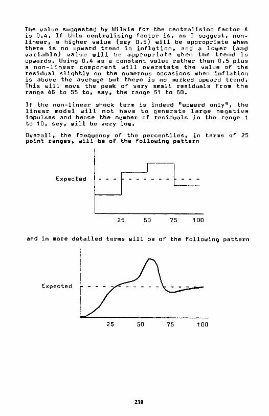
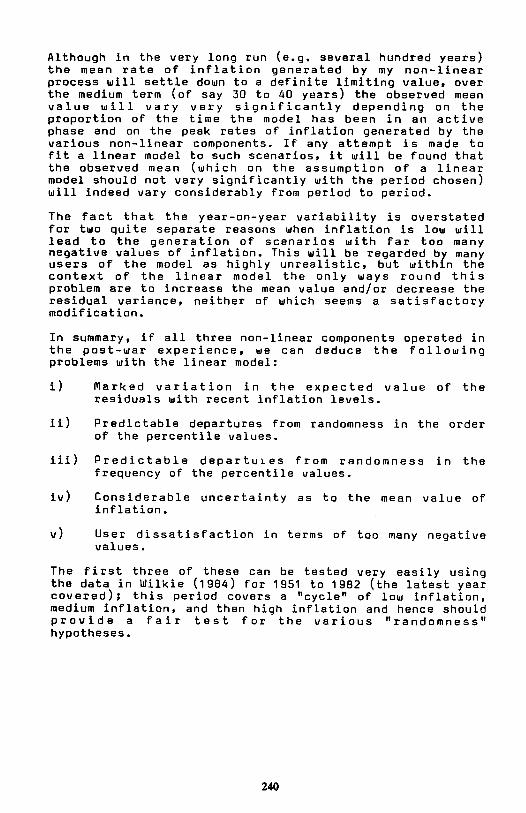
The value suggested by Wilkie for the centralising factor A is 0.4. I f this centralising factor is, as I suggest, non- linear, a higher value (say 0.5) will be appropriate when there is no upward trend in inflation, and a lower (and variable) value will be appropriate when the trend is upwards. Using 0.4 as a constant value rather than 0.5 plus a non-linear component will overstate the value of the residual slightly on the numerous occasions when inflation is above the average but there is no marked upward trend. This will move the peak of very small residuals from the range 46 to 55 to, say, the range 51 to 60.

If the non-linear shock term is indeed “upward only”, the linear model will not have to generate large negative impulses and hence the number of residuals in the range 1 to 10, say, will be very low.

Overall, the frequency of the percentiles, in terms of 25 point ranges, will be of the following pattern

Expected

25 50 75 100

and in more detailed terms will be of the following pattern

Expected

25 50 75 100

239

Although in the very long run (e.g. several hundred years) the mean rate of inflation generated by my non-linear process will settle down to a definite limiting value, over the medium term (of say 30 to 40 years) the observed mean value will vary very significantly depending on the proportion of the time the model has been in an active phase and on the peak rates of inflation generated by the various non-linear components. If any attempt is made to fit a linear model to such scenarios, it will be found that the observed mean (which on the assumption of a linear model should not vary significantly with the period chosen) will indeed vary considerably from period to period.

The fact that the year-on-year variability is overstated for two quite separate reasons when inflation is low will lead to the generation of scenarios with far too many negative values of inflation. This will be regarded by many users of the model as highly unrealistic, but within the context of the linear model the only ways round this problem are to increase the mean value and/or decrease the residual variance, neither of which seems a satisfactory modification.

In summary, if all three non-linear components operated in the post-war experience, we can deduce the following problems with the linear model:

i) Marked variation in the expected value of the residuals with recent inflation levels.

ii) Predictable departures from randomness in the order of the percentile values.

iii) Predictable departures from randomness in the frequency of the percentile values.

iv) Considerable uncertainty as to the mean value of inflation.

v) User dissatisfaction in terms of too many negative values.

The first three of these can be tested very easily using the data in Wilkie (1984) for 1951 to 1982 (the latest year covered); this period covers a "cycle" of low inflation,medium inflation, and then high inflation and hence should provide a fair test for the various "randomness" hypotheses.

240

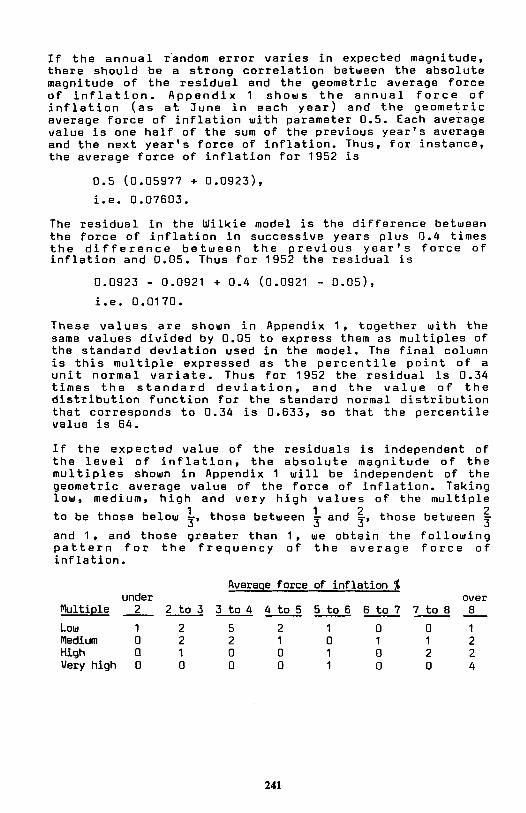
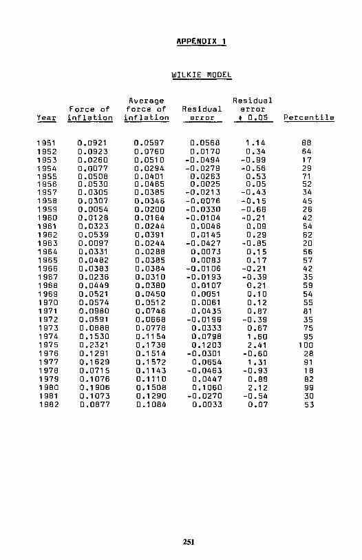
If the annual random error varies in expected magnitude, there should be a strong correlation between the absolute magnitude of the residual and the geometric average force of inflation. Appendix 1 shows the annual force of inflation (as at June in each year) and the geometric average force of inflation with parameter 0.5. Each average value is one half of the sum of the previous year’s average and the next year’s force of inflation. Thus, for instance, the average force of inflation for 1952 is

0.5 (0.05977 + 0.0923),

i.e. 0.07603.

The residual in the Wilkie model is the difference between the force of inflation in successive years plus 0.4 times the difference between the previous year’s force of inflation and 0.05. Thus for 1952 the residual is

0.0923 - 0.0921 + 0.4 (0.0921 - 0.05),

i.e. 0.0170.

These values are shown in Appendix 1, together with the same values divided by 0.05 to express them as multiples of the standard deviation used in the model. The final column is this multiple expressed as the percentile point of a unit normal variate. Thus for 1952 the residual is 0.34 times the standard deviation, and the value of the distribution function for the standard normal distribution that corresponds to 0.34 is 0.633, so that the percentile value is 64.

If the expected value of the residuals is independent of the level of inflation, the absolute magnitude of the multiples shown in Appendix 1 will be independent of the geometric average value of the force of inflation. Taking low, medium, high and very high values of the multiple

and 1, and those greater than 1, we obtain the following pattern for the frequency of the average force of inflation.

Average force of inflation %under over

Multiple 2 2 to 3 3 to 4 4 to 5 5 to 6 6 to 7 7 to 8 8

Low 1 2 5 2 1 0 0 1 Medium 0 2 2 1 0 1 1 2 High 0 1 0 0 1 0 2 2 Very high 0 0 0 0 1 0 0 4

241

to be those below 1 3 , those between 1 3

and 2 3 , those between 2

3

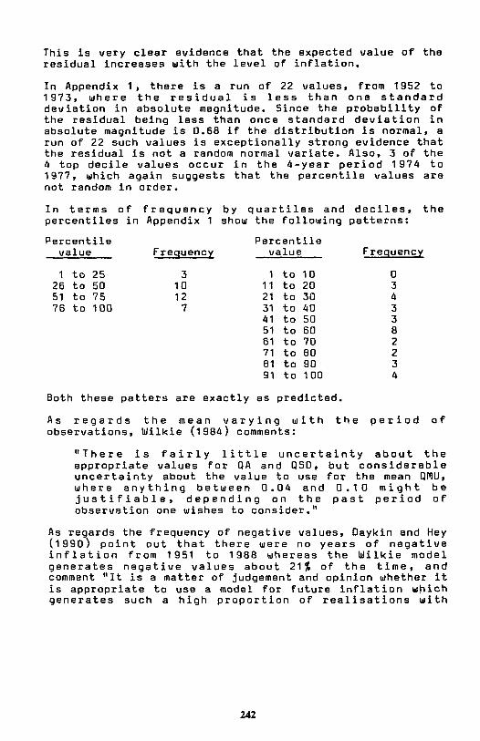
This is very clear evidence that the expected value of the residual increases with the level of inflation.

In Appendix 1, there is a run of 22 values, from 1952 to 1973, where the residual is less than one standard deviation in absolute magnitude. Since the probability of the residual being less than once standard deviation in absolute magnitude is 0.68 if the distribution is normal, a run of 22 such values is exceptionally strong evidence that the residual is not a random normal variate. Also, 3 of the 4 top decile values occur in the 4-year period 1974 to 1977, which again suggests that the percentile values are not random in order.

In terms of frequency by quartiles and deciles, the percentiles in Appendix 1 show the following patterns:

percentile value Frequency

Percentile value Frequency

1 to 25. 3 1 to 10 26 to 50 10 11 to 20 51 to 75 12 21 to 30 76 to 100 7 31 to 40

41 to 50 51 to 60 61 to 70 71 to 80 81 to 90 91 to 100

0 3 4 3 3 8 2 2 3 4

Both these patters are exactly as predicted.

As regards the mean varying with the period of observations, Wilkie (1984) comments:

"There is fairly little uncertainty about the appropriate values for QA and QSD, but considerable uncertainty about the value to use for the mean QMU, where anything between 0.04 and 0.10 might be justifiable, depending on the past period of observation one wishes to consider."

As regards the frequency of negative values, Daykin and Hey (1990) point out that there were no years of negative inflation from 1951 to 1988 whereas the Wilkie model generates negative values about 21% of the time, and comment "It is a matter of judgement and opinion whether it is appropriate to use a model for future inflation which generates such a high proportion of realisations with

242

negative inflation. This can be mitigated by increasing the mean value of the inflation model and by reducing the standard deviation of the random element."

Since all five of the predicted behavioural aspects have been clearly identified, a non-linear model of the type I have outlined is likely to give a far better representation of the post-war UK inflation experience than any linear model. Also, because of the explicit formulation of my model, it is possible to arrive at satisfactory auxiliary functions and plausible values for the various parameters without having to carry out any elaborate estimation procedures.

As discussed earlier, for the centralising factor A the value should be somewhat higher than the value of 0.4 that is suitable in the case of the linear model, and so a value of 0.5 seems reasonable.

For the intrinsic force of inflation, which essentially is a "normal" minimum level, a value of 0.04 seems reasonable; this corresponds to an annual rate of inflation slightly greater than 4%.

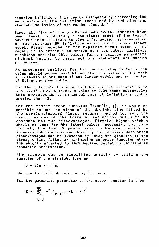
For the recent trend function Trend + (i t-1 ), it would be possible to use the slope of the straight line fitted by the straightforward "least squares" method to, say, the last 5 values of the force of inflation, but such an approach has two disadvantages. Firstly, higher weights should be used for the latest values; secondly, the data for all the last 5 years have to be used, which is inconvenient from a computational point of view. Both these disadvantages can be overcome by using the gradient of the straight line fitted by minimising an error function where the weights attached to each squared deviation decrease in geometric progression.

The algebra can be simplified greatly by writing the equation of the straight line as:

Y = a(x-n) + b,

where n is the last value of x, the year.

For the geometric parameter r, the error function is then

243

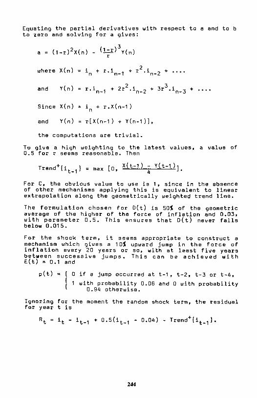
Equating the partial derivatives with respect to a and to b to zero and solving for a gives:

the computations are trivial.

To give a high weighting to the latest values, a value of 0.5 for r seems reasonable. Then

For C, the obvious value to use is 1, since in the absence of other mechanisms applying this is equivalent to linear extrapolation along the geometrically weighted trend line.

The formulation chosen for D(t) is 50% of the geometric average of the higher of the force of inflation and 0.03, with parameter 0.5. This ensures that D(t) never falls below 0.015.

For the shock term, it seems appropriate to construct a mechanism which gives a 10% upward jump in the force of inflation every 20 years or so, with at least five years between successive jumps. This can be achieved with E(t) = 0.1 and

p(t) = { 0 if a jump occurred at t-l, t-2, t-3 or t-4,

1 with probability 0.06 and O with probability0.94 otherwise.

Ignoring for the moment the random shock term, the residual for year t is

244

{

{

and

and

where

Since

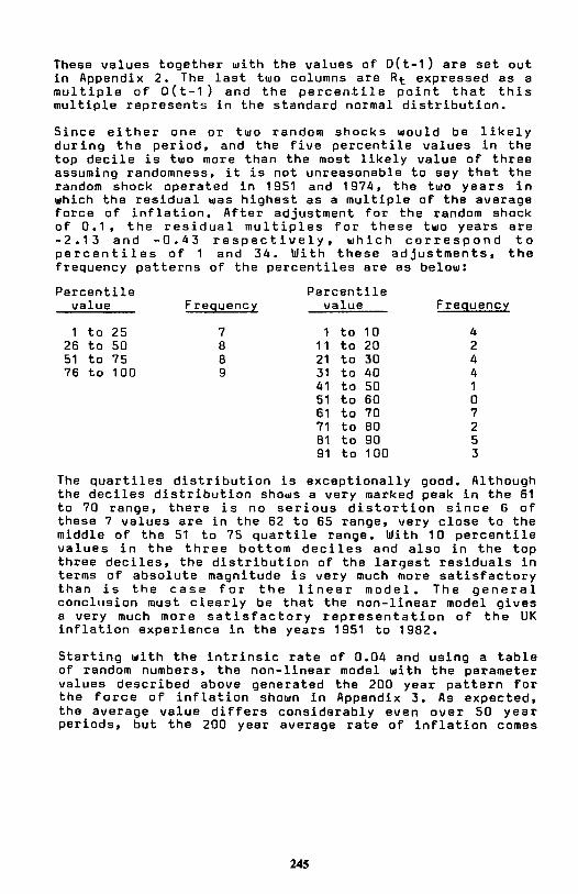
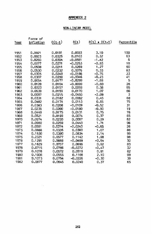
These values together with the values of D(t-1) are set out in Appendix 2. The last two columns are R t expressed as a multiple of D(t-1) and the percentile point that this multiple represents in the standard normal distribution.

Since either one or two random shocks would be likely during the period, and the five percentile values in the top decile is two more than the most likely value of three assuming randomness, it is not unreasonable to say that the random shock operated in 1951 and 1974, the two years in which the residual was highest as a multiple of the average force of inflation. After adjustment for the random shock of 0.1, the residual multiples for these two years are -2.13 and -0.43 respectively, which correspond to percentiles of 1 and 34. With these adjustments, the frequency patterns of the percentiles are as below:

Percentile value Frequency

Percentile value Frequency

1 to 25 7 1 to 10 26 to 50 8 11 to 20 51 to 75 8 21 to 30 76 to 100 9 31 to 40

41 to 50 51 to 60 61 to 70 71 to 80 61 to 90 91 to 100

4 2 4 4 1 0 7 2 5 3

The quartiles distribution is exceptionally good. Although the deciles distribution shows a very marked peak in the 61 to 70 range, there is no serious distortion since 6 of these 7 values are in the 62 to 65 range, very close to the middle of the 51 to 75 quartile range. With 10 percentile values in the three bottom deciles and also in the top three deciles, the distribution of the largest residuals in terms of absolute magnitude is very much more satisfactory than is the case for the linear model. The general conclusion must clearly be that the non-linear model gives a very much more satisfactory representation of the UK inflation experience in the years 1951 to 1982.

Starting with the intrinsic rate of 0.04 and using a table of random numbers, the non-linear model with the parameter values described above generated the 200 year pattern for the force of inflation shown in Appendix 3. As expected, the average value differs considerably even over 50 year periods, but the 200 year average rate of inflation comes

245

out at 6.00%, which suggests that the parameter values are realistic. Also, there were only 7 negative values of the force of inflation, the largest in absolute magnitude being 3.04%.

The very comprehensive estimation procedures andstatistical tests in Wilkie (1984) identify the most suitable ARIMA model for UK inflation but cannot provide a complete answer to the question "Is an ARIMA model appropriate?" It is clearly impossible to assess mynon-linear model on the basis of conventional statistical tests. Instead, I believe that any stochastic model, whether linear or non-linear, should be assessed both for general suitability and also for the appropriateness of the specific parameter values on the basis of the following criteria:

1. The mechanisms implied by the model should be plausible on economic grounds.

2. The parameter values and auxiliary functions should be such that, in fitting the model to the past experience, the standardised residuals (e.g. the residuals divided by D(t-1) in the case of my non-linear model) should be consistent with a random unit normal variate not only in terms of frequency but also in terms of order.

3. The parameter values and auxiliary functions should be plausible on economic grounds.

The second criterion is of course quite different from and much stronger than most conventional statistical tests, which generally assume that the residuals are normal in frequency and ignore the question of order. The other two reflect the importance of the model being seen by users as a plausible representation of real-world phenomena. If a model meets all three of these criteria, then within its application domain it is highly likely that it will provide solutions that are not only "expert" but also "relevant".

An increasing awareness by statisticians in recent years of the limitations of linear models as representations of many economic and financial series has led Engle (1982) and others to develop autoregressive conditionalheteroscedastic (ARCH) models to remove the implausible assumption of a constant variance. However, as with ARIMA models, the statistical tests only address the question of whether a particular model is the best of its class rather than addressing the more fundamental question of whether any model of that class offers a satisfactory

246

representation. Also, asymmetric non-linear components such as the upward-only trend component in my non-linear model cannot be incorporated.

4. Option pricing models

Brancovan, Dehapiot and Zamfirescu (1989) show how the constant volatility assumption of the Black-Scholes option pricing model can be relaxed to allow volatility to be a two-state stochastic process and comment that this approach can be extended by using simulations involving a more complicated stochastic model for volatility.

Walter (1989) also refers to the problem of volatility instability and develops the ideas of Mandelbrot (1963) and others by describing how Levy-stable distributions can provide much more realistic descriptions of certain economic and financial variables than can be obtained using the normal distribution.

In many ways equity price volatility, both at the individual stock level relative to the market and at the market level, is similar to inflation. There is some minimum level below which it rarely falls, but sometimes periods of higher volatility occur and occasionally (as for instance in October 1987) exceptionally high volatility arises. After a period of high volatility, the level tends to decrease back towards a more normal level.

This behaviour can be represented very satisfactorily using exactly the same form of stochastic model as the non- linear inflation model discussed above except that the random error is constrained to be positive to avoid negative values arising.

It can easily be shown that the first differences of values generated by my non-linear model have the "fatter tails" property described by Mandelbrot (1963) and others. For example, this is the case for the 200 inflation values fitted in Appendix 3. A smoother progression could be obtained by extending the simulations for several thousand years, but even in separate subgroups of fifty years the general pattern is clearly visible.

Although Levy distributions can offer a betterrepresentation of the frequency of values of certain economic and financial series, there is still the problem of order. Mandelbrot (1963) comments as follows:

247

"Broadly speaking, the predictions of my main model seem to me to be reasonable. At closer inspection, however, one notes that large price changes are not isolated between periods of slow change; they rather tend to be the result of several fluctuations, some of which "overshoot" the final change. Similarly, the movement of prices in periods of tranquility seem to be smoother than predicted by my process. In other words, large changes tend to be followed by large changes - of either sign - and small changes tend to be followed by small changes."

A great advantage of my non-linear model is that it is designed to generate precisely the behaviour described by Mandelbrot without requiring anything more sophisticatedthan simple arithmetic, the percentile points of the standard normal distribution, and a table of random numbers.

5. Stockmarket efficiency

Although it is almost thirty years since Mandelbrot (1963) showed how inappropriate it is to assume that statistical methods based on normal distributions can be used to test certain economic and stockmarket data, a very considerable amount of what is now known as financial economics is indeed based on just such assumptions. Examples of this can be seen in tests of stockmarket efficiency using capital asset pricing models or similar methodologies.

My criticisms of the market efficiency literature are set out in detail in Clarkson (1981) and Clarkson and Plymen(1988), but the academic pedigree of the well-known tests of market efficiency is generally accepted to be beyond question. However, a detailed study of the original research papers shows that the conclusions drawn in later review works such as Keane (1980) may have been invalid, in that the possible effects of departures from normality or of the systems being non-linear have been completely ignored.

A prime example of this is the very influential evidence of "strong" efficiency assembled by Jensen (1968). Although Jensen comments that:

248

“We refrain from making a strict formal interpretation of the statistical significance of these numbers and warn the reader to do likewise since there is a substantial amount of evidence which indicates the normality assumptions on the residuals may not bevalid”,

the major review works on market efficiency fail to mention this important passage, but highlight instead the following extract from Jensen’s conclusions:

“The evidence on mutual fund performance discussed above indicates not only that these 115 mutual funds were on average not able to predict security prices well enough to outperform a buy-the-market-and-hold policy, but also that there is very little evidence that any individual fund was able to do significantly better than that which we expected from mere random chance.”

It is interesting to note that in his review work on market efficiency Fama (1970) describes how non-normal stable distributions are in many cases more realistic and then comments:

“Economists have, however, been reluctant to accept these results, primarily because of the wealth of statistical techniques available for dealing with normal variables and the relative paucity of such techniques for non-normal stable variables.”

I believe that the failings of linear systems and normality assumptions in the area of stockmarket behaviour will soon be generally accepted and that this will lead to a complete reappraisal of the market efficiency literature of recent decades.

6. Conclusions

The general non-linear stochastic model discussed above appears to offer a formulation that could be satisfactory not only in the original application area of inflation rates but also in other areas such as stockmarket or share price volatility where the system displays periods of very high variability that cannot be described satisfactorily in terms of a linear model. Furthermore, the three criteria of suitability deduced from the construction and testing of the non-linear inflation model represent a better framework than conventional statistical tests for assessing whether a model is “relevant” in a particular application area.

249

REFERENCES

250

Brancovan, M. Dehapiot, T. and Zamfirescu, N. (1990). Risque de Volatilite et Sensibilite d’une Option a une Perturbation de Volatilite. Proceedings of the First AFIR International Colloquium, Vol.3, p.57.

Clarkson, R.S. (1981). A Market Equilibrium Model for the Management of Ordinary Share Portfolios. Transactions of the Faculty of Actuaries, Vol. 37, p.439.

Clarkson, R.S. and Plymen, J. (1988). Improving the Performance of Equity Portfolios. Journal of the Institute of Actuaries, Vol.115, p.631

Daykin, C.D. and Hey, G.B. (1990). Managing Uncertainty in a General Insurance Company. Journal of the Institute of Actuaries, Vol.117, p.173.

Engle, R.F. (1982). Autoregressive ConditionalHeteroscedasticity with Estimates of the Variance of UK Inflation. Econometrica, Vol.50, p.987.

Fama, E.F. (1970). Efficient Capital Markets: A Review of Theory and Empirical Work. The Journal of Finance, Vol. XXV, p.383.

Jensen, M. (1968). The Performance of Mutual Funds in the Period 1945-64. The Journal of Finance, Vol. XXIII,p.389.

Keane, S.M. (1980). The Efficient Market Hypothesis and the Implications for Financial Reporting. Gee & Co.

Mandelbrot, B. (1963). The Variation of Certain Speculative Prices. Journal of Business, Vol. XXXVI,p.394.

Walter, C. (1990). Mise en Evidence de Distributions Levy-Stables et d’une Structure Fractable sur Le Marche de Paris. Proceedings of the First AFIR International Colloquium, Vol.3, p.241.

Wilkie, A.D. (1984). Steps Towards a Comprehensive Stochastic Investment Model. Occasional Actuarial Research Discussion Paper No. 36, Institute of Actuaries.

Wilkie, A.D. (1986). A Stochastic Investment Model for Actuarial Use. Transactions of the Faculty of Actuaries,Vol. 39, p.341.

Year Force of inflation

1951 0.0921 1952 0.0923 1953 0.0260 1954 0.0077 1955 0.0508 1956 0.0530 1957 0.0305 1958 0.0307 1959 0.0054 1960 0.0128 1961 0.0323 1962 0.0539 1963 0.0097 1964 0.0331 1965 0.0482 1966 0.0383 1967 0.0236 1968 0.0449 1969 0.0521 1970 0.0574 1971 0.0980 1972 0.0591 1973 0.0888 1974 0.1530 1975 0.2321 1976 0.1291 1977 0.1629 1978 0.0715 1979 0.1076 1980 0.1906 1981 0.1073 1982 0.0877

Average force of inflation

0.0597 0.0760 0.0510 0.0294 0.0401 0.0465 0.0385 0.0346 0.0200 0.0164 0.0244 0.0391 0.0244 0.0288 0.0385 0.0384 0.0310 0.0380 0.0107 0.21 59 0.0450 0.0051 0.10 54 0.0512 0.0746 0.0668 0.0778 0.1154 0.1738 0.1514 0.1572 0.1143 0.1110 0.1508 0.1290 0.1084

APPENDIX 1

WILKIE MODEL

Residual error

0.0568 0.0170 -0.0494 -0.0279 0.0263 0.0025 -0.0213 -0.0076 -0.0330 -0.0104 0.0046 0.0145 -0.0427 0.0073 0.0083 -0.0106 -0.0193

0.0061 0.0435 -0.0196 0.0333 0.0798 0.1203 -0.0301 0.0654 -0.0463 0.0447 0.1060 -0.0270 0.0033

Residual error %0.05

1.14 0.34 -0.99 -0.56 0.53 0.05 -0.43 -0.15 -0.66 -0.21 0.09 0.29 -0.85 0.15 0.17 -0.21 -0.39

0.12 0.87 -0.39 0.67 1.60 2.41 -0.60 1.31 -0.93 0.89 2.12 -0.54 0.07

Percentile

88 64 17 29 71 52 34 45 26 42 54 62 20 56 57 42 35

55 81 35 75 95 100 28 91 18 82 99 30 53

251

Year Force of inflation D(t-1) R(t) R(t) + D(t-1) Percentile

1951 0.0921 0.0191 0.0593 1952 0.0923 0.0325 0.0103 1953 0.0260 0.0394 -0.0561 1954 0.0077 0.0271 -0.0253 1955 0.0508 0.0211 0.0269 1956 0.0530 0.0232 0.0076 1957 0.0305 0.0249 -0.0186 1958 0.0307 0.0200 -0.0046 1959 0.0054 0.0177 -0.0299 1960 0.0128 0.0164 -0.0099 1961 0.0323 0.0157 0.0059 1962 0.0539 0.0159 0.0170 1963 0.0097 0.0215 -0.0450 1964 0.0331 0.0182 0.0082 1965 0.0482 0.0174 0.0113 1966 0.0383 0.0208 -0.0109 1967 0.0236 0.0200 -0.0180 1968 0.0449 0.0175 0.0131 1969 0.0521 0.0199 0.0074 1970 0.0574 0.0230 0.0067 1971 0.0980 0.0259 0.0443 1972 0.0591 0.0374 -0.0243 1973 0.0888 0.0335 0.0360 1974 0.1530 0.0390 0.0834 1975 0.2321 0.0577 0.1142 1976 0.1291 0.0869 -0.0469 1977 0.1629 0.0757 0.0696 1978 0.0715 0.0786 -0.0372 1979 0.1076 0.0572 0.0519 1980 0.1906 0.0555 0.1168 1981 0.1073 0.0754 -0.0226 1982 0.0877 0.0645 0.0240

APPENDIX 2

NON-LINEAR MODEL

3.10 0.32 -1.42 -0.93 1.27 0.33 -0.75 -0.23 -1.69 -0.60 0.38 1.07 -2.09 0.45 0.65 -0.52 -0.90 0.75 0.37 0.29 1.71 -0.65 1.07 2.14 1.98 -0.54 0.92 -0.47 0.91 2.10 -0.30 0.37

100 63 8 18 90 63 23 41 5 28 65 86 2 68 75 31 19 78 65 62 96 26 86 99 98 30 83 32 82 99 39 65

252

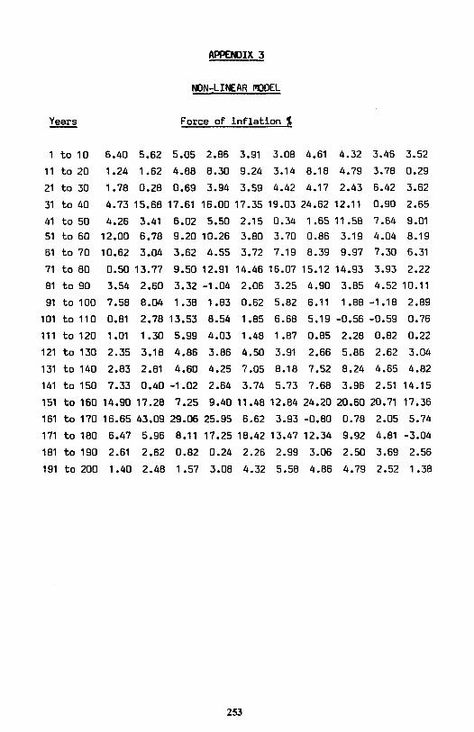
APPENDIX 3

NON-LINEAR MODEL

Force of inflation %

1 to 10 6.40 5.62 5.05 2.86 3.91 3.08 4.61 4.32 3.46 3.52

11 to 20 1.24 1.62 4.88 8.30 9.24 3.14 8.18 4.79 3.78 0.29

21 to 30 1.78 0.28 0.69 3.94 3.59 4.42 4.17 2.43 6.42 3.62

31 to 40 4.73 15.68 17.61 16.00 17.35 19.03 24.62 12.11 0.90 2.65

41 to 50 4.26 3.41 6.02 5.50 2.15 0.34 1.65 11.58 7.64 9.01

51 to 60 12.00 6.78 9.20 10.26 3.80 3.70 0.86 3.19 4.04 8.19

61 to 70 10.62 3.04 3.62 4.55 3.72 7.19 8.39 9.97 7.30 6.31

71 to 80 0.50 13.77 9.50 12.91 14.46 16.07 15.12 14.93 3.93 2.22

81 to 90 3.54 2.60 3.32 -1.04 2.06 3.25 4.90 3.85 4.52 10.11

91 to 100 7.58 8.04 1.38 1.83 0.62 5.82 6.11 1.88 -1.18 2.89

101 to 110 0.81 2.78 13.53 8.54 1.85 6.68 5.19 -0.56 -0.59 0.76

111 to 120 1.01 1.30 5.99 4.03 1.48 1.87 0.85 2.28 0.82 0.22

121 to 130 2.35 3.18 4.86 3.86 4.50 3.91 2.66 5.86 2.62 3.04

131 to 140 2.83 2.81 4.60 4.25 7.05 8.18 7.52 8.24 4.65 4.82

141 to 150 7.33 0.40 -1.02 2.64 3.74 5.73 7.68 3.96 2.51 14.15

151 to 160 14.90 17.28 7.25 9.40 11.48 12.84 24.20 20.60 20.71 17.36

161 to 170 16.65 43.09 29.06 25.95 6.62 3.93 -0.80 0.78 2.05 5.74

171 to 180 6.47 5.96 8.11 17.25 18.42 13.47 12.34 9.92 4.81 -3.04

181 to 190 2.61 2.62 0.82 0.24 2.26 2.99 3.06 2.50 3.69 2.56

191 to 200 1.40 2.48 1.57 3.08 4.32 5.58 4.86 4.79 2.52 1.38

253

Years