Embed Size (px)
Citation preview

HAL Id hal-03018980httpshalarchives-ouvertesfrhal-03018980
Submitted on 24 Nov 2020
HAL is a multi-disciplinary open accessarchive for the deposit and dissemination of sci-entific research documents whether they are pub-lished or not The documents may come fromteaching and research institutions in France orabroad or from public or private research centers
Lrsquoarchive ouverte pluridisciplinaire HAL estdestineacutee au deacutepocirct et agrave la diffusion de documentsscientifiques de niveau recherche publieacutes ou noneacutemanant des eacutetablissements drsquoenseignement et derecherche franccedilais ou eacutetrangers des laboratoirespublics ou priveacutes
A new strategy for the synthesis ofmonomethylhydrazine using the Raschig process 2
Continuous synthesis of stoichiometric monochloramineusing the microreactor technology
Duc Minh Le Anne-Julie Bougrine Olivier Duclos Veacuteronique Pasquet HenriDelalu
To cite this versionDuc Minh Le Anne-Julie Bougrine Olivier Duclos Veacuteronique Pasquet Henri Delalu A new strategyfor the synthesis of monomethylhydrazine using the Raschig process 2 Continuous synthesis ofstoichiometric monochloramine using the microreactor technology Reaction kinetics mechanismsand catalysis Springer 2020 130(1) pp17-34 101007s11144-020-01761-4 hal-03018980
Reaction Kinetics Mechanisms and Catalysis
A new strategy for the synthesis of monomethylhydrazine using the Raschig process 2ndash Continuous synthesis of stoichiometric monochloramine using the microreactor
technology--Manuscript Draft--
Manuscript Number REAC-D-20-00005R1
Full Title A new strategy for the synthesis of monomethylhydrazine using the Raschig process 2ndash Continuous synthesis of stoichiometric monochloramine using the microreactortechnology
Article Type Full Paper
Corresponding Author Veacuteronique PasquetLaboratoire Hydrazines et Composeacutes Energeacutetiques PolyazoteacutesVilleurbanne FRANCE
Corresponding Author SecondaryInformation
Corresponding Authors Institution Laboratoire Hydrazines et Composeacutes Energeacutetiques Polyazoteacutes
Corresponding Authors SecondaryInstitution
First Author Duc Minh Le
First Author Secondary Information
Order of Authors Duc Minh Le
Anne-Julie Bougrine
Olivier Duclos
Veacuteronique Pasquet
Henri Delalu
Order of Authors Secondary Information
Funding Information
Abstract After having established in a previous paper that the synthesis of stoichiometricmonochloramine is hazardous due to the high exothermicity of the reaction and the riskof decomposition of the solution from 36 degC it appeared that the best solution for thissynthesis is to use microreactor technology A series of experiments carried out usinga Doehlert experimental design provided access to a mathematical model describingfor an initial fixed composition ratio [NH4+]0[OCl-]0 the evolution of the yield as afunction of temperature the flow rate of the reagents and the number of sodiumhydroxide equivalent Thus the optimal conditions for the synthesis of stoichiometricchloramine using microreactor technology were established
Response to Reviewers Please find enclosed my answer to your questions(a) The experimental design method makes it possible to reduce the number ofexperiments when there are several parameters to be studied at the same time (hereT eq NaOH flow rate) in order to determine the best conditions for the best result asquickly as possible This is the advantage of a predictive modelThis method is mainly used in industry to quickly determine the most relevantexperiments to be carried out to optimize the conditions of a synthesisb) The microreactor technique using microchannels involves working under pressureto compensate the pressure drop due to the small diameter of the channels Thereforeit is not strictly speaking a pressurized synthesis in a conventional reactor since it is nota conventional reactor The pressure conditions in a microreactor finally allow us toapproach the atmospheric pressure conditions in a conventional reactorTo clarify this point I have added an additional explanation sentence in the paragraph limits of microreactor (highlighting of the added text)
Powered by Editorial Managerreg and ProduXion Managerreg from Aries Systems Corporation
I hope you will be satisfied with these answersYours sincerely
Powered by Editorial Managerreg and ProduXion Managerreg from Aries Systems Corporation
1
A new strategy for the synthesis of monomethylhydrazine using the
Raschig process
2 ndash Continuous synthesis of stoichiometric monochloramine using
the microreactor technology
DM Le A J Bougrine O Duclos V Pasquet H Delalu
Universiteacute Claude Bernard Lyon 1
Laboratoire Hydrazines et Composeacutes Energeacutetiques Polyazoteacutes ndash UMR 5278
UCBLCNRSCNESArianeGroup
Bacirctiment Raulin 2 rue Victor Grignard F-69622 Villeurbanne Cedex France
tel +33 4 72 44 85 47 fax +33 4 72 43 12 91
e-mail veroniquepasquetuniv-lyon1fr
Abstract
After having established in a previous paper that the synthesis of stoichiometric monochloramine is
hazardous due to the high exothermicity of the reaction and the risk of decomposition of the solution
from 36 C it appeared that the best solution for this synthesis is to use microreactor technology A
series of experiments carried out using a Doehlert experimental design provided access to a
mathematical model describing for an initial fixed composition ratio [NH4+]0[OCl-]0 the evolution of
the yield as a function of temperature the flow rate of the reagents and the number of sodium
hydroxide equivalent Thus the optimal conditions for the synthesis of stoichiometric chloramine using
microreactor technology were established
Manuscript Click here to accessdownloadManuscriptREAC-D-20-00005docx
Click here to view linked References
1 2 3 4 5 6 7 8 9 10 11 12 13 14 15 16 17 18 19 20 21 22 23 24 25 26 27 28 29 30 31 32 33 34 35 36 37 38 39 40 41 42 43 44 45 46 47 48 49 50 51 52 53 54 55 56 57 58 59 60 61 62 63 64 65
2
Introduction
In the first part of our study already published(1) we concluded that given the instability of
stoichiometric monochloramine solutions from 36 C and in order to control heat exchanges the
microreactor technology will be the best choice to avoid any sudden degradation leading to the
formation of nitrogen chloride NCl3 Thus this second part studies the optimal conditions for the
synthesis of stoichiometric chloramine using microreactor technology
The development of miniaturized systems known as microsystems has progressed considerably
over the past twenty years(23) More recently these technologies have stimulated the development of
microreactors in the field of process engineering and industries with chemical-related problems With
regard to the synthesis of chloramine under stoichiometric conditions we know that it is highly
exothermic and can easily lead to the formation of explosive by-products (NCl3) Continuous synthesis
with current laboratory equipment therefore presents significant risks For this reason glass
microreactors were used They will permit the study of this continuous synthesis by limiting the
exothermicity of the reaction
Advantages and limitations
Advantages of microreactors
A fundamental property of the microreactor is the high value of the ratio between its surface area and
its volume (specific surface area) For example this value for the Corning microreactor pilot unit used
in this study is 2500 m2m3 with channels with a hydraulic diameter of 07 mm Wall phenomena are
thus intensified In particular heat transfer is significantly increased compared to the other type of
reactors(4) Table 1 shows for example a comparison between different reactor types
Table 1
1 2 3 4 5 6 7 8 9 10 11 12 13 14 15 16 17 18 19 20 21 22 23 24 25 26 27 28 29 30 31 32 33 34 35 36 37 38 39 40 41 42 43 44 45 46 47 48 49 50 51 52 53 54 55 56 57 58 59 60 61 62 63 64 65
3
These transfer characteristics allow for better control and accuracy of operating conditions compared
to conventional reactors In addition parasitic reactions can be avoided by operating within a narrow
window of parameters where the best selectivity is found
The small dimensions of the microreactor system are also of interest mainly in terms of safety due to
the very small volume of product handled This is a considerable advantage for the maintenance and
management of safety in processes involving high-risk compounds (explosive toxic)
Glass microreactors allow easy visualization of phenomena and improved chemical resistance In
general glass is an excellent material for water salt solutions acids and organic compounds(5)
In industrial production micro-reactors make it possible to avoid scale-up operations The transition
from laboratory experiment scale to industrial scale essentially consists in parallelizing the units
(numbering-up) This method makes it possible to avoid the heavy assumptions about extrapolation
factors as well as the risks intrinsic to any change in scale (degradation of product quality loss of energy
performance hydrodynamic dysfunctions etc)(4)
Limits of microreactors
Microreactors are limited by the laws of hydrodynamics Indeed the miniaturization of the channels
inevitably leads to an increase in pressure drop In order to compensate this pressure drop it is
necessary to work under pressure to have a sufficient flow in the channels On the laboratory
microreactor unit the pressure is in the range of 7 to 10 bar for flows ranging from 80 to 120 mL min-
1 On the other hand glass remains very fragile in the face of mechanical stresses and strains Synthesis
is therefore limited to pressures below 20 bar with a maximum total flow rate of 200 mL min-1
For continuous use of microreactors at the industrial level the passage of reagents will lead to
progressive fouling of the microchannels They will therefore have a limited operating time which will
vary depending on the reagents used and the products formed during the synthesis This pollution will
1 2 3 4 5 6 7 8 9 10 11 12 13 14 15 16 17 18 19 20 21 22 23 24 25 26 27 28 29 30 31 32 33 34 35 36 37 38 39 40 41 42 43 44 45 46 47 48 49 50 51 52 53 54 55 56 57 58 59 60 61 62 63 64 65
4
therefore require a special cleaning protocol and possibly in the long term a replacement cycle for
microreactor modules
Experimental part
Corning microreactor
The study of the continuous synthesis of stoichiometric monochloramine was performed on the
Corning microreactor unit shown in Fig 1
The different elements of the Corning microreactor unit are as follows
- 2 DTR microstructures pre-cooling plates
- 1 MFA microstructure separation of the bleach supply into 4 streams
- 1 MJ microstructure reaction plate composed of 4 mixing zones
For each structure the experimental conditions are as follows
DTR microstructure Vreagent 9 mL Vheat exchange 14 mL Sexchange 17500 mmsup2 ΔP 100 mbar
MFA microstructure Vreagent 1 mL Vheat exchange 13 mL Sexchange 3000 mmsup2
MJ microstructure Vreagent 10 mL Vheat exchange 16 mL Sexchange 23500 mmsup2 ΔP 2500 mbar
with Sexchange heat exchange surface of the microstructure (mm2)
and ΔP pressure drop in the microstructure (mbar) (Pressure drops are measured with water at a flow
rate of 100 mL min-1 and at 20 C)
The so-called microreactor part is composed of 4 glass modules The 2 DTR modules are designed to
pre-cool the reagents at different temperatures The MFA module is a manifold that divides the bleach
supply into 4 streams of equal flow rates The MJ module is the reaction module with 4 mixing zones
1 2 3 4 5 6 7 8 9 10 11 12 13 14 15 16 17 18 19 20 21 22 23 24 25 26 27 28 29 30 31 32 33 34 35 36 37 38 39 40 41 42 43 44 45 46 47 48 49 50 51 52 53 54 55 56 57 58 59 60 61 62 63 64 65
5
It provides mixing and residence time actions at each injection point The hydraulic diameter of the
channels in the glass modules is 07 mm (manufacturers data) The fluid flow regime in the
microreactor unit is therefore laminar (Reynolds number is less than 104)
In order to overcome the laminar regime obstacles are created in the MJ microstructure plate (Fig 2)
These obstacles aim to break the flow and create a turbulent flow which means better heat exchange
and better mixing action
Temperature control is provided by Lauda Integral T 2200 thermostats with 27 kW cryogenic power
They allow working in a temperature range from -25 C to 120 C Reagent flow is controlled with two
HNP Mikrosysteme Mzr-7259Ex gear pumps (PP1 PP2) and two ROTAMASS series 3 Coriolis mass
flowmeters (FM1 FM2) supplied by Yokogawa Sensors T1 T2 T3 and P1 P2 P3 are used to monitor
the temperature and pressure of the fluids before and after reaction as well as the system pressure
drops as a function of the fluid flows
Chemical products
The permuted water used is city water purified by passing over an ion exchange resin The inorganic
salts and organic solvents used are of commercial purity (minimum 98) and are supplied by Acros
Organics Merck and Sigma-Aldrich They were used without prior purification unless otherwise
indicated Aqueous solutions of sodium hypochlorite NaOCl and sodium hydroxide are supplied by
Arkema (Jarrie Plant Grenoble France) The aqueous solution measuring approximately 48
chlorometric degrees (24 mol L-1) is stored at 5 C and systematically titrated before use
Analytical methods
Iodometric dosage
1 2 3 4 5 6 7 8 9 10 11 12 13 14 15 16 17 18 19 20 21 22 23 24 25 26 27 28 29 30 31 32 33 34 35 36 37 38 39 40 41 42 43 44 45 46 47 48 49 50 51 52 53 54 55 56 57 58 59 60 61 62 63 64 65
6
This method was used to determine the active chlorine concentrations of chloramine solutions and
hypochlorite ions It is based on the oxidation of potassium iodide in acetic medium with titration of
iodine released by a 01 M sodium thiosulfate solution The dosing reaction was monitored by
potentiometry using a Metrohm 60451100 combined platinum electrode
UV spectrometry
The spectrophotometer used was an Agilent Cary 100 dual beam spectrophotometer equipped with
the Cary WinUV data acquisition system It allows a repetitive scanning of spectra between 180 nm
and 900 nm programmable as a function of time and measurements of optical density or its
derivatives at a given wavelength Measurements were made with Hellmareg brand Suprasilreg quartz
cells model 100-QS with a 10 mm optical path to ensure optimal transmission of UV signals
Continuous chloramine synthesis
Between two manipulations an isopropanol solution is injected into the device to ensure proper
preservation of the pumps and glass microstructures The rinsing solution used to purge and clean the
installation is then a mixture of 25 water and 75 ethanol
The reagent solutions (NH4Cl solution and alkaline bleach solution) are previously prepared and cooled
(generally -5 C) Before each synthesis experiment a waterethanol solution is circulated at the
desired flow rate to remove isopropanol from the pipes Once the isopropanol has been purged NH4Cl
is introduced and then bleach The synthesis is carried out for all experiments under a pressure of 11
bar During normal operation the steady state is reached after 10 min Samples are then taken
punctually every 15 min then analyzed by iodometric dosage and UV - Visible spectrometry
Measurements of temperature fluid density and pressure are carried out online at different points in
the installation in order to check that the synthesis is proceeding correctly and to make an immediate
correction in the event of significant deviations from the instructions A pH monitoring at the end of
the reaction module is necessary to avoid any drift of the monochloramine solutions Indeed a pH
1 2 3 4 5 6 7 8 9 10 11 12 13 14 15 16 17 18 19 20 21 22 23 24 25 26 27 28 29 30 31 32 33 34 35 36 37 38 39 40 41 42 43 44 45 46 47 48 49 50 51 52 53 54 55 56 57 58 59 60 61 62 63 64 65
7
below 10 leads to the potential formation of highly explosive dichloramine NHCl2 and nitrogen
trichloride NCl3
At the end of the synthesis the microreactor unit is rinsed with a waterethanol solution for 30 min
then an isopropanol solution is injected to preserve the pumps and microstructures
Results and discussion
Experimental design
Experimental design method
Throughout this study on the Corning microreactor unit many parameters that could influence the
synthesis were investigated The classical experimental methodology consists of setting the level of all
but one of the variables and measuring the system response for different values of this variable which
implies carrying out a considerable number of experiments For example for 4 variables at 4 levels (ie
using 4 different values for each variable) 44 = 256 experiments must be performed In order to avoid
too many experiments the design of experiments method was used
Indeed the designs of experiments are derived from mathematical and statistical methods applied to
experimentation The principle of this technique is to simultaneously vary the levels of one or more
factors (discrete or continuous variables) in each experiment This will significantly reduce the number
of experiments to be carried out while increasing the number of factors studied detecting the
interactions between the different factors and a given response ie a quantity used as a criterion and
allowing the results to be modelled It should be noted that the main difference with the traditional
method is that the design of experiments method allows the levels of all factors to be varied at the
same time for each experiment in a programmed and reasoned way(6)
For this study the factors studied were
- the number of soda equivalent in bleach
1 2 3 4 5 6 7 8 9 10 11 12 13 14 15 16 17 18 19 20 21 22 23 24 25 26 27 28 29 30 31 32 33 34 35 36 37 38 39 40 41 42 43 44 45 46 47 48 49 50 51 52 53 54 55 56 57 58 59 60 61 62 63 64 65
8
- the temperature of the reagents (bleach and NH4Cl solution)
- the flow of fluids
- the pressure
Complete factorial plan 23
First the most influential factors governing the system response will be sought rather than a specific
relationship between factor variations and response variations Previous studies in the laboratory have
shown a significant influence of the amount of soda present in bleach on the monochloramine yield of
the synthesis(7) The influence of the remaining three factors (temperature flow and pressure)
therefore remains to be quantified
To this end a complete factorial design with these three factors (temperature flow rate and pressure)
was used due to its simplicity and speed of implementation This method consists of performing the
experiments by varying the factors between a high (+) and low (-) level In this case this plan is rated
23 (3 factors with 2 levels each) and therefore includes 8 experiments The numerical values of the 2
levels of each of the 3 factors and the associated response (monochloramine yield) are given in Table
2
Table 2
The mathematical model associated with the complete plan 23 is as follows
y = a0 + a1x1 + a2x2 + a3x3 + a12x1x2 + a13x1x3 + a23x2x3+ a123x1x2x3
with
y the answer (in this case the yield of the synthesis)
xi the abscissa of the experimental point for factor i Given the levels that the factors take xi takes the
value 1 for level (+) and -1 for level (-)
1 2 3 4 5 6 7 8 9 10 11 12 13 14 15 16 17 18 19 20 21 22 23 24 25 26 27 28 29 30 31 32 33 34 35 36 37 38 39 40 41 42 43 44 45 46 47 48 49 50 51 52 53 54 55 56 57 58 59 60 61 62 63 64 65
9
a0 the value of the response at the center of the field of study
ai the effect of factor i
aij the interaction between factors i and j (the same for a123 which is the interaction between the three
factors)
The coefficients of the model can be determined using the following matrix equation
1 1 1 1 1 1 1 1
1 -1 1 1 -1 -1 1 -1
1 1 -1 1 -1 1 -1 -1
1 1 1 -1 1 -1 -1 -1
1 -1 -1 1 1 -1 -1 1
1 -1 1 -1 -1 1 -1 1
1 1 -1 -1 -1 -1 1 1
1 -1 -1 -1 1 1 1 -1
1
2
3
4
5
6
7
8
y
y
y
y
y
y
y
y
0
1
2
3
12
13
23
123
a
a
a
a
a
a
a
a
then in condensed form
y =Xsdota
with
y column matrix containing the eight answers
X effects calculation matrix This matrix is composed of the values taken by the levels of different
factors or the products of the coordinates of these factors(8)
a column matrix of the coefficients of the mathematical model
1 2 3 4 5 6 7 8 9 10 11 12 13 14 15 16 17 18 19 20 21 22 23 24 25 26 27 28 29 30 31 32 33 34 35 36 37 38 39 40 41 42 43 44 45 46 47 48 49 50 51 52 53 54 55 56 57 58 59 60 61 62 63 64 65
10
The values of the coefficients of the model are obtained by solving the matrix equation
The effects of the different factors and their interactions are shown in Fig 3
To conclude Fig 3 shows that among these three factors the most influential are in order of
importance temperature and flow rate Pressure is not a decisive parameter These factors will now
be addressed in a Doehlert plan
Composite plan of Doehlert
The combination of all the results shows that the factors that have the most influence on the yield of
monochloramine synthesis are the amount of NaOH in bleach temperature and fluid flow Pressure
has very little influence and is therefore now set for all experiments at 11 bar a value similar to that
of the installations at the industrial ArianeGroup site in Toulouse (France)
In order to study the effects of these three factors on performance a Doehlert plan of experiments is
established because of its advantages over factor designs The first advantage of Doehlert plan is that
each factor now has several levels (instead of 2 as in factorial plan 23) The number of levels for each
factor is variable which allows the operator flexibility to assign a large number of levels or not to a
factor In this study the number of soda equivalent factor was chosen as the factor with the highest
1 2 3 4 5 6 7 8 9 10 11 12 13 14 15 16 17 18 19 20 21 22 23 24 25 26 27 28 29 30 31 32 33 34 35 36 37 38 39 40 41 42 43 44 45 46 47 48 49 50 51 52 53 54 55 56 57 58 59 60 61 62 63 64 65
11
number of levels in order to obtain the maximum information from the system Finally the
representative points of the different experiments in the Doehlert plan are placed according to a
geometric figure which ensures that the experiments are regularly placed in the experimental space(8)
Fig 4 shows schematically the distribution of experiments for a three-factor Doehlert plan
The postulated mathematical model used with Doehlert plan is a second degree equation
y = a0 + a1x1 + a2x2 + a3x3 + a12x1x2 + a13x1x3 + a23x2x3 + a11x12 + a22x2
2 + a33x32
with
Y the answer (in our case the yield of the synthesis)
Xi the abscissa of the experimental point for factor i in coded coordinates (Table 3)
ai aij coefficient of the mathematical model
The parameters of the plan experiments and the experimental results are shown in Table 3
Table 3
In this case the calculation matrix is a 15 times 10 matrix since there are 15 experiments and 10 coefficients
in the mathematical model These coefficients are calculated by the following formula(8)
a =(XTX)ndash1XTy
with
a vector of coefficients
X calculation matrix (XT matrix transposed from X)
y vector of experiment results
After solving the matrix equation the mathematical model is as follows
y = 9773 ndash 1642x1 ndash 4003x2 ndash 3505x3 + 39193x1x2 ndash 12883x1x3 ndash 6568x2x3 + 0030x12 ndash 40578x2
2 ndash
4770x32
Table 4 shows the experimental and modelled results for each experiment performed
1 2 3 4 5 6 7 8 9 10 11 12 13 14 15 16 17 18 19 20 21 22 23 24 25 26 27 28 29 30 31 32 33 34 35 36 37 38 39 40 41 42 43 44 45 46 47 48 49 50 51 52 53 54 55 56 57 58 59 60 61 62 63 64 65
12
Table 4
The overall quality of the adjusted mathematical model is assessed using the following two statistical
tools(9)
- Fisher test
This test aims to reject the hypothesis (H0) that the model does not describe the variation of the tests
When this hypothesis is verified it is shown that the statistic Fregression described by the relationship
below follows a Fisher law with Xν and
Rν degrees of freedom(10)
Xν and
Rν are the numbers of
degrees of freedom associated respectively with the sum of the squares of deviations from the
regression average value and the sum of the squares of the residues
2
i
reacutegression 2
i i
y -yF =
ˆy -y
with
y average value of experimental results
yi experimental value for experiment number i
y i value calculated from the model for experiment number i
Thus this hypothesis is rejected with a probability α if
Fregression gt F(α Xν
Rν )
Here F(α Xν
Rν ) is the (1 - α) quantile of a Fisher law with
Xν and
Rν degrees of freedom
- Coefficient of determination Rsup2 of the multilinear regression
This coefficient is defined by the ratio of the dispersion of the results explained by the model to the
total dispersion of the results
1 2 3 4 5 6 7 8 9 10 11 12 13 14 15 16 17 18 19 20 21 22 23 24 25 26 27 28 29 30 31 32 33 34 35 36 37 38 39 40 41 42 43 44 45 46 47 48 49 50 51 52 53 54 55 56 57 58 59 60 61 62 63 64 65
13
2
i2
2
i
y -yR =
y -y
When Rsup2 = 1 the estimations by the mathematical model coincide with the measurements while for
Rsup2 = 0 the data are not at all aligned The value of Rsup2 in this case is 098 which means that 98 of the
variation in the experiments is explained by the mathematical model
The experimental results lead to Table 5
According to Table 5 the statistic Fregression satisfies the Fisher test with a 95 confidence level This
mathematical model therefore makes it possible to describe the response of the experiments in a
satisfactory way
- Canonical analysis
The mathematical model associated with Doehlert plan is a second order polynomial model so a
canonical analysis can be performed This technique allows to easily deduce the essential
characteristics of the model such as the coordinates of the stationary point of the model and the
associated response the type of the stationary point (maximum minimum minimax) the main axes
as well as the variation of the model relative to each of these axes(11) To do this the mathematical
model was written in the following matrix form
y = a0 + xT b + xTBx
1 2 3 4 5 6 7 8 9 10 11 12 13 14 15 16 17 18 19 20 21 22 23 24 25 26 27 28 29 30 31 32 33 34 35 36 37 38 39 40 41 42 43 44 45 46 47 48 49 50 51 52 53 54 55 56 57 58 59 60 61 62 63 64 65
14
with
The matrix equation of the second degree model implicitly implies the existence of a so-called
stationary point S (unique) for which the partial derivatives of the response with respect to variables
xi are all zero Thus
y0
x
wich gives
1S
1
2
x B b and T 1S 0
1y a
4
b B b
The stationary point is therefore
xS =
048
-021
-064
temperature = 157 C
= eq NaOH = 021 equivalent
flow rate = 44 mL min-1
and yS = 10249
a1
b = a2
a3
x1
x = x2
x3
-267
= 369
011
a11 frac12 a12 frac12a13 -047 984 -392
B = frac12a12 a22 frac12a23 = 984 -2688 -492
frac12a13 frac12a23 a33 -392 -492 -637
1 2 3 4 5 6 7 8 9 10 11 12 13 14 15 16 17 18 19 20 21 22 23 24 25 26 27 28 29 30 31 32 33 34 35 36 37 38 39 40 41 42 43 44 45 46 47 48 49 50 51 52 53 54 55 56 57 58 59 60 61 62 63 64 65
15
A significant simplification can be achieved if the mathematical model is seen from a particular
benchmark translated and returned relative to the original benchmark (factor benchmark xi) To do
this first of all the axes of the original reference frame will be rotated around its origin The purpose
of this operation is to remove the interaction monomas between factors xi Once the rotation is
completed a translation will allow the removal of the first order terms from the polynomial model
Fig 5 shows for example the position of the axes during these operations
The objective of this transformation is to bring the model back to the following canonical form
y = yS + λ1z12 + λ2z2
2 +λ3z32
with
y the response of the model (in this case the yield of the synthesis)
zi the ith coordinates of the experimental point in the final reference frame
yS the response at the stationary point S
λi the eigenvalues of matrix B
To do this matrix B must be transformed into a diagonal matrix The notions of vectors and eigenvalues
then come into play We will note Θ the diagonal matrix whose element Θii is the eigenvalue λi of B
1
2
3
0 0
0 0
0 0
Θ
In the final reference frame the mathematical model will therefore be written in the following matrix
form
1 2 3 4 5 6 7 8 9 10 11 12 13 14 15 16 17 18 19 20 21 22 23 24 25 26 27 28 29 30 31 32 33 34 35 36 37 38 39 40 41 42 43 44 45 46 47 48 49 50 51 52 53 54 55 56 57 58 59 60 61 62 63 64 65
16
y = yS + zTΘz
Similarly the matrix is defined by M for which the ith column is the ith eigenvector of B This matrix M
plays an important role since it allows the passage of the coordinates of the experimental point in the
original reference frame x =[x1 x2 x3]T to the coordinates z =[z1 z2 z3]T in the final reference frame
and vice-versa
z = MT(x ndash xS)
x = xS + Mz
The numerical results in the case of this mathematical model are presented
Θ =
and M =
The unit vectors of the final reference frame expressed in coordinates of the original reference frame
with their associated eigenvalues are
λ1 = ndash48502 λ2 = 11195 λ3 = ndash8012
-3065 0 0
0 525 0
0 0 -832
02898 -08464 04467
-09461 -03239 -00001
-01448 04226 08947
02898 -08464 04467
z1 = -09461 z2 = -03239 z3 = -00001
-01448 04226 08947
1 2 3 4 5 6 7 8 9 10 11 12 13 14 15 16 17 18 19 20 21 22 23 24 25 26 27 28 29 30 31 32 33 34 35 36 37 38 39 40 41 42 43 44 45 46 47 48 49 50 51 52 53 54 55 56 57 58 59 60 61 62 63 64 65
17
The mathematical model is therefore written
y = 9809 ndash 48502z12 + 11195z2
2 ndash 8012z32
2 eigenvalues are negative (λ1 and λ3) and one eigenvalue is positive (λ2) The response y decreases on
axes z1 and z3 with negative eigenvalues but increases on axis z2 The order of magnitude of the
coefficients is also important Indeed for the same variation of the zi component of z its effect will be
all the greater if the corresponding coefficient (λi) is great On the other hand this effect will be all the
less important if its coefficient is small Fig 6 shows the effects of changes of the zi components
Fig 7 visually shows the relative positions of the unit vectors of the original (xi) and final (zi) landmarks
The canonical analysis that has been carried out shows that to increase the response y (the yield of
monochloramine synthesis) it is necessary to move away from the stationary point S along the z2 axis
(whose associated eigenvalue λ2 is positive) 2 points are considered P1 =[0 1 0]marker z and P2 =[0 -1
0]marker z These two points therefore correspond to the following two experimental conditions
1 2 3 4 5 6 7 8 9 10 11 12 13 14 15 16 17 18 19 20 21 22 23 24 25 26 27 28 29 30 31 32 33 34 35 36 37 38 39 40 41 42 43 44 45 46 47 48 49 50 51 52 53 54 55 56 57 58 59 60 61 62 63 64 65
18
Point P2 is rejected because of its high reagent temperature The temperature of the chloramine
solution at the outlet of the unit is therefore necessarily below 20 C This high temperature strongly
favours the degradation of the solution and can potentially cause a sudden or even rapid degradation
of the synthesis For safety reasons point P1 is adopted as the optimal conditions for the synthesis of
stoichiometric chloramine on the microreactor unit
Conclusion
For the first time the use of microreactors allows the continuous preparation of stoichiometric
monochloramine Under the experimental conditions studied the study of the synthesis of NH2Cl on
the microreactor pilot unit allows to conclude that
- the total flow rate has very little influence on reaction performance
- two parameters have a decisive influence on the reaction performance namely the temperature and
the number of sodium equivalent in bleach
- an excess of sodium hydroxide gradually leads to a drop in the initially almost quantitative yield from
97 to 84 This is due to a substitution reaction of Cl- by OH- with transient formation of
-036 temperature = 22 C
P1 = -053 = eqNaOH = 013 equivalent
-022 marker x flow rate = 546 mL min-1
133 temperature = 293 C
P2 = 012 = eqNaOH = 029 equivalent
-106 marker x flow rate = 335 mL min-1
1 2 3 4 5 6 7 8 9 10 11 12 13 14 15 16 17 18 19 20 21 22 23 24 25 26 27 28 29 30 31 32 33 34 35 36 37 38 39 40 41 42 43 44 45 46 47 48 49 50 51 52 53 54 55 56 57 58 59 60 61 62 63 64 65
19
hydroxylamine The number of sodium equivalent does not exceed 025 to obtain a quasi-quantitative
yield
The lower bound of number of sodium equivalent is strongly influenced by temperature Generally
speaking if the number of sodium equivalent is equal to 005 a lower yield at 86 (T = 0 C) is observed
which is aggravated by a rise in temperature
The major safety parameter is the initial concentration of sodium hydroxide in bleach Whatever the
temperature this parameter must in all cases be higher than the minimum of 01 preferably for
safety reasons at 02-025 Under these conditions it is possible to carry out the synthesis preferably
between 0 and 24 C
To ensure process safety it would be necessary to continuously measure the pH of the chloramine
solution downstream of the reactor andor perform an online UV measurement to verify the
conformity of the absorption spectrum
After discussion with our industrial partner and taking into account process safety aspects we
therefore recommend the following conditions for the synthesis of stoichiometric chloramine
Temperature 0 C
NaOH equivalent 020 eq
Reagent flow rate 50 mL min-1
Pressure 11 bar
1 2 3 4 5 6 7 8 9 10 11 12 13 14 15 16 17 18 19 20 21 22 23 24 25 26 27 28 29 30 31 32 33 34 35 36 37 38 39 40 41 42 43 44 45 46 47 48 49 50 51 52 53 54 55 56 57 58 59 60 61 62 63 64 65
20
Bibliography
(1) Le D M Bougrine A J Pasquet V Delalu H (2019) A new strategy for the synthesis of
monomethylhydrazine using the Raschig process 1 Study of the stability of monochloramine React
Kinet Catal 127(2) 757-773
(2) Ehrfeld W Hessel V Loumlwe H (2000) Microreactors ndash New Technology for Modern Chemistry 1st ed
Wiley VCH Mainz
(3) Hessel V Hardt S Loumlve H (2004) Chemical Micro Process Engineering ndash Fundamentals Modelling
and Reactions Wiley VCH Mainz
(4) Aubin J Xuereb C (2008) Microreacuteacteurs pour lrsquoindustrie Base documentaire Deacuteveloppement de
solvants alternatifs et intensification des proceacutedeacutes Techniques de lrsquoingeacutenieur Ref IN94
(5) Frank T (2008) Microreactors in Organic Synthesis and Catalysis Wiley VCH Weinheim
(6) Goupy J (2001) Introduction aux plans drsquoexpeacuteriences 2nd ed Dunod Paris
(7) Delalu H Duriche C Berthet J Le Gars P (2006) Process for the synthesis of monochloramine US
Patent 7045659
(8) Goupy J (1999) Plans drsquoexpeacuteriences pour surfaces de reacuteponse Dunod Paris
(9) Kamoun A Chaabouni M M Ayedi H F (2011) Plans drsquoexpeacuteriences et traitement de surface ndash
Meacutethodologie des surfaces de reacuteponses Base documentaire Traitements de surface des meacutetaux
contexte et gestion environnementale Technique de lrsquoingeacutenieur Ref M1429
(10) Dodge Y Rousson V (2004) Analyse de reacutegression appliqueacutee Dunod Paris
(11) Brisset S Gillon F Vivier S Brochet P (2001) Optimization with experimental design an approach
using Taguchirsquos methodology and finite element simulations IEEE Transactions on magnetics 37(5)
3530-3533
1 2 3 4 5 6 7 8 9 10 11 12 13 14 15 16 17 18 19 20 21 22 23 24 25 26 27 28 29 30 31 32 33 34 35 36 37 38 39 40 41 42 43 44 45 46 47 48 49 50 51 52 53 54 55 56 57 58 59 60 61 62 63 64 65
21
(12) Lavric E D (2008) Thermal performance of Corning glass microstructures Conference ECI
International Conference on Heat Transfer and Fluid Flow in Microscale Whistler
1 2 3 4 5 6 7 8 9 10 11 12 13 14 15 16 17 18 19 20 21 22 23 24 25 26 27 28 29 30 31 32 33 34 35 36 37 38 39 40 41 42 43 44 45 46 47 48 49 50 51 52 53 54 55 56 57 58 59 60 61 62 63 64 65
22
Table 1 Comparison table of current exchange modules(12)
Module Specific area m2m3
Volumetric thermal transfer coefficient
MWm3sdotK
Batch reactor
25 10-3
Batch reactor with exchanger
10 10-2
Tubular exchanger
400 02
Plate heat exchanger
800 125
Glass Corning microstructure
2500 17
1 2 3 4 5 6 7 8 9 10 11 12 13 14 15 16 17 18 19 20 21 22 23 24 25 26 27 28 29 30 31 32 33 34 35 36 37 38 39 40 41 42 43 44 45 46 47 48 49 50 51 52 53 54 55 56 57 58 59 60 61 62 63 64 65
23
Table 2 Plan 23 experience Matrix summary of the experiments
Experiment number
Factor 1 Factor 2 Factor 3 Answer Temperature Flow rate Pressure NH2Cl Yield ()
1 + + + 869
2 ndash + + 990
3 + ndash + 860
4 + + ndash 926
5 ndash ndash + 995
6 ndash + ndash 990
7 + ndash ndash 832
8 ndash ndash ndash 986
Effective values C mL min-1 bar
Level (+) 30 100 16
Level (ndash) -10 30 7
1 2 3 4 5 6 7 8 9 10 11 12 13 14 15 16 17 18 19 20 21 22 23 24 25 26 27 28 29 30 31 32 33 34 35 36 37 38 39 40 41 42 43 44 45 46 47 48 49 50 51 52 53 54 55 56 57 58 59 60 61 62 63 64 65
24
Table 3 Doehlert plan for three factors summary of experimental tests
Experiment number
Factor 1 Factor 2 Factor 3 Temperature Soda equivalent Flow rate
Encoded value
Real value Encoded
value Real value
Encoded value
Real value
C mL minndash1
1 0 8 0 026 0 60
2 1 24 0 026 0 60
3 05 16 0866 047 0 60
4 -05 0 -0866 005 0 60
5 -1 -8 0 026 0 60
6 -05 0 -0866 005 0 60
7 05 16 -0866 005 0 60
8 0 8 0 026 0 60
9 -05 0 0289 033 0816 80
10 0 8 -0577 012 0816 80
11 05 16 0289 033 0816 80
12 -05 0 -0289 019 -0816 40
13 0 8 0577 040 -0816 40
14 05 16 -0289 019 -0816 40
15 0 8 0 026 0 60
Level ndash1 -8 002 35
Level 0 8 026 60
Level +1 24 050 85
119821 119809 0866 =radic3
2 0816 =
radic2
radic3 0577 =
1
radic3 0289 =
1
2radic3
1 2 3 4 5 6 7 8 9 10 11 12 13 14 15 16 17 18 19 20 21 22 23 24 25 26 27 28 29 30 31 32 33 34 35 36 37 38 39 40 41 42 43 44 45 46 47 48 49 50 51 52 53 54 55 56 57 58 59 60 61 62 63 64 65
25
Table 4 Results of the Doehlert plan experiments
Experiment number
Experimental yield ()
Modelled yield ()
1 9773 9773
2 9996 9940
3 8338 8163
4 8419 8692
5 9556 9612
6 879 8692
7 5462 5462
8 9773 9773
9 8495 8439
10 8532 8357
11 8452 8683
12 9553 9322
13 8292 8467
14 9351 9407
15 9773 9773
1 2 3 4 5 6 7 8 9 10 11 12 13 14 15 16 17 18 19 20 21 22 23 24 25 26 27 28 29 30 31 32 33 34 35 36 37 38 39 40 41 42 43 44 45 46 47 48 49 50 51 52 53 54 55 56 57 58 59 60 61 62 63 64 65
26
Table 5 Fisher test for regression
Source of variation
Degree of liberty
Sum of the squares
Expression Fregression F(095 9 5) Rsup2
Total 15 ndash 1 177370 2
iy -y
59 4772 098 Regression 10 ndash 1 174420 2
iy -y
residual 15 ndash 10 2952 2
i iy -y
1 2 3 4 5 6 7 8 9 10 11 12 13 14 15 16 17 18 19 20 21 22 23 24 25 26 27 28 29 30 31 32 33 34 35 36 37 38 39 40 41 42 43 44 45 46 47 48 49 50 51 52 53 54 55 56 57 58 59 60 61 62 63 64 65
27
Fig 1 Diagram of the Corning microreactor pilot unit
Cooling
system
Cooling
system
Bleach
Sample Release
Release
Waterethanol
1 2 3 4 5 6 7 8 9 10 11 12 13 14 15 16 17 18 19 20 21 22 23 24 25 26 27 28 29 30 31 32 33 34 35 36 37 38 39 40 41 42 43 44 45 46 47 48 49 50 51 52 53 54 55 56 57 58 59 60 61 62 63 64 65
28
Fig 2 Structure created in the MJ microstructure unit to break the flow
mixer Structure created to break the flow
Turbulent flow
MJ microstructure
temperature-
controlled fluid
reagents Product
1 2 3 4 5 6 7 8 9 10 11 12 13 14 15 16 17 18 19 20 21 22 23 24 25 26 27 28 29 30 31 32 33 34 35 36 37 38 39 40 41 42 43 44 45 46 47 48 49 50 51 52 53 54 55 56 57 58 59 60 61 62 63 64 65
29
Fig 3 Coefficients of the mathematical model of the plan 23
-60
-50
-40
-30
-20
-10
00
10
20
30
a1 a2 a3 a12 a13 a23 a123
Co
effi
cien
t va
lue
Temperature
Flow rate
Pressure
1 2 3 4 5 6 7 8 9 10 11 12 13 14 15 16 17 18 19 20 21 22 23 24 25 26 27 28 29 30 31 32 33 34 35 36 37 38 39 40 41 42 43 44 45 46 47 48 49 50 51 52 53 54 55 56 57 58 59 60 61 62 63 64 65
30
Fig 4 Arrangement of Doehlert plan points for 3 factors
Factor 1 Factor 2
Factor 3
Temperature Soda equivalent
Flow rate
1 2 3 4 5 6 7 8 9 10 11 12 13 14 15 16 17 18 19 20 21 22 23 24 25 26 27 28 29 30 31 32 33 34 35 36 37 38 39 40 41 42 43 44 45 46 47 48 49 50 51 52 53 54 55 56 57 58 59 60 61 62 63 64 65
31
Fig 5 Position of the axes during the transformation operations (a) original position (original axes)
(b) positions of the axes during rotation (c) position of the axes during translation
(a) (b) (c)
1 2 3 4 5 6 7 8 9 10 11 12 13 14 15 16 17 18 19 20 21 22 23 24 25 26 27 28 29 30 31 32 33 34 35 36 37 38 39 40 41 42 43 44 45 46 47 48 49 50 51 52 53 54 55 56 57 58 59 60 61 62 63 64 65
32
Fig 6 Variations of the response y according to the axes zi
400
600
800
1000
-1 -075 -05 -025 0 025 05 075 1
value zi
y
z1
z2
z3
1 2 3 4 5 6 7 8 9 10 11 12 13 14 15 16 17 18 19 20 21 22 23 24 25 26 27 28 29 30 31 32 33 34 35 36 37 38 39 40 41 42 43 44 45 46 47 48 49 50 51 52 53 54 55 56 57 58 59 60 61 62 63 64 65
33
Fig 7 Relative positions of the unit vectors of the original and final landmarks (views taken from
different angles)
X1
X1
X1
X1
X2 X2
X2
X2
X3 X3
X3 X3
Z1
Z1
Z1
Z1
Z2
Z2
Z2
Z2
Z3
Z3
Z3
Z3
1 2 3 4 5 6 7 8 9 10 11 12 13 14 15 16 17 18 19 20 21 22 23 24 25 26 27 28 29 30 31 32 33 34 35 36 37 38 39 40 41 42 43 44 45 46 47 48 49 50 51 52 53 54 55 56 57 58 59 60 61 62 63 64 65

1
A new strategy for the synthesis of monomethylhydrazine using the
Raschig process
2 ndash Continuous synthesis of stoichiometric monochloramine using
the microreactor technology
DM Le A J Bougrine O Duclos V Pasquet H Delalu
Universiteacute Claude Bernard Lyon 1
Laboratoire Hydrazines et Composeacutes Energeacutetiques Polyazoteacutes ndash UMR 5278
UCBLCNRSCNESArianeGroup
Bacirctiment Raulin 2 rue Victor Grignard F-69622 Villeurbanne Cedex France
tel +33 4 72 44 85 47 fax +33 4 72 43 12 91
e-mail veroniquepasquetuniv-lyon1fr
Abstract
After having established in a previous paper that the synthesis of stoichiometric monochloramine is
hazardous due to the high exothermicity of the reaction and the risk of decomposition of the solution
from 36 C it appeared that the best solution for this synthesis is to use microreactor technology A
series of experiments carried out using a Doehlert experimental design provided access to a
mathematical model describing for an initial fixed composition ratio [NH4+]0[OCl-]0 the evolution of
the yield as a function of temperature the flow rate of the reagents and the number of sodium
hydroxide equivalent Thus the optimal conditions for the synthesis of stoichiometric chloramine using
microreactor technology were established
Manuscript Click here to accessdownloadManuscriptREAC-D-20-00005docx
Click here to view linked References
1 2 3 4 5 6 7 8 9 10 11 12 13 14 15 16 17 18 19 20 21 22 23 24 25 26 27 28 29 30 31 32 33 34 35 36 37 38 39 40 41 42 43 44 45 46 47 48 49 50 51 52 53 54 55 56 57 58 59 60 61 62 63 64 65
2
Introduction
In the first part of our study already published(1) we concluded that given the instability of
stoichiometric monochloramine solutions from 36 C and in order to control heat exchanges the
microreactor technology will be the best choice to avoid any sudden degradation leading to the
formation of nitrogen chloride NCl3 Thus this second part studies the optimal conditions for the
synthesis of stoichiometric chloramine using microreactor technology
The development of miniaturized systems known as microsystems has progressed considerably
over the past twenty years(23) More recently these technologies have stimulated the development of
microreactors in the field of process engineering and industries with chemical-related problems With
regard to the synthesis of chloramine under stoichiometric conditions we know that it is highly
exothermic and can easily lead to the formation of explosive by-products (NCl3) Continuous synthesis
with current laboratory equipment therefore presents significant risks For this reason glass
microreactors were used They will permit the study of this continuous synthesis by limiting the
exothermicity of the reaction
Advantages and limitations
Advantages of microreactors
A fundamental property of the microreactor is the high value of the ratio between its surface area and
its volume (specific surface area) For example this value for the Corning microreactor pilot unit used
in this study is 2500 m2m3 with channels with a hydraulic diameter of 07 mm Wall phenomena are
thus intensified In particular heat transfer is significantly increased compared to the other type of
reactors(4) Table 1 shows for example a comparison between different reactor types
Table 1
1 2 3 4 5 6 7 8 9 10 11 12 13 14 15 16 17 18 19 20 21 22 23 24 25 26 27 28 29 30 31 32 33 34 35 36 37 38 39 40 41 42 43 44 45 46 47 48 49 50 51 52 53 54 55 56 57 58 59 60 61 62 63 64 65
3
These transfer characteristics allow for better control and accuracy of operating conditions compared
to conventional reactors In addition parasitic reactions can be avoided by operating within a narrow
window of parameters where the best selectivity is found
The small dimensions of the microreactor system are also of interest mainly in terms of safety due to
the very small volume of product handled This is a considerable advantage for the maintenance and
management of safety in processes involving high-risk compounds (explosive toxic)
Glass microreactors allow easy visualization of phenomena and improved chemical resistance In
general glass is an excellent material for water salt solutions acids and organic compounds(5)
In industrial production micro-reactors make it possible to avoid scale-up operations The transition
from laboratory experiment scale to industrial scale essentially consists in parallelizing the units
(numbering-up) This method makes it possible to avoid the heavy assumptions about extrapolation
factors as well as the risks intrinsic to any change in scale (degradation of product quality loss of energy
performance hydrodynamic dysfunctions etc)(4)
Limits of microreactors
Microreactors are limited by the laws of hydrodynamics Indeed the miniaturization of the channels
inevitably leads to an increase in pressure drop In order to compensate this pressure drop it is
necessary to work under pressure to have a sufficient flow in the channels On the laboratory
microreactor unit the pressure is in the range of 7 to 10 bar for flows ranging from 80 to 120 mL min-
1 On the other hand glass remains very fragile in the face of mechanical stresses and strains Synthesis
is therefore limited to pressures below 20 bar with a maximum total flow rate of 200 mL min-1
For continuous use of microreactors at the industrial level the passage of reagents will lead to
progressive fouling of the microchannels They will therefore have a limited operating time which will
vary depending on the reagents used and the products formed during the synthesis This pollution will
1 2 3 4 5 6 7 8 9 10 11 12 13 14 15 16 17 18 19 20 21 22 23 24 25 26 27 28 29 30 31 32 33 34 35 36 37 38 39 40 41 42 43 44 45 46 47 48 49 50 51 52 53 54 55 56 57 58 59 60 61 62 63 64 65
4
therefore require a special cleaning protocol and possibly in the long term a replacement cycle for
microreactor modules
Experimental part
Corning microreactor
The study of the continuous synthesis of stoichiometric monochloramine was performed on the
Corning microreactor unit shown in Fig 1
The different elements of the Corning microreactor unit are as follows
- 2 DTR microstructures pre-cooling plates
- 1 MFA microstructure separation of the bleach supply into 4 streams
- 1 MJ microstructure reaction plate composed of 4 mixing zones
For each structure the experimental conditions are as follows
DTR microstructure Vreagent 9 mL Vheat exchange 14 mL Sexchange 17500 mmsup2 ΔP 100 mbar
MFA microstructure Vreagent 1 mL Vheat exchange 13 mL Sexchange 3000 mmsup2
MJ microstructure Vreagent 10 mL Vheat exchange 16 mL Sexchange 23500 mmsup2 ΔP 2500 mbar
with Sexchange heat exchange surface of the microstructure (mm2)
and ΔP pressure drop in the microstructure (mbar) (Pressure drops are measured with water at a flow
rate of 100 mL min-1 and at 20 C)
The so-called microreactor part is composed of 4 glass modules The 2 DTR modules are designed to
pre-cool the reagents at different temperatures The MFA module is a manifold that divides the bleach
supply into 4 streams of equal flow rates The MJ module is the reaction module with 4 mixing zones
1 2 3 4 5 6 7 8 9 10 11 12 13 14 15 16 17 18 19 20 21 22 23 24 25 26 27 28 29 30 31 32 33 34 35 36 37 38 39 40 41 42 43 44 45 46 47 48 49 50 51 52 53 54 55 56 57 58 59 60 61 62 63 64 65
5
It provides mixing and residence time actions at each injection point The hydraulic diameter of the
channels in the glass modules is 07 mm (manufacturers data) The fluid flow regime in the
microreactor unit is therefore laminar (Reynolds number is less than 104)
In order to overcome the laminar regime obstacles are created in the MJ microstructure plate (Fig 2)
These obstacles aim to break the flow and create a turbulent flow which means better heat exchange
and better mixing action
Temperature control is provided by Lauda Integral T 2200 thermostats with 27 kW cryogenic power
They allow working in a temperature range from -25 C to 120 C Reagent flow is controlled with two
HNP Mikrosysteme Mzr-7259Ex gear pumps (PP1 PP2) and two ROTAMASS series 3 Coriolis mass
flowmeters (FM1 FM2) supplied by Yokogawa Sensors T1 T2 T3 and P1 P2 P3 are used to monitor
the temperature and pressure of the fluids before and after reaction as well as the system pressure
drops as a function of the fluid flows
Chemical products
The permuted water used is city water purified by passing over an ion exchange resin The inorganic
salts and organic solvents used are of commercial purity (minimum 98) and are supplied by Acros
Organics Merck and Sigma-Aldrich They were used without prior purification unless otherwise
indicated Aqueous solutions of sodium hypochlorite NaOCl and sodium hydroxide are supplied by
Arkema (Jarrie Plant Grenoble France) The aqueous solution measuring approximately 48
chlorometric degrees (24 mol L-1) is stored at 5 C and systematically titrated before use
Analytical methods
Iodometric dosage
1 2 3 4 5 6 7 8 9 10 11 12 13 14 15 16 17 18 19 20 21 22 23 24 25 26 27 28 29 30 31 32 33 34 35 36 37 38 39 40 41 42 43 44 45 46 47 48 49 50 51 52 53 54 55 56 57 58 59 60 61 62 63 64 65
6
This method was used to determine the active chlorine concentrations of chloramine solutions and
hypochlorite ions It is based on the oxidation of potassium iodide in acetic medium with titration of
iodine released by a 01 M sodium thiosulfate solution The dosing reaction was monitored by
potentiometry using a Metrohm 60451100 combined platinum electrode
UV spectrometry
The spectrophotometer used was an Agilent Cary 100 dual beam spectrophotometer equipped with
the Cary WinUV data acquisition system It allows a repetitive scanning of spectra between 180 nm
and 900 nm programmable as a function of time and measurements of optical density or its
derivatives at a given wavelength Measurements were made with Hellmareg brand Suprasilreg quartz
cells model 100-QS with a 10 mm optical path to ensure optimal transmission of UV signals
Continuous chloramine synthesis
Between two manipulations an isopropanol solution is injected into the device to ensure proper
preservation of the pumps and glass microstructures The rinsing solution used to purge and clean the
installation is then a mixture of 25 water and 75 ethanol
The reagent solutions (NH4Cl solution and alkaline bleach solution) are previously prepared and cooled
(generally -5 C) Before each synthesis experiment a waterethanol solution is circulated at the
desired flow rate to remove isopropanol from the pipes Once the isopropanol has been purged NH4Cl
is introduced and then bleach The synthesis is carried out for all experiments under a pressure of 11
bar During normal operation the steady state is reached after 10 min Samples are then taken
punctually every 15 min then analyzed by iodometric dosage and UV - Visible spectrometry
Measurements of temperature fluid density and pressure are carried out online at different points in
the installation in order to check that the synthesis is proceeding correctly and to make an immediate
correction in the event of significant deviations from the instructions A pH monitoring at the end of
the reaction module is necessary to avoid any drift of the monochloramine solutions Indeed a pH
1 2 3 4 5 6 7 8 9 10 11 12 13 14 15 16 17 18 19 20 21 22 23 24 25 26 27 28 29 30 31 32 33 34 35 36 37 38 39 40 41 42 43 44 45 46 47 48 49 50 51 52 53 54 55 56 57 58 59 60 61 62 63 64 65
7
below 10 leads to the potential formation of highly explosive dichloramine NHCl2 and nitrogen
trichloride NCl3
At the end of the synthesis the microreactor unit is rinsed with a waterethanol solution for 30 min
then an isopropanol solution is injected to preserve the pumps and microstructures
Results and discussion
Experimental design
Experimental design method
Throughout this study on the Corning microreactor unit many parameters that could influence the
synthesis were investigated The classical experimental methodology consists of setting the level of all
but one of the variables and measuring the system response for different values of this variable which
implies carrying out a considerable number of experiments For example for 4 variables at 4 levels (ie
using 4 different values for each variable) 44 = 256 experiments must be performed In order to avoid
too many experiments the design of experiments method was used
Indeed the designs of experiments are derived from mathematical and statistical methods applied to
experimentation The principle of this technique is to simultaneously vary the levels of one or more
factors (discrete or continuous variables) in each experiment This will significantly reduce the number
of experiments to be carried out while increasing the number of factors studied detecting the
interactions between the different factors and a given response ie a quantity used as a criterion and
allowing the results to be modelled It should be noted that the main difference with the traditional
method is that the design of experiments method allows the levels of all factors to be varied at the
same time for each experiment in a programmed and reasoned way(6)
For this study the factors studied were
- the number of soda equivalent in bleach
1 2 3 4 5 6 7 8 9 10 11 12 13 14 15 16 17 18 19 20 21 22 23 24 25 26 27 28 29 30 31 32 33 34 35 36 37 38 39 40 41 42 43 44 45 46 47 48 49 50 51 52 53 54 55 56 57 58 59 60 61 62 63 64 65
8
- the temperature of the reagents (bleach and NH4Cl solution)
- the flow of fluids
- the pressure
Complete factorial plan 23
First the most influential factors governing the system response will be sought rather than a specific
relationship between factor variations and response variations Previous studies in the laboratory have
shown a significant influence of the amount of soda present in bleach on the monochloramine yield of
the synthesis(7) The influence of the remaining three factors (temperature flow and pressure)
therefore remains to be quantified
To this end a complete factorial design with these three factors (temperature flow rate and pressure)
was used due to its simplicity and speed of implementation This method consists of performing the
experiments by varying the factors between a high (+) and low (-) level In this case this plan is rated
23 (3 factors with 2 levels each) and therefore includes 8 experiments The numerical values of the 2
levels of each of the 3 factors and the associated response (monochloramine yield) are given in Table
2
Table 2
The mathematical model associated with the complete plan 23 is as follows
y = a0 + a1x1 + a2x2 + a3x3 + a12x1x2 + a13x1x3 + a23x2x3+ a123x1x2x3
with
y the answer (in this case the yield of the synthesis)
xi the abscissa of the experimental point for factor i Given the levels that the factors take xi takes the
value 1 for level (+) and -1 for level (-)
1 2 3 4 5 6 7 8 9 10 11 12 13 14 15 16 17 18 19 20 21 22 23 24 25 26 27 28 29 30 31 32 33 34 35 36 37 38 39 40 41 42 43 44 45 46 47 48 49 50 51 52 53 54 55 56 57 58 59 60 61 62 63 64 65
9
a0 the value of the response at the center of the field of study
ai the effect of factor i
aij the interaction between factors i and j (the same for a123 which is the interaction between the three
factors)
The coefficients of the model can be determined using the following matrix equation
1 1 1 1 1 1 1 1
1 -1 1 1 -1 -1 1 -1
1 1 -1 1 -1 1 -1 -1
1 1 1 -1 1 -1 -1 -1
1 -1 -1 1 1 -1 -1 1
1 -1 1 -1 -1 1 -1 1
1 1 -1 -1 -1 -1 1 1
1 -1 -1 -1 1 1 1 -1
1
2
3
4
5
6
7
8
y
y
y
y
y
y
y
y
0
1
2
3
12
13
23
123
a
a
a
a
a
a
a
a
then in condensed form
y =Xsdota
with
y column matrix containing the eight answers
X effects calculation matrix This matrix is composed of the values taken by the levels of different
factors or the products of the coordinates of these factors(8)
a column matrix of the coefficients of the mathematical model
1 2 3 4 5 6 7 8 9 10 11 12 13 14 15 16 17 18 19 20 21 22 23 24 25 26 27 28 29 30 31 32 33 34 35 36 37 38 39 40 41 42 43 44 45 46 47 48 49 50 51 52 53 54 55 56 57 58 59 60 61 62 63 64 65
10
The values of the coefficients of the model are obtained by solving the matrix equation
The effects of the different factors and their interactions are shown in Fig 3
To conclude Fig 3 shows that among these three factors the most influential are in order of
importance temperature and flow rate Pressure is not a decisive parameter These factors will now
be addressed in a Doehlert plan
Composite plan of Doehlert
The combination of all the results shows that the factors that have the most influence on the yield of
monochloramine synthesis are the amount of NaOH in bleach temperature and fluid flow Pressure
has very little influence and is therefore now set for all experiments at 11 bar a value similar to that
of the installations at the industrial ArianeGroup site in Toulouse (France)
In order to study the effects of these three factors on performance a Doehlert plan of experiments is
established because of its advantages over factor designs The first advantage of Doehlert plan is that
each factor now has several levels (instead of 2 as in factorial plan 23) The number of levels for each
factor is variable which allows the operator flexibility to assign a large number of levels or not to a
factor In this study the number of soda equivalent factor was chosen as the factor with the highest
1 2 3 4 5 6 7 8 9 10 11 12 13 14 15 16 17 18 19 20 21 22 23 24 25 26 27 28 29 30 31 32 33 34 35 36 37 38 39 40 41 42 43 44 45 46 47 48 49 50 51 52 53 54 55 56 57 58 59 60 61 62 63 64 65
11
number of levels in order to obtain the maximum information from the system Finally the
representative points of the different experiments in the Doehlert plan are placed according to a
geometric figure which ensures that the experiments are regularly placed in the experimental space(8)
Fig 4 shows schematically the distribution of experiments for a three-factor Doehlert plan
The postulated mathematical model used with Doehlert plan is a second degree equation
y = a0 + a1x1 + a2x2 + a3x3 + a12x1x2 + a13x1x3 + a23x2x3 + a11x12 + a22x2
2 + a33x32
with
Y the answer (in our case the yield of the synthesis)
Xi the abscissa of the experimental point for factor i in coded coordinates (Table 3)
ai aij coefficient of the mathematical model
The parameters of the plan experiments and the experimental results are shown in Table 3
Table 3
In this case the calculation matrix is a 15 times 10 matrix since there are 15 experiments and 10 coefficients
in the mathematical model These coefficients are calculated by the following formula(8)
a =(XTX)ndash1XTy
with
a vector of coefficients
X calculation matrix (XT matrix transposed from X)
y vector of experiment results
After solving the matrix equation the mathematical model is as follows
y = 9773 ndash 1642x1 ndash 4003x2 ndash 3505x3 + 39193x1x2 ndash 12883x1x3 ndash 6568x2x3 + 0030x12 ndash 40578x2
2 ndash
4770x32
Table 4 shows the experimental and modelled results for each experiment performed
1 2 3 4 5 6 7 8 9 10 11 12 13 14 15 16 17 18 19 20 21 22 23 24 25 26 27 28 29 30 31 32 33 34 35 36 37 38 39 40 41 42 43 44 45 46 47 48 49 50 51 52 53 54 55 56 57 58 59 60 61 62 63 64 65
12
Table 4
The overall quality of the adjusted mathematical model is assessed using the following two statistical
tools(9)
- Fisher test
This test aims to reject the hypothesis (H0) that the model does not describe the variation of the tests
When this hypothesis is verified it is shown that the statistic Fregression described by the relationship
below follows a Fisher law with Xν and
Rν degrees of freedom(10)
Xν and
Rν are the numbers of
degrees of freedom associated respectively with the sum of the squares of deviations from the
regression average value and the sum of the squares of the residues
2
i
reacutegression 2
i i
y -yF =
ˆy -y
with
y average value of experimental results
yi experimental value for experiment number i
y i value calculated from the model for experiment number i
Thus this hypothesis is rejected with a probability α if
Fregression gt F(α Xν
Rν )
Here F(α Xν
Rν ) is the (1 - α) quantile of a Fisher law with
Xν and
Rν degrees of freedom
- Coefficient of determination Rsup2 of the multilinear regression
This coefficient is defined by the ratio of the dispersion of the results explained by the model to the
total dispersion of the results
1 2 3 4 5 6 7 8 9 10 11 12 13 14 15 16 17 18 19 20 21 22 23 24 25 26 27 28 29 30 31 32 33 34 35 36 37 38 39 40 41 42 43 44 45 46 47 48 49 50 51 52 53 54 55 56 57 58 59 60 61 62 63 64 65
13
2
i2
2
i
y -yR =
y -y
When Rsup2 = 1 the estimations by the mathematical model coincide with the measurements while for
Rsup2 = 0 the data are not at all aligned The value of Rsup2 in this case is 098 which means that 98 of the
variation in the experiments is explained by the mathematical model
The experimental results lead to Table 5
According to Table 5 the statistic Fregression satisfies the Fisher test with a 95 confidence level This
mathematical model therefore makes it possible to describe the response of the experiments in a
satisfactory way
- Canonical analysis
The mathematical model associated with Doehlert plan is a second order polynomial model so a
canonical analysis can be performed This technique allows to easily deduce the essential
characteristics of the model such as the coordinates of the stationary point of the model and the
associated response the type of the stationary point (maximum minimum minimax) the main axes
as well as the variation of the model relative to each of these axes(11) To do this the mathematical
model was written in the following matrix form
y = a0 + xT b + xTBx
1 2 3 4 5 6 7 8 9 10 11 12 13 14 15 16 17 18 19 20 21 22 23 24 25 26 27 28 29 30 31 32 33 34 35 36 37 38 39 40 41 42 43 44 45 46 47 48 49 50 51 52 53 54 55 56 57 58 59 60 61 62 63 64 65
14
with
The matrix equation of the second degree model implicitly implies the existence of a so-called
stationary point S (unique) for which the partial derivatives of the response with respect to variables
xi are all zero Thus
y0
x
wich gives
1S
1
2
x B b and T 1S 0
1y a
4
b B b
The stationary point is therefore
xS =
048
-021
-064
temperature = 157 C
= eq NaOH = 021 equivalent
flow rate = 44 mL min-1
and yS = 10249
a1
b = a2
a3
x1
x = x2
x3
-267
= 369
011
a11 frac12 a12 frac12a13 -047 984 -392
B = frac12a12 a22 frac12a23 = 984 -2688 -492
frac12a13 frac12a23 a33 -392 -492 -637
1 2 3 4 5 6 7 8 9 10 11 12 13 14 15 16 17 18 19 20 21 22 23 24 25 26 27 28 29 30 31 32 33 34 35 36 37 38 39 40 41 42 43 44 45 46 47 48 49 50 51 52 53 54 55 56 57 58 59 60 61 62 63 64 65
15
A significant simplification can be achieved if the mathematical model is seen from a particular
benchmark translated and returned relative to the original benchmark (factor benchmark xi) To do
this first of all the axes of the original reference frame will be rotated around its origin The purpose
of this operation is to remove the interaction monomas between factors xi Once the rotation is
completed a translation will allow the removal of the first order terms from the polynomial model
Fig 5 shows for example the position of the axes during these operations
The objective of this transformation is to bring the model back to the following canonical form
y = yS + λ1z12 + λ2z2
2 +λ3z32
with
y the response of the model (in this case the yield of the synthesis)
zi the ith coordinates of the experimental point in the final reference frame
yS the response at the stationary point S
λi the eigenvalues of matrix B
To do this matrix B must be transformed into a diagonal matrix The notions of vectors and eigenvalues
then come into play We will note Θ the diagonal matrix whose element Θii is the eigenvalue λi of B
1
2
3
0 0
0 0
0 0
Θ
In the final reference frame the mathematical model will therefore be written in the following matrix
form
1 2 3 4 5 6 7 8 9 10 11 12 13 14 15 16 17 18 19 20 21 22 23 24 25 26 27 28 29 30 31 32 33 34 35 36 37 38 39 40 41 42 43 44 45 46 47 48 49 50 51 52 53 54 55 56 57 58 59 60 61 62 63 64 65
16
y = yS + zTΘz
Similarly the matrix is defined by M for which the ith column is the ith eigenvector of B This matrix M
plays an important role since it allows the passage of the coordinates of the experimental point in the
original reference frame x =[x1 x2 x3]T to the coordinates z =[z1 z2 z3]T in the final reference frame
and vice-versa
z = MT(x ndash xS)
x = xS + Mz
The numerical results in the case of this mathematical model are presented
Θ =
and M =
The unit vectors of the final reference frame expressed in coordinates of the original reference frame
with their associated eigenvalues are
λ1 = ndash48502 λ2 = 11195 λ3 = ndash8012
-3065 0 0
0 525 0
0 0 -832
02898 -08464 04467
-09461 -03239 -00001
-01448 04226 08947
02898 -08464 04467
z1 = -09461 z2 = -03239 z3 = -00001
-01448 04226 08947
1 2 3 4 5 6 7 8 9 10 11 12 13 14 15 16 17 18 19 20 21 22 23 24 25 26 27 28 29 30 31 32 33 34 35 36 37 38 39 40 41 42 43 44 45 46 47 48 49 50 51 52 53 54 55 56 57 58 59 60 61 62 63 64 65
17
The mathematical model is therefore written
y = 9809 ndash 48502z12 + 11195z2
2 ndash 8012z32
2 eigenvalues are negative (λ1 and λ3) and one eigenvalue is positive (λ2) The response y decreases on
axes z1 and z3 with negative eigenvalues but increases on axis z2 The order of magnitude of the
coefficients is also important Indeed for the same variation of the zi component of z its effect will be
all the greater if the corresponding coefficient (λi) is great On the other hand this effect will be all the
less important if its coefficient is small Fig 6 shows the effects of changes of the zi components
Fig 7 visually shows the relative positions of the unit vectors of the original (xi) and final (zi) landmarks
The canonical analysis that has been carried out shows that to increase the response y (the yield of
monochloramine synthesis) it is necessary to move away from the stationary point S along the z2 axis
(whose associated eigenvalue λ2 is positive) 2 points are considered P1 =[0 1 0]marker z and P2 =[0 -1
0]marker z These two points therefore correspond to the following two experimental conditions
1 2 3 4 5 6 7 8 9 10 11 12 13 14 15 16 17 18 19 20 21 22 23 24 25 26 27 28 29 30 31 32 33 34 35 36 37 38 39 40 41 42 43 44 45 46 47 48 49 50 51 52 53 54 55 56 57 58 59 60 61 62 63 64 65
18
Point P2 is rejected because of its high reagent temperature The temperature of the chloramine
solution at the outlet of the unit is therefore necessarily below 20 C This high temperature strongly
favours the degradation of the solution and can potentially cause a sudden or even rapid degradation
of the synthesis For safety reasons point P1 is adopted as the optimal conditions for the synthesis of
stoichiometric chloramine on the microreactor unit
Conclusion
For the first time the use of microreactors allows the continuous preparation of stoichiometric
monochloramine Under the experimental conditions studied the study of the synthesis of NH2Cl on
the microreactor pilot unit allows to conclude that
- the total flow rate has very little influence on reaction performance
- two parameters have a decisive influence on the reaction performance namely the temperature and
the number of sodium equivalent in bleach
- an excess of sodium hydroxide gradually leads to a drop in the initially almost quantitative yield from
97 to 84 This is due to a substitution reaction of Cl- by OH- with transient formation of
-036 temperature = 22 C
P1 = -053 = eqNaOH = 013 equivalent
-022 marker x flow rate = 546 mL min-1
133 temperature = 293 C
P2 = 012 = eqNaOH = 029 equivalent
-106 marker x flow rate = 335 mL min-1
1 2 3 4 5 6 7 8 9 10 11 12 13 14 15 16 17 18 19 20 21 22 23 24 25 26 27 28 29 30 31 32 33 34 35 36 37 38 39 40 41 42 43 44 45 46 47 48 49 50 51 52 53 54 55 56 57 58 59 60 61 62 63 64 65
19
hydroxylamine The number of sodium equivalent does not exceed 025 to obtain a quasi-quantitative
yield
The lower bound of number of sodium equivalent is strongly influenced by temperature Generally
speaking if the number of sodium equivalent is equal to 005 a lower yield at 86 (T = 0 C) is observed
which is aggravated by a rise in temperature
The major safety parameter is the initial concentration of sodium hydroxide in bleach Whatever the
temperature this parameter must in all cases be higher than the minimum of 01 preferably for
safety reasons at 02-025 Under these conditions it is possible to carry out the synthesis preferably
between 0 and 24 C
To ensure process safety it would be necessary to continuously measure the pH of the chloramine
solution downstream of the reactor andor perform an online UV measurement to verify the
conformity of the absorption spectrum
After discussion with our industrial partner and taking into account process safety aspects we
therefore recommend the following conditions for the synthesis of stoichiometric chloramine
Temperature 0 C
NaOH equivalent 020 eq
Reagent flow rate 50 mL min-1
Pressure 11 bar
1 2 3 4 5 6 7 8 9 10 11 12 13 14 15 16 17 18 19 20 21 22 23 24 25 26 27 28 29 30 31 32 33 34 35 36 37 38 39 40 41 42 43 44 45 46 47 48 49 50 51 52 53 54 55 56 57 58 59 60 61 62 63 64 65
20
Bibliography
(1) Le D M Bougrine A J Pasquet V Delalu H (2019) A new strategy for the synthesis of
monomethylhydrazine using the Raschig process 1 Study of the stability of monochloramine React
Kinet Catal 127(2) 757-773
(2) Ehrfeld W Hessel V Loumlwe H (2000) Microreactors ndash New Technology for Modern Chemistry 1st ed
Wiley VCH Mainz
(3) Hessel V Hardt S Loumlve H (2004) Chemical Micro Process Engineering ndash Fundamentals Modelling
and Reactions Wiley VCH Mainz
(4) Aubin J Xuereb C (2008) Microreacuteacteurs pour lrsquoindustrie Base documentaire Deacuteveloppement de
solvants alternatifs et intensification des proceacutedeacutes Techniques de lrsquoingeacutenieur Ref IN94
(5) Frank T (2008) Microreactors in Organic Synthesis and Catalysis Wiley VCH Weinheim
(6) Goupy J (2001) Introduction aux plans drsquoexpeacuteriences 2nd ed Dunod Paris
(7) Delalu H Duriche C Berthet J Le Gars P (2006) Process for the synthesis of monochloramine US
Patent 7045659
(8) Goupy J (1999) Plans drsquoexpeacuteriences pour surfaces de reacuteponse Dunod Paris
(9) Kamoun A Chaabouni M M Ayedi H F (2011) Plans drsquoexpeacuteriences et traitement de surface ndash
Meacutethodologie des surfaces de reacuteponses Base documentaire Traitements de surface des meacutetaux
contexte et gestion environnementale Technique de lrsquoingeacutenieur Ref M1429
(10) Dodge Y Rousson V (2004) Analyse de reacutegression appliqueacutee Dunod Paris
(11) Brisset S Gillon F Vivier S Brochet P (2001) Optimization with experimental design an approach
using Taguchirsquos methodology and finite element simulations IEEE Transactions on magnetics 37(5)
3530-3533
1 2 3 4 5 6 7 8 9 10 11 12 13 14 15 16 17 18 19 20 21 22 23 24 25 26 27 28 29 30 31 32 33 34 35 36 37 38 39 40 41 42 43 44 45 46 47 48 49 50 51 52 53 54 55 56 57 58 59 60 61 62 63 64 65
21
(12) Lavric E D (2008) Thermal performance of Corning glass microstructures Conference ECI
International Conference on Heat Transfer and Fluid Flow in Microscale Whistler
1 2 3 4 5 6 7 8 9 10 11 12 13 14 15 16 17 18 19 20 21 22 23 24 25 26 27 28 29 30 31 32 33 34 35 36 37 38 39 40 41 42 43 44 45 46 47 48 49 50 51 52 53 54 55 56 57 58 59 60 61 62 63 64 65
22
Table 1 Comparison table of current exchange modules(12)
Module Specific area m2m3
Volumetric thermal transfer coefficient
MWm3sdotK
Batch reactor
25 10-3
Batch reactor with exchanger
10 10-2
Tubular exchanger
400 02
Plate heat exchanger
800 125
Glass Corning microstructure
2500 17
1 2 3 4 5 6 7 8 9 10 11 12 13 14 15 16 17 18 19 20 21 22 23 24 25 26 27 28 29 30 31 32 33 34 35 36 37 38 39 40 41 42 43 44 45 46 47 48 49 50 51 52 53 54 55 56 57 58 59 60 61 62 63 64 65
23
Table 2 Plan 23 experience Matrix summary of the experiments
Experiment number
Factor 1 Factor 2 Factor 3 Answer Temperature Flow rate Pressure NH2Cl Yield ()
1 + + + 869
2 ndash + + 990
3 + ndash + 860
4 + + ndash 926
5 ndash ndash + 995
6 ndash + ndash 990
7 + ndash ndash 832
8 ndash ndash ndash 986
Effective values C mL min-1 bar
Level (+) 30 100 16
Level (ndash) -10 30 7
1 2 3 4 5 6 7 8 9 10 11 12 13 14 15 16 17 18 19 20 21 22 23 24 25 26 27 28 29 30 31 32 33 34 35 36 37 38 39 40 41 42 43 44 45 46 47 48 49 50 51 52 53 54 55 56 57 58 59 60 61 62 63 64 65
24
Table 3 Doehlert plan for three factors summary of experimental tests
Experiment number
Factor 1 Factor 2 Factor 3 Temperature Soda equivalent Flow rate
Encoded value
Real value Encoded
value Real value
Encoded value
Real value
C mL minndash1
1 0 8 0 026 0 60
2 1 24 0 026 0 60
3 05 16 0866 047 0 60
4 -05 0 -0866 005 0 60
5 -1 -8 0 026 0 60
6 -05 0 -0866 005 0 60
7 05 16 -0866 005 0 60
8 0 8 0 026 0 60
9 -05 0 0289 033 0816 80
10 0 8 -0577 012 0816 80
11 05 16 0289 033 0816 80
12 -05 0 -0289 019 -0816 40
13 0 8 0577 040 -0816 40
14 05 16 -0289 019 -0816 40
15 0 8 0 026 0 60
Level ndash1 -8 002 35
Level 0 8 026 60
Level +1 24 050 85
119821 119809 0866 =radic3
2 0816 =
radic2
radic3 0577 =
1
radic3 0289 =
1
2radic3
1 2 3 4 5 6 7 8 9 10 11 12 13 14 15 16 17 18 19 20 21 22 23 24 25 26 27 28 29 30 31 32 33 34 35 36 37 38 39 40 41 42 43 44 45 46 47 48 49 50 51 52 53 54 55 56 57 58 59 60 61 62 63 64 65
25
Table 4 Results of the Doehlert plan experiments
Experiment number
Experimental yield ()
Modelled yield ()
1 9773 9773
2 9996 9940
3 8338 8163
4 8419 8692
5 9556 9612
6 879 8692
7 5462 5462
8 9773 9773
9 8495 8439
10 8532 8357
11 8452 8683
12 9553 9322
13 8292 8467
14 9351 9407
15 9773 9773
1 2 3 4 5 6 7 8 9 10 11 12 13 14 15 16 17 18 19 20 21 22 23 24 25 26 27 28 29 30 31 32 33 34 35 36 37 38 39 40 41 42 43 44 45 46 47 48 49 50 51 52 53 54 55 56 57 58 59 60 61 62 63 64 65
26
Table 5 Fisher test for regression
Source of variation
Degree of liberty
Sum of the squares
Expression Fregression F(095 9 5) Rsup2
Total 15 ndash 1 177370 2
iy -y
59 4772 098 Regression 10 ndash 1 174420 2
iy -y
residual 15 ndash 10 2952 2
i iy -y
1 2 3 4 5 6 7 8 9 10 11 12 13 14 15 16 17 18 19 20 21 22 23 24 25 26 27 28 29 30 31 32 33 34 35 36 37 38 39 40 41 42 43 44 45 46 47 48 49 50 51 52 53 54 55 56 57 58 59 60 61 62 63 64 65
27
Fig 1 Diagram of the Corning microreactor pilot unit
Cooling
system
Cooling
system
Bleach
Sample Release
Release
Waterethanol
1 2 3 4 5 6 7 8 9 10 11 12 13 14 15 16 17 18 19 20 21 22 23 24 25 26 27 28 29 30 31 32 33 34 35 36 37 38 39 40 41 42 43 44 45 46 47 48 49 50 51 52 53 54 55 56 57 58 59 60 61 62 63 64 65
28
Fig 2 Structure created in the MJ microstructure unit to break the flow
mixer Structure created to break the flow
Turbulent flow
MJ microstructure
temperature-
controlled fluid
reagents Product
1 2 3 4 5 6 7 8 9 10 11 12 13 14 15 16 17 18 19 20 21 22 23 24 25 26 27 28 29 30 31 32 33 34 35 36 37 38 39 40 41 42 43 44 45 46 47 48 49 50 51 52 53 54 55 56 57 58 59 60 61 62 63 64 65
29
Fig 3 Coefficients of the mathematical model of the plan 23
-60
-50
-40
-30
-20
-10
00
10
20
30
a1 a2 a3 a12 a13 a23 a123
Co
effi
cien
t va
lue
Temperature
Flow rate
Pressure
1 2 3 4 5 6 7 8 9 10 11 12 13 14 15 16 17 18 19 20 21 22 23 24 25 26 27 28 29 30 31 32 33 34 35 36 37 38 39 40 41 42 43 44 45 46 47 48 49 50 51 52 53 54 55 56 57 58 59 60 61 62 63 64 65
30
Fig 4 Arrangement of Doehlert plan points for 3 factors
Factor 1 Factor 2
Factor 3
Temperature Soda equivalent
Flow rate
1 2 3 4 5 6 7 8 9 10 11 12 13 14 15 16 17 18 19 20 21 22 23 24 25 26 27 28 29 30 31 32 33 34 35 36 37 38 39 40 41 42 43 44 45 46 47 48 49 50 51 52 53 54 55 56 57 58 59 60 61 62 63 64 65
31
Fig 5 Position of the axes during the transformation operations (a) original position (original axes)
(b) positions of the axes during rotation (c) position of the axes during translation
(a) (b) (c)
1 2 3 4 5 6 7 8 9 10 11 12 13 14 15 16 17 18 19 20 21 22 23 24 25 26 27 28 29 30 31 32 33 34 35 36 37 38 39 40 41 42 43 44 45 46 47 48 49 50 51 52 53 54 55 56 57 58 59 60 61 62 63 64 65
32
Fig 6 Variations of the response y according to the axes zi
400
600
800
1000
-1 -075 -05 -025 0 025 05 075 1
value zi
y
z1
z2
z3
1 2 3 4 5 6 7 8 9 10 11 12 13 14 15 16 17 18 19 20 21 22 23 24 25 26 27 28 29 30 31 32 33 34 35 36 37 38 39 40 41 42 43 44 45 46 47 48 49 50 51 52 53 54 55 56 57 58 59 60 61 62 63 64 65
33
Fig 7 Relative positions of the unit vectors of the original and final landmarks (views taken from
different angles)
X1
X1
X1
X1
X2 X2
X2
X2
X3 X3
X3 X3
Z1
Z1
Z1
Z1
Z2
Z2
Z2
Z2
Z3
Z3
Z3
Z3
1 2 3 4 5 6 7 8 9 10 11 12 13 14 15 16 17 18 19 20 21 22 23 24 25 26 27 28 29 30 31 32 33 34 35 36 37 38 39 40 41 42 43 44 45 46 47 48 49 50 51 52 53 54 55 56 57 58 59 60 61 62 63 64 65

2
Introduction
In the first part of our study already published(1) we concluded that given the instability of
stoichiometric monochloramine solutions from 36 C and in order to control heat exchanges the
microreactor technology will be the best choice to avoid any sudden degradation leading to the
formation of nitrogen chloride NCl3 Thus this second part studies the optimal conditions for the
synthesis of stoichiometric chloramine using microreactor technology
The development of miniaturized systems known as microsystems has progressed considerably
over the past twenty years(23) More recently these technologies have stimulated the development of
microreactors in the field of process engineering and industries with chemical-related problems With
regard to the synthesis of chloramine under stoichiometric conditions we know that it is highly
exothermic and can easily lead to the formation of explosive by-products (NCl3) Continuous synthesis
with current laboratory equipment therefore presents significant risks For this reason glass
microreactors were used They will permit the study of this continuous synthesis by limiting the
exothermicity of the reaction
Advantages and limitations
Advantages of microreactors
A fundamental property of the microreactor is the high value of the ratio between its surface area and
its volume (specific surface area) For example this value for the Corning microreactor pilot unit used
in this study is 2500 m2m3 with channels with a hydraulic diameter of 07 mm Wall phenomena are
thus intensified In particular heat transfer is significantly increased compared to the other type of
reactors(4) Table 1 shows for example a comparison between different reactor types
Table 1
1 2 3 4 5 6 7 8 9 10 11 12 13 14 15 16 17 18 19 20 21 22 23 24 25 26 27 28 29 30 31 32 33 34 35 36 37 38 39 40 41 42 43 44 45 46 47 48 49 50 51 52 53 54 55 56 57 58 59 60 61 62 63 64 65
3
These transfer characteristics allow for better control and accuracy of operating conditions compared
to conventional reactors In addition parasitic reactions can be avoided by operating within a narrow
window of parameters where the best selectivity is found
The small dimensions of the microreactor system are also of interest mainly in terms of safety due to
the very small volume of product handled This is a considerable advantage for the maintenance and
management of safety in processes involving high-risk compounds (explosive toxic)
Glass microreactors allow easy visualization of phenomena and improved chemical resistance In
general glass is an excellent material for water salt solutions acids and organic compounds(5)
In industrial production micro-reactors make it possible to avoid scale-up operations The transition
from laboratory experiment scale to industrial scale essentially consists in parallelizing the units
(numbering-up) This method makes it possible to avoid the heavy assumptions about extrapolation
factors as well as the risks intrinsic to any change in scale (degradation of product quality loss of energy
performance hydrodynamic dysfunctions etc)(4)
Limits of microreactors
Microreactors are limited by the laws of hydrodynamics Indeed the miniaturization of the channels
inevitably leads to an increase in pressure drop In order to compensate this pressure drop it is
necessary to work under pressure to have a sufficient flow in the channels On the laboratory
microreactor unit the pressure is in the range of 7 to 10 bar for flows ranging from 80 to 120 mL min-
1 On the other hand glass remains very fragile in the face of mechanical stresses and strains Synthesis
is therefore limited to pressures below 20 bar with a maximum total flow rate of 200 mL min-1
For continuous use of microreactors at the industrial level the passage of reagents will lead to
progressive fouling of the microchannels They will therefore have a limited operating time which will
vary depending on the reagents used and the products formed during the synthesis This pollution will
1 2 3 4 5 6 7 8 9 10 11 12 13 14 15 16 17 18 19 20 21 22 23 24 25 26 27 28 29 30 31 32 33 34 35 36 37 38 39 40 41 42 43 44 45 46 47 48 49 50 51 52 53 54 55 56 57 58 59 60 61 62 63 64 65
4
therefore require a special cleaning protocol and possibly in the long term a replacement cycle for
microreactor modules
Experimental part
Corning microreactor
The study of the continuous synthesis of stoichiometric monochloramine was performed on the
Corning microreactor unit shown in Fig 1
The different elements of the Corning microreactor unit are as follows
- 2 DTR microstructures pre-cooling plates
- 1 MFA microstructure separation of the bleach supply into 4 streams
- 1 MJ microstructure reaction plate composed of 4 mixing zones
For each structure the experimental conditions are as follows
DTR microstructure Vreagent 9 mL Vheat exchange 14 mL Sexchange 17500 mmsup2 ΔP 100 mbar
MFA microstructure Vreagent 1 mL Vheat exchange 13 mL Sexchange 3000 mmsup2
MJ microstructure Vreagent 10 mL Vheat exchange 16 mL Sexchange 23500 mmsup2 ΔP 2500 mbar
with Sexchange heat exchange surface of the microstructure (mm2)
and ΔP pressure drop in the microstructure (mbar) (Pressure drops are measured with water at a flow
rate of 100 mL min-1 and at 20 C)
The so-called microreactor part is composed of 4 glass modules The 2 DTR modules are designed to
pre-cool the reagents at different temperatures The MFA module is a manifold that divides the bleach
supply into 4 streams of equal flow rates The MJ module is the reaction module with 4 mixing zones
1 2 3 4 5 6 7 8 9 10 11 12 13 14 15 16 17 18 19 20 21 22 23 24 25 26 27 28 29 30 31 32 33 34 35 36 37 38 39 40 41 42 43 44 45 46 47 48 49 50 51 52 53 54 55 56 57 58 59 60 61 62 63 64 65
5
It provides mixing and residence time actions at each injection point The hydraulic diameter of the
channels in the glass modules is 07 mm (manufacturers data) The fluid flow regime in the
microreactor unit is therefore laminar (Reynolds number is less than 104)
In order to overcome the laminar regime obstacles are created in the MJ microstructure plate (Fig 2)
These obstacles aim to break the flow and create a turbulent flow which means better heat exchange
and better mixing action
Temperature control is provided by Lauda Integral T 2200 thermostats with 27 kW cryogenic power
They allow working in a temperature range from -25 C to 120 C Reagent flow is controlled with two
HNP Mikrosysteme Mzr-7259Ex gear pumps (PP1 PP2) and two ROTAMASS series 3 Coriolis mass
flowmeters (FM1 FM2) supplied by Yokogawa Sensors T1 T2 T3 and P1 P2 P3 are used to monitor
the temperature and pressure of the fluids before and after reaction as well as the system pressure
drops as a function of the fluid flows
Chemical products
The permuted water used is city water purified by passing over an ion exchange resin The inorganic
salts and organic solvents used are of commercial purity (minimum 98) and are supplied by Acros
Organics Merck and Sigma-Aldrich They were used without prior purification unless otherwise
indicated Aqueous solutions of sodium hypochlorite NaOCl and sodium hydroxide are supplied by
Arkema (Jarrie Plant Grenoble France) The aqueous solution measuring approximately 48
chlorometric degrees (24 mol L-1) is stored at 5 C and systematically titrated before use
Analytical methods
Iodometric dosage
1 2 3 4 5 6 7 8 9 10 11 12 13 14 15 16 17 18 19 20 21 22 23 24 25 26 27 28 29 30 31 32 33 34 35 36 37 38 39 40 41 42 43 44 45 46 47 48 49 50 51 52 53 54 55 56 57 58 59 60 61 62 63 64 65
6
This method was used to determine the active chlorine concentrations of chloramine solutions and
hypochlorite ions It is based on the oxidation of potassium iodide in acetic medium with titration of
iodine released by a 01 M sodium thiosulfate solution The dosing reaction was monitored by
potentiometry using a Metrohm 60451100 combined platinum electrode
UV spectrometry
The spectrophotometer used was an Agilent Cary 100 dual beam spectrophotometer equipped with
the Cary WinUV data acquisition system It allows a repetitive scanning of spectra between 180 nm
and 900 nm programmable as a function of time and measurements of optical density or its
derivatives at a given wavelength Measurements were made with Hellmareg brand Suprasilreg quartz
cells model 100-QS with a 10 mm optical path to ensure optimal transmission of UV signals
Continuous chloramine synthesis
Between two manipulations an isopropanol solution is injected into the device to ensure proper
preservation of the pumps and glass microstructures The rinsing solution used to purge and clean the
installation is then a mixture of 25 water and 75 ethanol
The reagent solutions (NH4Cl solution and alkaline bleach solution) are previously prepared and cooled
(generally -5 C) Before each synthesis experiment a waterethanol solution is circulated at the
desired flow rate to remove isopropanol from the pipes Once the isopropanol has been purged NH4Cl
is introduced and then bleach The synthesis is carried out for all experiments under a pressure of 11
bar During normal operation the steady state is reached after 10 min Samples are then taken
punctually every 15 min then analyzed by iodometric dosage and UV - Visible spectrometry
Measurements of temperature fluid density and pressure are carried out online at different points in
the installation in order to check that the synthesis is proceeding correctly and to make an immediate
correction in the event of significant deviations from the instructions A pH monitoring at the end of
the reaction module is necessary to avoid any drift of the monochloramine solutions Indeed a pH
1 2 3 4 5 6 7 8 9 10 11 12 13 14 15 16 17 18 19 20 21 22 23 24 25 26 27 28 29 30 31 32 33 34 35 36 37 38 39 40 41 42 43 44 45 46 47 48 49 50 51 52 53 54 55 56 57 58 59 60 61 62 63 64 65
7
below 10 leads to the potential formation of highly explosive dichloramine NHCl2 and nitrogen
trichloride NCl3
At the end of the synthesis the microreactor unit is rinsed with a waterethanol solution for 30 min
then an isopropanol solution is injected to preserve the pumps and microstructures
Results and discussion
Experimental design
Experimental design method
Throughout this study on the Corning microreactor unit many parameters that could influence the
synthesis were investigated The classical experimental methodology consists of setting the level of all
but one of the variables and measuring the system response for different values of this variable which
implies carrying out a considerable number of experiments For example for 4 variables at 4 levels (ie
using 4 different values for each variable) 44 = 256 experiments must be performed In order to avoid
too many experiments the design of experiments method was used
Indeed the designs of experiments are derived from mathematical and statistical methods applied to
experimentation The principle of this technique is to simultaneously vary the levels of one or more
factors (discrete or continuous variables) in each experiment This will significantly reduce the number
of experiments to be carried out while increasing the number of factors studied detecting the
interactions between the different factors and a given response ie a quantity used as a criterion and
allowing the results to be modelled It should be noted that the main difference with the traditional
method is that the design of experiments method allows the levels of all factors to be varied at the
same time for each experiment in a programmed and reasoned way(6)
For this study the factors studied were
- the number of soda equivalent in bleach
1 2 3 4 5 6 7 8 9 10 11 12 13 14 15 16 17 18 19 20 21 22 23 24 25 26 27 28 29 30 31 32 33 34 35 36 37 38 39 40 41 42 43 44 45 46 47 48 49 50 51 52 53 54 55 56 57 58 59 60 61 62 63 64 65
8
- the temperature of the reagents (bleach and NH4Cl solution)
- the flow of fluids
- the pressure
Complete factorial plan 23
First the most influential factors governing the system response will be sought rather than a specific
relationship between factor variations and response variations Previous studies in the laboratory have
shown a significant influence of the amount of soda present in bleach on the monochloramine yield of
the synthesis(7) The influence of the remaining three factors (temperature flow and pressure)
therefore remains to be quantified
To this end a complete factorial design with these three factors (temperature flow rate and pressure)
was used due to its simplicity and speed of implementation This method consists of performing the
experiments by varying the factors between a high (+) and low (-) level In this case this plan is rated
23 (3 factors with 2 levels each) and therefore includes 8 experiments The numerical values of the 2
levels of each of the 3 factors and the associated response (monochloramine yield) are given in Table
2
Table 2
The mathematical model associated with the complete plan 23 is as follows
y = a0 + a1x1 + a2x2 + a3x3 + a12x1x2 + a13x1x3 + a23x2x3+ a123x1x2x3
with
y the answer (in this case the yield of the synthesis)
xi the abscissa of the experimental point for factor i Given the levels that the factors take xi takes the
value 1 for level (+) and -1 for level (-)
1 2 3 4 5 6 7 8 9 10 11 12 13 14 15 16 17 18 19 20 21 22 23 24 25 26 27 28 29 30 31 32 33 34 35 36 37 38 39 40 41 42 43 44 45 46 47 48 49 50 51 52 53 54 55 56 57 58 59 60 61 62 63 64 65
9
a0 the value of the response at the center of the field of study
ai the effect of factor i
aij the interaction between factors i and j (the same for a123 which is the interaction between the three
factors)
The coefficients of the model can be determined using the following matrix equation
1 1 1 1 1 1 1 1
1 -1 1 1 -1 -1 1 -1
1 1 -1 1 -1 1 -1 -1
1 1 1 -1 1 -1 -1 -1
1 -1 -1 1 1 -1 -1 1
1 -1 1 -1 -1 1 -1 1
1 1 -1 -1 -1 -1 1 1
1 -1 -1 -1 1 1 1 -1
1
2
3
4
5
6
7
8
y
y
y
y
y
y
y
y
0
1
2
3
12
13
23
123
a
a
a
a
a
a
a
a
then in condensed form
y =Xsdota
with
y column matrix containing the eight answers
X effects calculation matrix This matrix is composed of the values taken by the levels of different
factors or the products of the coordinates of these factors(8)
a column matrix of the coefficients of the mathematical model
1 2 3 4 5 6 7 8 9 10 11 12 13 14 15 16 17 18 19 20 21 22 23 24 25 26 27 28 29 30 31 32 33 34 35 36 37 38 39 40 41 42 43 44 45 46 47 48 49 50 51 52 53 54 55 56 57 58 59 60 61 62 63 64 65
10
The values of the coefficients of the model are obtained by solving the matrix equation
The effects of the different factors and their interactions are shown in Fig 3
To conclude Fig 3 shows that among these three factors the most influential are in order of
importance temperature and flow rate Pressure is not a decisive parameter These factors will now
be addressed in a Doehlert plan
Composite plan of Doehlert
The combination of all the results shows that the factors that have the most influence on the yield of
monochloramine synthesis are the amount of NaOH in bleach temperature and fluid flow Pressure
has very little influence and is therefore now set for all experiments at 11 bar a value similar to that
of the installations at the industrial ArianeGroup site in Toulouse (France)
In order to study the effects of these three factors on performance a Doehlert plan of experiments is
established because of its advantages over factor designs The first advantage of Doehlert plan is that
each factor now has several levels (instead of 2 as in factorial plan 23) The number of levels for each
factor is variable which allows the operator flexibility to assign a large number of levels or not to a
factor In this study the number of soda equivalent factor was chosen as the factor with the highest
1 2 3 4 5 6 7 8 9 10 11 12 13 14 15 16 17 18 19 20 21 22 23 24 25 26 27 28 29 30 31 32 33 34 35 36 37 38 39 40 41 42 43 44 45 46 47 48 49 50 51 52 53 54 55 56 57 58 59 60 61 62 63 64 65
11
number of levels in order to obtain the maximum information from the system Finally the
representative points of the different experiments in the Doehlert plan are placed according to a
geometric figure which ensures that the experiments are regularly placed in the experimental space(8)
Fig 4 shows schematically the distribution of experiments for a three-factor Doehlert plan
The postulated mathematical model used with Doehlert plan is a second degree equation
y = a0 + a1x1 + a2x2 + a3x3 + a12x1x2 + a13x1x3 + a23x2x3 + a11x12 + a22x2
2 + a33x32
with
Y the answer (in our case the yield of the synthesis)
Xi the abscissa of the experimental point for factor i in coded coordinates (Table 3)
ai aij coefficient of the mathematical model
The parameters of the plan experiments and the experimental results are shown in Table 3
Table 3
In this case the calculation matrix is a 15 times 10 matrix since there are 15 experiments and 10 coefficients
in the mathematical model These coefficients are calculated by the following formula(8)
a =(XTX)ndash1XTy
with
a vector of coefficients
X calculation matrix (XT matrix transposed from X)
y vector of experiment results
After solving the matrix equation the mathematical model is as follows
y = 9773 ndash 1642x1 ndash 4003x2 ndash 3505x3 + 39193x1x2 ndash 12883x1x3 ndash 6568x2x3 + 0030x12 ndash 40578x2
2 ndash
4770x32
Table 4 shows the experimental and modelled results for each experiment performed
1 2 3 4 5 6 7 8 9 10 11 12 13 14 15 16 17 18 19 20 21 22 23 24 25 26 27 28 29 30 31 32 33 34 35 36 37 38 39 40 41 42 43 44 45 46 47 48 49 50 51 52 53 54 55 56 57 58 59 60 61 62 63 64 65
12
Table 4
The overall quality of the adjusted mathematical model is assessed using the following two statistical
tools(9)
- Fisher test
This test aims to reject the hypothesis (H0) that the model does not describe the variation of the tests
When this hypothesis is verified it is shown that the statistic Fregression described by the relationship
below follows a Fisher law with Xν and
Rν degrees of freedom(10)
Xν and
Rν are the numbers of
degrees of freedom associated respectively with the sum of the squares of deviations from the
regression average value and the sum of the squares of the residues
2
i
reacutegression 2
i i
y -yF =
ˆy -y
with
y average value of experimental results
yi experimental value for experiment number i
y i value calculated from the model for experiment number i
Thus this hypothesis is rejected with a probability α if
Fregression gt F(α Xν
Rν )
Here F(α Xν
Rν ) is the (1 - α) quantile of a Fisher law with
Xν and
Rν degrees of freedom
- Coefficient of determination Rsup2 of the multilinear regression
This coefficient is defined by the ratio of the dispersion of the results explained by the model to the
total dispersion of the results
1 2 3 4 5 6 7 8 9 10 11 12 13 14 15 16 17 18 19 20 21 22 23 24 25 26 27 28 29 30 31 32 33 34 35 36 37 38 39 40 41 42 43 44 45 46 47 48 49 50 51 52 53 54 55 56 57 58 59 60 61 62 63 64 65
13
2
i2
2
i
y -yR =
y -y
When Rsup2 = 1 the estimations by the mathematical model coincide with the measurements while for
Rsup2 = 0 the data are not at all aligned The value of Rsup2 in this case is 098 which means that 98 of the
variation in the experiments is explained by the mathematical model
The experimental results lead to Table 5
According to Table 5 the statistic Fregression satisfies the Fisher test with a 95 confidence level This
mathematical model therefore makes it possible to describe the response of the experiments in a
satisfactory way
- Canonical analysis
The mathematical model associated with Doehlert plan is a second order polynomial model so a
canonical analysis can be performed This technique allows to easily deduce the essential
characteristics of the model such as the coordinates of the stationary point of the model and the
associated response the type of the stationary point (maximum minimum minimax) the main axes
as well as the variation of the model relative to each of these axes(11) To do this the mathematical
model was written in the following matrix form
y = a0 + xT b + xTBx
1 2 3 4 5 6 7 8 9 10 11 12 13 14 15 16 17 18 19 20 21 22 23 24 25 26 27 28 29 30 31 32 33 34 35 36 37 38 39 40 41 42 43 44 45 46 47 48 49 50 51 52 53 54 55 56 57 58 59 60 61 62 63 64 65
14
with
The matrix equation of the second degree model implicitly implies the existence of a so-called
stationary point S (unique) for which the partial derivatives of the response with respect to variables
xi are all zero Thus
y0
x
wich gives
1S
1
2
x B b and T 1S 0
1y a
4
b B b
The stationary point is therefore
xS =
048
-021
-064
temperature = 157 C
= eq NaOH = 021 equivalent
flow rate = 44 mL min-1
and yS = 10249
a1
b = a2
a3
x1
x = x2
x3
-267
= 369
011
a11 frac12 a12 frac12a13 -047 984 -392
B = frac12a12 a22 frac12a23 = 984 -2688 -492
frac12a13 frac12a23 a33 -392 -492 -637
1 2 3 4 5 6 7 8 9 10 11 12 13 14 15 16 17 18 19 20 21 22 23 24 25 26 27 28 29 30 31 32 33 34 35 36 37 38 39 40 41 42 43 44 45 46 47 48 49 50 51 52 53 54 55 56 57 58 59 60 61 62 63 64 65
15
A significant simplification can be achieved if the mathematical model is seen from a particular
benchmark translated and returned relative to the original benchmark (factor benchmark xi) To do
this first of all the axes of the original reference frame will be rotated around its origin The purpose
of this operation is to remove the interaction monomas between factors xi Once the rotation is
completed a translation will allow the removal of the first order terms from the polynomial model
Fig 5 shows for example the position of the axes during these operations
The objective of this transformation is to bring the model back to the following canonical form
y = yS + λ1z12 + λ2z2
2 +λ3z32
with
y the response of the model (in this case the yield of the synthesis)
zi the ith coordinates of the experimental point in the final reference frame
yS the response at the stationary point S
λi the eigenvalues of matrix B
To do this matrix B must be transformed into a diagonal matrix The notions of vectors and eigenvalues
then come into play We will note Θ the diagonal matrix whose element Θii is the eigenvalue λi of B
1
2
3
0 0
0 0
0 0
Θ
In the final reference frame the mathematical model will therefore be written in the following matrix
form
1 2 3 4 5 6 7 8 9 10 11 12 13 14 15 16 17 18 19 20 21 22 23 24 25 26 27 28 29 30 31 32 33 34 35 36 37 38 39 40 41 42 43 44 45 46 47 48 49 50 51 52 53 54 55 56 57 58 59 60 61 62 63 64 65
16
y = yS + zTΘz
Similarly the matrix is defined by M for which the ith column is the ith eigenvector of B This matrix M
plays an important role since it allows the passage of the coordinates of the experimental point in the
original reference frame x =[x1 x2 x3]T to the coordinates z =[z1 z2 z3]T in the final reference frame
and vice-versa
z = MT(x ndash xS)
x = xS + Mz
The numerical results in the case of this mathematical model are presented
Θ =
and M =
The unit vectors of the final reference frame expressed in coordinates of the original reference frame
with their associated eigenvalues are
λ1 = ndash48502 λ2 = 11195 λ3 = ndash8012
-3065 0 0
0 525 0
0 0 -832
02898 -08464 04467
-09461 -03239 -00001
-01448 04226 08947
02898 -08464 04467
z1 = -09461 z2 = -03239 z3 = -00001
-01448 04226 08947
1 2 3 4 5 6 7 8 9 10 11 12 13 14 15 16 17 18 19 20 21 22 23 24 25 26 27 28 29 30 31 32 33 34 35 36 37 38 39 40 41 42 43 44 45 46 47 48 49 50 51 52 53 54 55 56 57 58 59 60 61 62 63 64 65
17
The mathematical model is therefore written
y = 9809 ndash 48502z12 + 11195z2
2 ndash 8012z32
2 eigenvalues are negative (λ1 and λ3) and one eigenvalue is positive (λ2) The response y decreases on
axes z1 and z3 with negative eigenvalues but increases on axis z2 The order of magnitude of the
coefficients is also important Indeed for the same variation of the zi component of z its effect will be
all the greater if the corresponding coefficient (λi) is great On the other hand this effect will be all the
less important if its coefficient is small Fig 6 shows the effects of changes of the zi components
Fig 7 visually shows the relative positions of the unit vectors of the original (xi) and final (zi) landmarks
The canonical analysis that has been carried out shows that to increase the response y (the yield of
monochloramine synthesis) it is necessary to move away from the stationary point S along the z2 axis
(whose associated eigenvalue λ2 is positive) 2 points are considered P1 =[0 1 0]marker z and P2 =[0 -1
0]marker z These two points therefore correspond to the following two experimental conditions
1 2 3 4 5 6 7 8 9 10 11 12 13 14 15 16 17 18 19 20 21 22 23 24 25 26 27 28 29 30 31 32 33 34 35 36 37 38 39 40 41 42 43 44 45 46 47 48 49 50 51 52 53 54 55 56 57 58 59 60 61 62 63 64 65
18
Point P2 is rejected because of its high reagent temperature The temperature of the chloramine
solution at the outlet of the unit is therefore necessarily below 20 C This high temperature strongly
favours the degradation of the solution and can potentially cause a sudden or even rapid degradation
of the synthesis For safety reasons point P1 is adopted as the optimal conditions for the synthesis of
stoichiometric chloramine on the microreactor unit
Conclusion
For the first time the use of microreactors allows the continuous preparation of stoichiometric
monochloramine Under the experimental conditions studied the study of the synthesis of NH2Cl on
the microreactor pilot unit allows to conclude that
- the total flow rate has very little influence on reaction performance
- two parameters have a decisive influence on the reaction performance namely the temperature and
the number of sodium equivalent in bleach
- an excess of sodium hydroxide gradually leads to a drop in the initially almost quantitative yield from
97 to 84 This is due to a substitution reaction of Cl- by OH- with transient formation of
-036 temperature = 22 C
P1 = -053 = eqNaOH = 013 equivalent
-022 marker x flow rate = 546 mL min-1
133 temperature = 293 C
P2 = 012 = eqNaOH = 029 equivalent
-106 marker x flow rate = 335 mL min-1
1 2 3 4 5 6 7 8 9 10 11 12 13 14 15 16 17 18 19 20 21 22 23 24 25 26 27 28 29 30 31 32 33 34 35 36 37 38 39 40 41 42 43 44 45 46 47 48 49 50 51 52 53 54 55 56 57 58 59 60 61 62 63 64 65
19
hydroxylamine The number of sodium equivalent does not exceed 025 to obtain a quasi-quantitative
yield
The lower bound of number of sodium equivalent is strongly influenced by temperature Generally
speaking if the number of sodium equivalent is equal to 005 a lower yield at 86 (T = 0 C) is observed
which is aggravated by a rise in temperature
The major safety parameter is the initial concentration of sodium hydroxide in bleach Whatever the
temperature this parameter must in all cases be higher than the minimum of 01 preferably for
safety reasons at 02-025 Under these conditions it is possible to carry out the synthesis preferably
between 0 and 24 C
To ensure process safety it would be necessary to continuously measure the pH of the chloramine
solution downstream of the reactor andor perform an online UV measurement to verify the
conformity of the absorption spectrum
After discussion with our industrial partner and taking into account process safety aspects we
therefore recommend the following conditions for the synthesis of stoichiometric chloramine
Temperature 0 C
NaOH equivalent 020 eq
Reagent flow rate 50 mL min-1
Pressure 11 bar
1 2 3 4 5 6 7 8 9 10 11 12 13 14 15 16 17 18 19 20 21 22 23 24 25 26 27 28 29 30 31 32 33 34 35 36 37 38 39 40 41 42 43 44 45 46 47 48 49 50 51 52 53 54 55 56 57 58 59 60 61 62 63 64 65
20
Bibliography
(1) Le D M Bougrine A J Pasquet V Delalu H (2019) A new strategy for the synthesis of
monomethylhydrazine using the Raschig process 1 Study of the stability of monochloramine React
Kinet Catal 127(2) 757-773
(2) Ehrfeld W Hessel V Loumlwe H (2000) Microreactors ndash New Technology for Modern Chemistry 1st ed
Wiley VCH Mainz
(3) Hessel V Hardt S Loumlve H (2004) Chemical Micro Process Engineering ndash Fundamentals Modelling
and Reactions Wiley VCH Mainz
(4) Aubin J Xuereb C (2008) Microreacuteacteurs pour lrsquoindustrie Base documentaire Deacuteveloppement de
solvants alternatifs et intensification des proceacutedeacutes Techniques de lrsquoingeacutenieur Ref IN94
(5) Frank T (2008) Microreactors in Organic Synthesis and Catalysis Wiley VCH Weinheim
(6) Goupy J (2001) Introduction aux plans drsquoexpeacuteriences 2nd ed Dunod Paris
(7) Delalu H Duriche C Berthet J Le Gars P (2006) Process for the synthesis of monochloramine US
Patent 7045659
(8) Goupy J (1999) Plans drsquoexpeacuteriences pour surfaces de reacuteponse Dunod Paris
(9) Kamoun A Chaabouni M M Ayedi H F (2011) Plans drsquoexpeacuteriences et traitement de surface ndash
Meacutethodologie des surfaces de reacuteponses Base documentaire Traitements de surface des meacutetaux
contexte et gestion environnementale Technique de lrsquoingeacutenieur Ref M1429
(10) Dodge Y Rousson V (2004) Analyse de reacutegression appliqueacutee Dunod Paris
(11) Brisset S Gillon F Vivier S Brochet P (2001) Optimization with experimental design an approach
using Taguchirsquos methodology and finite element simulations IEEE Transactions on magnetics 37(5)
3530-3533
1 2 3 4 5 6 7 8 9 10 11 12 13 14 15 16 17 18 19 20 21 22 23 24 25 26 27 28 29 30 31 32 33 34 35 36 37 38 39 40 41 42 43 44 45 46 47 48 49 50 51 52 53 54 55 56 57 58 59 60 61 62 63 64 65
21
(12) Lavric E D (2008) Thermal performance of Corning glass microstructures Conference ECI
International Conference on Heat Transfer and Fluid Flow in Microscale Whistler
1 2 3 4 5 6 7 8 9 10 11 12 13 14 15 16 17 18 19 20 21 22 23 24 25 26 27 28 29 30 31 32 33 34 35 36 37 38 39 40 41 42 43 44 45 46 47 48 49 50 51 52 53 54 55 56 57 58 59 60 61 62 63 64 65
22
Table 1 Comparison table of current exchange modules(12)
Module Specific area m2m3
Volumetric thermal transfer coefficient
MWm3sdotK
Batch reactor
25 10-3
Batch reactor with exchanger
10 10-2
Tubular exchanger
400 02
Plate heat exchanger
800 125
Glass Corning microstructure
2500 17
1 2 3 4 5 6 7 8 9 10 11 12 13 14 15 16 17 18 19 20 21 22 23 24 25 26 27 28 29 30 31 32 33 34 35 36 37 38 39 40 41 42 43 44 45 46 47 48 49 50 51 52 53 54 55 56 57 58 59 60 61 62 63 64 65
23
Table 2 Plan 23 experience Matrix summary of the experiments
Experiment number
Factor 1 Factor 2 Factor 3 Answer Temperature Flow rate Pressure NH2Cl Yield ()
1 + + + 869
2 ndash + + 990
3 + ndash + 860
4 + + ndash 926
5 ndash ndash + 995
6 ndash + ndash 990
7 + ndash ndash 832
8 ndash ndash ndash 986
Effective values C mL min-1 bar
Level (+) 30 100 16
Level (ndash) -10 30 7
1 2 3 4 5 6 7 8 9 10 11 12 13 14 15 16 17 18 19 20 21 22 23 24 25 26 27 28 29 30 31 32 33 34 35 36 37 38 39 40 41 42 43 44 45 46 47 48 49 50 51 52 53 54 55 56 57 58 59 60 61 62 63 64 65
24
Table 3 Doehlert plan for three factors summary of experimental tests
Experiment number
Factor 1 Factor 2 Factor 3 Temperature Soda equivalent Flow rate
Encoded value
Real value Encoded
value Real value
Encoded value
Real value
C mL minndash1
1 0 8 0 026 0 60
2 1 24 0 026 0 60
3 05 16 0866 047 0 60
4 -05 0 -0866 005 0 60
5 -1 -8 0 026 0 60
6 -05 0 -0866 005 0 60
7 05 16 -0866 005 0 60
8 0 8 0 026 0 60
9 -05 0 0289 033 0816 80
10 0 8 -0577 012 0816 80
11 05 16 0289 033 0816 80
12 -05 0 -0289 019 -0816 40
13 0 8 0577 040 -0816 40
14 05 16 -0289 019 -0816 40
15 0 8 0 026 0 60
Level ndash1 -8 002 35
Level 0 8 026 60
Level +1 24 050 85
119821 119809 0866 =radic3
2 0816 =
radic2
radic3 0577 =
1
radic3 0289 =
1
2radic3
1 2 3 4 5 6 7 8 9 10 11 12 13 14 15 16 17 18 19 20 21 22 23 24 25 26 27 28 29 30 31 32 33 34 35 36 37 38 39 40 41 42 43 44 45 46 47 48 49 50 51 52 53 54 55 56 57 58 59 60 61 62 63 64 65
25
Table 4 Results of the Doehlert plan experiments
Experiment number
Experimental yield ()
Modelled yield ()
1 9773 9773
2 9996 9940
3 8338 8163
4 8419 8692
5 9556 9612
6 879 8692
7 5462 5462
8 9773 9773
9 8495 8439
10 8532 8357
11 8452 8683
12 9553 9322
13 8292 8467
14 9351 9407
15 9773 9773
1 2 3 4 5 6 7 8 9 10 11 12 13 14 15 16 17 18 19 20 21 22 23 24 25 26 27 28 29 30 31 32 33 34 35 36 37 38 39 40 41 42 43 44 45 46 47 48 49 50 51 52 53 54 55 56 57 58 59 60 61 62 63 64 65
26
Table 5 Fisher test for regression
Source of variation
Degree of liberty
Sum of the squares
Expression Fregression F(095 9 5) Rsup2
Total 15 ndash 1 177370 2
iy -y
59 4772 098 Regression 10 ndash 1 174420 2
iy -y
residual 15 ndash 10 2952 2
i iy -y
1 2 3 4 5 6 7 8 9 10 11 12 13 14 15 16 17 18 19 20 21 22 23 24 25 26 27 28 29 30 31 32 33 34 35 36 37 38 39 40 41 42 43 44 45 46 47 48 49 50 51 52 53 54 55 56 57 58 59 60 61 62 63 64 65
27
Fig 1 Diagram of the Corning microreactor pilot unit
Cooling
system
Cooling
system
Bleach
Sample Release
Release
Waterethanol
1 2 3 4 5 6 7 8 9 10 11 12 13 14 15 16 17 18 19 20 21 22 23 24 25 26 27 28 29 30 31 32 33 34 35 36 37 38 39 40 41 42 43 44 45 46 47 48 49 50 51 52 53 54 55 56 57 58 59 60 61 62 63 64 65
28
Fig 2 Structure created in the MJ microstructure unit to break the flow
mixer Structure created to break the flow
Turbulent flow
MJ microstructure
temperature-
controlled fluid
reagents Product
1 2 3 4 5 6 7 8 9 10 11 12 13 14 15 16 17 18 19 20 21 22 23 24 25 26 27 28 29 30 31 32 33 34 35 36 37 38 39 40 41 42 43 44 45 46 47 48 49 50 51 52 53 54 55 56 57 58 59 60 61 62 63 64 65
29
Fig 3 Coefficients of the mathematical model of the plan 23
-60
-50
-40
-30
-20
-10
00
10
20
30
a1 a2 a3 a12 a13 a23 a123
Co
effi
cien
t va
lue
Temperature
Flow rate
Pressure
1 2 3 4 5 6 7 8 9 10 11 12 13 14 15 16 17 18 19 20 21 22 23 24 25 26 27 28 29 30 31 32 33 34 35 36 37 38 39 40 41 42 43 44 45 46 47 48 49 50 51 52 53 54 55 56 57 58 59 60 61 62 63 64 65
30
Fig 4 Arrangement of Doehlert plan points for 3 factors
Factor 1 Factor 2
Factor 3
Temperature Soda equivalent
Flow rate
1 2 3 4 5 6 7 8 9 10 11 12 13 14 15 16 17 18 19 20 21 22 23 24 25 26 27 28 29 30 31 32 33 34 35 36 37 38 39 40 41 42 43 44 45 46 47 48 49 50 51 52 53 54 55 56 57 58 59 60 61 62 63 64 65
31
Fig 5 Position of the axes during the transformation operations (a) original position (original axes)
(b) positions of the axes during rotation (c) position of the axes during translation
(a) (b) (c)
1 2 3 4 5 6 7 8 9 10 11 12 13 14 15 16 17 18 19 20 21 22 23 24 25 26 27 28 29 30 31 32 33 34 35 36 37 38 39 40 41 42 43 44 45 46 47 48 49 50 51 52 53 54 55 56 57 58 59 60 61 62 63 64 65
32
Fig 6 Variations of the response y according to the axes zi
400
600
800
1000
-1 -075 -05 -025 0 025 05 075 1
value zi
y
z1
z2
z3
1 2 3 4 5 6 7 8 9 10 11 12 13 14 15 16 17 18 19 20 21 22 23 24 25 26 27 28 29 30 31 32 33 34 35 36 37 38 39 40 41 42 43 44 45 46 47 48 49 50 51 52 53 54 55 56 57 58 59 60 61 62 63 64 65
33
Fig 7 Relative positions of the unit vectors of the original and final landmarks (views taken from
different angles)
X1
X1
X1
X1
X2 X2
X2
X2
X3 X3
X3 X3
Z1
Z1
Z1
Z1
Z2
Z2
Z2
Z2
Z3
Z3
Z3
Z3
1 2 3 4 5 6 7 8 9 10 11 12 13 14 15 16 17 18 19 20 21 22 23 24 25 26 27 28 29 30 31 32 33 34 35 36 37 38 39 40 41 42 43 44 45 46 47 48 49 50 51 52 53 54 55 56 57 58 59 60 61 62 63 64 65

3
These transfer characteristics allow for better control and accuracy of operating conditions compared
to conventional reactors In addition parasitic reactions can be avoided by operating within a narrow
window of parameters where the best selectivity is found
The small dimensions of the microreactor system are also of interest mainly in terms of safety due to
the very small volume of product handled This is a considerable advantage for the maintenance and
management of safety in processes involving high-risk compounds (explosive toxic)
Glass microreactors allow easy visualization of phenomena and improved chemical resistance In
general glass is an excellent material for water salt solutions acids and organic compounds(5)
In industrial production micro-reactors make it possible to avoid scale-up operations The transition
from laboratory experiment scale to industrial scale essentially consists in parallelizing the units
(numbering-up) This method makes it possible to avoid the heavy assumptions about extrapolation
factors as well as the risks intrinsic to any change in scale (degradation of product quality loss of energy
performance hydrodynamic dysfunctions etc)(4)
Limits of microreactors
Microreactors are limited by the laws of hydrodynamics Indeed the miniaturization of the channels
inevitably leads to an increase in pressure drop In order to compensate this pressure drop it is
necessary to work under pressure to have a sufficient flow in the channels On the laboratory
microreactor unit the pressure is in the range of 7 to 10 bar for flows ranging from 80 to 120 mL min-
1 On the other hand glass remains very fragile in the face of mechanical stresses and strains Synthesis
is therefore limited to pressures below 20 bar with a maximum total flow rate of 200 mL min-1
For continuous use of microreactors at the industrial level the passage of reagents will lead to
progressive fouling of the microchannels They will therefore have a limited operating time which will
vary depending on the reagents used and the products formed during the synthesis This pollution will
1 2 3 4 5 6 7 8 9 10 11 12 13 14 15 16 17 18 19 20 21 22 23 24 25 26 27 28 29 30 31 32 33 34 35 36 37 38 39 40 41 42 43 44 45 46 47 48 49 50 51 52 53 54 55 56 57 58 59 60 61 62 63 64 65
4
therefore require a special cleaning protocol and possibly in the long term a replacement cycle for
microreactor modules
Experimental part
Corning microreactor
The study of the continuous synthesis of stoichiometric monochloramine was performed on the
Corning microreactor unit shown in Fig 1
The different elements of the Corning microreactor unit are as follows
- 2 DTR microstructures pre-cooling plates
- 1 MFA microstructure separation of the bleach supply into 4 streams
- 1 MJ microstructure reaction plate composed of 4 mixing zones
For each structure the experimental conditions are as follows
DTR microstructure Vreagent 9 mL Vheat exchange 14 mL Sexchange 17500 mmsup2 ΔP 100 mbar
MFA microstructure Vreagent 1 mL Vheat exchange 13 mL Sexchange 3000 mmsup2
MJ microstructure Vreagent 10 mL Vheat exchange 16 mL Sexchange 23500 mmsup2 ΔP 2500 mbar
with Sexchange heat exchange surface of the microstructure (mm2)
and ΔP pressure drop in the microstructure (mbar) (Pressure drops are measured with water at a flow
rate of 100 mL min-1 and at 20 C)
The so-called microreactor part is composed of 4 glass modules The 2 DTR modules are designed to
pre-cool the reagents at different temperatures The MFA module is a manifold that divides the bleach
supply into 4 streams of equal flow rates The MJ module is the reaction module with 4 mixing zones
1 2 3 4 5 6 7 8 9 10 11 12 13 14 15 16 17 18 19 20 21 22 23 24 25 26 27 28 29 30 31 32 33 34 35 36 37 38 39 40 41 42 43 44 45 46 47 48 49 50 51 52 53 54 55 56 57 58 59 60 61 62 63 64 65
5
It provides mixing and residence time actions at each injection point The hydraulic diameter of the
channels in the glass modules is 07 mm (manufacturers data) The fluid flow regime in the
microreactor unit is therefore laminar (Reynolds number is less than 104)
In order to overcome the laminar regime obstacles are created in the MJ microstructure plate (Fig 2)
These obstacles aim to break the flow and create a turbulent flow which means better heat exchange
and better mixing action
Temperature control is provided by Lauda Integral T 2200 thermostats with 27 kW cryogenic power
They allow working in a temperature range from -25 C to 120 C Reagent flow is controlled with two
HNP Mikrosysteme Mzr-7259Ex gear pumps (PP1 PP2) and two ROTAMASS series 3 Coriolis mass
flowmeters (FM1 FM2) supplied by Yokogawa Sensors T1 T2 T3 and P1 P2 P3 are used to monitor
the temperature and pressure of the fluids before and after reaction as well as the system pressure
drops as a function of the fluid flows
Chemical products
The permuted water used is city water purified by passing over an ion exchange resin The inorganic
salts and organic solvents used are of commercial purity (minimum 98) and are supplied by Acros
Organics Merck and Sigma-Aldrich They were used without prior purification unless otherwise
indicated Aqueous solutions of sodium hypochlorite NaOCl and sodium hydroxide are supplied by
Arkema (Jarrie Plant Grenoble France) The aqueous solution measuring approximately 48
chlorometric degrees (24 mol L-1) is stored at 5 C and systematically titrated before use
Analytical methods
Iodometric dosage
1 2 3 4 5 6 7 8 9 10 11 12 13 14 15 16 17 18 19 20 21 22 23 24 25 26 27 28 29 30 31 32 33 34 35 36 37 38 39 40 41 42 43 44 45 46 47 48 49 50 51 52 53 54 55 56 57 58 59 60 61 62 63 64 65
6
This method was used to determine the active chlorine concentrations of chloramine solutions and
hypochlorite ions It is based on the oxidation of potassium iodide in acetic medium with titration of
iodine released by a 01 M sodium thiosulfate solution The dosing reaction was monitored by
potentiometry using a Metrohm 60451100 combined platinum electrode
UV spectrometry
The spectrophotometer used was an Agilent Cary 100 dual beam spectrophotometer equipped with
the Cary WinUV data acquisition system It allows a repetitive scanning of spectra between 180 nm
and 900 nm programmable as a function of time and measurements of optical density or its
derivatives at a given wavelength Measurements were made with Hellmareg brand Suprasilreg quartz
cells model 100-QS with a 10 mm optical path to ensure optimal transmission of UV signals
Continuous chloramine synthesis
Between two manipulations an isopropanol solution is injected into the device to ensure proper
preservation of the pumps and glass microstructures The rinsing solution used to purge and clean the
installation is then a mixture of 25 water and 75 ethanol
The reagent solutions (NH4Cl solution and alkaline bleach solution) are previously prepared and cooled
(generally -5 C) Before each synthesis experiment a waterethanol solution is circulated at the
desired flow rate to remove isopropanol from the pipes Once the isopropanol has been purged NH4Cl
is introduced and then bleach The synthesis is carried out for all experiments under a pressure of 11
bar During normal operation the steady state is reached after 10 min Samples are then taken
punctually every 15 min then analyzed by iodometric dosage and UV - Visible spectrometry
Measurements of temperature fluid density and pressure are carried out online at different points in
the installation in order to check that the synthesis is proceeding correctly and to make an immediate
correction in the event of significant deviations from the instructions A pH monitoring at the end of
the reaction module is necessary to avoid any drift of the monochloramine solutions Indeed a pH
1 2 3 4 5 6 7 8 9 10 11 12 13 14 15 16 17 18 19 20 21 22 23 24 25 26 27 28 29 30 31 32 33 34 35 36 37 38 39 40 41 42 43 44 45 46 47 48 49 50 51 52 53 54 55 56 57 58 59 60 61 62 63 64 65
7
below 10 leads to the potential formation of highly explosive dichloramine NHCl2 and nitrogen
trichloride NCl3
At the end of the synthesis the microreactor unit is rinsed with a waterethanol solution for 30 min
then an isopropanol solution is injected to preserve the pumps and microstructures
Results and discussion
Experimental design
Experimental design method
Throughout this study on the Corning microreactor unit many parameters that could influence the
synthesis were investigated The classical experimental methodology consists of setting the level of all
but one of the variables and measuring the system response for different values of this variable which
implies carrying out a considerable number of experiments For example for 4 variables at 4 levels (ie
using 4 different values for each variable) 44 = 256 experiments must be performed In order to avoid
too many experiments the design of experiments method was used
Indeed the designs of experiments are derived from mathematical and statistical methods applied to
experimentation The principle of this technique is to simultaneously vary the levels of one or more
factors (discrete or continuous variables) in each experiment This will significantly reduce the number
of experiments to be carried out while increasing the number of factors studied detecting the
interactions between the different factors and a given response ie a quantity used as a criterion and
allowing the results to be modelled It should be noted that the main difference with the traditional
method is that the design of experiments method allows the levels of all factors to be varied at the
same time for each experiment in a programmed and reasoned way(6)
For this study the factors studied were
- the number of soda equivalent in bleach
1 2 3 4 5 6 7 8 9 10 11 12 13 14 15 16 17 18 19 20 21 22 23 24 25 26 27 28 29 30 31 32 33 34 35 36 37 38 39 40 41 42 43 44 45 46 47 48 49 50 51 52 53 54 55 56 57 58 59 60 61 62 63 64 65
8
- the temperature of the reagents (bleach and NH4Cl solution)
- the flow of fluids
- the pressure
Complete factorial plan 23
First the most influential factors governing the system response will be sought rather than a specific
relationship between factor variations and response variations Previous studies in the laboratory have
shown a significant influence of the amount of soda present in bleach on the monochloramine yield of
the synthesis(7) The influence of the remaining three factors (temperature flow and pressure)
therefore remains to be quantified
To this end a complete factorial design with these three factors (temperature flow rate and pressure)
was used due to its simplicity and speed of implementation This method consists of performing the
experiments by varying the factors between a high (+) and low (-) level In this case this plan is rated
23 (3 factors with 2 levels each) and therefore includes 8 experiments The numerical values of the 2
levels of each of the 3 factors and the associated response (monochloramine yield) are given in Table
2
Table 2
The mathematical model associated with the complete plan 23 is as follows
y = a0 + a1x1 + a2x2 + a3x3 + a12x1x2 + a13x1x3 + a23x2x3+ a123x1x2x3
with
y the answer (in this case the yield of the synthesis)
xi the abscissa of the experimental point for factor i Given the levels that the factors take xi takes the
value 1 for level (+) and -1 for level (-)
1 2 3 4 5 6 7 8 9 10 11 12 13 14 15 16 17 18 19 20 21 22 23 24 25 26 27 28 29 30 31 32 33 34 35 36 37 38 39 40 41 42 43 44 45 46 47 48 49 50 51 52 53 54 55 56 57 58 59 60 61 62 63 64 65
9
a0 the value of the response at the center of the field of study
ai the effect of factor i
aij the interaction between factors i and j (the same for a123 which is the interaction between the three
factors)
The coefficients of the model can be determined using the following matrix equation
1 1 1 1 1 1 1 1
1 -1 1 1 -1 -1 1 -1
1 1 -1 1 -1 1 -1 -1
1 1 1 -1 1 -1 -1 -1
1 -1 -1 1 1 -1 -1 1
1 -1 1 -1 -1 1 -1 1
1 1 -1 -1 -1 -1 1 1
1 -1 -1 -1 1 1 1 -1
1
2
3
4
5
6
7
8
y
y
y
y
y
y
y
y
0
1
2
3
12
13
23
123
a
a
a
a
a
a
a
a
then in condensed form
y =Xsdota
with
y column matrix containing the eight answers
X effects calculation matrix This matrix is composed of the values taken by the levels of different
factors or the products of the coordinates of these factors(8)
a column matrix of the coefficients of the mathematical model
1 2 3 4 5 6 7 8 9 10 11 12 13 14 15 16 17 18 19 20 21 22 23 24 25 26 27 28 29 30 31 32 33 34 35 36 37 38 39 40 41 42 43 44 45 46 47 48 49 50 51 52 53 54 55 56 57 58 59 60 61 62 63 64 65
10
The values of the coefficients of the model are obtained by solving the matrix equation
The effects of the different factors and their interactions are shown in Fig 3
To conclude Fig 3 shows that among these three factors the most influential are in order of
importance temperature and flow rate Pressure is not a decisive parameter These factors will now
be addressed in a Doehlert plan
Composite plan of Doehlert
The combination of all the results shows that the factors that have the most influence on the yield of
monochloramine synthesis are the amount of NaOH in bleach temperature and fluid flow Pressure
has very little influence and is therefore now set for all experiments at 11 bar a value similar to that
of the installations at the industrial ArianeGroup site in Toulouse (France)
In order to study the effects of these three factors on performance a Doehlert plan of experiments is
established because of its advantages over factor designs The first advantage of Doehlert plan is that
each factor now has several levels (instead of 2 as in factorial plan 23) The number of levels for each
factor is variable which allows the operator flexibility to assign a large number of levels or not to a
factor In this study the number of soda equivalent factor was chosen as the factor with the highest
1 2 3 4 5 6 7 8 9 10 11 12 13 14 15 16 17 18 19 20 21 22 23 24 25 26 27 28 29 30 31 32 33 34 35 36 37 38 39 40 41 42 43 44 45 46 47 48 49 50 51 52 53 54 55 56 57 58 59 60 61 62 63 64 65
11
number of levels in order to obtain the maximum information from the system Finally the
representative points of the different experiments in the Doehlert plan are placed according to a
geometric figure which ensures that the experiments are regularly placed in the experimental space(8)
Fig 4 shows schematically the distribution of experiments for a three-factor Doehlert plan
The postulated mathematical model used with Doehlert plan is a second degree equation
y = a0 + a1x1 + a2x2 + a3x3 + a12x1x2 + a13x1x3 + a23x2x3 + a11x12 + a22x2
2 + a33x32
with
Y the answer (in our case the yield of the synthesis)
Xi the abscissa of the experimental point for factor i in coded coordinates (Table 3)
ai aij coefficient of the mathematical model
The parameters of the plan experiments and the experimental results are shown in Table 3
Table 3
In this case the calculation matrix is a 15 times 10 matrix since there are 15 experiments and 10 coefficients
in the mathematical model These coefficients are calculated by the following formula(8)
a =(XTX)ndash1XTy
with
a vector of coefficients
X calculation matrix (XT matrix transposed from X)
y vector of experiment results
After solving the matrix equation the mathematical model is as follows
y = 9773 ndash 1642x1 ndash 4003x2 ndash 3505x3 + 39193x1x2 ndash 12883x1x3 ndash 6568x2x3 + 0030x12 ndash 40578x2
2 ndash
4770x32
Table 4 shows the experimental and modelled results for each experiment performed
1 2 3 4 5 6 7 8 9 10 11 12 13 14 15 16 17 18 19 20 21 22 23 24 25 26 27 28 29 30 31 32 33 34 35 36 37 38 39 40 41 42 43 44 45 46 47 48 49 50 51 52 53 54 55 56 57 58 59 60 61 62 63 64 65
12
Table 4
The overall quality of the adjusted mathematical model is assessed using the following two statistical
tools(9)
- Fisher test
This test aims to reject the hypothesis (H0) that the model does not describe the variation of the tests
When this hypothesis is verified it is shown that the statistic Fregression described by the relationship
below follows a Fisher law with Xν and
Rν degrees of freedom(10)
Xν and
Rν are the numbers of
degrees of freedom associated respectively with the sum of the squares of deviations from the
regression average value and the sum of the squares of the residues
2
i
reacutegression 2
i i
y -yF =
ˆy -y
with
y average value of experimental results
yi experimental value for experiment number i
y i value calculated from the model for experiment number i
Thus this hypothesis is rejected with a probability α if
Fregression gt F(α Xν
Rν )
Here F(α Xν
Rν ) is the (1 - α) quantile of a Fisher law with
Xν and
Rν degrees of freedom
- Coefficient of determination Rsup2 of the multilinear regression
This coefficient is defined by the ratio of the dispersion of the results explained by the model to the
total dispersion of the results
1 2 3 4 5 6 7 8 9 10 11 12 13 14 15 16 17 18 19 20 21 22 23 24 25 26 27 28 29 30 31 32 33 34 35 36 37 38 39 40 41 42 43 44 45 46 47 48 49 50 51 52 53 54 55 56 57 58 59 60 61 62 63 64 65
13
2
i2
2
i
y -yR =
y -y
When Rsup2 = 1 the estimations by the mathematical model coincide with the measurements while for
Rsup2 = 0 the data are not at all aligned The value of Rsup2 in this case is 098 which means that 98 of the
variation in the experiments is explained by the mathematical model
The experimental results lead to Table 5
According to Table 5 the statistic Fregression satisfies the Fisher test with a 95 confidence level This
mathematical model therefore makes it possible to describe the response of the experiments in a
satisfactory way
- Canonical analysis
The mathematical model associated with Doehlert plan is a second order polynomial model so a
canonical analysis can be performed This technique allows to easily deduce the essential
characteristics of the model such as the coordinates of the stationary point of the model and the
associated response the type of the stationary point (maximum minimum minimax) the main axes
as well as the variation of the model relative to each of these axes(11) To do this the mathematical
model was written in the following matrix form
y = a0 + xT b + xTBx
1 2 3 4 5 6 7 8 9 10 11 12 13 14 15 16 17 18 19 20 21 22 23 24 25 26 27 28 29 30 31 32 33 34 35 36 37 38 39 40 41 42 43 44 45 46 47 48 49 50 51 52 53 54 55 56 57 58 59 60 61 62 63 64 65
14
with
The matrix equation of the second degree model implicitly implies the existence of a so-called
stationary point S (unique) for which the partial derivatives of the response with respect to variables
xi are all zero Thus
y0
x
wich gives
1S
1
2
x B b and T 1S 0
1y a
4
b B b
The stationary point is therefore
xS =
048
-021
-064
temperature = 157 C
= eq NaOH = 021 equivalent
flow rate = 44 mL min-1
and yS = 10249
a1
b = a2
a3
x1
x = x2
x3
-267
= 369
011
a11 frac12 a12 frac12a13 -047 984 -392
B = frac12a12 a22 frac12a23 = 984 -2688 -492
frac12a13 frac12a23 a33 -392 -492 -637
1 2 3 4 5 6 7 8 9 10 11 12 13 14 15 16 17 18 19 20 21 22 23 24 25 26 27 28 29 30 31 32 33 34 35 36 37 38 39 40 41 42 43 44 45 46 47 48 49 50 51 52 53 54 55 56 57 58 59 60 61 62 63 64 65
15
A significant simplification can be achieved if the mathematical model is seen from a particular
benchmark translated and returned relative to the original benchmark (factor benchmark xi) To do
this first of all the axes of the original reference frame will be rotated around its origin The purpose
of this operation is to remove the interaction monomas between factors xi Once the rotation is
completed a translation will allow the removal of the first order terms from the polynomial model
Fig 5 shows for example the position of the axes during these operations
The objective of this transformation is to bring the model back to the following canonical form
y = yS + λ1z12 + λ2z2
2 +λ3z32
with
y the response of the model (in this case the yield of the synthesis)
zi the ith coordinates of the experimental point in the final reference frame
yS the response at the stationary point S
λi the eigenvalues of matrix B
To do this matrix B must be transformed into a diagonal matrix The notions of vectors and eigenvalues
then come into play We will note Θ the diagonal matrix whose element Θii is the eigenvalue λi of B
1
2
3
0 0
0 0
0 0
Θ
In the final reference frame the mathematical model will therefore be written in the following matrix
form
1 2 3 4 5 6 7 8 9 10 11 12 13 14 15 16 17 18 19 20 21 22 23 24 25 26 27 28 29 30 31 32 33 34 35 36 37 38 39 40 41 42 43 44 45 46 47 48 49 50 51 52 53 54 55 56 57 58 59 60 61 62 63 64 65
16
y = yS + zTΘz
Similarly the matrix is defined by M for which the ith column is the ith eigenvector of B This matrix M
plays an important role since it allows the passage of the coordinates of the experimental point in the
original reference frame x =[x1 x2 x3]T to the coordinates z =[z1 z2 z3]T in the final reference frame
and vice-versa
z = MT(x ndash xS)
x = xS + Mz
The numerical results in the case of this mathematical model are presented
Θ =
and M =
The unit vectors of the final reference frame expressed in coordinates of the original reference frame
with their associated eigenvalues are
λ1 = ndash48502 λ2 = 11195 λ3 = ndash8012
-3065 0 0
0 525 0
0 0 -832
02898 -08464 04467
-09461 -03239 -00001
-01448 04226 08947
02898 -08464 04467
z1 = -09461 z2 = -03239 z3 = -00001
-01448 04226 08947
1 2 3 4 5 6 7 8 9 10 11 12 13 14 15 16 17 18 19 20 21 22 23 24 25 26 27 28 29 30 31 32 33 34 35 36 37 38 39 40 41 42 43 44 45 46 47 48 49 50 51 52 53 54 55 56 57 58 59 60 61 62 63 64 65
17
The mathematical model is therefore written
y = 9809 ndash 48502z12 + 11195z2
2 ndash 8012z32
2 eigenvalues are negative (λ1 and λ3) and one eigenvalue is positive (λ2) The response y decreases on
axes z1 and z3 with negative eigenvalues but increases on axis z2 The order of magnitude of the
coefficients is also important Indeed for the same variation of the zi component of z its effect will be
all the greater if the corresponding coefficient (λi) is great On the other hand this effect will be all the
less important if its coefficient is small Fig 6 shows the effects of changes of the zi components
Fig 7 visually shows the relative positions of the unit vectors of the original (xi) and final (zi) landmarks
The canonical analysis that has been carried out shows that to increase the response y (the yield of
monochloramine synthesis) it is necessary to move away from the stationary point S along the z2 axis
(whose associated eigenvalue λ2 is positive) 2 points are considered P1 =[0 1 0]marker z and P2 =[0 -1
0]marker z These two points therefore correspond to the following two experimental conditions
1 2 3 4 5 6 7 8 9 10 11 12 13 14 15 16 17 18 19 20 21 22 23 24 25 26 27 28 29 30 31 32 33 34 35 36 37 38 39 40 41 42 43 44 45 46 47 48 49 50 51 52 53 54 55 56 57 58 59 60 61 62 63 64 65
18
Point P2 is rejected because of its high reagent temperature The temperature of the chloramine
solution at the outlet of the unit is therefore necessarily below 20 C This high temperature strongly
favours the degradation of the solution and can potentially cause a sudden or even rapid degradation
of the synthesis For safety reasons point P1 is adopted as the optimal conditions for the synthesis of
stoichiometric chloramine on the microreactor unit
Conclusion
For the first time the use of microreactors allows the continuous preparation of stoichiometric
monochloramine Under the experimental conditions studied the study of the synthesis of NH2Cl on
the microreactor pilot unit allows to conclude that
- the total flow rate has very little influence on reaction performance
- two parameters have a decisive influence on the reaction performance namely the temperature and
the number of sodium equivalent in bleach
- an excess of sodium hydroxide gradually leads to a drop in the initially almost quantitative yield from
97 to 84 This is due to a substitution reaction of Cl- by OH- with transient formation of
-036 temperature = 22 C
P1 = -053 = eqNaOH = 013 equivalent
-022 marker x flow rate = 546 mL min-1
133 temperature = 293 C
P2 = 012 = eqNaOH = 029 equivalent
-106 marker x flow rate = 335 mL min-1
1 2 3 4 5 6 7 8 9 10 11 12 13 14 15 16 17 18 19 20 21 22 23 24 25 26 27 28 29 30 31 32 33 34 35 36 37 38 39 40 41 42 43 44 45 46 47 48 49 50 51 52 53 54 55 56 57 58 59 60 61 62 63 64 65
19
hydroxylamine The number of sodium equivalent does not exceed 025 to obtain a quasi-quantitative
yield
The lower bound of number of sodium equivalent is strongly influenced by temperature Generally
speaking if the number of sodium equivalent is equal to 005 a lower yield at 86 (T = 0 C) is observed
which is aggravated by a rise in temperature
The major safety parameter is the initial concentration of sodium hydroxide in bleach Whatever the
temperature this parameter must in all cases be higher than the minimum of 01 preferably for
safety reasons at 02-025 Under these conditions it is possible to carry out the synthesis preferably
between 0 and 24 C
To ensure process safety it would be necessary to continuously measure the pH of the chloramine
solution downstream of the reactor andor perform an online UV measurement to verify the
conformity of the absorption spectrum
After discussion with our industrial partner and taking into account process safety aspects we
therefore recommend the following conditions for the synthesis of stoichiometric chloramine
Temperature 0 C
NaOH equivalent 020 eq
Reagent flow rate 50 mL min-1
Pressure 11 bar
1 2 3 4 5 6 7 8 9 10 11 12 13 14 15 16 17 18 19 20 21 22 23 24 25 26 27 28 29 30 31 32 33 34 35 36 37 38 39 40 41 42 43 44 45 46 47 48 49 50 51 52 53 54 55 56 57 58 59 60 61 62 63 64 65
20
Bibliography
(1) Le D M Bougrine A J Pasquet V Delalu H (2019) A new strategy for the synthesis of
monomethylhydrazine using the Raschig process 1 Study of the stability of monochloramine React
Kinet Catal 127(2) 757-773
(2) Ehrfeld W Hessel V Loumlwe H (2000) Microreactors ndash New Technology for Modern Chemistry 1st ed
Wiley VCH Mainz
(3) Hessel V Hardt S Loumlve H (2004) Chemical Micro Process Engineering ndash Fundamentals Modelling
and Reactions Wiley VCH Mainz
(4) Aubin J Xuereb C (2008) Microreacuteacteurs pour lrsquoindustrie Base documentaire Deacuteveloppement de
solvants alternatifs et intensification des proceacutedeacutes Techniques de lrsquoingeacutenieur Ref IN94
(5) Frank T (2008) Microreactors in Organic Synthesis and Catalysis Wiley VCH Weinheim
(6) Goupy J (2001) Introduction aux plans drsquoexpeacuteriences 2nd ed Dunod Paris
(7) Delalu H Duriche C Berthet J Le Gars P (2006) Process for the synthesis of monochloramine US
Patent 7045659
(8) Goupy J (1999) Plans drsquoexpeacuteriences pour surfaces de reacuteponse Dunod Paris
(9) Kamoun A Chaabouni M M Ayedi H F (2011) Plans drsquoexpeacuteriences et traitement de surface ndash
Meacutethodologie des surfaces de reacuteponses Base documentaire Traitements de surface des meacutetaux
contexte et gestion environnementale Technique de lrsquoingeacutenieur Ref M1429
(10) Dodge Y Rousson V (2004) Analyse de reacutegression appliqueacutee Dunod Paris
(11) Brisset S Gillon F Vivier S Brochet P (2001) Optimization with experimental design an approach
using Taguchirsquos methodology and finite element simulations IEEE Transactions on magnetics 37(5)
3530-3533
1 2 3 4 5 6 7 8 9 10 11 12 13 14 15 16 17 18 19 20 21 22 23 24 25 26 27 28 29 30 31 32 33 34 35 36 37 38 39 40 41 42 43 44 45 46 47 48 49 50 51 52 53 54 55 56 57 58 59 60 61 62 63 64 65
21
(12) Lavric E D (2008) Thermal performance of Corning glass microstructures Conference ECI
International Conference on Heat Transfer and Fluid Flow in Microscale Whistler
1 2 3 4 5 6 7 8 9 10 11 12 13 14 15 16 17 18 19 20 21 22 23 24 25 26 27 28 29 30 31 32 33 34 35 36 37 38 39 40 41 42 43 44 45 46 47 48 49 50 51 52 53 54 55 56 57 58 59 60 61 62 63 64 65
22
Table 1 Comparison table of current exchange modules(12)
Module Specific area m2m3
Volumetric thermal transfer coefficient
MWm3sdotK
Batch reactor
25 10-3
Batch reactor with exchanger
10 10-2
Tubular exchanger
400 02
Plate heat exchanger
800 125
Glass Corning microstructure
2500 17
1 2 3 4 5 6 7 8 9 10 11 12 13 14 15 16 17 18 19 20 21 22 23 24 25 26 27 28 29 30 31 32 33 34 35 36 37 38 39 40 41 42 43 44 45 46 47 48 49 50 51 52 53 54 55 56 57 58 59 60 61 62 63 64 65
23
Table 2 Plan 23 experience Matrix summary of the experiments
Experiment number
Factor 1 Factor 2 Factor 3 Answer Temperature Flow rate Pressure NH2Cl Yield ()
1 + + + 869
2 ndash + + 990
3 + ndash + 860
4 + + ndash 926
5 ndash ndash + 995
6 ndash + ndash 990
7 + ndash ndash 832
8 ndash ndash ndash 986
Effective values C mL min-1 bar
Level (+) 30 100 16
Level (ndash) -10 30 7
1 2 3 4 5 6 7 8 9 10 11 12 13 14 15 16 17 18 19 20 21 22 23 24 25 26 27 28 29 30 31 32 33 34 35 36 37 38 39 40 41 42 43 44 45 46 47 48 49 50 51 52 53 54 55 56 57 58 59 60 61 62 63 64 65
24
Table 3 Doehlert plan for three factors summary of experimental tests
Experiment number
Factor 1 Factor 2 Factor 3 Temperature Soda equivalent Flow rate
Encoded value
Real value Encoded
value Real value
Encoded value
Real value
C mL minndash1
1 0 8 0 026 0 60
2 1 24 0 026 0 60
3 05 16 0866 047 0 60
4 -05 0 -0866 005 0 60
5 -1 -8 0 026 0 60
6 -05 0 -0866 005 0 60
7 05 16 -0866 005 0 60
8 0 8 0 026 0 60
9 -05 0 0289 033 0816 80
10 0 8 -0577 012 0816 80
11 05 16 0289 033 0816 80
12 -05 0 -0289 019 -0816 40
13 0 8 0577 040 -0816 40
14 05 16 -0289 019 -0816 40
15 0 8 0 026 0 60
Level ndash1 -8 002 35
Level 0 8 026 60
Level +1 24 050 85
119821 119809 0866 =radic3
2 0816 =
radic2
radic3 0577 =
1
radic3 0289 =
1
2radic3
1 2 3 4 5 6 7 8 9 10 11 12 13 14 15 16 17 18 19 20 21 22 23 24 25 26 27 28 29 30 31 32 33 34 35 36 37 38 39 40 41 42 43 44 45 46 47 48 49 50 51 52 53 54 55 56 57 58 59 60 61 62 63 64 65
25
Table 4 Results of the Doehlert plan experiments
Experiment number
Experimental yield ()
Modelled yield ()
1 9773 9773
2 9996 9940
3 8338 8163
4 8419 8692
5 9556 9612
6 879 8692
7 5462 5462
8 9773 9773
9 8495 8439
10 8532 8357
11 8452 8683
12 9553 9322
13 8292 8467
14 9351 9407
15 9773 9773
1 2 3 4 5 6 7 8 9 10 11 12 13 14 15 16 17 18 19 20 21 22 23 24 25 26 27 28 29 30 31 32 33 34 35 36 37 38 39 40 41 42 43 44 45 46 47 48 49 50 51 52 53 54 55 56 57 58 59 60 61 62 63 64 65
26
Table 5 Fisher test for regression
Source of variation
Degree of liberty
Sum of the squares
Expression Fregression F(095 9 5) Rsup2
Total 15 ndash 1 177370 2
iy -y
59 4772 098 Regression 10 ndash 1 174420 2
iy -y
residual 15 ndash 10 2952 2
i iy -y
1 2 3 4 5 6 7 8 9 10 11 12 13 14 15 16 17 18 19 20 21 22 23 24 25 26 27 28 29 30 31 32 33 34 35 36 37 38 39 40 41 42 43 44 45 46 47 48 49 50 51 52 53 54 55 56 57 58 59 60 61 62 63 64 65
27
Fig 1 Diagram of the Corning microreactor pilot unit
Cooling
system
Cooling
system
Bleach
Sample Release
Release
Waterethanol
1 2 3 4 5 6 7 8 9 10 11 12 13 14 15 16 17 18 19 20 21 22 23 24 25 26 27 28 29 30 31 32 33 34 35 36 37 38 39 40 41 42 43 44 45 46 47 48 49 50 51 52 53 54 55 56 57 58 59 60 61 62 63 64 65
28
Fig 2 Structure created in the MJ microstructure unit to break the flow
mixer Structure created to break the flow
Turbulent flow
MJ microstructure
temperature-
controlled fluid
reagents Product
1 2 3 4 5 6 7 8 9 10 11 12 13 14 15 16 17 18 19 20 21 22 23 24 25 26 27 28 29 30 31 32 33 34 35 36 37 38 39 40 41 42 43 44 45 46 47 48 49 50 51 52 53 54 55 56 57 58 59 60 61 62 63 64 65
29
Fig 3 Coefficients of the mathematical model of the plan 23
-60
-50
-40
-30
-20
-10
00
10
20
30
a1 a2 a3 a12 a13 a23 a123
Co
effi
cien
t va
lue
Temperature
Flow rate
Pressure
1 2 3 4 5 6 7 8 9 10 11 12 13 14 15 16 17 18 19 20 21 22 23 24 25 26 27 28 29 30 31 32 33 34 35 36 37 38 39 40 41 42 43 44 45 46 47 48 49 50 51 52 53 54 55 56 57 58 59 60 61 62 63 64 65
30
Fig 4 Arrangement of Doehlert plan points for 3 factors
Factor 1 Factor 2
Factor 3
Temperature Soda equivalent
Flow rate
1 2 3 4 5 6 7 8 9 10 11 12 13 14 15 16 17 18 19 20 21 22 23 24 25 26 27 28 29 30 31 32 33 34 35 36 37 38 39 40 41 42 43 44 45 46 47 48 49 50 51 52 53 54 55 56 57 58 59 60 61 62 63 64 65
31
Fig 5 Position of the axes during the transformation operations (a) original position (original axes)
(b) positions of the axes during rotation (c) position of the axes during translation
(a) (b) (c)
1 2 3 4 5 6 7 8 9 10 11 12 13 14 15 16 17 18 19 20 21 22 23 24 25 26 27 28 29 30 31 32 33 34 35 36 37 38 39 40 41 42 43 44 45 46 47 48 49 50 51 52 53 54 55 56 57 58 59 60 61 62 63 64 65
32
Fig 6 Variations of the response y according to the axes zi
400
600
800
1000
-1 -075 -05 -025 0 025 05 075 1
value zi
y
z1
z2
z3
1 2 3 4 5 6 7 8 9 10 11 12 13 14 15 16 17 18 19 20 21 22 23 24 25 26 27 28 29 30 31 32 33 34 35 36 37 38 39 40 41 42 43 44 45 46 47 48 49 50 51 52 53 54 55 56 57 58 59 60 61 62 63 64 65
33
Fig 7 Relative positions of the unit vectors of the original and final landmarks (views taken from
different angles)
X1
X1
X1
X1
X2 X2
X2
X2
X3 X3
X3 X3
Z1
Z1
Z1
Z1
Z2
Z2
Z2
Z2
Z3
Z3
Z3
Z3
1 2 3 4 5 6 7 8 9 10 11 12 13 14 15 16 17 18 19 20 21 22 23 24 25 26 27 28 29 30 31 32 33 34 35 36 37 38 39 40 41 42 43 44 45 46 47 48 49 50 51 52 53 54 55 56 57 58 59 60 61 62 63 64 65

4
therefore require a special cleaning protocol and possibly in the long term a replacement cycle for
microreactor modules
Experimental part
Corning microreactor
The study of the continuous synthesis of stoichiometric monochloramine was performed on the
Corning microreactor unit shown in Fig 1
The different elements of the Corning microreactor unit are as follows
- 2 DTR microstructures pre-cooling plates
- 1 MFA microstructure separation of the bleach supply into 4 streams
- 1 MJ microstructure reaction plate composed of 4 mixing zones
For each structure the experimental conditions are as follows
DTR microstructure Vreagent 9 mL Vheat exchange 14 mL Sexchange 17500 mmsup2 ΔP 100 mbar
MFA microstructure Vreagent 1 mL Vheat exchange 13 mL Sexchange 3000 mmsup2
MJ microstructure Vreagent 10 mL Vheat exchange 16 mL Sexchange 23500 mmsup2 ΔP 2500 mbar
with Sexchange heat exchange surface of the microstructure (mm2)
and ΔP pressure drop in the microstructure (mbar) (Pressure drops are measured with water at a flow
rate of 100 mL min-1 and at 20 C)
The so-called microreactor part is composed of 4 glass modules The 2 DTR modules are designed to
pre-cool the reagents at different temperatures The MFA module is a manifold that divides the bleach
supply into 4 streams of equal flow rates The MJ module is the reaction module with 4 mixing zones
1 2 3 4 5 6 7 8 9 10 11 12 13 14 15 16 17 18 19 20 21 22 23 24 25 26 27 28 29 30 31 32 33 34 35 36 37 38 39 40 41 42 43 44 45 46 47 48 49 50 51 52 53 54 55 56 57 58 59 60 61 62 63 64 65
5
It provides mixing and residence time actions at each injection point The hydraulic diameter of the
channels in the glass modules is 07 mm (manufacturers data) The fluid flow regime in the
microreactor unit is therefore laminar (Reynolds number is less than 104)
In order to overcome the laminar regime obstacles are created in the MJ microstructure plate (Fig 2)
These obstacles aim to break the flow and create a turbulent flow which means better heat exchange
and better mixing action
Temperature control is provided by Lauda Integral T 2200 thermostats with 27 kW cryogenic power
They allow working in a temperature range from -25 C to 120 C Reagent flow is controlled with two
HNP Mikrosysteme Mzr-7259Ex gear pumps (PP1 PP2) and two ROTAMASS series 3 Coriolis mass
flowmeters (FM1 FM2) supplied by Yokogawa Sensors T1 T2 T3 and P1 P2 P3 are used to monitor
the temperature and pressure of the fluids before and after reaction as well as the system pressure
drops as a function of the fluid flows
Chemical products
The permuted water used is city water purified by passing over an ion exchange resin The inorganic
salts and organic solvents used are of commercial purity (minimum 98) and are supplied by Acros
Organics Merck and Sigma-Aldrich They were used without prior purification unless otherwise
indicated Aqueous solutions of sodium hypochlorite NaOCl and sodium hydroxide are supplied by
Arkema (Jarrie Plant Grenoble France) The aqueous solution measuring approximately 48
chlorometric degrees (24 mol L-1) is stored at 5 C and systematically titrated before use
Analytical methods
Iodometric dosage
1 2 3 4 5 6 7 8 9 10 11 12 13 14 15 16 17 18 19 20 21 22 23 24 25 26 27 28 29 30 31 32 33 34 35 36 37 38 39 40 41 42 43 44 45 46 47 48 49 50 51 52 53 54 55 56 57 58 59 60 61 62 63 64 65
6
This method was used to determine the active chlorine concentrations of chloramine solutions and
hypochlorite ions It is based on the oxidation of potassium iodide in acetic medium with titration of
iodine released by a 01 M sodium thiosulfate solution The dosing reaction was monitored by
potentiometry using a Metrohm 60451100 combined platinum electrode
UV spectrometry
The spectrophotometer used was an Agilent Cary 100 dual beam spectrophotometer equipped with
the Cary WinUV data acquisition system It allows a repetitive scanning of spectra between 180 nm
and 900 nm programmable as a function of time and measurements of optical density or its
derivatives at a given wavelength Measurements were made with Hellmareg brand Suprasilreg quartz
cells model 100-QS with a 10 mm optical path to ensure optimal transmission of UV signals
Continuous chloramine synthesis
Between two manipulations an isopropanol solution is injected into the device to ensure proper
preservation of the pumps and glass microstructures The rinsing solution used to purge and clean the
installation is then a mixture of 25 water and 75 ethanol
The reagent solutions (NH4Cl solution and alkaline bleach solution) are previously prepared and cooled
(generally -5 C) Before each synthesis experiment a waterethanol solution is circulated at the
desired flow rate to remove isopropanol from the pipes Once the isopropanol has been purged NH4Cl
is introduced and then bleach The synthesis is carried out for all experiments under a pressure of 11
bar During normal operation the steady state is reached after 10 min Samples are then taken
punctually every 15 min then analyzed by iodometric dosage and UV - Visible spectrometry
Measurements of temperature fluid density and pressure are carried out online at different points in
the installation in order to check that the synthesis is proceeding correctly and to make an immediate
correction in the event of significant deviations from the instructions A pH monitoring at the end of
the reaction module is necessary to avoid any drift of the monochloramine solutions Indeed a pH
1 2 3 4 5 6 7 8 9 10 11 12 13 14 15 16 17 18 19 20 21 22 23 24 25 26 27 28 29 30 31 32 33 34 35 36 37 38 39 40 41 42 43 44 45 46 47 48 49 50 51 52 53 54 55 56 57 58 59 60 61 62 63 64 65
7
below 10 leads to the potential formation of highly explosive dichloramine NHCl2 and nitrogen
trichloride NCl3
At the end of the synthesis the microreactor unit is rinsed with a waterethanol solution for 30 min
then an isopropanol solution is injected to preserve the pumps and microstructures
Results and discussion
Experimental design
Experimental design method
Throughout this study on the Corning microreactor unit many parameters that could influence the
synthesis were investigated The classical experimental methodology consists of setting the level of all
but one of the variables and measuring the system response for different values of this variable which
implies carrying out a considerable number of experiments For example for 4 variables at 4 levels (ie
using 4 different values for each variable) 44 = 256 experiments must be performed In order to avoid
too many experiments the design of experiments method was used
Indeed the designs of experiments are derived from mathematical and statistical methods applied to
experimentation The principle of this technique is to simultaneously vary the levels of one or more
factors (discrete or continuous variables) in each experiment This will significantly reduce the number
of experiments to be carried out while increasing the number of factors studied detecting the
interactions between the different factors and a given response ie a quantity used as a criterion and
allowing the results to be modelled It should be noted that the main difference with the traditional
method is that the design of experiments method allows the levels of all factors to be varied at the
same time for each experiment in a programmed and reasoned way(6)
For this study the factors studied were
- the number of soda equivalent in bleach
1 2 3 4 5 6 7 8 9 10 11 12 13 14 15 16 17 18 19 20 21 22 23 24 25 26 27 28 29 30 31 32 33 34 35 36 37 38 39 40 41 42 43 44 45 46 47 48 49 50 51 52 53 54 55 56 57 58 59 60 61 62 63 64 65
8
- the temperature of the reagents (bleach and NH4Cl solution)
- the flow of fluids
- the pressure
Complete factorial plan 23
First the most influential factors governing the system response will be sought rather than a specific
relationship between factor variations and response variations Previous studies in the laboratory have
shown a significant influence of the amount of soda present in bleach on the monochloramine yield of
the synthesis(7) The influence of the remaining three factors (temperature flow and pressure)
therefore remains to be quantified
To this end a complete factorial design with these three factors (temperature flow rate and pressure)
was used due to its simplicity and speed of implementation This method consists of performing the
experiments by varying the factors between a high (+) and low (-) level In this case this plan is rated
23 (3 factors with 2 levels each) and therefore includes 8 experiments The numerical values of the 2
levels of each of the 3 factors and the associated response (monochloramine yield) are given in Table
2
Table 2
The mathematical model associated with the complete plan 23 is as follows
y = a0 + a1x1 + a2x2 + a3x3 + a12x1x2 + a13x1x3 + a23x2x3+ a123x1x2x3
with
y the answer (in this case the yield of the synthesis)
xi the abscissa of the experimental point for factor i Given the levels that the factors take xi takes the
value 1 for level (+) and -1 for level (-)
1 2 3 4 5 6 7 8 9 10 11 12 13 14 15 16 17 18 19 20 21 22 23 24 25 26 27 28 29 30 31 32 33 34 35 36 37 38 39 40 41 42 43 44 45 46 47 48 49 50 51 52 53 54 55 56 57 58 59 60 61 62 63 64 65
9
a0 the value of the response at the center of the field of study
ai the effect of factor i
aij the interaction between factors i and j (the same for a123 which is the interaction between the three
factors)
The coefficients of the model can be determined using the following matrix equation
1 1 1 1 1 1 1 1
1 -1 1 1 -1 -1 1 -1
1 1 -1 1 -1 1 -1 -1
1 1 1 -1 1 -1 -1 -1
1 -1 -1 1 1 -1 -1 1
1 -1 1 -1 -1 1 -1 1
1 1 -1 -1 -1 -1 1 1
1 -1 -1 -1 1 1 1 -1
1
2
3
4
5
6
7
8
y
y
y
y
y
y
y
y
0
1
2
3
12
13
23
123
a
a
a
a
a
a
a
a
then in condensed form
y =Xsdota
with
y column matrix containing the eight answers
X effects calculation matrix This matrix is composed of the values taken by the levels of different
factors or the products of the coordinates of these factors(8)
a column matrix of the coefficients of the mathematical model
1 2 3 4 5 6 7 8 9 10 11 12 13 14 15 16 17 18 19 20 21 22 23 24 25 26 27 28 29 30 31 32 33 34 35 36 37 38 39 40 41 42 43 44 45 46 47 48 49 50 51 52 53 54 55 56 57 58 59 60 61 62 63 64 65
10
The values of the coefficients of the model are obtained by solving the matrix equation
The effects of the different factors and their interactions are shown in Fig 3
To conclude Fig 3 shows that among these three factors the most influential are in order of
importance temperature and flow rate Pressure is not a decisive parameter These factors will now
be addressed in a Doehlert plan
Composite plan of Doehlert
The combination of all the results shows that the factors that have the most influence on the yield of
monochloramine synthesis are the amount of NaOH in bleach temperature and fluid flow Pressure
has very little influence and is therefore now set for all experiments at 11 bar a value similar to that
of the installations at the industrial ArianeGroup site in Toulouse (France)
In order to study the effects of these three factors on performance a Doehlert plan of experiments is
established because of its advantages over factor designs The first advantage of Doehlert plan is that
each factor now has several levels (instead of 2 as in factorial plan 23) The number of levels for each
factor is variable which allows the operator flexibility to assign a large number of levels or not to a
factor In this study the number of soda equivalent factor was chosen as the factor with the highest
1 2 3 4 5 6 7 8 9 10 11 12 13 14 15 16 17 18 19 20 21 22 23 24 25 26 27 28 29 30 31 32 33 34 35 36 37 38 39 40 41 42 43 44 45 46 47 48 49 50 51 52 53 54 55 56 57 58 59 60 61 62 63 64 65
11
number of levels in order to obtain the maximum information from the system Finally the
representative points of the different experiments in the Doehlert plan are placed according to a
geometric figure which ensures that the experiments are regularly placed in the experimental space(8)
Fig 4 shows schematically the distribution of experiments for a three-factor Doehlert plan
The postulated mathematical model used with Doehlert plan is a second degree equation
y = a0 + a1x1 + a2x2 + a3x3 + a12x1x2 + a13x1x3 + a23x2x3 + a11x12 + a22x2
2 + a33x32
with
Y the answer (in our case the yield of the synthesis)
Xi the abscissa of the experimental point for factor i in coded coordinates (Table 3)
ai aij coefficient of the mathematical model
The parameters of the plan experiments and the experimental results are shown in Table 3
Table 3
In this case the calculation matrix is a 15 times 10 matrix since there are 15 experiments and 10 coefficients
in the mathematical model These coefficients are calculated by the following formula(8)
a =(XTX)ndash1XTy
with
a vector of coefficients
X calculation matrix (XT matrix transposed from X)
y vector of experiment results
After solving the matrix equation the mathematical model is as follows
y = 9773 ndash 1642x1 ndash 4003x2 ndash 3505x3 + 39193x1x2 ndash 12883x1x3 ndash 6568x2x3 + 0030x12 ndash 40578x2
2 ndash
4770x32
Table 4 shows the experimental and modelled results for each experiment performed
1 2 3 4 5 6 7 8 9 10 11 12 13 14 15 16 17 18 19 20 21 22 23 24 25 26 27 28 29 30 31 32 33 34 35 36 37 38 39 40 41 42 43 44 45 46 47 48 49 50 51 52 53 54 55 56 57 58 59 60 61 62 63 64 65
12
Table 4
The overall quality of the adjusted mathematical model is assessed using the following two statistical
tools(9)
- Fisher test
This test aims to reject the hypothesis (H0) that the model does not describe the variation of the tests
When this hypothesis is verified it is shown that the statistic Fregression described by the relationship
below follows a Fisher law with Xν and
Rν degrees of freedom(10)
Xν and
Rν are the numbers of
degrees of freedom associated respectively with the sum of the squares of deviations from the
regression average value and the sum of the squares of the residues
2
i
reacutegression 2
i i
y -yF =
ˆy -y
with
y average value of experimental results
yi experimental value for experiment number i
y i value calculated from the model for experiment number i
Thus this hypothesis is rejected with a probability α if
Fregression gt F(α Xν
Rν )
Here F(α Xν
Rν ) is the (1 - α) quantile of a Fisher law with
Xν and
Rν degrees of freedom
- Coefficient of determination Rsup2 of the multilinear regression
This coefficient is defined by the ratio of the dispersion of the results explained by the model to the
total dispersion of the results
1 2 3 4 5 6 7 8 9 10 11 12 13 14 15 16 17 18 19 20 21 22 23 24 25 26 27 28 29 30 31 32 33 34 35 36 37 38 39 40 41 42 43 44 45 46 47 48 49 50 51 52 53 54 55 56 57 58 59 60 61 62 63 64 65
13
2
i2
2
i
y -yR =
y -y
When Rsup2 = 1 the estimations by the mathematical model coincide with the measurements while for
Rsup2 = 0 the data are not at all aligned The value of Rsup2 in this case is 098 which means that 98 of the
variation in the experiments is explained by the mathematical model
The experimental results lead to Table 5
According to Table 5 the statistic Fregression satisfies the Fisher test with a 95 confidence level This
mathematical model therefore makes it possible to describe the response of the experiments in a
satisfactory way
- Canonical analysis
The mathematical model associated with Doehlert plan is a second order polynomial model so a
canonical analysis can be performed This technique allows to easily deduce the essential
characteristics of the model such as the coordinates of the stationary point of the model and the
associated response the type of the stationary point (maximum minimum minimax) the main axes
as well as the variation of the model relative to each of these axes(11) To do this the mathematical
model was written in the following matrix form
y = a0 + xT b + xTBx
1 2 3 4 5 6 7 8 9 10 11 12 13 14 15 16 17 18 19 20 21 22 23 24 25 26 27 28 29 30 31 32 33 34 35 36 37 38 39 40 41 42 43 44 45 46 47 48 49 50 51 52 53 54 55 56 57 58 59 60 61 62 63 64 65
14
with
The matrix equation of the second degree model implicitly implies the existence of a so-called
stationary point S (unique) for which the partial derivatives of the response with respect to variables
xi are all zero Thus
y0
x
wich gives
1S
1
2
x B b and T 1S 0
1y a
4
b B b
The stationary point is therefore
xS =
048
-021
-064
temperature = 157 C
= eq NaOH = 021 equivalent
flow rate = 44 mL min-1
and yS = 10249
a1
b = a2
a3
x1
x = x2
x3
-267
= 369
011
a11 frac12 a12 frac12a13 -047 984 -392
B = frac12a12 a22 frac12a23 = 984 -2688 -492
frac12a13 frac12a23 a33 -392 -492 -637
1 2 3 4 5 6 7 8 9 10 11 12 13 14 15 16 17 18 19 20 21 22 23 24 25 26 27 28 29 30 31 32 33 34 35 36 37 38 39 40 41 42 43 44 45 46 47 48 49 50 51 52 53 54 55 56 57 58 59 60 61 62 63 64 65
15
A significant simplification can be achieved if the mathematical model is seen from a particular
benchmark translated and returned relative to the original benchmark (factor benchmark xi) To do
this first of all the axes of the original reference frame will be rotated around its origin The purpose
of this operation is to remove the interaction monomas between factors xi Once the rotation is
completed a translation will allow the removal of the first order terms from the polynomial model
Fig 5 shows for example the position of the axes during these operations
The objective of this transformation is to bring the model back to the following canonical form
y = yS + λ1z12 + λ2z2
2 +λ3z32
with
y the response of the model (in this case the yield of the synthesis)
zi the ith coordinates of the experimental point in the final reference frame
yS the response at the stationary point S
λi the eigenvalues of matrix B
To do this matrix B must be transformed into a diagonal matrix The notions of vectors and eigenvalues
then come into play We will note Θ the diagonal matrix whose element Θii is the eigenvalue λi of B
1
2
3
0 0
0 0
0 0
Θ
In the final reference frame the mathematical model will therefore be written in the following matrix
form
1 2 3 4 5 6 7 8 9 10 11 12 13 14 15 16 17 18 19 20 21 22 23 24 25 26 27 28 29 30 31 32 33 34 35 36 37 38 39 40 41 42 43 44 45 46 47 48 49 50 51 52 53 54 55 56 57 58 59 60 61 62 63 64 65
16
y = yS + zTΘz
Similarly the matrix is defined by M for which the ith column is the ith eigenvector of B This matrix M
plays an important role since it allows the passage of the coordinates of the experimental point in the
original reference frame x =[x1 x2 x3]T to the coordinates z =[z1 z2 z3]T in the final reference frame
and vice-versa
z = MT(x ndash xS)
x = xS + Mz
The numerical results in the case of this mathematical model are presented
Θ =
and M =
The unit vectors of the final reference frame expressed in coordinates of the original reference frame
with their associated eigenvalues are
λ1 = ndash48502 λ2 = 11195 λ3 = ndash8012
-3065 0 0
0 525 0
0 0 -832
02898 -08464 04467
-09461 -03239 -00001
-01448 04226 08947
02898 -08464 04467
z1 = -09461 z2 = -03239 z3 = -00001
-01448 04226 08947
1 2 3 4 5 6 7 8 9 10 11 12 13 14 15 16 17 18 19 20 21 22 23 24 25 26 27 28 29 30 31 32 33 34 35 36 37 38 39 40 41 42 43 44 45 46 47 48 49 50 51 52 53 54 55 56 57 58 59 60 61 62 63 64 65
17
The mathematical model is therefore written
y = 9809 ndash 48502z12 + 11195z2
2 ndash 8012z32
2 eigenvalues are negative (λ1 and λ3) and one eigenvalue is positive (λ2) The response y decreases on
axes z1 and z3 with negative eigenvalues but increases on axis z2 The order of magnitude of the
coefficients is also important Indeed for the same variation of the zi component of z its effect will be
all the greater if the corresponding coefficient (λi) is great On the other hand this effect will be all the
less important if its coefficient is small Fig 6 shows the effects of changes of the zi components
Fig 7 visually shows the relative positions of the unit vectors of the original (xi) and final (zi) landmarks
The canonical analysis that has been carried out shows that to increase the response y (the yield of
monochloramine synthesis) it is necessary to move away from the stationary point S along the z2 axis
(whose associated eigenvalue λ2 is positive) 2 points are considered P1 =[0 1 0]marker z and P2 =[0 -1
0]marker z These two points therefore correspond to the following two experimental conditions
1 2 3 4 5 6 7 8 9 10 11 12 13 14 15 16 17 18 19 20 21 22 23 24 25 26 27 28 29 30 31 32 33 34 35 36 37 38 39 40 41 42 43 44 45 46 47 48 49 50 51 52 53 54 55 56 57 58 59 60 61 62 63 64 65
18
Point P2 is rejected because of its high reagent temperature The temperature of the chloramine
solution at the outlet of the unit is therefore necessarily below 20 C This high temperature strongly
favours the degradation of the solution and can potentially cause a sudden or even rapid degradation
of the synthesis For safety reasons point P1 is adopted as the optimal conditions for the synthesis of
stoichiometric chloramine on the microreactor unit
Conclusion
For the first time the use of microreactors allows the continuous preparation of stoichiometric
monochloramine Under the experimental conditions studied the study of the synthesis of NH2Cl on
the microreactor pilot unit allows to conclude that
- the total flow rate has very little influence on reaction performance
- two parameters have a decisive influence on the reaction performance namely the temperature and
the number of sodium equivalent in bleach
- an excess of sodium hydroxide gradually leads to a drop in the initially almost quantitative yield from
97 to 84 This is due to a substitution reaction of Cl- by OH- with transient formation of
-036 temperature = 22 C
P1 = -053 = eqNaOH = 013 equivalent
-022 marker x flow rate = 546 mL min-1
133 temperature = 293 C
P2 = 012 = eqNaOH = 029 equivalent
-106 marker x flow rate = 335 mL min-1
1 2 3 4 5 6 7 8 9 10 11 12 13 14 15 16 17 18 19 20 21 22 23 24 25 26 27 28 29 30 31 32 33 34 35 36 37 38 39 40 41 42 43 44 45 46 47 48 49 50 51 52 53 54 55 56 57 58 59 60 61 62 63 64 65
19
hydroxylamine The number of sodium equivalent does not exceed 025 to obtain a quasi-quantitative
yield
The lower bound of number of sodium equivalent is strongly influenced by temperature Generally
speaking if the number of sodium equivalent is equal to 005 a lower yield at 86 (T = 0 C) is observed
which is aggravated by a rise in temperature
The major safety parameter is the initial concentration of sodium hydroxide in bleach Whatever the
temperature this parameter must in all cases be higher than the minimum of 01 preferably for
safety reasons at 02-025 Under these conditions it is possible to carry out the synthesis preferably
between 0 and 24 C
To ensure process safety it would be necessary to continuously measure the pH of the chloramine
solution downstream of the reactor andor perform an online UV measurement to verify the
conformity of the absorption spectrum
After discussion with our industrial partner and taking into account process safety aspects we
therefore recommend the following conditions for the synthesis of stoichiometric chloramine
Temperature 0 C
NaOH equivalent 020 eq
Reagent flow rate 50 mL min-1
Pressure 11 bar
1 2 3 4 5 6 7 8 9 10 11 12 13 14 15 16 17 18 19 20 21 22 23 24 25 26 27 28 29 30 31 32 33 34 35 36 37 38 39 40 41 42 43 44 45 46 47 48 49 50 51 52 53 54 55 56 57 58 59 60 61 62 63 64 65
20
Bibliography
(1) Le D M Bougrine A J Pasquet V Delalu H (2019) A new strategy for the synthesis of
monomethylhydrazine using the Raschig process 1 Study of the stability of monochloramine React
Kinet Catal 127(2) 757-773
(2) Ehrfeld W Hessel V Loumlwe H (2000) Microreactors ndash New Technology for Modern Chemistry 1st ed
Wiley VCH Mainz
(3) Hessel V Hardt S Loumlve H (2004) Chemical Micro Process Engineering ndash Fundamentals Modelling
and Reactions Wiley VCH Mainz
(4) Aubin J Xuereb C (2008) Microreacuteacteurs pour lrsquoindustrie Base documentaire Deacuteveloppement de
solvants alternatifs et intensification des proceacutedeacutes Techniques de lrsquoingeacutenieur Ref IN94
(5) Frank T (2008) Microreactors in Organic Synthesis and Catalysis Wiley VCH Weinheim
(6) Goupy J (2001) Introduction aux plans drsquoexpeacuteriences 2nd ed Dunod Paris
(7) Delalu H Duriche C Berthet J Le Gars P (2006) Process for the synthesis of monochloramine US
Patent 7045659
(8) Goupy J (1999) Plans drsquoexpeacuteriences pour surfaces de reacuteponse Dunod Paris
(9) Kamoun A Chaabouni M M Ayedi H F (2011) Plans drsquoexpeacuteriences et traitement de surface ndash
Meacutethodologie des surfaces de reacuteponses Base documentaire Traitements de surface des meacutetaux
contexte et gestion environnementale Technique de lrsquoingeacutenieur Ref M1429
(10) Dodge Y Rousson V (2004) Analyse de reacutegression appliqueacutee Dunod Paris
(11) Brisset S Gillon F Vivier S Brochet P (2001) Optimization with experimental design an approach
using Taguchirsquos methodology and finite element simulations IEEE Transactions on magnetics 37(5)
3530-3533
1 2 3 4 5 6 7 8 9 10 11 12 13 14 15 16 17 18 19 20 21 22 23 24 25 26 27 28 29 30 31 32 33 34 35 36 37 38 39 40 41 42 43 44 45 46 47 48 49 50 51 52 53 54 55 56 57 58 59 60 61 62 63 64 65
21
(12) Lavric E D (2008) Thermal performance of Corning glass microstructures Conference ECI
International Conference on Heat Transfer and Fluid Flow in Microscale Whistler
1 2 3 4 5 6 7 8 9 10 11 12 13 14 15 16 17 18 19 20 21 22 23 24 25 26 27 28 29 30 31 32 33 34 35 36 37 38 39 40 41 42 43 44 45 46 47 48 49 50 51 52 53 54 55 56 57 58 59 60 61 62 63 64 65
22
Table 1 Comparison table of current exchange modules(12)
Module Specific area m2m3
Volumetric thermal transfer coefficient
MWm3sdotK
Batch reactor
25 10-3
Batch reactor with exchanger
10 10-2
Tubular exchanger
400 02
Plate heat exchanger
800 125
Glass Corning microstructure
2500 17
1 2 3 4 5 6 7 8 9 10 11 12 13 14 15 16 17 18 19 20 21 22 23 24 25 26 27 28 29 30 31 32 33 34 35 36 37 38 39 40 41 42 43 44 45 46 47 48 49 50 51 52 53 54 55 56 57 58 59 60 61 62 63 64 65
23
Table 2 Plan 23 experience Matrix summary of the experiments
Experiment number
Factor 1 Factor 2 Factor 3 Answer Temperature Flow rate Pressure NH2Cl Yield ()
1 + + + 869
2 ndash + + 990
3 + ndash + 860
4 + + ndash 926
5 ndash ndash + 995
6 ndash + ndash 990
7 + ndash ndash 832
8 ndash ndash ndash 986
Effective values C mL min-1 bar
Level (+) 30 100 16
Level (ndash) -10 30 7
1 2 3 4 5 6 7 8 9 10 11 12 13 14 15 16 17 18 19 20 21 22 23 24 25 26 27 28 29 30 31 32 33 34 35 36 37 38 39 40 41 42 43 44 45 46 47 48 49 50 51 52 53 54 55 56 57 58 59 60 61 62 63 64 65
24
Table 3 Doehlert plan for three factors summary of experimental tests
Experiment number
Factor 1 Factor 2 Factor 3 Temperature Soda equivalent Flow rate
Encoded value
Real value Encoded
value Real value
Encoded value
Real value
C mL minndash1
1 0 8 0 026 0 60
2 1 24 0 026 0 60
3 05 16 0866 047 0 60
4 -05 0 -0866 005 0 60
5 -1 -8 0 026 0 60
6 -05 0 -0866 005 0 60
7 05 16 -0866 005 0 60
8 0 8 0 026 0 60
9 -05 0 0289 033 0816 80
10 0 8 -0577 012 0816 80
11 05 16 0289 033 0816 80
12 -05 0 -0289 019 -0816 40
13 0 8 0577 040 -0816 40
14 05 16 -0289 019 -0816 40
15 0 8 0 026 0 60
Level ndash1 -8 002 35
Level 0 8 026 60
Level +1 24 050 85
119821 119809 0866 =radic3
2 0816 =
radic2
radic3 0577 =
1
radic3 0289 =
1
2radic3
1 2 3 4 5 6 7 8 9 10 11 12 13 14 15 16 17 18 19 20 21 22 23 24 25 26 27 28 29 30 31 32 33 34 35 36 37 38 39 40 41 42 43 44 45 46 47 48 49 50 51 52 53 54 55 56 57 58 59 60 61 62 63 64 65
25
Table 4 Results of the Doehlert plan experiments
Experiment number
Experimental yield ()
Modelled yield ()
1 9773 9773
2 9996 9940
3 8338 8163
4 8419 8692
5 9556 9612
6 879 8692
7 5462 5462
8 9773 9773
9 8495 8439
10 8532 8357
11 8452 8683
12 9553 9322
13 8292 8467
14 9351 9407
15 9773 9773
1 2 3 4 5 6 7 8 9 10 11 12 13 14 15 16 17 18 19 20 21 22 23 24 25 26 27 28 29 30 31 32 33 34 35 36 37 38 39 40 41 42 43 44 45 46 47 48 49 50 51 52 53 54 55 56 57 58 59 60 61 62 63 64 65
26
Table 5 Fisher test for regression
Source of variation
Degree of liberty
Sum of the squares
Expression Fregression F(095 9 5) Rsup2
Total 15 ndash 1 177370 2
iy -y
59 4772 098 Regression 10 ndash 1 174420 2
iy -y
residual 15 ndash 10 2952 2
i iy -y
1 2 3 4 5 6 7 8 9 10 11 12 13 14 15 16 17 18 19 20 21 22 23 24 25 26 27 28 29 30 31 32 33 34 35 36 37 38 39 40 41 42 43 44 45 46 47 48 49 50 51 52 53 54 55 56 57 58 59 60 61 62 63 64 65
27
Fig 1 Diagram of the Corning microreactor pilot unit
Cooling
system
Cooling
system
Bleach
Sample Release
Release
Waterethanol
1 2 3 4 5 6 7 8 9 10 11 12 13 14 15 16 17 18 19 20 21 22 23 24 25 26 27 28 29 30 31 32 33 34 35 36 37 38 39 40 41 42 43 44 45 46 47 48 49 50 51 52 53 54 55 56 57 58 59 60 61 62 63 64 65
28
Fig 2 Structure created in the MJ microstructure unit to break the flow
mixer Structure created to break the flow
Turbulent flow
MJ microstructure
temperature-
controlled fluid
reagents Product
1 2 3 4 5 6 7 8 9 10 11 12 13 14 15 16 17 18 19 20 21 22 23 24 25 26 27 28 29 30 31 32 33 34 35 36 37 38 39 40 41 42 43 44 45 46 47 48 49 50 51 52 53 54 55 56 57 58 59 60 61 62 63 64 65
29
Fig 3 Coefficients of the mathematical model of the plan 23
-60
-50
-40
-30
-20
-10
00
10
20
30
a1 a2 a3 a12 a13 a23 a123
Co
effi
cien
t va
lue
Temperature
Flow rate
Pressure
1 2 3 4 5 6 7 8 9 10 11 12 13 14 15 16 17 18 19 20 21 22 23 24 25 26 27 28 29 30 31 32 33 34 35 36 37 38 39 40 41 42 43 44 45 46 47 48 49 50 51 52 53 54 55 56 57 58 59 60 61 62 63 64 65
30
Fig 4 Arrangement of Doehlert plan points for 3 factors
Factor 1 Factor 2
Factor 3
Temperature Soda equivalent
Flow rate
1 2 3 4 5 6 7 8 9 10 11 12 13 14 15 16 17 18 19 20 21 22 23 24 25 26 27 28 29 30 31 32 33 34 35 36 37 38 39 40 41 42 43 44 45 46 47 48 49 50 51 52 53 54 55 56 57 58 59 60 61 62 63 64 65
31
Fig 5 Position of the axes during the transformation operations (a) original position (original axes)
(b) positions of the axes during rotation (c) position of the axes during translation
(a) (b) (c)
1 2 3 4 5 6 7 8 9 10 11 12 13 14 15 16 17 18 19 20 21 22 23 24 25 26 27 28 29 30 31 32 33 34 35 36 37 38 39 40 41 42 43 44 45 46 47 48 49 50 51 52 53 54 55 56 57 58 59 60 61 62 63 64 65
32
Fig 6 Variations of the response y according to the axes zi
400
600
800
1000
-1 -075 -05 -025 0 025 05 075 1
value zi
y
z1
z2
z3
1 2 3 4 5 6 7 8 9 10 11 12 13 14 15 16 17 18 19 20 21 22 23 24 25 26 27 28 29 30 31 32 33 34 35 36 37 38 39 40 41 42 43 44 45 46 47 48 49 50 51 52 53 54 55 56 57 58 59 60 61 62 63 64 65
33
Fig 7 Relative positions of the unit vectors of the original and final landmarks (views taken from
different angles)
X1
X1
X1
X1
X2 X2
X2
X2
X3 X3
X3 X3
Z1
Z1
Z1
Z1
Z2
Z2
Z2
Z2
Z3
Z3
Z3
Z3
1 2 3 4 5 6 7 8 9 10 11 12 13 14 15 16 17 18 19 20 21 22 23 24 25 26 27 28 29 30 31 32 33 34 35 36 37 38 39 40 41 42 43 44 45 46 47 48 49 50 51 52 53 54 55 56 57 58 59 60 61 62 63 64 65

5
It provides mixing and residence time actions at each injection point The hydraulic diameter of the
channels in the glass modules is 07 mm (manufacturers data) The fluid flow regime in the
microreactor unit is therefore laminar (Reynolds number is less than 104)
In order to overcome the laminar regime obstacles are created in the MJ microstructure plate (Fig 2)
These obstacles aim to break the flow and create a turbulent flow which means better heat exchange
and better mixing action
Temperature control is provided by Lauda Integral T 2200 thermostats with 27 kW cryogenic power
They allow working in a temperature range from -25 C to 120 C Reagent flow is controlled with two
HNP Mikrosysteme Mzr-7259Ex gear pumps (PP1 PP2) and two ROTAMASS series 3 Coriolis mass
flowmeters (FM1 FM2) supplied by Yokogawa Sensors T1 T2 T3 and P1 P2 P3 are used to monitor
the temperature and pressure of the fluids before and after reaction as well as the system pressure
drops as a function of the fluid flows
Chemical products
The permuted water used is city water purified by passing over an ion exchange resin The inorganic
salts and organic solvents used are of commercial purity (minimum 98) and are supplied by Acros
Organics Merck and Sigma-Aldrich They were used without prior purification unless otherwise
indicated Aqueous solutions of sodium hypochlorite NaOCl and sodium hydroxide are supplied by
Arkema (Jarrie Plant Grenoble France) The aqueous solution measuring approximately 48
chlorometric degrees (24 mol L-1) is stored at 5 C and systematically titrated before use
Analytical methods
Iodometric dosage
1 2 3 4 5 6 7 8 9 10 11 12 13 14 15 16 17 18 19 20 21 22 23 24 25 26 27 28 29 30 31 32 33 34 35 36 37 38 39 40 41 42 43 44 45 46 47 48 49 50 51 52 53 54 55 56 57 58 59 60 61 62 63 64 65
6
This method was used to determine the active chlorine concentrations of chloramine solutions and
hypochlorite ions It is based on the oxidation of potassium iodide in acetic medium with titration of
iodine released by a 01 M sodium thiosulfate solution The dosing reaction was monitored by
potentiometry using a Metrohm 60451100 combined platinum electrode
UV spectrometry
The spectrophotometer used was an Agilent Cary 100 dual beam spectrophotometer equipped with
the Cary WinUV data acquisition system It allows a repetitive scanning of spectra between 180 nm
and 900 nm programmable as a function of time and measurements of optical density or its
derivatives at a given wavelength Measurements were made with Hellmareg brand Suprasilreg quartz
cells model 100-QS with a 10 mm optical path to ensure optimal transmission of UV signals
Continuous chloramine synthesis
Between two manipulations an isopropanol solution is injected into the device to ensure proper
preservation of the pumps and glass microstructures The rinsing solution used to purge and clean the
installation is then a mixture of 25 water and 75 ethanol
The reagent solutions (NH4Cl solution and alkaline bleach solution) are previously prepared and cooled
(generally -5 C) Before each synthesis experiment a waterethanol solution is circulated at the
desired flow rate to remove isopropanol from the pipes Once the isopropanol has been purged NH4Cl
is introduced and then bleach The synthesis is carried out for all experiments under a pressure of 11
bar During normal operation the steady state is reached after 10 min Samples are then taken
punctually every 15 min then analyzed by iodometric dosage and UV - Visible spectrometry
Measurements of temperature fluid density and pressure are carried out online at different points in
the installation in order to check that the synthesis is proceeding correctly and to make an immediate
correction in the event of significant deviations from the instructions A pH monitoring at the end of
the reaction module is necessary to avoid any drift of the monochloramine solutions Indeed a pH
1 2 3 4 5 6 7 8 9 10 11 12 13 14 15 16 17 18 19 20 21 22 23 24 25 26 27 28 29 30 31 32 33 34 35 36 37 38 39 40 41 42 43 44 45 46 47 48 49 50 51 52 53 54 55 56 57 58 59 60 61 62 63 64 65
7
below 10 leads to the potential formation of highly explosive dichloramine NHCl2 and nitrogen
trichloride NCl3
At the end of the synthesis the microreactor unit is rinsed with a waterethanol solution for 30 min
then an isopropanol solution is injected to preserve the pumps and microstructures
Results and discussion
Experimental design
Experimental design method
Throughout this study on the Corning microreactor unit many parameters that could influence the
synthesis were investigated The classical experimental methodology consists of setting the level of all
but one of the variables and measuring the system response for different values of this variable which
implies carrying out a considerable number of experiments For example for 4 variables at 4 levels (ie
using 4 different values for each variable) 44 = 256 experiments must be performed In order to avoid
too many experiments the design of experiments method was used
Indeed the designs of experiments are derived from mathematical and statistical methods applied to
experimentation The principle of this technique is to simultaneously vary the levels of one or more
factors (discrete or continuous variables) in each experiment This will significantly reduce the number
of experiments to be carried out while increasing the number of factors studied detecting the
interactions between the different factors and a given response ie a quantity used as a criterion and
allowing the results to be modelled It should be noted that the main difference with the traditional
method is that the design of experiments method allows the levels of all factors to be varied at the
same time for each experiment in a programmed and reasoned way(6)
For this study the factors studied were
- the number of soda equivalent in bleach
1 2 3 4 5 6 7 8 9 10 11 12 13 14 15 16 17 18 19 20 21 22 23 24 25 26 27 28 29 30 31 32 33 34 35 36 37 38 39 40 41 42 43 44 45 46 47 48 49 50 51 52 53 54 55 56 57 58 59 60 61 62 63 64 65
8
- the temperature of the reagents (bleach and NH4Cl solution)
- the flow of fluids
- the pressure
Complete factorial plan 23
First the most influential factors governing the system response will be sought rather than a specific
relationship between factor variations and response variations Previous studies in the laboratory have
shown a significant influence of the amount of soda present in bleach on the monochloramine yield of
the synthesis(7) The influence of the remaining three factors (temperature flow and pressure)
therefore remains to be quantified
To this end a complete factorial design with these three factors (temperature flow rate and pressure)
was used due to its simplicity and speed of implementation This method consists of performing the
experiments by varying the factors between a high (+) and low (-) level In this case this plan is rated
23 (3 factors with 2 levels each) and therefore includes 8 experiments The numerical values of the 2
levels of each of the 3 factors and the associated response (monochloramine yield) are given in Table
2
Table 2
The mathematical model associated with the complete plan 23 is as follows
y = a0 + a1x1 + a2x2 + a3x3 + a12x1x2 + a13x1x3 + a23x2x3+ a123x1x2x3
with
y the answer (in this case the yield of the synthesis)
xi the abscissa of the experimental point for factor i Given the levels that the factors take xi takes the
value 1 for level (+) and -1 for level (-)
1 2 3 4 5 6 7 8 9 10 11 12 13 14 15 16 17 18 19 20 21 22 23 24 25 26 27 28 29 30 31 32 33 34 35 36 37 38 39 40 41 42 43 44 45 46 47 48 49 50 51 52 53 54 55 56 57 58 59 60 61 62 63 64 65
9
a0 the value of the response at the center of the field of study
ai the effect of factor i
aij the interaction between factors i and j (the same for a123 which is the interaction between the three
factors)
The coefficients of the model can be determined using the following matrix equation
1 1 1 1 1 1 1 1
1 -1 1 1 -1 -1 1 -1
1 1 -1 1 -1 1 -1 -1
1 1 1 -1 1 -1 -1 -1
1 -1 -1 1 1 -1 -1 1
1 -1 1 -1 -1 1 -1 1
1 1 -1 -1 -1 -1 1 1
1 -1 -1 -1 1 1 1 -1
1
2
3
4
5
6
7
8
y
y
y
y
y
y
y
y
0
1
2
3
12
13
23
123
a
a
a
a
a
a
a
a
then in condensed form
y =Xsdota
with
y column matrix containing the eight answers
X effects calculation matrix This matrix is composed of the values taken by the levels of different
factors or the products of the coordinates of these factors(8)
a column matrix of the coefficients of the mathematical model
1 2 3 4 5 6 7 8 9 10 11 12 13 14 15 16 17 18 19 20 21 22 23 24 25 26 27 28 29 30 31 32 33 34 35 36 37 38 39 40 41 42 43 44 45 46 47 48 49 50 51 52 53 54 55 56 57 58 59 60 61 62 63 64 65
10
The values of the coefficients of the model are obtained by solving the matrix equation
The effects of the different factors and their interactions are shown in Fig 3
To conclude Fig 3 shows that among these three factors the most influential are in order of
importance temperature and flow rate Pressure is not a decisive parameter These factors will now
be addressed in a Doehlert plan
Composite plan of Doehlert
The combination of all the results shows that the factors that have the most influence on the yield of
monochloramine synthesis are the amount of NaOH in bleach temperature and fluid flow Pressure
has very little influence and is therefore now set for all experiments at 11 bar a value similar to that
of the installations at the industrial ArianeGroup site in Toulouse (France)
In order to study the effects of these three factors on performance a Doehlert plan of experiments is
established because of its advantages over factor designs The first advantage of Doehlert plan is that
each factor now has several levels (instead of 2 as in factorial plan 23) The number of levels for each
factor is variable which allows the operator flexibility to assign a large number of levels or not to a
factor In this study the number of soda equivalent factor was chosen as the factor with the highest
1 2 3 4 5 6 7 8 9 10 11 12 13 14 15 16 17 18 19 20 21 22 23 24 25 26 27 28 29 30 31 32 33 34 35 36 37 38 39 40 41 42 43 44 45 46 47 48 49 50 51 52 53 54 55 56 57 58 59 60 61 62 63 64 65
11
number of levels in order to obtain the maximum information from the system Finally the
representative points of the different experiments in the Doehlert plan are placed according to a
geometric figure which ensures that the experiments are regularly placed in the experimental space(8)
Fig 4 shows schematically the distribution of experiments for a three-factor Doehlert plan
The postulated mathematical model used with Doehlert plan is a second degree equation
y = a0 + a1x1 + a2x2 + a3x3 + a12x1x2 + a13x1x3 + a23x2x3 + a11x12 + a22x2
2 + a33x32
with
Y the answer (in our case the yield of the synthesis)
Xi the abscissa of the experimental point for factor i in coded coordinates (Table 3)
ai aij coefficient of the mathematical model
The parameters of the plan experiments and the experimental results are shown in Table 3
Table 3
In this case the calculation matrix is a 15 times 10 matrix since there are 15 experiments and 10 coefficients
in the mathematical model These coefficients are calculated by the following formula(8)
a =(XTX)ndash1XTy
with
a vector of coefficients
X calculation matrix (XT matrix transposed from X)
y vector of experiment results
After solving the matrix equation the mathematical model is as follows
y = 9773 ndash 1642x1 ndash 4003x2 ndash 3505x3 + 39193x1x2 ndash 12883x1x3 ndash 6568x2x3 + 0030x12 ndash 40578x2
2 ndash
4770x32
Table 4 shows the experimental and modelled results for each experiment performed
1 2 3 4 5 6 7 8 9 10 11 12 13 14 15 16 17 18 19 20 21 22 23 24 25 26 27 28 29 30 31 32 33 34 35 36 37 38 39 40 41 42 43 44 45 46 47 48 49 50 51 52 53 54 55 56 57 58 59 60 61 62 63 64 65
12
Table 4
The overall quality of the adjusted mathematical model is assessed using the following two statistical
tools(9)
- Fisher test
This test aims to reject the hypothesis (H0) that the model does not describe the variation of the tests
When this hypothesis is verified it is shown that the statistic Fregression described by the relationship
below follows a Fisher law with Xν and
Rν degrees of freedom(10)
Xν and
Rν are the numbers of
degrees of freedom associated respectively with the sum of the squares of deviations from the
regression average value and the sum of the squares of the residues
2
i
reacutegression 2
i i
y -yF =
ˆy -y
with
y average value of experimental results
yi experimental value for experiment number i
y i value calculated from the model for experiment number i
Thus this hypothesis is rejected with a probability α if
Fregression gt F(α Xν
Rν )
Here F(α Xν
Rν ) is the (1 - α) quantile of a Fisher law with
Xν and
Rν degrees of freedom
- Coefficient of determination Rsup2 of the multilinear regression
This coefficient is defined by the ratio of the dispersion of the results explained by the model to the
total dispersion of the results
1 2 3 4 5 6 7 8 9 10 11 12 13 14 15 16 17 18 19 20 21 22 23 24 25 26 27 28 29 30 31 32 33 34 35 36 37 38 39 40 41 42 43 44 45 46 47 48 49 50 51 52 53 54 55 56 57 58 59 60 61 62 63 64 65
13
2
i2
2
i
y -yR =
y -y
When Rsup2 = 1 the estimations by the mathematical model coincide with the measurements while for
Rsup2 = 0 the data are not at all aligned The value of Rsup2 in this case is 098 which means that 98 of the
variation in the experiments is explained by the mathematical model
The experimental results lead to Table 5
According to Table 5 the statistic Fregression satisfies the Fisher test with a 95 confidence level This
mathematical model therefore makes it possible to describe the response of the experiments in a
satisfactory way
- Canonical analysis
The mathematical model associated with Doehlert plan is a second order polynomial model so a
canonical analysis can be performed This technique allows to easily deduce the essential
characteristics of the model such as the coordinates of the stationary point of the model and the
associated response the type of the stationary point (maximum minimum minimax) the main axes
as well as the variation of the model relative to each of these axes(11) To do this the mathematical
model was written in the following matrix form
y = a0 + xT b + xTBx
1 2 3 4 5 6 7 8 9 10 11 12 13 14 15 16 17 18 19 20 21 22 23 24 25 26 27 28 29 30 31 32 33 34 35 36 37 38 39 40 41 42 43 44 45 46 47 48 49 50 51 52 53 54 55 56 57 58 59 60 61 62 63 64 65
14
with
The matrix equation of the second degree model implicitly implies the existence of a so-called
stationary point S (unique) for which the partial derivatives of the response with respect to variables
xi are all zero Thus
y0
x
wich gives
1S
1
2
x B b and T 1S 0
1y a
4
b B b
The stationary point is therefore
xS =
048
-021
-064
temperature = 157 C
= eq NaOH = 021 equivalent
flow rate = 44 mL min-1
and yS = 10249
a1
b = a2
a3
x1
x = x2
x3
-267
= 369
011
a11 frac12 a12 frac12a13 -047 984 -392
B = frac12a12 a22 frac12a23 = 984 -2688 -492
frac12a13 frac12a23 a33 -392 -492 -637
1 2 3 4 5 6 7 8 9 10 11 12 13 14 15 16 17 18 19 20 21 22 23 24 25 26 27 28 29 30 31 32 33 34 35 36 37 38 39 40 41 42 43 44 45 46 47 48 49 50 51 52 53 54 55 56 57 58 59 60 61 62 63 64 65
15
A significant simplification can be achieved if the mathematical model is seen from a particular
benchmark translated and returned relative to the original benchmark (factor benchmark xi) To do
this first of all the axes of the original reference frame will be rotated around its origin The purpose
of this operation is to remove the interaction monomas between factors xi Once the rotation is
completed a translation will allow the removal of the first order terms from the polynomial model
Fig 5 shows for example the position of the axes during these operations
The objective of this transformation is to bring the model back to the following canonical form
y = yS + λ1z12 + λ2z2
2 +λ3z32
with
y the response of the model (in this case the yield of the synthesis)
zi the ith coordinates of the experimental point in the final reference frame
yS the response at the stationary point S
λi the eigenvalues of matrix B
To do this matrix B must be transformed into a diagonal matrix The notions of vectors and eigenvalues
then come into play We will note Θ the diagonal matrix whose element Θii is the eigenvalue λi of B
1
2
3
0 0
0 0
0 0
Θ
In the final reference frame the mathematical model will therefore be written in the following matrix
form
1 2 3 4 5 6 7 8 9 10 11 12 13 14 15 16 17 18 19 20 21 22 23 24 25 26 27 28 29 30 31 32 33 34 35 36 37 38 39 40 41 42 43 44 45 46 47 48 49 50 51 52 53 54 55 56 57 58 59 60 61 62 63 64 65
16
y = yS + zTΘz
Similarly the matrix is defined by M for which the ith column is the ith eigenvector of B This matrix M
plays an important role since it allows the passage of the coordinates of the experimental point in the
original reference frame x =[x1 x2 x3]T to the coordinates z =[z1 z2 z3]T in the final reference frame
and vice-versa
z = MT(x ndash xS)
x = xS + Mz
The numerical results in the case of this mathematical model are presented
Θ =
and M =
The unit vectors of the final reference frame expressed in coordinates of the original reference frame
with their associated eigenvalues are
λ1 = ndash48502 λ2 = 11195 λ3 = ndash8012
-3065 0 0
0 525 0
0 0 -832
02898 -08464 04467
-09461 -03239 -00001
-01448 04226 08947
02898 -08464 04467
z1 = -09461 z2 = -03239 z3 = -00001
-01448 04226 08947
1 2 3 4 5 6 7 8 9 10 11 12 13 14 15 16 17 18 19 20 21 22 23 24 25 26 27 28 29 30 31 32 33 34 35 36 37 38 39 40 41 42 43 44 45 46 47 48 49 50 51 52 53 54 55 56 57 58 59 60 61 62 63 64 65
17
The mathematical model is therefore written
y = 9809 ndash 48502z12 + 11195z2
2 ndash 8012z32
2 eigenvalues are negative (λ1 and λ3) and one eigenvalue is positive (λ2) The response y decreases on
axes z1 and z3 with negative eigenvalues but increases on axis z2 The order of magnitude of the
coefficients is also important Indeed for the same variation of the zi component of z its effect will be
all the greater if the corresponding coefficient (λi) is great On the other hand this effect will be all the
less important if its coefficient is small Fig 6 shows the effects of changes of the zi components
Fig 7 visually shows the relative positions of the unit vectors of the original (xi) and final (zi) landmarks
The canonical analysis that has been carried out shows that to increase the response y (the yield of
monochloramine synthesis) it is necessary to move away from the stationary point S along the z2 axis
(whose associated eigenvalue λ2 is positive) 2 points are considered P1 =[0 1 0]marker z and P2 =[0 -1
0]marker z These two points therefore correspond to the following two experimental conditions
1 2 3 4 5 6 7 8 9 10 11 12 13 14 15 16 17 18 19 20 21 22 23 24 25 26 27 28 29 30 31 32 33 34 35 36 37 38 39 40 41 42 43 44 45 46 47 48 49 50 51 52 53 54 55 56 57 58 59 60 61 62 63 64 65
18
Point P2 is rejected because of its high reagent temperature The temperature of the chloramine
solution at the outlet of the unit is therefore necessarily below 20 C This high temperature strongly
favours the degradation of the solution and can potentially cause a sudden or even rapid degradation
of the synthesis For safety reasons point P1 is adopted as the optimal conditions for the synthesis of
stoichiometric chloramine on the microreactor unit
Conclusion
For the first time the use of microreactors allows the continuous preparation of stoichiometric
monochloramine Under the experimental conditions studied the study of the synthesis of NH2Cl on
the microreactor pilot unit allows to conclude that
- the total flow rate has very little influence on reaction performance
- two parameters have a decisive influence on the reaction performance namely the temperature and
the number of sodium equivalent in bleach
- an excess of sodium hydroxide gradually leads to a drop in the initially almost quantitative yield from
97 to 84 This is due to a substitution reaction of Cl- by OH- with transient formation of
-036 temperature = 22 C
P1 = -053 = eqNaOH = 013 equivalent
-022 marker x flow rate = 546 mL min-1
133 temperature = 293 C
P2 = 012 = eqNaOH = 029 equivalent
-106 marker x flow rate = 335 mL min-1
1 2 3 4 5 6 7 8 9 10 11 12 13 14 15 16 17 18 19 20 21 22 23 24 25 26 27 28 29 30 31 32 33 34 35 36 37 38 39 40 41 42 43 44 45 46 47 48 49 50 51 52 53 54 55 56 57 58 59 60 61 62 63 64 65
19
hydroxylamine The number of sodium equivalent does not exceed 025 to obtain a quasi-quantitative
yield
The lower bound of number of sodium equivalent is strongly influenced by temperature Generally
speaking if the number of sodium equivalent is equal to 005 a lower yield at 86 (T = 0 C) is observed
which is aggravated by a rise in temperature
The major safety parameter is the initial concentration of sodium hydroxide in bleach Whatever the
temperature this parameter must in all cases be higher than the minimum of 01 preferably for
safety reasons at 02-025 Under these conditions it is possible to carry out the synthesis preferably
between 0 and 24 C
To ensure process safety it would be necessary to continuously measure the pH of the chloramine
solution downstream of the reactor andor perform an online UV measurement to verify the
conformity of the absorption spectrum
After discussion with our industrial partner and taking into account process safety aspects we
therefore recommend the following conditions for the synthesis of stoichiometric chloramine
Temperature 0 C
NaOH equivalent 020 eq
Reagent flow rate 50 mL min-1
Pressure 11 bar
1 2 3 4 5 6 7 8 9 10 11 12 13 14 15 16 17 18 19 20 21 22 23 24 25 26 27 28 29 30 31 32 33 34 35 36 37 38 39 40 41 42 43 44 45 46 47 48 49 50 51 52 53 54 55 56 57 58 59 60 61 62 63 64 65
20
Bibliography
(1) Le D M Bougrine A J Pasquet V Delalu H (2019) A new strategy for the synthesis of
monomethylhydrazine using the Raschig process 1 Study of the stability of monochloramine React
Kinet Catal 127(2) 757-773
(2) Ehrfeld W Hessel V Loumlwe H (2000) Microreactors ndash New Technology for Modern Chemistry 1st ed
Wiley VCH Mainz
(3) Hessel V Hardt S Loumlve H (2004) Chemical Micro Process Engineering ndash Fundamentals Modelling
and Reactions Wiley VCH Mainz
(4) Aubin J Xuereb C (2008) Microreacuteacteurs pour lrsquoindustrie Base documentaire Deacuteveloppement de
solvants alternatifs et intensification des proceacutedeacutes Techniques de lrsquoingeacutenieur Ref IN94
(5) Frank T (2008) Microreactors in Organic Synthesis and Catalysis Wiley VCH Weinheim
(6) Goupy J (2001) Introduction aux plans drsquoexpeacuteriences 2nd ed Dunod Paris
(7) Delalu H Duriche C Berthet J Le Gars P (2006) Process for the synthesis of monochloramine US
Patent 7045659
(8) Goupy J (1999) Plans drsquoexpeacuteriences pour surfaces de reacuteponse Dunod Paris
(9) Kamoun A Chaabouni M M Ayedi H F (2011) Plans drsquoexpeacuteriences et traitement de surface ndash
Meacutethodologie des surfaces de reacuteponses Base documentaire Traitements de surface des meacutetaux
contexte et gestion environnementale Technique de lrsquoingeacutenieur Ref M1429
(10) Dodge Y Rousson V (2004) Analyse de reacutegression appliqueacutee Dunod Paris
(11) Brisset S Gillon F Vivier S Brochet P (2001) Optimization with experimental design an approach
using Taguchirsquos methodology and finite element simulations IEEE Transactions on magnetics 37(5)
3530-3533
1 2 3 4 5 6 7 8 9 10 11 12 13 14 15 16 17 18 19 20 21 22 23 24 25 26 27 28 29 30 31 32 33 34 35 36 37 38 39 40 41 42 43 44 45 46 47 48 49 50 51 52 53 54 55 56 57 58 59 60 61 62 63 64 65
21
(12) Lavric E D (2008) Thermal performance of Corning glass microstructures Conference ECI
International Conference on Heat Transfer and Fluid Flow in Microscale Whistler
1 2 3 4 5 6 7 8 9 10 11 12 13 14 15 16 17 18 19 20 21 22 23 24 25 26 27 28 29 30 31 32 33 34 35 36 37 38 39 40 41 42 43 44 45 46 47 48 49 50 51 52 53 54 55 56 57 58 59 60 61 62 63 64 65
22
Table 1 Comparison table of current exchange modules(12)
Module Specific area m2m3
Volumetric thermal transfer coefficient
MWm3sdotK
Batch reactor
25 10-3
Batch reactor with exchanger
10 10-2
Tubular exchanger
400 02
Plate heat exchanger
800 125
Glass Corning microstructure
2500 17
1 2 3 4 5 6 7 8 9 10 11 12 13 14 15 16 17 18 19 20 21 22 23 24 25 26 27 28 29 30 31 32 33 34 35 36 37 38 39 40 41 42 43 44 45 46 47 48 49 50 51 52 53 54 55 56 57 58 59 60 61 62 63 64 65
23
Table 2 Plan 23 experience Matrix summary of the experiments
Experiment number
Factor 1 Factor 2 Factor 3 Answer Temperature Flow rate Pressure NH2Cl Yield ()
1 + + + 869
2 ndash + + 990
3 + ndash + 860
4 + + ndash 926
5 ndash ndash + 995
6 ndash + ndash 990
7 + ndash ndash 832
8 ndash ndash ndash 986
Effective values C mL min-1 bar
Level (+) 30 100 16
Level (ndash) -10 30 7
1 2 3 4 5 6 7 8 9 10 11 12 13 14 15 16 17 18 19 20 21 22 23 24 25 26 27 28 29 30 31 32 33 34 35 36 37 38 39 40 41 42 43 44 45 46 47 48 49 50 51 52 53 54 55 56 57 58 59 60 61 62 63 64 65
24
Table 3 Doehlert plan for three factors summary of experimental tests
Experiment number
Factor 1 Factor 2 Factor 3 Temperature Soda equivalent Flow rate
Encoded value
Real value Encoded
value Real value
Encoded value
Real value
C mL minndash1
1 0 8 0 026 0 60
2 1 24 0 026 0 60
3 05 16 0866 047 0 60
4 -05 0 -0866 005 0 60
5 -1 -8 0 026 0 60
6 -05 0 -0866 005 0 60
7 05 16 -0866 005 0 60
8 0 8 0 026 0 60
9 -05 0 0289 033 0816 80
10 0 8 -0577 012 0816 80
11 05 16 0289 033 0816 80
12 -05 0 -0289 019 -0816 40
13 0 8 0577 040 -0816 40
14 05 16 -0289 019 -0816 40
15 0 8 0 026 0 60
Level ndash1 -8 002 35
Level 0 8 026 60
Level +1 24 050 85
119821 119809 0866 =radic3
2 0816 =
radic2
radic3 0577 =
1
radic3 0289 =
1
2radic3
1 2 3 4 5 6 7 8 9 10 11 12 13 14 15 16 17 18 19 20 21 22 23 24 25 26 27 28 29 30 31 32 33 34 35 36 37 38 39 40 41 42 43 44 45 46 47 48 49 50 51 52 53 54 55 56 57 58 59 60 61 62 63 64 65
25
Table 4 Results of the Doehlert plan experiments
Experiment number
Experimental yield ()
Modelled yield ()
1 9773 9773
2 9996 9940
3 8338 8163
4 8419 8692
5 9556 9612
6 879 8692
7 5462 5462
8 9773 9773
9 8495 8439
10 8532 8357
11 8452 8683
12 9553 9322
13 8292 8467
14 9351 9407
15 9773 9773
1 2 3 4 5 6 7 8 9 10 11 12 13 14 15 16 17 18 19 20 21 22 23 24 25 26 27 28 29 30 31 32 33 34 35 36 37 38 39 40 41 42 43 44 45 46 47 48 49 50 51 52 53 54 55 56 57 58 59 60 61 62 63 64 65
26
Table 5 Fisher test for regression
Source of variation
Degree of liberty
Sum of the squares
Expression Fregression F(095 9 5) Rsup2
Total 15 ndash 1 177370 2
iy -y
59 4772 098 Regression 10 ndash 1 174420 2
iy -y
residual 15 ndash 10 2952 2
i iy -y
1 2 3 4 5 6 7 8 9 10 11 12 13 14 15 16 17 18 19 20 21 22 23 24 25 26 27 28 29 30 31 32 33 34 35 36 37 38 39 40 41 42 43 44 45 46 47 48 49 50 51 52 53 54 55 56 57 58 59 60 61 62 63 64 65
27
Fig 1 Diagram of the Corning microreactor pilot unit
Cooling
system
Cooling
system
Bleach
Sample Release
Release
Waterethanol
1 2 3 4 5 6 7 8 9 10 11 12 13 14 15 16 17 18 19 20 21 22 23 24 25 26 27 28 29 30 31 32 33 34 35 36 37 38 39 40 41 42 43 44 45 46 47 48 49 50 51 52 53 54 55 56 57 58 59 60 61 62 63 64 65
28
Fig 2 Structure created in the MJ microstructure unit to break the flow
mixer Structure created to break the flow
Turbulent flow
MJ microstructure
temperature-
controlled fluid
reagents Product
1 2 3 4 5 6 7 8 9 10 11 12 13 14 15 16 17 18 19 20 21 22 23 24 25 26 27 28 29 30 31 32 33 34 35 36 37 38 39 40 41 42 43 44 45 46 47 48 49 50 51 52 53 54 55 56 57 58 59 60 61 62 63 64 65
29
Fig 3 Coefficients of the mathematical model of the plan 23
-60
-50
-40
-30
-20
-10
00
10
20
30
a1 a2 a3 a12 a13 a23 a123
Co
effi
cien
t va
lue
Temperature
Flow rate
Pressure
1 2 3 4 5 6 7 8 9 10 11 12 13 14 15 16 17 18 19 20 21 22 23 24 25 26 27 28 29 30 31 32 33 34 35 36 37 38 39 40 41 42 43 44 45 46 47 48 49 50 51 52 53 54 55 56 57 58 59 60 61 62 63 64 65
30
Fig 4 Arrangement of Doehlert plan points for 3 factors
Factor 1 Factor 2
Factor 3
Temperature Soda equivalent
Flow rate
1 2 3 4 5 6 7 8 9 10 11 12 13 14 15 16 17 18 19 20 21 22 23 24 25 26 27 28 29 30 31 32 33 34 35 36 37 38 39 40 41 42 43 44 45 46 47 48 49 50 51 52 53 54 55 56 57 58 59 60 61 62 63 64 65
31
Fig 5 Position of the axes during the transformation operations (a) original position (original axes)
(b) positions of the axes during rotation (c) position of the axes during translation
(a) (b) (c)
1 2 3 4 5 6 7 8 9 10 11 12 13 14 15 16 17 18 19 20 21 22 23 24 25 26 27 28 29 30 31 32 33 34 35 36 37 38 39 40 41 42 43 44 45 46 47 48 49 50 51 52 53 54 55 56 57 58 59 60 61 62 63 64 65
32
Fig 6 Variations of the response y according to the axes zi
400
600
800
1000
-1 -075 -05 -025 0 025 05 075 1
value zi
y
z1
z2
z3
1 2 3 4 5 6 7 8 9 10 11 12 13 14 15 16 17 18 19 20 21 22 23 24 25 26 27 28 29 30 31 32 33 34 35 36 37 38 39 40 41 42 43 44 45 46 47 48 49 50 51 52 53 54 55 56 57 58 59 60 61 62 63 64 65
33
Fig 7 Relative positions of the unit vectors of the original and final landmarks (views taken from
different angles)
X1
X1
X1
X1
X2 X2
X2
X2
X3 X3
X3 X3
Z1
Z1
Z1
Z1
Z2
Z2
Z2
Z2
Z3
Z3
Z3
Z3
1 2 3 4 5 6 7 8 9 10 11 12 13 14 15 16 17 18 19 20 21 22 23 24 25 26 27 28 29 30 31 32 33 34 35 36 37 38 39 40 41 42 43 44 45 46 47 48 49 50 51 52 53 54 55 56 57 58 59 60 61 62 63 64 65

6
This method was used to determine the active chlorine concentrations of chloramine solutions and
hypochlorite ions It is based on the oxidation of potassium iodide in acetic medium with titration of
iodine released by a 01 M sodium thiosulfate solution The dosing reaction was monitored by
potentiometry using a Metrohm 60451100 combined platinum electrode
UV spectrometry
The spectrophotometer used was an Agilent Cary 100 dual beam spectrophotometer equipped with
the Cary WinUV data acquisition system It allows a repetitive scanning of spectra between 180 nm
and 900 nm programmable as a function of time and measurements of optical density or its
derivatives at a given wavelength Measurements were made with Hellmareg brand Suprasilreg quartz
cells model 100-QS with a 10 mm optical path to ensure optimal transmission of UV signals
Continuous chloramine synthesis
Between two manipulations an isopropanol solution is injected into the device to ensure proper
preservation of the pumps and glass microstructures The rinsing solution used to purge and clean the
installation is then a mixture of 25 water and 75 ethanol
The reagent solutions (NH4Cl solution and alkaline bleach solution) are previously prepared and cooled
(generally -5 C) Before each synthesis experiment a waterethanol solution is circulated at the
desired flow rate to remove isopropanol from the pipes Once the isopropanol has been purged NH4Cl
is introduced and then bleach The synthesis is carried out for all experiments under a pressure of 11
bar During normal operation the steady state is reached after 10 min Samples are then taken
punctually every 15 min then analyzed by iodometric dosage and UV - Visible spectrometry
Measurements of temperature fluid density and pressure are carried out online at different points in
the installation in order to check that the synthesis is proceeding correctly and to make an immediate
correction in the event of significant deviations from the instructions A pH monitoring at the end of
the reaction module is necessary to avoid any drift of the monochloramine solutions Indeed a pH
1 2 3 4 5 6 7 8 9 10 11 12 13 14 15 16 17 18 19 20 21 22 23 24 25 26 27 28 29 30 31 32 33 34 35 36 37 38 39 40 41 42 43 44 45 46 47 48 49 50 51 52 53 54 55 56 57 58 59 60 61 62 63 64 65
7
below 10 leads to the potential formation of highly explosive dichloramine NHCl2 and nitrogen
trichloride NCl3
At the end of the synthesis the microreactor unit is rinsed with a waterethanol solution for 30 min
then an isopropanol solution is injected to preserve the pumps and microstructures
Results and discussion
Experimental design
Experimental design method
Throughout this study on the Corning microreactor unit many parameters that could influence the
synthesis were investigated The classical experimental methodology consists of setting the level of all
but one of the variables and measuring the system response for different values of this variable which
implies carrying out a considerable number of experiments For example for 4 variables at 4 levels (ie
using 4 different values for each variable) 44 = 256 experiments must be performed In order to avoid
too many experiments the design of experiments method was used
Indeed the designs of experiments are derived from mathematical and statistical methods applied to
experimentation The principle of this technique is to simultaneously vary the levels of one or more
factors (discrete or continuous variables) in each experiment This will significantly reduce the number
of experiments to be carried out while increasing the number of factors studied detecting the
interactions between the different factors and a given response ie a quantity used as a criterion and
allowing the results to be modelled It should be noted that the main difference with the traditional
method is that the design of experiments method allows the levels of all factors to be varied at the
same time for each experiment in a programmed and reasoned way(6)
For this study the factors studied were
- the number of soda equivalent in bleach
1 2 3 4 5 6 7 8 9 10 11 12 13 14 15 16 17 18 19 20 21 22 23 24 25 26 27 28 29 30 31 32 33 34 35 36 37 38 39 40 41 42 43 44 45 46 47 48 49 50 51 52 53 54 55 56 57 58 59 60 61 62 63 64 65
8
- the temperature of the reagents (bleach and NH4Cl solution)
- the flow of fluids
- the pressure
Complete factorial plan 23
First the most influential factors governing the system response will be sought rather than a specific
relationship between factor variations and response variations Previous studies in the laboratory have
shown a significant influence of the amount of soda present in bleach on the monochloramine yield of
the synthesis(7) The influence of the remaining three factors (temperature flow and pressure)
therefore remains to be quantified
To this end a complete factorial design with these three factors (temperature flow rate and pressure)
was used due to its simplicity and speed of implementation This method consists of performing the
experiments by varying the factors between a high (+) and low (-) level In this case this plan is rated
23 (3 factors with 2 levels each) and therefore includes 8 experiments The numerical values of the 2
levels of each of the 3 factors and the associated response (monochloramine yield) are given in Table
2
Table 2
The mathematical model associated with the complete plan 23 is as follows
y = a0 + a1x1 + a2x2 + a3x3 + a12x1x2 + a13x1x3 + a23x2x3+ a123x1x2x3
with
y the answer (in this case the yield of the synthesis)
xi the abscissa of the experimental point for factor i Given the levels that the factors take xi takes the
value 1 for level (+) and -1 for level (-)
1 2 3 4 5 6 7 8 9 10 11 12 13 14 15 16 17 18 19 20 21 22 23 24 25 26 27 28 29 30 31 32 33 34 35 36 37 38 39 40 41 42 43 44 45 46 47 48 49 50 51 52 53 54 55 56 57 58 59 60 61 62 63 64 65
9
a0 the value of the response at the center of the field of study
ai the effect of factor i
aij the interaction between factors i and j (the same for a123 which is the interaction between the three
factors)
The coefficients of the model can be determined using the following matrix equation
1 1 1 1 1 1 1 1
1 -1 1 1 -1 -1 1 -1
1 1 -1 1 -1 1 -1 -1
1 1 1 -1 1 -1 -1 -1
1 -1 -1 1 1 -1 -1 1
1 -1 1 -1 -1 1 -1 1
1 1 -1 -1 -1 -1 1 1
1 -1 -1 -1 1 1 1 -1
1
2
3
4
5
6
7
8
y
y
y
y
y
y
y
y
0
1
2
3
12
13
23
123
a
a
a
a
a
a
a
a
then in condensed form
y =Xsdota
with
y column matrix containing the eight answers
X effects calculation matrix This matrix is composed of the values taken by the levels of different
factors or the products of the coordinates of these factors(8)
a column matrix of the coefficients of the mathematical model
1 2 3 4 5 6 7 8 9 10 11 12 13 14 15 16 17 18 19 20 21 22 23 24 25 26 27 28 29 30 31 32 33 34 35 36 37 38 39 40 41 42 43 44 45 46 47 48 49 50 51 52 53 54 55 56 57 58 59 60 61 62 63 64 65
10
The values of the coefficients of the model are obtained by solving the matrix equation
The effects of the different factors and their interactions are shown in Fig 3
To conclude Fig 3 shows that among these three factors the most influential are in order of
importance temperature and flow rate Pressure is not a decisive parameter These factors will now
be addressed in a Doehlert plan
Composite plan of Doehlert
The combination of all the results shows that the factors that have the most influence on the yield of
monochloramine synthesis are the amount of NaOH in bleach temperature and fluid flow Pressure
has very little influence and is therefore now set for all experiments at 11 bar a value similar to that
of the installations at the industrial ArianeGroup site in Toulouse (France)
In order to study the effects of these three factors on performance a Doehlert plan of experiments is
established because of its advantages over factor designs The first advantage of Doehlert plan is that
each factor now has several levels (instead of 2 as in factorial plan 23) The number of levels for each
factor is variable which allows the operator flexibility to assign a large number of levels or not to a
factor In this study the number of soda equivalent factor was chosen as the factor with the highest
1 2 3 4 5 6 7 8 9 10 11 12 13 14 15 16 17 18 19 20 21 22 23 24 25 26 27 28 29 30 31 32 33 34 35 36 37 38 39 40 41 42 43 44 45 46 47 48 49 50 51 52 53 54 55 56 57 58 59 60 61 62 63 64 65
11
number of levels in order to obtain the maximum information from the system Finally the
representative points of the different experiments in the Doehlert plan are placed according to a
geometric figure which ensures that the experiments are regularly placed in the experimental space(8)
Fig 4 shows schematically the distribution of experiments for a three-factor Doehlert plan
The postulated mathematical model used with Doehlert plan is a second degree equation
y = a0 + a1x1 + a2x2 + a3x3 + a12x1x2 + a13x1x3 + a23x2x3 + a11x12 + a22x2
2 + a33x32
with
Y the answer (in our case the yield of the synthesis)
Xi the abscissa of the experimental point for factor i in coded coordinates (Table 3)
ai aij coefficient of the mathematical model
The parameters of the plan experiments and the experimental results are shown in Table 3
Table 3
In this case the calculation matrix is a 15 times 10 matrix since there are 15 experiments and 10 coefficients
in the mathematical model These coefficients are calculated by the following formula(8)
a =(XTX)ndash1XTy
with
a vector of coefficients
X calculation matrix (XT matrix transposed from X)
y vector of experiment results
After solving the matrix equation the mathematical model is as follows
y = 9773 ndash 1642x1 ndash 4003x2 ndash 3505x3 + 39193x1x2 ndash 12883x1x3 ndash 6568x2x3 + 0030x12 ndash 40578x2
2 ndash
4770x32
Table 4 shows the experimental and modelled results for each experiment performed
1 2 3 4 5 6 7 8 9 10 11 12 13 14 15 16 17 18 19 20 21 22 23 24 25 26 27 28 29 30 31 32 33 34 35 36 37 38 39 40 41 42 43 44 45 46 47 48 49 50 51 52 53 54 55 56 57 58 59 60 61 62 63 64 65
12
Table 4
The overall quality of the adjusted mathematical model is assessed using the following two statistical
tools(9)
- Fisher test
This test aims to reject the hypothesis (H0) that the model does not describe the variation of the tests
When this hypothesis is verified it is shown that the statistic Fregression described by the relationship
below follows a Fisher law with Xν and
Rν degrees of freedom(10)
Xν and
Rν are the numbers of
degrees of freedom associated respectively with the sum of the squares of deviations from the
regression average value and the sum of the squares of the residues
2
i
reacutegression 2
i i
y -yF =
ˆy -y
with
y average value of experimental results
yi experimental value for experiment number i
y i value calculated from the model for experiment number i
Thus this hypothesis is rejected with a probability α if
Fregression gt F(α Xν
Rν )
Here F(α Xν
Rν ) is the (1 - α) quantile of a Fisher law with
Xν and
Rν degrees of freedom
- Coefficient of determination Rsup2 of the multilinear regression
This coefficient is defined by the ratio of the dispersion of the results explained by the model to the
total dispersion of the results
1 2 3 4 5 6 7 8 9 10 11 12 13 14 15 16 17 18 19 20 21 22 23 24 25 26 27 28 29 30 31 32 33 34 35 36 37 38 39 40 41 42 43 44 45 46 47 48 49 50 51 52 53 54 55 56 57 58 59 60 61 62 63 64 65
13
2
i2
2
i
y -yR =
y -y
When Rsup2 = 1 the estimations by the mathematical model coincide with the measurements while for
Rsup2 = 0 the data are not at all aligned The value of Rsup2 in this case is 098 which means that 98 of the
variation in the experiments is explained by the mathematical model
The experimental results lead to Table 5
According to Table 5 the statistic Fregression satisfies the Fisher test with a 95 confidence level This
mathematical model therefore makes it possible to describe the response of the experiments in a
satisfactory way
- Canonical analysis
The mathematical model associated with Doehlert plan is a second order polynomial model so a
canonical analysis can be performed This technique allows to easily deduce the essential
characteristics of the model such as the coordinates of the stationary point of the model and the
associated response the type of the stationary point (maximum minimum minimax) the main axes
as well as the variation of the model relative to each of these axes(11) To do this the mathematical
model was written in the following matrix form
y = a0 + xT b + xTBx
1 2 3 4 5 6 7 8 9 10 11 12 13 14 15 16 17 18 19 20 21 22 23 24 25 26 27 28 29 30 31 32 33 34 35 36 37 38 39 40 41 42 43 44 45 46 47 48 49 50 51 52 53 54 55 56 57 58 59 60 61 62 63 64 65
14
with
The matrix equation of the second degree model implicitly implies the existence of a so-called
stationary point S (unique) for which the partial derivatives of the response with respect to variables
xi are all zero Thus
y0
x
wich gives
1S
1
2
x B b and T 1S 0
1y a
4
b B b
The stationary point is therefore
xS =
048
-021
-064
temperature = 157 C
= eq NaOH = 021 equivalent
flow rate = 44 mL min-1
and yS = 10249
a1
b = a2
a3
x1
x = x2
x3
-267
= 369
011
a11 frac12 a12 frac12a13 -047 984 -392
B = frac12a12 a22 frac12a23 = 984 -2688 -492
frac12a13 frac12a23 a33 -392 -492 -637
1 2 3 4 5 6 7 8 9 10 11 12 13 14 15 16 17 18 19 20 21 22 23 24 25 26 27 28 29 30 31 32 33 34 35 36 37 38 39 40 41 42 43 44 45 46 47 48 49 50 51 52 53 54 55 56 57 58 59 60 61 62 63 64 65
15
A significant simplification can be achieved if the mathematical model is seen from a particular
benchmark translated and returned relative to the original benchmark (factor benchmark xi) To do
this first of all the axes of the original reference frame will be rotated around its origin The purpose
of this operation is to remove the interaction monomas between factors xi Once the rotation is
completed a translation will allow the removal of the first order terms from the polynomial model
Fig 5 shows for example the position of the axes during these operations
The objective of this transformation is to bring the model back to the following canonical form
y = yS + λ1z12 + λ2z2
2 +λ3z32
with
y the response of the model (in this case the yield of the synthesis)
zi the ith coordinates of the experimental point in the final reference frame
yS the response at the stationary point S
λi the eigenvalues of matrix B
To do this matrix B must be transformed into a diagonal matrix The notions of vectors and eigenvalues
then come into play We will note Θ the diagonal matrix whose element Θii is the eigenvalue λi of B
1
2
3
0 0
0 0
0 0
Θ
In the final reference frame the mathematical model will therefore be written in the following matrix
form
1 2 3 4 5 6 7 8 9 10 11 12 13 14 15 16 17 18 19 20 21 22 23 24 25 26 27 28 29 30 31 32 33 34 35 36 37 38 39 40 41 42 43 44 45 46 47 48 49 50 51 52 53 54 55 56 57 58 59 60 61 62 63 64 65
16
y = yS + zTΘz
Similarly the matrix is defined by M for which the ith column is the ith eigenvector of B This matrix M
plays an important role since it allows the passage of the coordinates of the experimental point in the
original reference frame x =[x1 x2 x3]T to the coordinates z =[z1 z2 z3]T in the final reference frame
and vice-versa
z = MT(x ndash xS)
x = xS + Mz
The numerical results in the case of this mathematical model are presented
Θ =
and M =
The unit vectors of the final reference frame expressed in coordinates of the original reference frame
with their associated eigenvalues are
λ1 = ndash48502 λ2 = 11195 λ3 = ndash8012
-3065 0 0
0 525 0
0 0 -832
02898 -08464 04467
-09461 -03239 -00001
-01448 04226 08947
02898 -08464 04467
z1 = -09461 z2 = -03239 z3 = -00001
-01448 04226 08947
1 2 3 4 5 6 7 8 9 10 11 12 13 14 15 16 17 18 19 20 21 22 23 24 25 26 27 28 29 30 31 32 33 34 35 36 37 38 39 40 41 42 43 44 45 46 47 48 49 50 51 52 53 54 55 56 57 58 59 60 61 62 63 64 65
17
The mathematical model is therefore written
y = 9809 ndash 48502z12 + 11195z2
2 ndash 8012z32
2 eigenvalues are negative (λ1 and λ3) and one eigenvalue is positive (λ2) The response y decreases on
axes z1 and z3 with negative eigenvalues but increases on axis z2 The order of magnitude of the
coefficients is also important Indeed for the same variation of the zi component of z its effect will be
all the greater if the corresponding coefficient (λi) is great On the other hand this effect will be all the
less important if its coefficient is small Fig 6 shows the effects of changes of the zi components
Fig 7 visually shows the relative positions of the unit vectors of the original (xi) and final (zi) landmarks
The canonical analysis that has been carried out shows that to increase the response y (the yield of
monochloramine synthesis) it is necessary to move away from the stationary point S along the z2 axis
(whose associated eigenvalue λ2 is positive) 2 points are considered P1 =[0 1 0]marker z and P2 =[0 -1
0]marker z These two points therefore correspond to the following two experimental conditions
1 2 3 4 5 6 7 8 9 10 11 12 13 14 15 16 17 18 19 20 21 22 23 24 25 26 27 28 29 30 31 32 33 34 35 36 37 38 39 40 41 42 43 44 45 46 47 48 49 50 51 52 53 54 55 56 57 58 59 60 61 62 63 64 65
18
Point P2 is rejected because of its high reagent temperature The temperature of the chloramine
solution at the outlet of the unit is therefore necessarily below 20 C This high temperature strongly
favours the degradation of the solution and can potentially cause a sudden or even rapid degradation
of the synthesis For safety reasons point P1 is adopted as the optimal conditions for the synthesis of
stoichiometric chloramine on the microreactor unit
Conclusion
For the first time the use of microreactors allows the continuous preparation of stoichiometric
monochloramine Under the experimental conditions studied the study of the synthesis of NH2Cl on
the microreactor pilot unit allows to conclude that
- the total flow rate has very little influence on reaction performance
- two parameters have a decisive influence on the reaction performance namely the temperature and
the number of sodium equivalent in bleach
- an excess of sodium hydroxide gradually leads to a drop in the initially almost quantitative yield from
97 to 84 This is due to a substitution reaction of Cl- by OH- with transient formation of
-036 temperature = 22 C
P1 = -053 = eqNaOH = 013 equivalent
-022 marker x flow rate = 546 mL min-1
133 temperature = 293 C
P2 = 012 = eqNaOH = 029 equivalent
-106 marker x flow rate = 335 mL min-1
1 2 3 4 5 6 7 8 9 10 11 12 13 14 15 16 17 18 19 20 21 22 23 24 25 26 27 28 29 30 31 32 33 34 35 36 37 38 39 40 41 42 43 44 45 46 47 48 49 50 51 52 53 54 55 56 57 58 59 60 61 62 63 64 65
19
hydroxylamine The number of sodium equivalent does not exceed 025 to obtain a quasi-quantitative
yield
The lower bound of number of sodium equivalent is strongly influenced by temperature Generally
speaking if the number of sodium equivalent is equal to 005 a lower yield at 86 (T = 0 C) is observed
which is aggravated by a rise in temperature
The major safety parameter is the initial concentration of sodium hydroxide in bleach Whatever the
temperature this parameter must in all cases be higher than the minimum of 01 preferably for
safety reasons at 02-025 Under these conditions it is possible to carry out the synthesis preferably
between 0 and 24 C
To ensure process safety it would be necessary to continuously measure the pH of the chloramine
solution downstream of the reactor andor perform an online UV measurement to verify the
conformity of the absorption spectrum
After discussion with our industrial partner and taking into account process safety aspects we
therefore recommend the following conditions for the synthesis of stoichiometric chloramine
Temperature 0 C
NaOH equivalent 020 eq
Reagent flow rate 50 mL min-1
Pressure 11 bar
1 2 3 4 5 6 7 8 9 10 11 12 13 14 15 16 17 18 19 20 21 22 23 24 25 26 27 28 29 30 31 32 33 34 35 36 37 38 39 40 41 42 43 44 45 46 47 48 49 50 51 52 53 54 55 56 57 58 59 60 61 62 63 64 65
20
Bibliography
(1) Le D M Bougrine A J Pasquet V Delalu H (2019) A new strategy for the synthesis of
monomethylhydrazine using the Raschig process 1 Study of the stability of monochloramine React
Kinet Catal 127(2) 757-773
(2) Ehrfeld W Hessel V Loumlwe H (2000) Microreactors ndash New Technology for Modern Chemistry 1st ed
Wiley VCH Mainz
(3) Hessel V Hardt S Loumlve H (2004) Chemical Micro Process Engineering ndash Fundamentals Modelling
and Reactions Wiley VCH Mainz
(4) Aubin J Xuereb C (2008) Microreacuteacteurs pour lrsquoindustrie Base documentaire Deacuteveloppement de
solvants alternatifs et intensification des proceacutedeacutes Techniques de lrsquoingeacutenieur Ref IN94
(5) Frank T (2008) Microreactors in Organic Synthesis and Catalysis Wiley VCH Weinheim
(6) Goupy J (2001) Introduction aux plans drsquoexpeacuteriences 2nd ed Dunod Paris
(7) Delalu H Duriche C Berthet J Le Gars P (2006) Process for the synthesis of monochloramine US
Patent 7045659
(8) Goupy J (1999) Plans drsquoexpeacuteriences pour surfaces de reacuteponse Dunod Paris
(9) Kamoun A Chaabouni M M Ayedi H F (2011) Plans drsquoexpeacuteriences et traitement de surface ndash
Meacutethodologie des surfaces de reacuteponses Base documentaire Traitements de surface des meacutetaux
contexte et gestion environnementale Technique de lrsquoingeacutenieur Ref M1429
(10) Dodge Y Rousson V (2004) Analyse de reacutegression appliqueacutee Dunod Paris
(11) Brisset S Gillon F Vivier S Brochet P (2001) Optimization with experimental design an approach
using Taguchirsquos methodology and finite element simulations IEEE Transactions on magnetics 37(5)
3530-3533
1 2 3 4 5 6 7 8 9 10 11 12 13 14 15 16 17 18 19 20 21 22 23 24 25 26 27 28 29 30 31 32 33 34 35 36 37 38 39 40 41 42 43 44 45 46 47 48 49 50 51 52 53 54 55 56 57 58 59 60 61 62 63 64 65
21
(12) Lavric E D (2008) Thermal performance of Corning glass microstructures Conference ECI
International Conference on Heat Transfer and Fluid Flow in Microscale Whistler
1 2 3 4 5 6 7 8 9 10 11 12 13 14 15 16 17 18 19 20 21 22 23 24 25 26 27 28 29 30 31 32 33 34 35 36 37 38 39 40 41 42 43 44 45 46 47 48 49 50 51 52 53 54 55 56 57 58 59 60 61 62 63 64 65
22
Table 1 Comparison table of current exchange modules(12)
Module Specific area m2m3
Volumetric thermal transfer coefficient
MWm3sdotK
Batch reactor
25 10-3
Batch reactor with exchanger
10 10-2
Tubular exchanger
400 02
Plate heat exchanger
800 125
Glass Corning microstructure
2500 17
1 2 3 4 5 6 7 8 9 10 11 12 13 14 15 16 17 18 19 20 21 22 23 24 25 26 27 28 29 30 31 32 33 34 35 36 37 38 39 40 41 42 43 44 45 46 47 48 49 50 51 52 53 54 55 56 57 58 59 60 61 62 63 64 65
23
Table 2 Plan 23 experience Matrix summary of the experiments
Experiment number
Factor 1 Factor 2 Factor 3 Answer Temperature Flow rate Pressure NH2Cl Yield ()
1 + + + 869
2 ndash + + 990
3 + ndash + 860
4 + + ndash 926
5 ndash ndash + 995
6 ndash + ndash 990
7 + ndash ndash 832
8 ndash ndash ndash 986
Effective values C mL min-1 bar
Level (+) 30 100 16
Level (ndash) -10 30 7
1 2 3 4 5 6 7 8 9 10 11 12 13 14 15 16 17 18 19 20 21 22 23 24 25 26 27 28 29 30 31 32 33 34 35 36 37 38 39 40 41 42 43 44 45 46 47 48 49 50 51 52 53 54 55 56 57 58 59 60 61 62 63 64 65
24
Table 3 Doehlert plan for three factors summary of experimental tests
Experiment number
Factor 1 Factor 2 Factor 3 Temperature Soda equivalent Flow rate
Encoded value
Real value Encoded
value Real value
Encoded value
Real value
C mL minndash1
1 0 8 0 026 0 60
2 1 24 0 026 0 60
3 05 16 0866 047 0 60
4 -05 0 -0866 005 0 60
5 -1 -8 0 026 0 60
6 -05 0 -0866 005 0 60
7 05 16 -0866 005 0 60
8 0 8 0 026 0 60
9 -05 0 0289 033 0816 80
10 0 8 -0577 012 0816 80
11 05 16 0289 033 0816 80
12 -05 0 -0289 019 -0816 40
13 0 8 0577 040 -0816 40
14 05 16 -0289 019 -0816 40
15 0 8 0 026 0 60
Level ndash1 -8 002 35
Level 0 8 026 60
Level +1 24 050 85
119821 119809 0866 =radic3
2 0816 =
radic2
radic3 0577 =
1
radic3 0289 =
1
2radic3
1 2 3 4 5 6 7 8 9 10 11 12 13 14 15 16 17 18 19 20 21 22 23 24 25 26 27 28 29 30 31 32 33 34 35 36 37 38 39 40 41 42 43 44 45 46 47 48 49 50 51 52 53 54 55 56 57 58 59 60 61 62 63 64 65
25
Table 4 Results of the Doehlert plan experiments
Experiment number
Experimental yield ()
Modelled yield ()
1 9773 9773
2 9996 9940
3 8338 8163
4 8419 8692
5 9556 9612
6 879 8692
7 5462 5462
8 9773 9773
9 8495 8439
10 8532 8357
11 8452 8683
12 9553 9322
13 8292 8467
14 9351 9407
15 9773 9773
1 2 3 4 5 6 7 8 9 10 11 12 13 14 15 16 17 18 19 20 21 22 23 24 25 26 27 28 29 30 31 32 33 34 35 36 37 38 39 40 41 42 43 44 45 46 47 48 49 50 51 52 53 54 55 56 57 58 59 60 61 62 63 64 65
26
Table 5 Fisher test for regression
Source of variation
Degree of liberty
Sum of the squares
Expression Fregression F(095 9 5) Rsup2
Total 15 ndash 1 177370 2
iy -y
59 4772 098 Regression 10 ndash 1 174420 2
iy -y
residual 15 ndash 10 2952 2
i iy -y
1 2 3 4 5 6 7 8 9 10 11 12 13 14 15 16 17 18 19 20 21 22 23 24 25 26 27 28 29 30 31 32 33 34 35 36 37 38 39 40 41 42 43 44 45 46 47 48 49 50 51 52 53 54 55 56 57 58 59 60 61 62 63 64 65
27
Fig 1 Diagram of the Corning microreactor pilot unit
Cooling
system
Cooling
system
Bleach
Sample Release
Release
Waterethanol
1 2 3 4 5 6 7 8 9 10 11 12 13 14 15 16 17 18 19 20 21 22 23 24 25 26 27 28 29 30 31 32 33 34 35 36 37 38 39 40 41 42 43 44 45 46 47 48 49 50 51 52 53 54 55 56 57 58 59 60 61 62 63 64 65
28
Fig 2 Structure created in the MJ microstructure unit to break the flow
mixer Structure created to break the flow
Turbulent flow
MJ microstructure
temperature-
controlled fluid
reagents Product
1 2 3 4 5 6 7 8 9 10 11 12 13 14 15 16 17 18 19 20 21 22 23 24 25 26 27 28 29 30 31 32 33 34 35 36 37 38 39 40 41 42 43 44 45 46 47 48 49 50 51 52 53 54 55 56 57 58 59 60 61 62 63 64 65
29
Fig 3 Coefficients of the mathematical model of the plan 23
-60
-50
-40
-30
-20
-10
00
10
20
30
a1 a2 a3 a12 a13 a23 a123
Co
effi
cien
t va
lue
Temperature
Flow rate
Pressure
1 2 3 4 5 6 7 8 9 10 11 12 13 14 15 16 17 18 19 20 21 22 23 24 25 26 27 28 29 30 31 32 33 34 35 36 37 38 39 40 41 42 43 44 45 46 47 48 49 50 51 52 53 54 55 56 57 58 59 60 61 62 63 64 65
30
Fig 4 Arrangement of Doehlert plan points for 3 factors
Factor 1 Factor 2
Factor 3
Temperature Soda equivalent
Flow rate
1 2 3 4 5 6 7 8 9 10 11 12 13 14 15 16 17 18 19 20 21 22 23 24 25 26 27 28 29 30 31 32 33 34 35 36 37 38 39 40 41 42 43 44 45 46 47 48 49 50 51 52 53 54 55 56 57 58 59 60 61 62 63 64 65
31
Fig 5 Position of the axes during the transformation operations (a) original position (original axes)
(b) positions of the axes during rotation (c) position of the axes during translation
(a) (b) (c)
1 2 3 4 5 6 7 8 9 10 11 12 13 14 15 16 17 18 19 20 21 22 23 24 25 26 27 28 29 30 31 32 33 34 35 36 37 38 39 40 41 42 43 44 45 46 47 48 49 50 51 52 53 54 55 56 57 58 59 60 61 62 63 64 65
32
Fig 6 Variations of the response y according to the axes zi
400
600
800
1000
-1 -075 -05 -025 0 025 05 075 1
value zi
y
z1
z2
z3
1 2 3 4 5 6 7 8 9 10 11 12 13 14 15 16 17 18 19 20 21 22 23 24 25 26 27 28 29 30 31 32 33 34 35 36 37 38 39 40 41 42 43 44 45 46 47 48 49 50 51 52 53 54 55 56 57 58 59 60 61 62 63 64 65
33
Fig 7 Relative positions of the unit vectors of the original and final landmarks (views taken from
different angles)
X1
X1
X1
X1
X2 X2
X2
X2
X3 X3
X3 X3
Z1
Z1
Z1
Z1
Z2
Z2
Z2
Z2
Z3
Z3
Z3
Z3
1 2 3 4 5 6 7 8 9 10 11 12 13 14 15 16 17 18 19 20 21 22 23 24 25 26 27 28 29 30 31 32 33 34 35 36 37 38 39 40 41 42 43 44 45 46 47 48 49 50 51 52 53 54 55 56 57 58 59 60 61 62 63 64 65

7
below 10 leads to the potential formation of highly explosive dichloramine NHCl2 and nitrogen
trichloride NCl3
At the end of the synthesis the microreactor unit is rinsed with a waterethanol solution for 30 min
then an isopropanol solution is injected to preserve the pumps and microstructures
Results and discussion
Experimental design
Experimental design method
Throughout this study on the Corning microreactor unit many parameters that could influence the
synthesis were investigated The classical experimental methodology consists of setting the level of all
but one of the variables and measuring the system response for different values of this variable which
implies carrying out a considerable number of experiments For example for 4 variables at 4 levels (ie
using 4 different values for each variable) 44 = 256 experiments must be performed In order to avoid
too many experiments the design of experiments method was used
Indeed the designs of experiments are derived from mathematical and statistical methods applied to
experimentation The principle of this technique is to simultaneously vary the levels of one or more
factors (discrete or continuous variables) in each experiment This will significantly reduce the number
of experiments to be carried out while increasing the number of factors studied detecting the
interactions between the different factors and a given response ie a quantity used as a criterion and
allowing the results to be modelled It should be noted that the main difference with the traditional
method is that the design of experiments method allows the levels of all factors to be varied at the
same time for each experiment in a programmed and reasoned way(6)
For this study the factors studied were
- the number of soda equivalent in bleach
1 2 3 4 5 6 7 8 9 10 11 12 13 14 15 16 17 18 19 20 21 22 23 24 25 26 27 28 29 30 31 32 33 34 35 36 37 38 39 40 41 42 43 44 45 46 47 48 49 50 51 52 53 54 55 56 57 58 59 60 61 62 63 64 65
8
- the temperature of the reagents (bleach and NH4Cl solution)
- the flow of fluids
- the pressure
Complete factorial plan 23
First the most influential factors governing the system response will be sought rather than a specific
relationship between factor variations and response variations Previous studies in the laboratory have
shown a significant influence of the amount of soda present in bleach on the monochloramine yield of
the synthesis(7) The influence of the remaining three factors (temperature flow and pressure)
therefore remains to be quantified
To this end a complete factorial design with these three factors (temperature flow rate and pressure)
was used due to its simplicity and speed of implementation This method consists of performing the
experiments by varying the factors between a high (+) and low (-) level In this case this plan is rated
23 (3 factors with 2 levels each) and therefore includes 8 experiments The numerical values of the 2
levels of each of the 3 factors and the associated response (monochloramine yield) are given in Table
2
Table 2
The mathematical model associated with the complete plan 23 is as follows
y = a0 + a1x1 + a2x2 + a3x3 + a12x1x2 + a13x1x3 + a23x2x3+ a123x1x2x3
with
y the answer (in this case the yield of the synthesis)
xi the abscissa of the experimental point for factor i Given the levels that the factors take xi takes the
value 1 for level (+) and -1 for level (-)
1 2 3 4 5 6 7 8 9 10 11 12 13 14 15 16 17 18 19 20 21 22 23 24 25 26 27 28 29 30 31 32 33 34 35 36 37 38 39 40 41 42 43 44 45 46 47 48 49 50 51 52 53 54 55 56 57 58 59 60 61 62 63 64 65
9
a0 the value of the response at the center of the field of study
ai the effect of factor i
aij the interaction between factors i and j (the same for a123 which is the interaction between the three
factors)
The coefficients of the model can be determined using the following matrix equation
1 1 1 1 1 1 1 1
1 -1 1 1 -1 -1 1 -1
1 1 -1 1 -1 1 -1 -1
1 1 1 -1 1 -1 -1 -1
1 -1 -1 1 1 -1 -1 1
1 -1 1 -1 -1 1 -1 1
1 1 -1 -1 -1 -1 1 1
1 -1 -1 -1 1 1 1 -1
1
2
3
4
5
6
7
8
y
y
y
y
y
y
y
y
0
1
2
3
12
13
23
123
a
a
a
a
a
a
a
a
then in condensed form
y =Xsdota
with
y column matrix containing the eight answers
X effects calculation matrix This matrix is composed of the values taken by the levels of different
factors or the products of the coordinates of these factors(8)
a column matrix of the coefficients of the mathematical model
1 2 3 4 5 6 7 8 9 10 11 12 13 14 15 16 17 18 19 20 21 22 23 24 25 26 27 28 29 30 31 32 33 34 35 36 37 38 39 40 41 42 43 44 45 46 47 48 49 50 51 52 53 54 55 56 57 58 59 60 61 62 63 64 65
10
The values of the coefficients of the model are obtained by solving the matrix equation
The effects of the different factors and their interactions are shown in Fig 3
To conclude Fig 3 shows that among these three factors the most influential are in order of
importance temperature and flow rate Pressure is not a decisive parameter These factors will now
be addressed in a Doehlert plan
Composite plan of Doehlert
The combination of all the results shows that the factors that have the most influence on the yield of
monochloramine synthesis are the amount of NaOH in bleach temperature and fluid flow Pressure
has very little influence and is therefore now set for all experiments at 11 bar a value similar to that
of the installations at the industrial ArianeGroup site in Toulouse (France)
In order to study the effects of these three factors on performance a Doehlert plan of experiments is
established because of its advantages over factor designs The first advantage of Doehlert plan is that
each factor now has several levels (instead of 2 as in factorial plan 23) The number of levels for each
factor is variable which allows the operator flexibility to assign a large number of levels or not to a
factor In this study the number of soda equivalent factor was chosen as the factor with the highest
1 2 3 4 5 6 7 8 9 10 11 12 13 14 15 16 17 18 19 20 21 22 23 24 25 26 27 28 29 30 31 32 33 34 35 36 37 38 39 40 41 42 43 44 45 46 47 48 49 50 51 52 53 54 55 56 57 58 59 60 61 62 63 64 65
11
number of levels in order to obtain the maximum information from the system Finally the
representative points of the different experiments in the Doehlert plan are placed according to a
geometric figure which ensures that the experiments are regularly placed in the experimental space(8)
Fig 4 shows schematically the distribution of experiments for a three-factor Doehlert plan
The postulated mathematical model used with Doehlert plan is a second degree equation
y = a0 + a1x1 + a2x2 + a3x3 + a12x1x2 + a13x1x3 + a23x2x3 + a11x12 + a22x2
2 + a33x32
with
Y the answer (in our case the yield of the synthesis)
Xi the abscissa of the experimental point for factor i in coded coordinates (Table 3)
ai aij coefficient of the mathematical model
The parameters of the plan experiments and the experimental results are shown in Table 3
Table 3
In this case the calculation matrix is a 15 times 10 matrix since there are 15 experiments and 10 coefficients
in the mathematical model These coefficients are calculated by the following formula(8)
a =(XTX)ndash1XTy
with
a vector of coefficients
X calculation matrix (XT matrix transposed from X)
y vector of experiment results
After solving the matrix equation the mathematical model is as follows
y = 9773 ndash 1642x1 ndash 4003x2 ndash 3505x3 + 39193x1x2 ndash 12883x1x3 ndash 6568x2x3 + 0030x12 ndash 40578x2
2 ndash
4770x32
Table 4 shows the experimental and modelled results for each experiment performed
1 2 3 4 5 6 7 8 9 10 11 12 13 14 15 16 17 18 19 20 21 22 23 24 25 26 27 28 29 30 31 32 33 34 35 36 37 38 39 40 41 42 43 44 45 46 47 48 49 50 51 52 53 54 55 56 57 58 59 60 61 62 63 64 65
12
Table 4
The overall quality of the adjusted mathematical model is assessed using the following two statistical
tools(9)
- Fisher test
This test aims to reject the hypothesis (H0) that the model does not describe the variation of the tests
When this hypothesis is verified it is shown that the statistic Fregression described by the relationship
below follows a Fisher law with Xν and
Rν degrees of freedom(10)
Xν and
Rν are the numbers of
degrees of freedom associated respectively with the sum of the squares of deviations from the
regression average value and the sum of the squares of the residues
2
i
reacutegression 2
i i
y -yF =
ˆy -y
with
y average value of experimental results
yi experimental value for experiment number i
y i value calculated from the model for experiment number i
Thus this hypothesis is rejected with a probability α if
Fregression gt F(α Xν
Rν )
Here F(α Xν
Rν ) is the (1 - α) quantile of a Fisher law with
Xν and
Rν degrees of freedom
- Coefficient of determination Rsup2 of the multilinear regression
This coefficient is defined by the ratio of the dispersion of the results explained by the model to the
total dispersion of the results
1 2 3 4 5 6 7 8 9 10 11 12 13 14 15 16 17 18 19 20 21 22 23 24 25 26 27 28 29 30 31 32 33 34 35 36 37 38 39 40 41 42 43 44 45 46 47 48 49 50 51 52 53 54 55 56 57 58 59 60 61 62 63 64 65
13
2
i2
2
i
y -yR =
y -y
When Rsup2 = 1 the estimations by the mathematical model coincide with the measurements while for
Rsup2 = 0 the data are not at all aligned The value of Rsup2 in this case is 098 which means that 98 of the
variation in the experiments is explained by the mathematical model
The experimental results lead to Table 5
According to Table 5 the statistic Fregression satisfies the Fisher test with a 95 confidence level This
mathematical model therefore makes it possible to describe the response of the experiments in a
satisfactory way
- Canonical analysis
The mathematical model associated with Doehlert plan is a second order polynomial model so a
canonical analysis can be performed This technique allows to easily deduce the essential
characteristics of the model such as the coordinates of the stationary point of the model and the
associated response the type of the stationary point (maximum minimum minimax) the main axes
as well as the variation of the model relative to each of these axes(11) To do this the mathematical
model was written in the following matrix form
y = a0 + xT b + xTBx
1 2 3 4 5 6 7 8 9 10 11 12 13 14 15 16 17 18 19 20 21 22 23 24 25 26 27 28 29 30 31 32 33 34 35 36 37 38 39 40 41 42 43 44 45 46 47 48 49 50 51 52 53 54 55 56 57 58 59 60 61 62 63 64 65
14
with
The matrix equation of the second degree model implicitly implies the existence of a so-called
stationary point S (unique) for which the partial derivatives of the response with respect to variables
xi are all zero Thus
y0
x
wich gives
1S
1
2
x B b and T 1S 0
1y a
4
b B b
The stationary point is therefore
xS =
048
-021
-064
temperature = 157 C
= eq NaOH = 021 equivalent
flow rate = 44 mL min-1
and yS = 10249
a1
b = a2
a3
x1
x = x2
x3
-267
= 369
011
a11 frac12 a12 frac12a13 -047 984 -392
B = frac12a12 a22 frac12a23 = 984 -2688 -492
frac12a13 frac12a23 a33 -392 -492 -637
1 2 3 4 5 6 7 8 9 10 11 12 13 14 15 16 17 18 19 20 21 22 23 24 25 26 27 28 29 30 31 32 33 34 35 36 37 38 39 40 41 42 43 44 45 46 47 48 49 50 51 52 53 54 55 56 57 58 59 60 61 62 63 64 65
15
A significant simplification can be achieved if the mathematical model is seen from a particular
benchmark translated and returned relative to the original benchmark (factor benchmark xi) To do
this first of all the axes of the original reference frame will be rotated around its origin The purpose
of this operation is to remove the interaction monomas between factors xi Once the rotation is
completed a translation will allow the removal of the first order terms from the polynomial model
Fig 5 shows for example the position of the axes during these operations
The objective of this transformation is to bring the model back to the following canonical form
y = yS + λ1z12 + λ2z2
2 +λ3z32
with
y the response of the model (in this case the yield of the synthesis)
zi the ith coordinates of the experimental point in the final reference frame
yS the response at the stationary point S
λi the eigenvalues of matrix B
To do this matrix B must be transformed into a diagonal matrix The notions of vectors and eigenvalues
then come into play We will note Θ the diagonal matrix whose element Θii is the eigenvalue λi of B
1
2
3
0 0
0 0
0 0
Θ
In the final reference frame the mathematical model will therefore be written in the following matrix
form
1 2 3 4 5 6 7 8 9 10 11 12 13 14 15 16 17 18 19 20 21 22 23 24 25 26 27 28 29 30 31 32 33 34 35 36 37 38 39 40 41 42 43 44 45 46 47 48 49 50 51 52 53 54 55 56 57 58 59 60 61 62 63 64 65
16
y = yS + zTΘz
Similarly the matrix is defined by M for which the ith column is the ith eigenvector of B This matrix M
plays an important role since it allows the passage of the coordinates of the experimental point in the
original reference frame x =[x1 x2 x3]T to the coordinates z =[z1 z2 z3]T in the final reference frame
and vice-versa
z = MT(x ndash xS)
x = xS + Mz
The numerical results in the case of this mathematical model are presented
Θ =
and M =
The unit vectors of the final reference frame expressed in coordinates of the original reference frame
with their associated eigenvalues are
λ1 = ndash48502 λ2 = 11195 λ3 = ndash8012
-3065 0 0
0 525 0
0 0 -832
02898 -08464 04467
-09461 -03239 -00001
-01448 04226 08947
02898 -08464 04467
z1 = -09461 z2 = -03239 z3 = -00001
-01448 04226 08947
1 2 3 4 5 6 7 8 9 10 11 12 13 14 15 16 17 18 19 20 21 22 23 24 25 26 27 28 29 30 31 32 33 34 35 36 37 38 39 40 41 42 43 44 45 46 47 48 49 50 51 52 53 54 55 56 57 58 59 60 61 62 63 64 65
17
The mathematical model is therefore written
y = 9809 ndash 48502z12 + 11195z2
2 ndash 8012z32
2 eigenvalues are negative (λ1 and λ3) and one eigenvalue is positive (λ2) The response y decreases on
axes z1 and z3 with negative eigenvalues but increases on axis z2 The order of magnitude of the
coefficients is also important Indeed for the same variation of the zi component of z its effect will be
all the greater if the corresponding coefficient (λi) is great On the other hand this effect will be all the
less important if its coefficient is small Fig 6 shows the effects of changes of the zi components
Fig 7 visually shows the relative positions of the unit vectors of the original (xi) and final (zi) landmarks
The canonical analysis that has been carried out shows that to increase the response y (the yield of
monochloramine synthesis) it is necessary to move away from the stationary point S along the z2 axis
(whose associated eigenvalue λ2 is positive) 2 points are considered P1 =[0 1 0]marker z and P2 =[0 -1
0]marker z These two points therefore correspond to the following two experimental conditions
1 2 3 4 5 6 7 8 9 10 11 12 13 14 15 16 17 18 19 20 21 22 23 24 25 26 27 28 29 30 31 32 33 34 35 36 37 38 39 40 41 42 43 44 45 46 47 48 49 50 51 52 53 54 55 56 57 58 59 60 61 62 63 64 65
18
Point P2 is rejected because of its high reagent temperature The temperature of the chloramine
solution at the outlet of the unit is therefore necessarily below 20 C This high temperature strongly
favours the degradation of the solution and can potentially cause a sudden or even rapid degradation
of the synthesis For safety reasons point P1 is adopted as the optimal conditions for the synthesis of
stoichiometric chloramine on the microreactor unit
Conclusion
For the first time the use of microreactors allows the continuous preparation of stoichiometric
monochloramine Under the experimental conditions studied the study of the synthesis of NH2Cl on
the microreactor pilot unit allows to conclude that
- the total flow rate has very little influence on reaction performance
- two parameters have a decisive influence on the reaction performance namely the temperature and
the number of sodium equivalent in bleach
- an excess of sodium hydroxide gradually leads to a drop in the initially almost quantitative yield from
97 to 84 This is due to a substitution reaction of Cl- by OH- with transient formation of
-036 temperature = 22 C
P1 = -053 = eqNaOH = 013 equivalent
-022 marker x flow rate = 546 mL min-1
133 temperature = 293 C
P2 = 012 = eqNaOH = 029 equivalent
-106 marker x flow rate = 335 mL min-1
1 2 3 4 5 6 7 8 9 10 11 12 13 14 15 16 17 18 19 20 21 22 23 24 25 26 27 28 29 30 31 32 33 34 35 36 37 38 39 40 41 42 43 44 45 46 47 48 49 50 51 52 53 54 55 56 57 58 59 60 61 62 63 64 65
19
hydroxylamine The number of sodium equivalent does not exceed 025 to obtain a quasi-quantitative
yield
The lower bound of number of sodium equivalent is strongly influenced by temperature Generally
speaking if the number of sodium equivalent is equal to 005 a lower yield at 86 (T = 0 C) is observed
which is aggravated by a rise in temperature
The major safety parameter is the initial concentration of sodium hydroxide in bleach Whatever the
temperature this parameter must in all cases be higher than the minimum of 01 preferably for
safety reasons at 02-025 Under these conditions it is possible to carry out the synthesis preferably
between 0 and 24 C
To ensure process safety it would be necessary to continuously measure the pH of the chloramine
solution downstream of the reactor andor perform an online UV measurement to verify the
conformity of the absorption spectrum
After discussion with our industrial partner and taking into account process safety aspects we
therefore recommend the following conditions for the synthesis of stoichiometric chloramine
Temperature 0 C
NaOH equivalent 020 eq
Reagent flow rate 50 mL min-1
Pressure 11 bar
1 2 3 4 5 6 7 8 9 10 11 12 13 14 15 16 17 18 19 20 21 22 23 24 25 26 27 28 29 30 31 32 33 34 35 36 37 38 39 40 41 42 43 44 45 46 47 48 49 50 51 52 53 54 55 56 57 58 59 60 61 62 63 64 65
20
Bibliography
(1) Le D M Bougrine A J Pasquet V Delalu H (2019) A new strategy for the synthesis of
monomethylhydrazine using the Raschig process 1 Study of the stability of monochloramine React
Kinet Catal 127(2) 757-773
(2) Ehrfeld W Hessel V Loumlwe H (2000) Microreactors ndash New Technology for Modern Chemistry 1st ed
Wiley VCH Mainz
(3) Hessel V Hardt S Loumlve H (2004) Chemical Micro Process Engineering ndash Fundamentals Modelling
and Reactions Wiley VCH Mainz
(4) Aubin J Xuereb C (2008) Microreacuteacteurs pour lrsquoindustrie Base documentaire Deacuteveloppement de
solvants alternatifs et intensification des proceacutedeacutes Techniques de lrsquoingeacutenieur Ref IN94
(5) Frank T (2008) Microreactors in Organic Synthesis and Catalysis Wiley VCH Weinheim
(6) Goupy J (2001) Introduction aux plans drsquoexpeacuteriences 2nd ed Dunod Paris
(7) Delalu H Duriche C Berthet J Le Gars P (2006) Process for the synthesis of monochloramine US
Patent 7045659
(8) Goupy J (1999) Plans drsquoexpeacuteriences pour surfaces de reacuteponse Dunod Paris
(9) Kamoun A Chaabouni M M Ayedi H F (2011) Plans drsquoexpeacuteriences et traitement de surface ndash
Meacutethodologie des surfaces de reacuteponses Base documentaire Traitements de surface des meacutetaux
contexte et gestion environnementale Technique de lrsquoingeacutenieur Ref M1429
(10) Dodge Y Rousson V (2004) Analyse de reacutegression appliqueacutee Dunod Paris
(11) Brisset S Gillon F Vivier S Brochet P (2001) Optimization with experimental design an approach
using Taguchirsquos methodology and finite element simulations IEEE Transactions on magnetics 37(5)
3530-3533
1 2 3 4 5 6 7 8 9 10 11 12 13 14 15 16 17 18 19 20 21 22 23 24 25 26 27 28 29 30 31 32 33 34 35 36 37 38 39 40 41 42 43 44 45 46 47 48 49 50 51 52 53 54 55 56 57 58 59 60 61 62 63 64 65
21
(12) Lavric E D (2008) Thermal performance of Corning glass microstructures Conference ECI
International Conference on Heat Transfer and Fluid Flow in Microscale Whistler
1 2 3 4 5 6 7 8 9 10 11 12 13 14 15 16 17 18 19 20 21 22 23 24 25 26 27 28 29 30 31 32 33 34 35 36 37 38 39 40 41 42 43 44 45 46 47 48 49 50 51 52 53 54 55 56 57 58 59 60 61 62 63 64 65
22
Table 1 Comparison table of current exchange modules(12)
Module Specific area m2m3
Volumetric thermal transfer coefficient
MWm3sdotK
Batch reactor
25 10-3
Batch reactor with exchanger
10 10-2
Tubular exchanger
400 02
Plate heat exchanger
800 125
Glass Corning microstructure
2500 17
1 2 3 4 5 6 7 8 9 10 11 12 13 14 15 16 17 18 19 20 21 22 23 24 25 26 27 28 29 30 31 32 33 34 35 36 37 38 39 40 41 42 43 44 45 46 47 48 49 50 51 52 53 54 55 56 57 58 59 60 61 62 63 64 65
23
Table 2 Plan 23 experience Matrix summary of the experiments
Experiment number
Factor 1 Factor 2 Factor 3 Answer Temperature Flow rate Pressure NH2Cl Yield ()
1 + + + 869
2 ndash + + 990
3 + ndash + 860
4 + + ndash 926
5 ndash ndash + 995
6 ndash + ndash 990
7 + ndash ndash 832
8 ndash ndash ndash 986
Effective values C mL min-1 bar
Level (+) 30 100 16
Level (ndash) -10 30 7
1 2 3 4 5 6 7 8 9 10 11 12 13 14 15 16 17 18 19 20 21 22 23 24 25 26 27 28 29 30 31 32 33 34 35 36 37 38 39 40 41 42 43 44 45 46 47 48 49 50 51 52 53 54 55 56 57 58 59 60 61 62 63 64 65
24
Table 3 Doehlert plan for three factors summary of experimental tests
Experiment number
Factor 1 Factor 2 Factor 3 Temperature Soda equivalent Flow rate
Encoded value
Real value Encoded
value Real value
Encoded value
Real value
C mL minndash1
1 0 8 0 026 0 60
2 1 24 0 026 0 60
3 05 16 0866 047 0 60
4 -05 0 -0866 005 0 60
5 -1 -8 0 026 0 60
6 -05 0 -0866 005 0 60
7 05 16 -0866 005 0 60
8 0 8 0 026 0 60
9 -05 0 0289 033 0816 80
10 0 8 -0577 012 0816 80
11 05 16 0289 033 0816 80
12 -05 0 -0289 019 -0816 40
13 0 8 0577 040 -0816 40
14 05 16 -0289 019 -0816 40
15 0 8 0 026 0 60
Level ndash1 -8 002 35
Level 0 8 026 60
Level +1 24 050 85
119821 119809 0866 =radic3
2 0816 =
radic2
radic3 0577 =
1
radic3 0289 =
1
2radic3
1 2 3 4 5 6 7 8 9 10 11 12 13 14 15 16 17 18 19 20 21 22 23 24 25 26 27 28 29 30 31 32 33 34 35 36 37 38 39 40 41 42 43 44 45 46 47 48 49 50 51 52 53 54 55 56 57 58 59 60 61 62 63 64 65
25
Table 4 Results of the Doehlert plan experiments
Experiment number
Experimental yield ()
Modelled yield ()
1 9773 9773
2 9996 9940
3 8338 8163
4 8419 8692
5 9556 9612
6 879 8692
7 5462 5462
8 9773 9773
9 8495 8439
10 8532 8357
11 8452 8683
12 9553 9322
13 8292 8467
14 9351 9407
15 9773 9773
1 2 3 4 5 6 7 8 9 10 11 12 13 14 15 16 17 18 19 20 21 22 23 24 25 26 27 28 29 30 31 32 33 34 35 36 37 38 39 40 41 42 43 44 45 46 47 48 49 50 51 52 53 54 55 56 57 58 59 60 61 62 63 64 65
26
Table 5 Fisher test for regression
Source of variation
Degree of liberty
Sum of the squares
Expression Fregression F(095 9 5) Rsup2
Total 15 ndash 1 177370 2
iy -y
59 4772 098 Regression 10 ndash 1 174420 2
iy -y
residual 15 ndash 10 2952 2
i iy -y
1 2 3 4 5 6 7 8 9 10 11 12 13 14 15 16 17 18 19 20 21 22 23 24 25 26 27 28 29 30 31 32 33 34 35 36 37 38 39 40 41 42 43 44 45 46 47 48 49 50 51 52 53 54 55 56 57 58 59 60 61 62 63 64 65
27
Fig 1 Diagram of the Corning microreactor pilot unit
Cooling
system
Cooling
system
Bleach
Sample Release
Release
Waterethanol
1 2 3 4 5 6 7 8 9 10 11 12 13 14 15 16 17 18 19 20 21 22 23 24 25 26 27 28 29 30 31 32 33 34 35 36 37 38 39 40 41 42 43 44 45 46 47 48 49 50 51 52 53 54 55 56 57 58 59 60 61 62 63 64 65
28
Fig 2 Structure created in the MJ microstructure unit to break the flow
mixer Structure created to break the flow
Turbulent flow
MJ microstructure
temperature-
controlled fluid
reagents Product
1 2 3 4 5 6 7 8 9 10 11 12 13 14 15 16 17 18 19 20 21 22 23 24 25 26 27 28 29 30 31 32 33 34 35 36 37 38 39 40 41 42 43 44 45 46 47 48 49 50 51 52 53 54 55 56 57 58 59 60 61 62 63 64 65
29
Fig 3 Coefficients of the mathematical model of the plan 23
-60
-50
-40
-30
-20
-10
00
10
20
30
a1 a2 a3 a12 a13 a23 a123
Co
effi
cien
t va
lue
Temperature
Flow rate
Pressure
1 2 3 4 5 6 7 8 9 10 11 12 13 14 15 16 17 18 19 20 21 22 23 24 25 26 27 28 29 30 31 32 33 34 35 36 37 38 39 40 41 42 43 44 45 46 47 48 49 50 51 52 53 54 55 56 57 58 59 60 61 62 63 64 65
30
Fig 4 Arrangement of Doehlert plan points for 3 factors
Factor 1 Factor 2
Factor 3
Temperature Soda equivalent
Flow rate
1 2 3 4 5 6 7 8 9 10 11 12 13 14 15 16 17 18 19 20 21 22 23 24 25 26 27 28 29 30 31 32 33 34 35 36 37 38 39 40 41 42 43 44 45 46 47 48 49 50 51 52 53 54 55 56 57 58 59 60 61 62 63 64 65
31
Fig 5 Position of the axes during the transformation operations (a) original position (original axes)
(b) positions of the axes during rotation (c) position of the axes during translation
(a) (b) (c)
1 2 3 4 5 6 7 8 9 10 11 12 13 14 15 16 17 18 19 20 21 22 23 24 25 26 27 28 29 30 31 32 33 34 35 36 37 38 39 40 41 42 43 44 45 46 47 48 49 50 51 52 53 54 55 56 57 58 59 60 61 62 63 64 65
32
Fig 6 Variations of the response y according to the axes zi
400
600
800
1000
-1 -075 -05 -025 0 025 05 075 1
value zi
y
z1
z2
z3
1 2 3 4 5 6 7 8 9 10 11 12 13 14 15 16 17 18 19 20 21 22 23 24 25 26 27 28 29 30 31 32 33 34 35 36 37 38 39 40 41 42 43 44 45 46 47 48 49 50 51 52 53 54 55 56 57 58 59 60 61 62 63 64 65
33
Fig 7 Relative positions of the unit vectors of the original and final landmarks (views taken from
different angles)
X1
X1
X1
X1
X2 X2
X2
X2
X3 X3
X3 X3
Z1
Z1
Z1
Z1
Z2
Z2
Z2
Z2
Z3
Z3
Z3
Z3
1 2 3 4 5 6 7 8 9 10 11 12 13 14 15 16 17 18 19 20 21 22 23 24 25 26 27 28 29 30 31 32 33 34 35 36 37 38 39 40 41 42 43 44 45 46 47 48 49 50 51 52 53 54 55 56 57 58 59 60 61 62 63 64 65

8
- the temperature of the reagents (bleach and NH4Cl solution)
- the flow of fluids
- the pressure
Complete factorial plan 23
First the most influential factors governing the system response will be sought rather than a specific
relationship between factor variations and response variations Previous studies in the laboratory have
shown a significant influence of the amount of soda present in bleach on the monochloramine yield of
the synthesis(7) The influence of the remaining three factors (temperature flow and pressure)
therefore remains to be quantified
To this end a complete factorial design with these three factors (temperature flow rate and pressure)
was used due to its simplicity and speed of implementation This method consists of performing the
experiments by varying the factors between a high (+) and low (-) level In this case this plan is rated
23 (3 factors with 2 levels each) and therefore includes 8 experiments The numerical values of the 2
levels of each of the 3 factors and the associated response (monochloramine yield) are given in Table
2
Table 2
The mathematical model associated with the complete plan 23 is as follows
y = a0 + a1x1 + a2x2 + a3x3 + a12x1x2 + a13x1x3 + a23x2x3+ a123x1x2x3
with
y the answer (in this case the yield of the synthesis)
xi the abscissa of the experimental point for factor i Given the levels that the factors take xi takes the
value 1 for level (+) and -1 for level (-)
1 2 3 4 5 6 7 8 9 10 11 12 13 14 15 16 17 18 19 20 21 22 23 24 25 26 27 28 29 30 31 32 33 34 35 36 37 38 39 40 41 42 43 44 45 46 47 48 49 50 51 52 53 54 55 56 57 58 59 60 61 62 63 64 65
9
a0 the value of the response at the center of the field of study
ai the effect of factor i
aij the interaction between factors i and j (the same for a123 which is the interaction between the three
factors)
The coefficients of the model can be determined using the following matrix equation
1 1 1 1 1 1 1 1
1 -1 1 1 -1 -1 1 -1
1 1 -1 1 -1 1 -1 -1
1 1 1 -1 1 -1 -1 -1
1 -1 -1 1 1 -1 -1 1
1 -1 1 -1 -1 1 -1 1
1 1 -1 -1 -1 -1 1 1
1 -1 -1 -1 1 1 1 -1
1
2
3
4
5
6
7
8
y
y
y
y
y
y
y
y
0
1
2
3
12
13
23
123
a
a
a
a
a
a
a
a
then in condensed form
y =Xsdota
with
y column matrix containing the eight answers
X effects calculation matrix This matrix is composed of the values taken by the levels of different
factors or the products of the coordinates of these factors(8)
a column matrix of the coefficients of the mathematical model
1 2 3 4 5 6 7 8 9 10 11 12 13 14 15 16 17 18 19 20 21 22 23 24 25 26 27 28 29 30 31 32 33 34 35 36 37 38 39 40 41 42 43 44 45 46 47 48 49 50 51 52 53 54 55 56 57 58 59 60 61 62 63 64 65
10
The values of the coefficients of the model are obtained by solving the matrix equation
The effects of the different factors and their interactions are shown in Fig 3
To conclude Fig 3 shows that among these three factors the most influential are in order of
importance temperature and flow rate Pressure is not a decisive parameter These factors will now
be addressed in a Doehlert plan
Composite plan of Doehlert
The combination of all the results shows that the factors that have the most influence on the yield of
monochloramine synthesis are the amount of NaOH in bleach temperature and fluid flow Pressure
has very little influence and is therefore now set for all experiments at 11 bar a value similar to that
of the installations at the industrial ArianeGroup site in Toulouse (France)
In order to study the effects of these three factors on performance a Doehlert plan of experiments is
established because of its advantages over factor designs The first advantage of Doehlert plan is that
each factor now has several levels (instead of 2 as in factorial plan 23) The number of levels for each
factor is variable which allows the operator flexibility to assign a large number of levels or not to a
factor In this study the number of soda equivalent factor was chosen as the factor with the highest
1 2 3 4 5 6 7 8 9 10 11 12 13 14 15 16 17 18 19 20 21 22 23 24 25 26 27 28 29 30 31 32 33 34 35 36 37 38 39 40 41 42 43 44 45 46 47 48 49 50 51 52 53 54 55 56 57 58 59 60 61 62 63 64 65
11
number of levels in order to obtain the maximum information from the system Finally the
representative points of the different experiments in the Doehlert plan are placed according to a
geometric figure which ensures that the experiments are regularly placed in the experimental space(8)
Fig 4 shows schematically the distribution of experiments for a three-factor Doehlert plan
The postulated mathematical model used with Doehlert plan is a second degree equation
y = a0 + a1x1 + a2x2 + a3x3 + a12x1x2 + a13x1x3 + a23x2x3 + a11x12 + a22x2
2 + a33x32
with
Y the answer (in our case the yield of the synthesis)
Xi the abscissa of the experimental point for factor i in coded coordinates (Table 3)
ai aij coefficient of the mathematical model
The parameters of the plan experiments and the experimental results are shown in Table 3
Table 3
In this case the calculation matrix is a 15 times 10 matrix since there are 15 experiments and 10 coefficients
in the mathematical model These coefficients are calculated by the following formula(8)
a =(XTX)ndash1XTy
with
a vector of coefficients
X calculation matrix (XT matrix transposed from X)
y vector of experiment results
After solving the matrix equation the mathematical model is as follows
y = 9773 ndash 1642x1 ndash 4003x2 ndash 3505x3 + 39193x1x2 ndash 12883x1x3 ndash 6568x2x3 + 0030x12 ndash 40578x2
2 ndash
4770x32
Table 4 shows the experimental and modelled results for each experiment performed
1 2 3 4 5 6 7 8 9 10 11 12 13 14 15 16 17 18 19 20 21 22 23 24 25 26 27 28 29 30 31 32 33 34 35 36 37 38 39 40 41 42 43 44 45 46 47 48 49 50 51 52 53 54 55 56 57 58 59 60 61 62 63 64 65
12
Table 4
The overall quality of the adjusted mathematical model is assessed using the following two statistical
tools(9)
- Fisher test
This test aims to reject the hypothesis (H0) that the model does not describe the variation of the tests
When this hypothesis is verified it is shown that the statistic Fregression described by the relationship
below follows a Fisher law with Xν and
Rν degrees of freedom(10)
Xν and
Rν are the numbers of
degrees of freedom associated respectively with the sum of the squares of deviations from the
regression average value and the sum of the squares of the residues
2
i
reacutegression 2
i i
y -yF =
ˆy -y
with
y average value of experimental results
yi experimental value for experiment number i
y i value calculated from the model for experiment number i
Thus this hypothesis is rejected with a probability α if
Fregression gt F(α Xν
Rν )
Here F(α Xν
Rν ) is the (1 - α) quantile of a Fisher law with
Xν and
Rν degrees of freedom
- Coefficient of determination Rsup2 of the multilinear regression
This coefficient is defined by the ratio of the dispersion of the results explained by the model to the
total dispersion of the results
1 2 3 4 5 6 7 8 9 10 11 12 13 14 15 16 17 18 19 20 21 22 23 24 25 26 27 28 29 30 31 32 33 34 35 36 37 38 39 40 41 42 43 44 45 46 47 48 49 50 51 52 53 54 55 56 57 58 59 60 61 62 63 64 65
13
2
i2
2
i
y -yR =
y -y
When Rsup2 = 1 the estimations by the mathematical model coincide with the measurements while for
Rsup2 = 0 the data are not at all aligned The value of Rsup2 in this case is 098 which means that 98 of the
variation in the experiments is explained by the mathematical model
The experimental results lead to Table 5
According to Table 5 the statistic Fregression satisfies the Fisher test with a 95 confidence level This
mathematical model therefore makes it possible to describe the response of the experiments in a
satisfactory way
- Canonical analysis
The mathematical model associated with Doehlert plan is a second order polynomial model so a
canonical analysis can be performed This technique allows to easily deduce the essential
characteristics of the model such as the coordinates of the stationary point of the model and the
associated response the type of the stationary point (maximum minimum minimax) the main axes
as well as the variation of the model relative to each of these axes(11) To do this the mathematical
model was written in the following matrix form
y = a0 + xT b + xTBx
1 2 3 4 5 6 7 8 9 10 11 12 13 14 15 16 17 18 19 20 21 22 23 24 25 26 27 28 29 30 31 32 33 34 35 36 37 38 39 40 41 42 43 44 45 46 47 48 49 50 51 52 53 54 55 56 57 58 59 60 61 62 63 64 65
14
with
The matrix equation of the second degree model implicitly implies the existence of a so-called
stationary point S (unique) for which the partial derivatives of the response with respect to variables
xi are all zero Thus
y0
x
wich gives
1S
1
2
x B b and T 1S 0
1y a
4
b B b
The stationary point is therefore
xS =
048
-021
-064
temperature = 157 C
= eq NaOH = 021 equivalent
flow rate = 44 mL min-1
and yS = 10249
a1
b = a2
a3
x1
x = x2
x3
-267
= 369
011
a11 frac12 a12 frac12a13 -047 984 -392
B = frac12a12 a22 frac12a23 = 984 -2688 -492
frac12a13 frac12a23 a33 -392 -492 -637
1 2 3 4 5 6 7 8 9 10 11 12 13 14 15 16 17 18 19 20 21 22 23 24 25 26 27 28 29 30 31 32 33 34 35 36 37 38 39 40 41 42 43 44 45 46 47 48 49 50 51 52 53 54 55 56 57 58 59 60 61 62 63 64 65
15
A significant simplification can be achieved if the mathematical model is seen from a particular
benchmark translated and returned relative to the original benchmark (factor benchmark xi) To do
this first of all the axes of the original reference frame will be rotated around its origin The purpose
of this operation is to remove the interaction monomas between factors xi Once the rotation is
completed a translation will allow the removal of the first order terms from the polynomial model
Fig 5 shows for example the position of the axes during these operations
The objective of this transformation is to bring the model back to the following canonical form
y = yS + λ1z12 + λ2z2
2 +λ3z32
with
y the response of the model (in this case the yield of the synthesis)
zi the ith coordinates of the experimental point in the final reference frame
yS the response at the stationary point S
λi the eigenvalues of matrix B
To do this matrix B must be transformed into a diagonal matrix The notions of vectors and eigenvalues
then come into play We will note Θ the diagonal matrix whose element Θii is the eigenvalue λi of B
1
2
3
0 0
0 0
0 0
Θ
In the final reference frame the mathematical model will therefore be written in the following matrix
form
1 2 3 4 5 6 7 8 9 10 11 12 13 14 15 16 17 18 19 20 21 22 23 24 25 26 27 28 29 30 31 32 33 34 35 36 37 38 39 40 41 42 43 44 45 46 47 48 49 50 51 52 53 54 55 56 57 58 59 60 61 62 63 64 65
16
y = yS + zTΘz
Similarly the matrix is defined by M for which the ith column is the ith eigenvector of B This matrix M
plays an important role since it allows the passage of the coordinates of the experimental point in the
original reference frame x =[x1 x2 x3]T to the coordinates z =[z1 z2 z3]T in the final reference frame
and vice-versa
z = MT(x ndash xS)
x = xS + Mz
The numerical results in the case of this mathematical model are presented
Θ =
and M =
The unit vectors of the final reference frame expressed in coordinates of the original reference frame
with their associated eigenvalues are
λ1 = ndash48502 λ2 = 11195 λ3 = ndash8012
-3065 0 0
0 525 0
0 0 -832
02898 -08464 04467
-09461 -03239 -00001
-01448 04226 08947
02898 -08464 04467
z1 = -09461 z2 = -03239 z3 = -00001
-01448 04226 08947
1 2 3 4 5 6 7 8 9 10 11 12 13 14 15 16 17 18 19 20 21 22 23 24 25 26 27 28 29 30 31 32 33 34 35 36 37 38 39 40 41 42 43 44 45 46 47 48 49 50 51 52 53 54 55 56 57 58 59 60 61 62 63 64 65
17
The mathematical model is therefore written
y = 9809 ndash 48502z12 + 11195z2
2 ndash 8012z32
2 eigenvalues are negative (λ1 and λ3) and one eigenvalue is positive (λ2) The response y decreases on
axes z1 and z3 with negative eigenvalues but increases on axis z2 The order of magnitude of the
coefficients is also important Indeed for the same variation of the zi component of z its effect will be
all the greater if the corresponding coefficient (λi) is great On the other hand this effect will be all the
less important if its coefficient is small Fig 6 shows the effects of changes of the zi components
Fig 7 visually shows the relative positions of the unit vectors of the original (xi) and final (zi) landmarks
The canonical analysis that has been carried out shows that to increase the response y (the yield of
monochloramine synthesis) it is necessary to move away from the stationary point S along the z2 axis
(whose associated eigenvalue λ2 is positive) 2 points are considered P1 =[0 1 0]marker z and P2 =[0 -1
0]marker z These two points therefore correspond to the following two experimental conditions
1 2 3 4 5 6 7 8 9 10 11 12 13 14 15 16 17 18 19 20 21 22 23 24 25 26 27 28 29 30 31 32 33 34 35 36 37 38 39 40 41 42 43 44 45 46 47 48 49 50 51 52 53 54 55 56 57 58 59 60 61 62 63 64 65
18
Point P2 is rejected because of its high reagent temperature The temperature of the chloramine
solution at the outlet of the unit is therefore necessarily below 20 C This high temperature strongly
favours the degradation of the solution and can potentially cause a sudden or even rapid degradation
of the synthesis For safety reasons point P1 is adopted as the optimal conditions for the synthesis of
stoichiometric chloramine on the microreactor unit
Conclusion
For the first time the use of microreactors allows the continuous preparation of stoichiometric
monochloramine Under the experimental conditions studied the study of the synthesis of NH2Cl on
the microreactor pilot unit allows to conclude that
- the total flow rate has very little influence on reaction performance
- two parameters have a decisive influence on the reaction performance namely the temperature and
the number of sodium equivalent in bleach
- an excess of sodium hydroxide gradually leads to a drop in the initially almost quantitative yield from
97 to 84 This is due to a substitution reaction of Cl- by OH- with transient formation of
-036 temperature = 22 C
P1 = -053 = eqNaOH = 013 equivalent
-022 marker x flow rate = 546 mL min-1
133 temperature = 293 C
P2 = 012 = eqNaOH = 029 equivalent
-106 marker x flow rate = 335 mL min-1
1 2 3 4 5 6 7 8 9 10 11 12 13 14 15 16 17 18 19 20 21 22 23 24 25 26 27 28 29 30 31 32 33 34 35 36 37 38 39 40 41 42 43 44 45 46 47 48 49 50 51 52 53 54 55 56 57 58 59 60 61 62 63 64 65
19
hydroxylamine The number of sodium equivalent does not exceed 025 to obtain a quasi-quantitative
yield
The lower bound of number of sodium equivalent is strongly influenced by temperature Generally
speaking if the number of sodium equivalent is equal to 005 a lower yield at 86 (T = 0 C) is observed
which is aggravated by a rise in temperature
The major safety parameter is the initial concentration of sodium hydroxide in bleach Whatever the
temperature this parameter must in all cases be higher than the minimum of 01 preferably for
safety reasons at 02-025 Under these conditions it is possible to carry out the synthesis preferably
between 0 and 24 C
To ensure process safety it would be necessary to continuously measure the pH of the chloramine
solution downstream of the reactor andor perform an online UV measurement to verify the
conformity of the absorption spectrum
After discussion with our industrial partner and taking into account process safety aspects we
therefore recommend the following conditions for the synthesis of stoichiometric chloramine
Temperature 0 C
NaOH equivalent 020 eq
Reagent flow rate 50 mL min-1
Pressure 11 bar
1 2 3 4 5 6 7 8 9 10 11 12 13 14 15 16 17 18 19 20 21 22 23 24 25 26 27 28 29 30 31 32 33 34 35 36 37 38 39 40 41 42 43 44 45 46 47 48 49 50 51 52 53 54 55 56 57 58 59 60 61 62 63 64 65
20
Bibliography
(1) Le D M Bougrine A J Pasquet V Delalu H (2019) A new strategy for the synthesis of
monomethylhydrazine using the Raschig process 1 Study of the stability of monochloramine React
Kinet Catal 127(2) 757-773
(2) Ehrfeld W Hessel V Loumlwe H (2000) Microreactors ndash New Technology for Modern Chemistry 1st ed
Wiley VCH Mainz
(3) Hessel V Hardt S Loumlve H (2004) Chemical Micro Process Engineering ndash Fundamentals Modelling
and Reactions Wiley VCH Mainz
(4) Aubin J Xuereb C (2008) Microreacuteacteurs pour lrsquoindustrie Base documentaire Deacuteveloppement de
solvants alternatifs et intensification des proceacutedeacutes Techniques de lrsquoingeacutenieur Ref IN94
(5) Frank T (2008) Microreactors in Organic Synthesis and Catalysis Wiley VCH Weinheim
(6) Goupy J (2001) Introduction aux plans drsquoexpeacuteriences 2nd ed Dunod Paris
(7) Delalu H Duriche C Berthet J Le Gars P (2006) Process for the synthesis of monochloramine US
Patent 7045659
(8) Goupy J (1999) Plans drsquoexpeacuteriences pour surfaces de reacuteponse Dunod Paris
(9) Kamoun A Chaabouni M M Ayedi H F (2011) Plans drsquoexpeacuteriences et traitement de surface ndash
Meacutethodologie des surfaces de reacuteponses Base documentaire Traitements de surface des meacutetaux
contexte et gestion environnementale Technique de lrsquoingeacutenieur Ref M1429
(10) Dodge Y Rousson V (2004) Analyse de reacutegression appliqueacutee Dunod Paris
(11) Brisset S Gillon F Vivier S Brochet P (2001) Optimization with experimental design an approach
using Taguchirsquos methodology and finite element simulations IEEE Transactions on magnetics 37(5)
3530-3533
1 2 3 4 5 6 7 8 9 10 11 12 13 14 15 16 17 18 19 20 21 22 23 24 25 26 27 28 29 30 31 32 33 34 35 36 37 38 39 40 41 42 43 44 45 46 47 48 49 50 51 52 53 54 55 56 57 58 59 60 61 62 63 64 65
21
(12) Lavric E D (2008) Thermal performance of Corning glass microstructures Conference ECI
International Conference on Heat Transfer and Fluid Flow in Microscale Whistler
1 2 3 4 5 6 7 8 9 10 11 12 13 14 15 16 17 18 19 20 21 22 23 24 25 26 27 28 29 30 31 32 33 34 35 36 37 38 39 40 41 42 43 44 45 46 47 48 49 50 51 52 53 54 55 56 57 58 59 60 61 62 63 64 65
22
Table 1 Comparison table of current exchange modules(12)
Module Specific area m2m3
Volumetric thermal transfer coefficient
MWm3sdotK
Batch reactor
25 10-3
Batch reactor with exchanger
10 10-2
Tubular exchanger
400 02
Plate heat exchanger
800 125
Glass Corning microstructure
2500 17
1 2 3 4 5 6 7 8 9 10 11 12 13 14 15 16 17 18 19 20 21 22 23 24 25 26 27 28 29 30 31 32 33 34 35 36 37 38 39 40 41 42 43 44 45 46 47 48 49 50 51 52 53 54 55 56 57 58 59 60 61 62 63 64 65
23
Table 2 Plan 23 experience Matrix summary of the experiments
Experiment number
Factor 1 Factor 2 Factor 3 Answer Temperature Flow rate Pressure NH2Cl Yield ()
1 + + + 869
2 ndash + + 990
3 + ndash + 860
4 + + ndash 926
5 ndash ndash + 995
6 ndash + ndash 990
7 + ndash ndash 832
8 ndash ndash ndash 986
Effective values C mL min-1 bar
Level (+) 30 100 16
Level (ndash) -10 30 7
1 2 3 4 5 6 7 8 9 10 11 12 13 14 15 16 17 18 19 20 21 22 23 24 25 26 27 28 29 30 31 32 33 34 35 36 37 38 39 40 41 42 43 44 45 46 47 48 49 50 51 52 53 54 55 56 57 58 59 60 61 62 63 64 65
24
Table 3 Doehlert plan for three factors summary of experimental tests
Experiment number
Factor 1 Factor 2 Factor 3 Temperature Soda equivalent Flow rate
Encoded value
Real value Encoded
value Real value
Encoded value
Real value
C mL minndash1
1 0 8 0 026 0 60
2 1 24 0 026 0 60
3 05 16 0866 047 0 60
4 -05 0 -0866 005 0 60
5 -1 -8 0 026 0 60
6 -05 0 -0866 005 0 60
7 05 16 -0866 005 0 60
8 0 8 0 026 0 60
9 -05 0 0289 033 0816 80
10 0 8 -0577 012 0816 80
11 05 16 0289 033 0816 80
12 -05 0 -0289 019 -0816 40
13 0 8 0577 040 -0816 40
14 05 16 -0289 019 -0816 40
15 0 8 0 026 0 60
Level ndash1 -8 002 35
Level 0 8 026 60
Level +1 24 050 85
119821 119809 0866 =radic3
2 0816 =
radic2
radic3 0577 =
1
radic3 0289 =
1
2radic3
1 2 3 4 5 6 7 8 9 10 11 12 13 14 15 16 17 18 19 20 21 22 23 24 25 26 27 28 29 30 31 32 33 34 35 36 37 38 39 40 41 42 43 44 45 46 47 48 49 50 51 52 53 54 55 56 57 58 59 60 61 62 63 64 65
25
Table 4 Results of the Doehlert plan experiments
Experiment number
Experimental yield ()
Modelled yield ()
1 9773 9773
2 9996 9940
3 8338 8163
4 8419 8692
5 9556 9612
6 879 8692
7 5462 5462
8 9773 9773
9 8495 8439
10 8532 8357
11 8452 8683
12 9553 9322
13 8292 8467
14 9351 9407
15 9773 9773
1 2 3 4 5 6 7 8 9 10 11 12 13 14 15 16 17 18 19 20 21 22 23 24 25 26 27 28 29 30 31 32 33 34 35 36 37 38 39 40 41 42 43 44 45 46 47 48 49 50 51 52 53 54 55 56 57 58 59 60 61 62 63 64 65
26
Table 5 Fisher test for regression
Source of variation
Degree of liberty
Sum of the squares
Expression Fregression F(095 9 5) Rsup2
Total 15 ndash 1 177370 2
iy -y
59 4772 098 Regression 10 ndash 1 174420 2
iy -y
residual 15 ndash 10 2952 2
i iy -y
1 2 3 4 5 6 7 8 9 10 11 12 13 14 15 16 17 18 19 20 21 22 23 24 25 26 27 28 29 30 31 32 33 34 35 36 37 38 39 40 41 42 43 44 45 46 47 48 49 50 51 52 53 54 55 56 57 58 59 60 61 62 63 64 65
27
Fig 1 Diagram of the Corning microreactor pilot unit
Cooling
system
Cooling
system
Bleach
Sample Release
Release
Waterethanol
1 2 3 4 5 6 7 8 9 10 11 12 13 14 15 16 17 18 19 20 21 22 23 24 25 26 27 28 29 30 31 32 33 34 35 36 37 38 39 40 41 42 43 44 45 46 47 48 49 50 51 52 53 54 55 56 57 58 59 60 61 62 63 64 65
28
Fig 2 Structure created in the MJ microstructure unit to break the flow
mixer Structure created to break the flow
Turbulent flow
MJ microstructure
temperature-
controlled fluid
reagents Product
1 2 3 4 5 6 7 8 9 10 11 12 13 14 15 16 17 18 19 20 21 22 23 24 25 26 27 28 29 30 31 32 33 34 35 36 37 38 39 40 41 42 43 44 45 46 47 48 49 50 51 52 53 54 55 56 57 58 59 60 61 62 63 64 65
29
Fig 3 Coefficients of the mathematical model of the plan 23
-60
-50
-40
-30
-20
-10
00
10
20
30
a1 a2 a3 a12 a13 a23 a123
Co
effi
cien
t va
lue
Temperature
Flow rate
Pressure
1 2 3 4 5 6 7 8 9 10 11 12 13 14 15 16 17 18 19 20 21 22 23 24 25 26 27 28 29 30 31 32 33 34 35 36 37 38 39 40 41 42 43 44 45 46 47 48 49 50 51 52 53 54 55 56 57 58 59 60 61 62 63 64 65
30
Fig 4 Arrangement of Doehlert plan points for 3 factors
Factor 1 Factor 2
Factor 3
Temperature Soda equivalent
Flow rate
1 2 3 4 5 6 7 8 9 10 11 12 13 14 15 16 17 18 19 20 21 22 23 24 25 26 27 28 29 30 31 32 33 34 35 36 37 38 39 40 41 42 43 44 45 46 47 48 49 50 51 52 53 54 55 56 57 58 59 60 61 62 63 64 65
31
Fig 5 Position of the axes during the transformation operations (a) original position (original axes)
(b) positions of the axes during rotation (c) position of the axes during translation
(a) (b) (c)
1 2 3 4 5 6 7 8 9 10 11 12 13 14 15 16 17 18 19 20 21 22 23 24 25 26 27 28 29 30 31 32 33 34 35 36 37 38 39 40 41 42 43 44 45 46 47 48 49 50 51 52 53 54 55 56 57 58 59 60 61 62 63 64 65
32
Fig 6 Variations of the response y according to the axes zi
400
600
800
1000
-1 -075 -05 -025 0 025 05 075 1
value zi
y
z1
z2
z3
1 2 3 4 5 6 7 8 9 10 11 12 13 14 15 16 17 18 19 20 21 22 23 24 25 26 27 28 29 30 31 32 33 34 35 36 37 38 39 40 41 42 43 44 45 46 47 48 49 50 51 52 53 54 55 56 57 58 59 60 61 62 63 64 65
33
Fig 7 Relative positions of the unit vectors of the original and final landmarks (views taken from
different angles)
X1
X1
X1
X1
X2 X2
X2
X2
X3 X3
X3 X3
Z1
Z1
Z1
Z1
Z2
Z2
Z2
Z2
Z3
Z3
Z3
Z3
1 2 3 4 5 6 7 8 9 10 11 12 13 14 15 16 17 18 19 20 21 22 23 24 25 26 27 28 29 30 31 32 33 34 35 36 37 38 39 40 41 42 43 44 45 46 47 48 49 50 51 52 53 54 55 56 57 58 59 60 61 62 63 64 65

10
The values of the coefficients of the model are obtained by solving the matrix equation
The effects of the different factors and their interactions are shown in Fig 3
To conclude Fig 3 shows that among these three factors the most influential are in order of
importance temperature and flow rate Pressure is not a decisive parameter These factors will now
be addressed in a Doehlert plan
Composite plan of Doehlert
The combination of all the results shows that the factors that have the most influence on the yield of
monochloramine synthesis are the amount of NaOH in bleach temperature and fluid flow Pressure
has very little influence and is therefore now set for all experiments at 11 bar a value similar to that
of the installations at the industrial ArianeGroup site in Toulouse (France)
In order to study the effects of these three factors on performance a Doehlert plan of experiments is
established because of its advantages over factor designs The first advantage of Doehlert plan is that
each factor now has several levels (instead of 2 as in factorial plan 23) The number of levels for each
factor is variable which allows the operator flexibility to assign a large number of levels or not to a
factor In this study the number of soda equivalent factor was chosen as the factor with the highest
1 2 3 4 5 6 7 8 9 10 11 12 13 14 15 16 17 18 19 20 21 22 23 24 25 26 27 28 29 30 31 32 33 34 35 36 37 38 39 40 41 42 43 44 45 46 47 48 49 50 51 52 53 54 55 56 57 58 59 60 61 62 63 64 65
11
number of levels in order to obtain the maximum information from the system Finally the
representative points of the different experiments in the Doehlert plan are placed according to a
geometric figure which ensures that the experiments are regularly placed in the experimental space(8)
Fig 4 shows schematically the distribution of experiments for a three-factor Doehlert plan
The postulated mathematical model used with Doehlert plan is a second degree equation
y = a0 + a1x1 + a2x2 + a3x3 + a12x1x2 + a13x1x3 + a23x2x3 + a11x12 + a22x2
2 + a33x32
with
Y the answer (in our case the yield of the synthesis)
Xi the abscissa of the experimental point for factor i in coded coordinates (Table 3)
ai aij coefficient of the mathematical model
The parameters of the plan experiments and the experimental results are shown in Table 3
Table 3
In this case the calculation matrix is a 15 times 10 matrix since there are 15 experiments and 10 coefficients
in the mathematical model These coefficients are calculated by the following formula(8)
a =(XTX)ndash1XTy
with
a vector of coefficients
X calculation matrix (XT matrix transposed from X)
y vector of experiment results
After solving the matrix equation the mathematical model is as follows
y = 9773 ndash 1642x1 ndash 4003x2 ndash 3505x3 + 39193x1x2 ndash 12883x1x3 ndash 6568x2x3 + 0030x12 ndash 40578x2
2 ndash
4770x32
Table 4 shows the experimental and modelled results for each experiment performed
1 2 3 4 5 6 7 8 9 10 11 12 13 14 15 16 17 18 19 20 21 22 23 24 25 26 27 28 29 30 31 32 33 34 35 36 37 38 39 40 41 42 43 44 45 46 47 48 49 50 51 52 53 54 55 56 57 58 59 60 61 62 63 64 65
12
Table 4
The overall quality of the adjusted mathematical model is assessed using the following two statistical
tools(9)
- Fisher test
This test aims to reject the hypothesis (H0) that the model does not describe the variation of the tests
When this hypothesis is verified it is shown that the statistic Fregression described by the relationship
below follows a Fisher law with Xν and
Rν degrees of freedom(10)
Xν and
Rν are the numbers of
degrees of freedom associated respectively with the sum of the squares of deviations from the
regression average value and the sum of the squares of the residues
2
i
reacutegression 2
i i
y -yF =
ˆy -y
with
y average value of experimental results
yi experimental value for experiment number i
y i value calculated from the model for experiment number i
Thus this hypothesis is rejected with a probability α if
Fregression gt F(α Xν
Rν )
Here F(α Xν
Rν ) is the (1 - α) quantile of a Fisher law with
Xν and
Rν degrees of freedom
- Coefficient of determination Rsup2 of the multilinear regression
This coefficient is defined by the ratio of the dispersion of the results explained by the model to the
total dispersion of the results
1 2 3 4 5 6 7 8 9 10 11 12 13 14 15 16 17 18 19 20 21 22 23 24 25 26 27 28 29 30 31 32 33 34 35 36 37 38 39 40 41 42 43 44 45 46 47 48 49 50 51 52 53 54 55 56 57 58 59 60 61 62 63 64 65
13
2
i2
2
i
y -yR =
y -y
When Rsup2 = 1 the estimations by the mathematical model coincide with the measurements while for
Rsup2 = 0 the data are not at all aligned The value of Rsup2 in this case is 098 which means that 98 of the
variation in the experiments is explained by the mathematical model
The experimental results lead to Table 5
According to Table 5 the statistic Fregression satisfies the Fisher test with a 95 confidence level This
mathematical model therefore makes it possible to describe the response of the experiments in a
satisfactory way
- Canonical analysis
The mathematical model associated with Doehlert plan is a second order polynomial model so a
canonical analysis can be performed This technique allows to easily deduce the essential
characteristics of the model such as the coordinates of the stationary point of the model and the
associated response the type of the stationary point (maximum minimum minimax) the main axes
as well as the variation of the model relative to each of these axes(11) To do this the mathematical
model was written in the following matrix form
y = a0 + xT b + xTBx
1 2 3 4 5 6 7 8 9 10 11 12 13 14 15 16 17 18 19 20 21 22 23 24 25 26 27 28 29 30 31 32 33 34 35 36 37 38 39 40 41 42 43 44 45 46 47 48 49 50 51 52 53 54 55 56 57 58 59 60 61 62 63 64 65
14
with
The matrix equation of the second degree model implicitly implies the existence of a so-called
stationary point S (unique) for which the partial derivatives of the response with respect to variables
xi are all zero Thus
y0
x
wich gives
1S
1
2
x B b and T 1S 0
1y a
4
b B b
The stationary point is therefore
xS =
048
-021
-064
temperature = 157 C
= eq NaOH = 021 equivalent
flow rate = 44 mL min-1
and yS = 10249
a1
b = a2
a3
x1
x = x2
x3
-267
= 369
011
a11 frac12 a12 frac12a13 -047 984 -392
B = frac12a12 a22 frac12a23 = 984 -2688 -492
frac12a13 frac12a23 a33 -392 -492 -637
1 2 3 4 5 6 7 8 9 10 11 12 13 14 15 16 17 18 19 20 21 22 23 24 25 26 27 28 29 30 31 32 33 34 35 36 37 38 39 40 41 42 43 44 45 46 47 48 49 50 51 52 53 54 55 56 57 58 59 60 61 62 63 64 65
15
A significant simplification can be achieved if the mathematical model is seen from a particular
benchmark translated and returned relative to the original benchmark (factor benchmark xi) To do
this first of all the axes of the original reference frame will be rotated around its origin The purpose
of this operation is to remove the interaction monomas between factors xi Once the rotation is
completed a translation will allow the removal of the first order terms from the polynomial model
Fig 5 shows for example the position of the axes during these operations
The objective of this transformation is to bring the model back to the following canonical form
y = yS + λ1z12 + λ2z2
2 +λ3z32
with
y the response of the model (in this case the yield of the synthesis)
zi the ith coordinates of the experimental point in the final reference frame
yS the response at the stationary point S
λi the eigenvalues of matrix B
To do this matrix B must be transformed into a diagonal matrix The notions of vectors and eigenvalues
then come into play We will note Θ the diagonal matrix whose element Θii is the eigenvalue λi of B
1
2
3
0 0
0 0
0 0
Θ
In the final reference frame the mathematical model will therefore be written in the following matrix
form
1 2 3 4 5 6 7 8 9 10 11 12 13 14 15 16 17 18 19 20 21 22 23 24 25 26 27 28 29 30 31 32 33 34 35 36 37 38 39 40 41 42 43 44 45 46 47 48 49 50 51 52 53 54 55 56 57 58 59 60 61 62 63 64 65
16
y = yS + zTΘz
Similarly the matrix is defined by M for which the ith column is the ith eigenvector of B This matrix M
plays an important role since it allows the passage of the coordinates of the experimental point in the
original reference frame x =[x1 x2 x3]T to the coordinates z =[z1 z2 z3]T in the final reference frame
and vice-versa
z = MT(x ndash xS)
x = xS + Mz
The numerical results in the case of this mathematical model are presented
Θ =
and M =
The unit vectors of the final reference frame expressed in coordinates of the original reference frame
with their associated eigenvalues are
λ1 = ndash48502 λ2 = 11195 λ3 = ndash8012
-3065 0 0
0 525 0
0 0 -832
02898 -08464 04467
-09461 -03239 -00001
-01448 04226 08947
02898 -08464 04467
z1 = -09461 z2 = -03239 z3 = -00001
-01448 04226 08947
1 2 3 4 5 6 7 8 9 10 11 12 13 14 15 16 17 18 19 20 21 22 23 24 25 26 27 28 29 30 31 32 33 34 35 36 37 38 39 40 41 42 43 44 45 46 47 48 49 50 51 52 53 54 55 56 57 58 59 60 61 62 63 64 65
17
The mathematical model is therefore written
y = 9809 ndash 48502z12 + 11195z2
2 ndash 8012z32
2 eigenvalues are negative (λ1 and λ3) and one eigenvalue is positive (λ2) The response y decreases on
axes z1 and z3 with negative eigenvalues but increases on axis z2 The order of magnitude of the
coefficients is also important Indeed for the same variation of the zi component of z its effect will be
all the greater if the corresponding coefficient (λi) is great On the other hand this effect will be all the
less important if its coefficient is small Fig 6 shows the effects of changes of the zi components
Fig 7 visually shows the relative positions of the unit vectors of the original (xi) and final (zi) landmarks
The canonical analysis that has been carried out shows that to increase the response y (the yield of
monochloramine synthesis) it is necessary to move away from the stationary point S along the z2 axis
(whose associated eigenvalue λ2 is positive) 2 points are considered P1 =[0 1 0]marker z and P2 =[0 -1
0]marker z These two points therefore correspond to the following two experimental conditions
1 2 3 4 5 6 7 8 9 10 11 12 13 14 15 16 17 18 19 20 21 22 23 24 25 26 27 28 29 30 31 32 33 34 35 36 37 38 39 40 41 42 43 44 45 46 47 48 49 50 51 52 53 54 55 56 57 58 59 60 61 62 63 64 65
18
Point P2 is rejected because of its high reagent temperature The temperature of the chloramine
solution at the outlet of the unit is therefore necessarily below 20 C This high temperature strongly
favours the degradation of the solution and can potentially cause a sudden or even rapid degradation
of the synthesis For safety reasons point P1 is adopted as the optimal conditions for the synthesis of
stoichiometric chloramine on the microreactor unit
Conclusion
For the first time the use of microreactors allows the continuous preparation of stoichiometric
monochloramine Under the experimental conditions studied the study of the synthesis of NH2Cl on
the microreactor pilot unit allows to conclude that
- the total flow rate has very little influence on reaction performance
- two parameters have a decisive influence on the reaction performance namely the temperature and
the number of sodium equivalent in bleach
- an excess of sodium hydroxide gradually leads to a drop in the initially almost quantitative yield from
97 to 84 This is due to a substitution reaction of Cl- by OH- with transient formation of
-036 temperature = 22 C
P1 = -053 = eqNaOH = 013 equivalent
-022 marker x flow rate = 546 mL min-1
133 temperature = 293 C
P2 = 012 = eqNaOH = 029 equivalent
-106 marker x flow rate = 335 mL min-1
1 2 3 4 5 6 7 8 9 10 11 12 13 14 15 16 17 18 19 20 21 22 23 24 25 26 27 28 29 30 31 32 33 34 35 36 37 38 39 40 41 42 43 44 45 46 47 48 49 50 51 52 53 54 55 56 57 58 59 60 61 62 63 64 65
19
hydroxylamine The number of sodium equivalent does not exceed 025 to obtain a quasi-quantitative
yield
The lower bound of number of sodium equivalent is strongly influenced by temperature Generally
speaking if the number of sodium equivalent is equal to 005 a lower yield at 86 (T = 0 C) is observed
which is aggravated by a rise in temperature
The major safety parameter is the initial concentration of sodium hydroxide in bleach Whatever the
temperature this parameter must in all cases be higher than the minimum of 01 preferably for
safety reasons at 02-025 Under these conditions it is possible to carry out the synthesis preferably
between 0 and 24 C
To ensure process safety it would be necessary to continuously measure the pH of the chloramine
solution downstream of the reactor andor perform an online UV measurement to verify the
conformity of the absorption spectrum
After discussion with our industrial partner and taking into account process safety aspects we
therefore recommend the following conditions for the synthesis of stoichiometric chloramine
Temperature 0 C
NaOH equivalent 020 eq
Reagent flow rate 50 mL min-1
Pressure 11 bar
1 2 3 4 5 6 7 8 9 10 11 12 13 14 15 16 17 18 19 20 21 22 23 24 25 26 27 28 29 30 31 32 33 34 35 36 37 38 39 40 41 42 43 44 45 46 47 48 49 50 51 52 53 54 55 56 57 58 59 60 61 62 63 64 65
20
Bibliography
(1) Le D M Bougrine A J Pasquet V Delalu H (2019) A new strategy for the synthesis of
monomethylhydrazine using the Raschig process 1 Study of the stability of monochloramine React
Kinet Catal 127(2) 757-773
(2) Ehrfeld W Hessel V Loumlwe H (2000) Microreactors ndash New Technology for Modern Chemistry 1st ed
Wiley VCH Mainz
(3) Hessel V Hardt S Loumlve H (2004) Chemical Micro Process Engineering ndash Fundamentals Modelling
and Reactions Wiley VCH Mainz
(4) Aubin J Xuereb C (2008) Microreacuteacteurs pour lrsquoindustrie Base documentaire Deacuteveloppement de
solvants alternatifs et intensification des proceacutedeacutes Techniques de lrsquoingeacutenieur Ref IN94
(5) Frank T (2008) Microreactors in Organic Synthesis and Catalysis Wiley VCH Weinheim
(6) Goupy J (2001) Introduction aux plans drsquoexpeacuteriences 2nd ed Dunod Paris
(7) Delalu H Duriche C Berthet J Le Gars P (2006) Process for the synthesis of monochloramine US
Patent 7045659
(8) Goupy J (1999) Plans drsquoexpeacuteriences pour surfaces de reacuteponse Dunod Paris
(9) Kamoun A Chaabouni M M Ayedi H F (2011) Plans drsquoexpeacuteriences et traitement de surface ndash
Meacutethodologie des surfaces de reacuteponses Base documentaire Traitements de surface des meacutetaux
contexte et gestion environnementale Technique de lrsquoingeacutenieur Ref M1429
(10) Dodge Y Rousson V (2004) Analyse de reacutegression appliqueacutee Dunod Paris
(11) Brisset S Gillon F Vivier S Brochet P (2001) Optimization with experimental design an approach
using Taguchirsquos methodology and finite element simulations IEEE Transactions on magnetics 37(5)
3530-3533
1 2 3 4 5 6 7 8 9 10 11 12 13 14 15 16 17 18 19 20 21 22 23 24 25 26 27 28 29 30 31 32 33 34 35 36 37 38 39 40 41 42 43 44 45 46 47 48 49 50 51 52 53 54 55 56 57 58 59 60 61 62 63 64 65
21
(12) Lavric E D (2008) Thermal performance of Corning glass microstructures Conference ECI
International Conference on Heat Transfer and Fluid Flow in Microscale Whistler
1 2 3 4 5 6 7 8 9 10 11 12 13 14 15 16 17 18 19 20 21 22 23 24 25 26 27 28 29 30 31 32 33 34 35 36 37 38 39 40 41 42 43 44 45 46 47 48 49 50 51 52 53 54 55 56 57 58 59 60 61 62 63 64 65
22
Table 1 Comparison table of current exchange modules(12)
Module Specific area m2m3
Volumetric thermal transfer coefficient
MWm3sdotK
Batch reactor
25 10-3
Batch reactor with exchanger
10 10-2
Tubular exchanger
400 02
Plate heat exchanger
800 125
Glass Corning microstructure
2500 17
1 2 3 4 5 6 7 8 9 10 11 12 13 14 15 16 17 18 19 20 21 22 23 24 25 26 27 28 29 30 31 32 33 34 35 36 37 38 39 40 41 42 43 44 45 46 47 48 49 50 51 52 53 54 55 56 57 58 59 60 61 62 63 64 65
23
Table 2 Plan 23 experience Matrix summary of the experiments
Experiment number
Factor 1 Factor 2 Factor 3 Answer Temperature Flow rate Pressure NH2Cl Yield ()
1 + + + 869
2 ndash + + 990
3 + ndash + 860
4 + + ndash 926
5 ndash ndash + 995
6 ndash + ndash 990
7 + ndash ndash 832
8 ndash ndash ndash 986
Effective values C mL min-1 bar
Level (+) 30 100 16
Level (ndash) -10 30 7
1 2 3 4 5 6 7 8 9 10 11 12 13 14 15 16 17 18 19 20 21 22 23 24 25 26 27 28 29 30 31 32 33 34 35 36 37 38 39 40 41 42 43 44 45 46 47 48 49 50 51 52 53 54 55 56 57 58 59 60 61 62 63 64 65
24
Table 3 Doehlert plan for three factors summary of experimental tests
Experiment number
Factor 1 Factor 2 Factor 3 Temperature Soda equivalent Flow rate
Encoded value
Real value Encoded
value Real value
Encoded value
Real value
C mL minndash1
1 0 8 0 026 0 60
2 1 24 0 026 0 60
3 05 16 0866 047 0 60
4 -05 0 -0866 005 0 60
5 -1 -8 0 026 0 60
6 -05 0 -0866 005 0 60
7 05 16 -0866 005 0 60
8 0 8 0 026 0 60
9 -05 0 0289 033 0816 80
10 0 8 -0577 012 0816 80
11 05 16 0289 033 0816 80
12 -05 0 -0289 019 -0816 40
13 0 8 0577 040 -0816 40
14 05 16 -0289 019 -0816 40
15 0 8 0 026 0 60
Level ndash1 -8 002 35
Level 0 8 026 60
Level +1 24 050 85
119821 119809 0866 =radic3
2 0816 =
radic2
radic3 0577 =
1
radic3 0289 =
1
2radic3
1 2 3 4 5 6 7 8 9 10 11 12 13 14 15 16 17 18 19 20 21 22 23 24 25 26 27 28 29 30 31 32 33 34 35 36 37 38 39 40 41 42 43 44 45 46 47 48 49 50 51 52 53 54 55 56 57 58 59 60 61 62 63 64 65
25
Table 4 Results of the Doehlert plan experiments
Experiment number
Experimental yield ()
Modelled yield ()
1 9773 9773
2 9996 9940
3 8338 8163
4 8419 8692
5 9556 9612
6 879 8692
7 5462 5462
8 9773 9773
9 8495 8439
10 8532 8357
11 8452 8683
12 9553 9322
13 8292 8467
14 9351 9407
15 9773 9773
1 2 3 4 5 6 7 8 9 10 11 12 13 14 15 16 17 18 19 20 21 22 23 24 25 26 27 28 29 30 31 32 33 34 35 36 37 38 39 40 41 42 43 44 45 46 47 48 49 50 51 52 53 54 55 56 57 58 59 60 61 62 63 64 65
26
Table 5 Fisher test for regression
Source of variation
Degree of liberty
Sum of the squares
Expression Fregression F(095 9 5) Rsup2
Total 15 ndash 1 177370 2
iy -y
59 4772 098 Regression 10 ndash 1 174420 2
iy -y
residual 15 ndash 10 2952 2
i iy -y
1 2 3 4 5 6 7 8 9 10 11 12 13 14 15 16 17 18 19 20 21 22 23 24 25 26 27 28 29 30 31 32 33 34 35 36 37 38 39 40 41 42 43 44 45 46 47 48 49 50 51 52 53 54 55 56 57 58 59 60 61 62 63 64 65
27
Fig 1 Diagram of the Corning microreactor pilot unit
Cooling
system
Cooling
system
Bleach
Sample Release
Release
Waterethanol
1 2 3 4 5 6 7 8 9 10 11 12 13 14 15 16 17 18 19 20 21 22 23 24 25 26 27 28 29 30 31 32 33 34 35 36 37 38 39 40 41 42 43 44 45 46 47 48 49 50 51 52 53 54 55 56 57 58 59 60 61 62 63 64 65
28
Fig 2 Structure created in the MJ microstructure unit to break the flow
mixer Structure created to break the flow
Turbulent flow
MJ microstructure
temperature-
controlled fluid
reagents Product
1 2 3 4 5 6 7 8 9 10 11 12 13 14 15 16 17 18 19 20 21 22 23 24 25 26 27 28 29 30 31 32 33 34 35 36 37 38 39 40 41 42 43 44 45 46 47 48 49 50 51 52 53 54 55 56 57 58 59 60 61 62 63 64 65
29
Fig 3 Coefficients of the mathematical model of the plan 23
-60
-50
-40
-30
-20
-10
00
10
20
30
a1 a2 a3 a12 a13 a23 a123
Co
effi
cien
t va
lue
Temperature
Flow rate
Pressure
1 2 3 4 5 6 7 8 9 10 11 12 13 14 15 16 17 18 19 20 21 22 23 24 25 26 27 28 29 30 31 32 33 34 35 36 37 38 39 40 41 42 43 44 45 46 47 48 49 50 51 52 53 54 55 56 57 58 59 60 61 62 63 64 65
30
Fig 4 Arrangement of Doehlert plan points for 3 factors
Factor 1 Factor 2
Factor 3
Temperature Soda equivalent
Flow rate
1 2 3 4 5 6 7 8 9 10 11 12 13 14 15 16 17 18 19 20 21 22 23 24 25 26 27 28 29 30 31 32 33 34 35 36 37 38 39 40 41 42 43 44 45 46 47 48 49 50 51 52 53 54 55 56 57 58 59 60 61 62 63 64 65
31
Fig 5 Position of the axes during the transformation operations (a) original position (original axes)
(b) positions of the axes during rotation (c) position of the axes during translation
(a) (b) (c)
1 2 3 4 5 6 7 8 9 10 11 12 13 14 15 16 17 18 19 20 21 22 23 24 25 26 27 28 29 30 31 32 33 34 35 36 37 38 39 40 41 42 43 44 45 46 47 48 49 50 51 52 53 54 55 56 57 58 59 60 61 62 63 64 65
32
Fig 6 Variations of the response y according to the axes zi
400
600
800
1000
-1 -075 -05 -025 0 025 05 075 1
value zi
y
z1
z2
z3
1 2 3 4 5 6 7 8 9 10 11 12 13 14 15 16 17 18 19 20 21 22 23 24 25 26 27 28 29 30 31 32 33 34 35 36 37 38 39 40 41 42 43 44 45 46 47 48 49 50 51 52 53 54 55 56 57 58 59 60 61 62 63 64 65
33
Fig 7 Relative positions of the unit vectors of the original and final landmarks (views taken from
different angles)
X1
X1
X1
X1
X2 X2
X2
X2
X3 X3
X3 X3
Z1
Z1
Z1
Z1
Z2
Z2
Z2
Z2
Z3
Z3
Z3
Z3
1 2 3 4 5 6 7 8 9 10 11 12 13 14 15 16 17 18 19 20 21 22 23 24 25 26 27 28 29 30 31 32 33 34 35 36 37 38 39 40 41 42 43 44 45 46 47 48 49 50 51 52 53 54 55 56 57 58 59 60 61 62 63 64 65
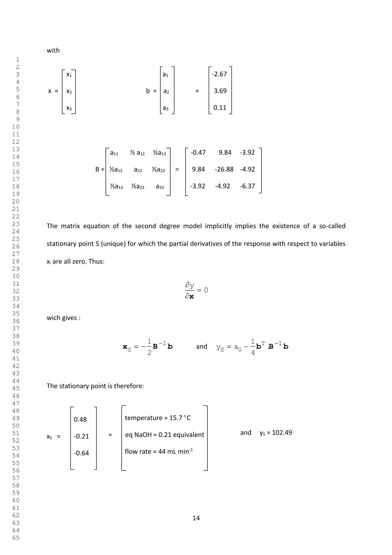
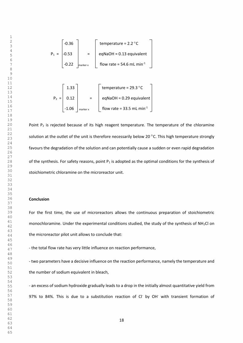

20
Bibliography
(1) Le D M Bougrine A J Pasquet V Delalu H (2019) A new strategy for the synthesis of
monomethylhydrazine using the Raschig process 1 Study of the stability of monochloramine React
Kinet Catal 127(2) 757-773
(2) Ehrfeld W Hessel V Loumlwe H (2000) Microreactors ndash New Technology for Modern Chemistry 1st ed
Wiley VCH Mainz
(3) Hessel V Hardt S Loumlve H (2004) Chemical Micro Process Engineering ndash Fundamentals Modelling
and Reactions Wiley VCH Mainz
(4) Aubin J Xuereb C (2008) Microreacuteacteurs pour lrsquoindustrie Base documentaire Deacuteveloppement de
solvants alternatifs et intensification des proceacutedeacutes Techniques de lrsquoingeacutenieur Ref IN94
(5) Frank T (2008) Microreactors in Organic Synthesis and Catalysis Wiley VCH Weinheim
(6) Goupy J (2001) Introduction aux plans drsquoexpeacuteriences 2nd ed Dunod Paris
(7) Delalu H Duriche C Berthet J Le Gars P (2006) Process for the synthesis of monochloramine US
Patent 7045659
(8) Goupy J (1999) Plans drsquoexpeacuteriences pour surfaces de reacuteponse Dunod Paris
(9) Kamoun A Chaabouni M M Ayedi H F (2011) Plans drsquoexpeacuteriences et traitement de surface ndash
Meacutethodologie des surfaces de reacuteponses Base documentaire Traitements de surface des meacutetaux
contexte et gestion environnementale Technique de lrsquoingeacutenieur Ref M1429
(10) Dodge Y Rousson V (2004) Analyse de reacutegression appliqueacutee Dunod Paris
(11) Brisset S Gillon F Vivier S Brochet P (2001) Optimization with experimental design an approach
using Taguchirsquos methodology and finite element simulations IEEE Transactions on magnetics 37(5)
3530-3533
1 2 3 4 5 6 7 8 9 10 11 12 13 14 15 16 17 18 19 20 21 22 23 24 25 26 27 28 29 30 31 32 33 34 35 36 37 38 39 40 41 42 43 44 45 46 47 48 49 50 51 52 53 54 55 56 57 58 59 60 61 62 63 64 65
21
(12) Lavric E D (2008) Thermal performance of Corning glass microstructures Conference ECI
International Conference on Heat Transfer and Fluid Flow in Microscale Whistler
1 2 3 4 5 6 7 8 9 10 11 12 13 14 15 16 17 18 19 20 21 22 23 24 25 26 27 28 29 30 31 32 33 34 35 36 37 38 39 40 41 42 43 44 45 46 47 48 49 50 51 52 53 54 55 56 57 58 59 60 61 62 63 64 65
22
Table 1 Comparison table of current exchange modules(12)
Module Specific area m2m3
Volumetric thermal transfer coefficient
MWm3sdotK
Batch reactor
25 10-3
Batch reactor with exchanger
10 10-2
Tubular exchanger
400 02
Plate heat exchanger
800 125
Glass Corning microstructure
2500 17
1 2 3 4 5 6 7 8 9 10 11 12 13 14 15 16 17 18 19 20 21 22 23 24 25 26 27 28 29 30 31 32 33 34 35 36 37 38 39 40 41 42 43 44 45 46 47 48 49 50 51 52 53 54 55 56 57 58 59 60 61 62 63 64 65
23
Table 2 Plan 23 experience Matrix summary of the experiments
Experiment number
Factor 1 Factor 2 Factor 3 Answer Temperature Flow rate Pressure NH2Cl Yield ()
1 + + + 869
2 ndash + + 990
3 + ndash + 860
4 + + ndash 926
5 ndash ndash + 995
6 ndash + ndash 990
7 + ndash ndash 832
8 ndash ndash ndash 986
Effective values C mL min-1 bar
Level (+) 30 100 16
Level (ndash) -10 30 7
1 2 3 4 5 6 7 8 9 10 11 12 13 14 15 16 17 18 19 20 21 22 23 24 25 26 27 28 29 30 31 32 33 34 35 36 37 38 39 40 41 42 43 44 45 46 47 48 49 50 51 52 53 54 55 56 57 58 59 60 61 62 63 64 65
24
Table 3 Doehlert plan for three factors summary of experimental tests
Experiment number
Factor 1 Factor 2 Factor 3 Temperature Soda equivalent Flow rate
Encoded value
Real value Encoded
value Real value
Encoded value
Real value
C mL minndash1
1 0 8 0 026 0 60
2 1 24 0 026 0 60
3 05 16 0866 047 0 60
4 -05 0 -0866 005 0 60
5 -1 -8 0 026 0 60
6 -05 0 -0866 005 0 60
7 05 16 -0866 005 0 60
8 0 8 0 026 0 60
9 -05 0 0289 033 0816 80
10 0 8 -0577 012 0816 80
11 05 16 0289 033 0816 80
12 -05 0 -0289 019 -0816 40
13 0 8 0577 040 -0816 40
14 05 16 -0289 019 -0816 40
15 0 8 0 026 0 60
Level ndash1 -8 002 35
Level 0 8 026 60
Level +1 24 050 85
119821 119809 0866 =radic3
2 0816 =
radic2
radic3 0577 =
1
radic3 0289 =
1
2radic3
1 2 3 4 5 6 7 8 9 10 11 12 13 14 15 16 17 18 19 20 21 22 23 24 25 26 27 28 29 30 31 32 33 34 35 36 37 38 39 40 41 42 43 44 45 46 47 48 49 50 51 52 53 54 55 56 57 58 59 60 61 62 63 64 65
25
Table 4 Results of the Doehlert plan experiments
Experiment number
Experimental yield ()
Modelled yield ()
1 9773 9773
2 9996 9940
3 8338 8163
4 8419 8692
5 9556 9612
6 879 8692
7 5462 5462
8 9773 9773
9 8495 8439
10 8532 8357
11 8452 8683
12 9553 9322
13 8292 8467
14 9351 9407
15 9773 9773
1 2 3 4 5 6 7 8 9 10 11 12 13 14 15 16 17 18 19 20 21 22 23 24 25 26 27 28 29 30 31 32 33 34 35 36 37 38 39 40 41 42 43 44 45 46 47 48 49 50 51 52 53 54 55 56 57 58 59 60 61 62 63 64 65
26
Table 5 Fisher test for regression
Source of variation
Degree of liberty
Sum of the squares
Expression Fregression F(095 9 5) Rsup2
Total 15 ndash 1 177370 2
iy -y
59 4772 098 Regression 10 ndash 1 174420 2
iy -y
residual 15 ndash 10 2952 2
i iy -y
1 2 3 4 5 6 7 8 9 10 11 12 13 14 15 16 17 18 19 20 21 22 23 24 25 26 27 28 29 30 31 32 33 34 35 36 37 38 39 40 41 42 43 44 45 46 47 48 49 50 51 52 53 54 55 56 57 58 59 60 61 62 63 64 65
27
Fig 1 Diagram of the Corning microreactor pilot unit
Cooling
system
Cooling
system
Bleach
Sample Release
Release
Waterethanol
1 2 3 4 5 6 7 8 9 10 11 12 13 14 15 16 17 18 19 20 21 22 23 24 25 26 27 28 29 30 31 32 33 34 35 36 37 38 39 40 41 42 43 44 45 46 47 48 49 50 51 52 53 54 55 56 57 58 59 60 61 62 63 64 65
28
Fig 2 Structure created in the MJ microstructure unit to break the flow
mixer Structure created to break the flow
Turbulent flow
MJ microstructure
temperature-
controlled fluid
reagents Product
1 2 3 4 5 6 7 8 9 10 11 12 13 14 15 16 17 18 19 20 21 22 23 24 25 26 27 28 29 30 31 32 33 34 35 36 37 38 39 40 41 42 43 44 45 46 47 48 49 50 51 52 53 54 55 56 57 58 59 60 61 62 63 64 65
29
Fig 3 Coefficients of the mathematical model of the plan 23
-60
-50
-40
-30
-20
-10
00
10
20
30
a1 a2 a3 a12 a13 a23 a123
Co
effi
cien
t va
lue
Temperature
Flow rate
Pressure
1 2 3 4 5 6 7 8 9 10 11 12 13 14 15 16 17 18 19 20 21 22 23 24 25 26 27 28 29 30 31 32 33 34 35 36 37 38 39 40 41 42 43 44 45 46 47 48 49 50 51 52 53 54 55 56 57 58 59 60 61 62 63 64 65
30
Fig 4 Arrangement of Doehlert plan points for 3 factors
Factor 1 Factor 2
Factor 3
Temperature Soda equivalent
Flow rate
1 2 3 4 5 6 7 8 9 10 11 12 13 14 15 16 17 18 19 20 21 22 23 24 25 26 27 28 29 30 31 32 33 34 35 36 37 38 39 40 41 42 43 44 45 46 47 48 49 50 51 52 53 54 55 56 57 58 59 60 61 62 63 64 65
31
Fig 5 Position of the axes during the transformation operations (a) original position (original axes)
(b) positions of the axes during rotation (c) position of the axes during translation
(a) (b) (c)
1 2 3 4 5 6 7 8 9 10 11 12 13 14 15 16 17 18 19 20 21 22 23 24 25 26 27 28 29 30 31 32 33 34 35 36 37 38 39 40 41 42 43 44 45 46 47 48 49 50 51 52 53 54 55 56 57 58 59 60 61 62 63 64 65
32
Fig 6 Variations of the response y according to the axes zi
400
600
800
1000
-1 -075 -05 -025 0 025 05 075 1
value zi
y
z1
z2
z3
1 2 3 4 5 6 7 8 9 10 11 12 13 14 15 16 17 18 19 20 21 22 23 24 25 26 27 28 29 30 31 32 33 34 35 36 37 38 39 40 41 42 43 44 45 46 47 48 49 50 51 52 53 54 55 56 57 58 59 60 61 62 63 64 65
33
Fig 7 Relative positions of the unit vectors of the original and final landmarks (views taken from
different angles)
X1
X1
X1
X1
X2 X2
X2
X2
X3 X3
X3 X3
Z1
Z1
Z1
Z1
Z2
Z2
Z2
Z2
Z3
Z3
Z3
Z3
1 2 3 4 5 6 7 8 9 10 11 12 13 14 15 16 17 18 19 20 21 22 23 24 25 26 27 28 29 30 31 32 33 34 35 36 37 38 39 40 41 42 43 44 45 46 47 48 49 50 51 52 53 54 55 56 57 58 59 60 61 62 63 64 65


![Strategy Synthesis for Linear Arithmetic Gameszkincaid/pub/popl18b.pdf · Strategy Synthesis for Linear Arithmetic Games 61:3 Thomas1995]. Linear reachability games are infinite stateand](https://img.pdfslide.us/doc/110x75/5ec59537e671092f9e18a875/strategy-synthesis-for-linear-arithmetic-games-zkincaidpubpopl18bpdf-strategy.jpg)