Embed Size (px)
Citation preview
ARTICLE IN PRESS
Journal of Economic Dynamics & Control 30 (2006) 1647–1669
0165-1889/$ -
doi:10.1016/j
�CorrespoE-mail ad
www.elsevier.com/locate/jedc
A new statistic and practical guidelines fornonparametric Granger causality testing
Cees Diks�, Valentyn Panchenko
CeNDEF, Department of Economics, University of Amsterdam, Roetersstraat 11,
1018 WB Amsterdam, The Netherlands
Received 4 October 2004; accepted 12 August 2005
Available online 27 April 2006
Abstract
In this paper we introduce a new nonparametric test for Granger non-causality which avoids
the over-rejection observed in the frequently used test proposed by Hiemstra and Jones [1994.
Testing for linear and nonlinear Granger causality in the stock price-volume relation. Journal of
Finance 49, 1639–1664]. After illustrating the problem by showing that rejection probabilities
under the null hypothesis may tend to one as the sample size increases, we study the reason behind
this phenomenon analytically. It turns out that the Hiemstra–Jones test for the null of Granger
non-causality, which can be rephrased in terms of conditional independence of two vectors X and
Z given a third vector Y, is sensitive to variations in the conditional distributions of X and Z that
may be present under the null. To overcome this problem we replace the global test statistic by an
average of local conditional dependence measures. By letting the bandwidth tend to zero at
appropriate rates, the variations in the conditional distributions are accounted for automatically.
Based on asymptotic theory we formulate practical guidelines for choosing the bandwidth
depending on the sample size. We conclude with an application to historical returns and trading
volumes of the Standard and Poor’s index which indicates that the evidence for volume Granger-
causing returns is weaker than suggested by the Hiemstra–Jones test.
r 2006 Elsevier B.V. All rights reserved.
JEL classification: C12; C51; E3
Keywords: Financial time series; Granger causality; Nonparametric; Hypothesis testing; Size distortion;
U-statistics
see front matter r 2006 Elsevier B.V. All rights reserved.
.jedc.2005.08.008
nding author. Tel.: +3120 5255329; fax: +31 20 5254349.
dress: [email protected] (C. Diks).
ARTICLE IN PRESS
C. Diks, V. Panchenko / Journal of Economic Dynamics & Control 30 (2006) 1647–16691648
1. Introduction
Granger (1969) causality has turned out to be a useful notion for characterizingdependence relations between time series in economics and econometrics. Intuitively,for a strictly stationary bivariate process fðX t;Y tÞg, fX tg is a Granger cause of fY tg ifpast and current values of X contain additional information on future values of Y
that is not contained in past and current Y-values alone. If we denote theinformation contained in past observations X s and Y s, spt, by FX ;t and FY ;t,respectively, and let ‘�’ denote equivalence in distribution, the formal definition is:
Definition 1. For a strictly stationary bivariate time series process fðX t;Y tÞg, t 2 Z,fX tg is a Granger cause of fY tg if, for some kX1,
ðY tþ1; . . . ;Y tþkÞjðFX ;t;FY ;tÞfðY tþ1; . . . ;Y tþkÞjFY ;t.
Since this definition is general and does not involve any modelling assumptions, suchas a linear autoregressive model, it is often referred to as general or, by a slight abuseof language, nonlinear Granger causality.
Traditional parametric tests for Granger non-causality within linear autoregres-sive model classes have reached a mature status, and have become part of thestandard toolbox of economists. The recent literature, due to the availability of evercheaper computational power, has shown an increasing interest in nonparametricversions of the Granger non-causality hypothesis against general (linear as well asnonlinear) Granger causality. Among the various nonparametric tests for theGranger non-causality hypothesis, the Hiemstra and Jones (1994) test (hereafter HJtest) is the most frequently used among practitioners in economics and finance.Although alternative tests, such as that proposed by Bell et al. (1996) and by Su andWhite (2003), may also be applied in economics and finance, we limit ourselves to adiscussion of the HJ test and our proposed modification of it.
The reason for considering the HJ test here in detail is our earlier finding (Diksand Panchenko, 2005) that this commonly used test can severely over-reject if thenull hypothesis is true. The aim of the present paper is two-fold. First, we derive theexact conditions under which the HJ test over-rejects, and secondly we propose anew test statistic which does not suffer from this serious limitation. We will showthat the reason for over-rejection of the HJ test is that the test statistic, due to itsglobal nature, ignores the possible variation in conditional distributions that may bepresent under the null hypothesis. Our new test statistic, provided that thebandwidth tends to zero at an appropriate rate, automatically takes into accountsuch variation under the null hypothesis while obtaining an asymptotically correctsize.
The practical implication of our findings is far-reaching: all cases for whichevidence for Granger causality was reported based on the HJ test may be caused bythe tendency of the HJ test to over-reject. Reports of such evidence are numerous inthe economics and finance literature. For instance, Brooks (1998) finds evidence forGranger causality between volume and volatility on the New York Stock Exchange,Abhyankar (1998) and Silvapulla and Moosa (1999) in futures markets, and Ma and
ARTICLE IN PRESS
C. Diks, V. Panchenko / Journal of Economic Dynamics & Control 30 (2006) 1647–1669 1649
Kanas (2000) in exchange rates. Further evidence for causality is reported in stockmarkets (Ciner, 2001), among real estate prices and stock markets (Okunev et al.,2000, 2002) and between London Metal Exchange cash prices and some of itspossible predictors (Chen and Lin, 2004). Although we do not claim that thereported Granger causality is absent in all these cases, we do state that the statisticaljustification is not warranted.
This paper is organized as follows. In Section 2 we show that the HJ test statisticcan give rise to rejection probabilities that tend to one with increasing sample sizeunder the null hypothesis. In Section 3 the reason behind this phenomenon is studiedanalytically and found to be related to a bias in the test statistic due to variations inconditional distributions. The analytic results suggest an alternative test statistic,described in Section 4, which automatically takes these variations into account, andcan be shown to give asymptotic rejection rates equal to the nominal size forbandwidths tending to zero at appropriate rates. The theory is confirmed by thesimulation results presented at the end of the section. In Section 5 we consider anapplication to S&P500 volumes and returns for which the HJ test indicates volumeGranger-causing returns, while our test indicates that the evidence for volumecausing returns is considerably weaker. Section 6 summarizes and concludes.
2. The Hiemstra–Jones test
In testing for Granger non-causality, the aim is to detect evidence against the nullhypothesis
H0 : fX tg is not Granger causing fY tg,
with Granger causality defined according to Definition 1. We limit ourselves to testsfor detecting Granger causality for k ¼ 1, which is the case considered most oftenin practice. Under the null hypothesis Y tþ1 is conditionally independent ofX t;X t�1; . . ., given Y t;Y t�1; . . .. In a nonparametric setting, conditioning on theinfinite past is impossible without a model restriction, such as an assumption that theorder of the process is finite. Therefore, in practice, conditional independence istested using finite lags lX and lY :
Y tþ1jðXlXt ;Y
lYt Þ�Y tþ1jY
lYt ,
where X lXt ¼ ðX t�lXþ1; . . . ;X tÞ and Y lY
t ¼ ðY t�lYþ1; . . . ;Y tÞ. For a strictly stationarybivariate time series fðX t;Y tÞg this is a statement about the invariant distribution ofthe (lX þ lY þ 1)-dimensional vector W t ¼ ðX
lXt ;Y
lYt ;ZtÞ, where Zt ¼ Y tþ1. To keep
the notation compact, and to bring about the fact that the null hypothesis is astatement about the invariant distribution of W t, we often drop the time index andjust write W ¼ ðX ;Y ;ZÞ, where the latter is a random vector with the invariantdistribution of ðX lX
t ;YlYt ;Y tþ1Þ. In this paper we only consider the choice
lX ¼ lY ¼ 1, in which case W ¼ ðX ;Y ;ZÞ denotes a three-variate random variable,distributed as W t ¼ ðX t;Y t;Y tþ1Þ. Throughout we will assume that W is acontinuous random variable.
ARTICLE IN PRESS
C. Diks, V. Panchenko / Journal of Economic Dynamics & Control 30 (2006) 1647–16691650
The HJ test is a modified version of the Baek and Brock (1992) test for conditionalindependence, with critical values based on asymptotic theory. To motivate the teststatistic it is convenient to restate the null hypothesis in terms of ratios of jointdistributions. Under the null the conditional distribution of Z given ðX ;Y Þ ¼ ðx; yÞ isthe same as that of Z given Y ¼ y only, so that the joint probability density functionf X ;Y ;Zðx; y; zÞ and its marginals must satisfy
f X ;Y ;Zðx; y; zÞ
f X ;Y ðx; yÞ¼
f Y ;Zðy; zÞ
f Y ðyÞ, (1a)
or equivalently
f X ;Y ;Zðx; y; zÞ
f Y ðyÞ¼
f X ;Y ðx; yÞ
f Y ðyÞ
f Y ;Zðy; zÞ
f Y ðyÞ(1b)
for each vector ðx; y; zÞ in the support of ðX ;Y ;ZÞ. The last equation is identicalto f X ;ZjY ðx; zjyÞ ¼ f X jY ðxjyÞf ZjY ðzjyÞ, which explicitly states that X and Z areindependent conditionally on Y ¼ y, for each fixed value of y.
The HJ test employs ratios of correlation integrals to measure the discrepancybetween the left- and right-hand sides of (1a). For a multivariate random vector V
taking values in RdV the associated correlation integral CV ðeÞ is the probability offinding two independent realizations of the vector at a distance smaller than or equalto e:
CV ðeÞ ¼ P½kV 1 � V2kpe�; V1;V2 indep. �V
¼
Z ZIðks1 � s2kpeÞf V ðs1Þf V ðs2Þds2 ds1,
where Iðks1 � s2kpeÞ is the indicator function, which is one if ks1 � s2kpe and zerootherwise, and kxk ¼ supi¼1;...;dV
jxij denotes the supremum norm. Hiemstra andJones (1994) argue that (1a) implies for any e40:
CX ;Y ;ZðeÞCX ;Y ðeÞ
¼CY ;ZðeÞCY ðeÞ
(2a)
or equivalently
CX ;Y ;ZðeÞCY ðeÞ
¼CX ;Y ðeÞCY ðeÞ
CY ;ZðeÞCY ðeÞ
. (2b)
The HJ test consists of calculating sample versions of the correlation integrals in(2a), and then testing whether the left-hand- and right-hand-side ratios differsignificantly or not. The estimators for each of the correlation integrals take the form
CW ;nðeÞ ¼2
nðn� 1Þ
XXioj
IWij ,
where IWij ¼ IðkW i �W jkpeÞ. For the asymptotic theory we refer to Hiemstra and
Jones (1994).As stated in the Introduction, the main motivation for the present paper is that in
certain situations the HJ test rejects too often under the null, and we wish to
ARTICLE IN PRESS
C. Diks, V. Panchenko / Journal of Economic Dynamics & Control 30 (2006) 1647–1669 1651
formulate an alternative procedure to avoid this. Before investigating the reasons forover-rejection analytically, we use a simple example to illustrate the over-rejectionnumerically, and to show that simple remedies such as transforming the data touniform marginals and filtering out GARCH structure do not work. Diks andPanchenko (2005) demonstrated that for a process with instantaneous dependencein conditional variance the actual size of the HJ test was severely distorted. Herewe illustrate the same point for a similar process, but without instantaneousdependence:
X t�Nð0; cþ aY 2t�1Þ,
Y t�Nð0; cþ aY 2t�1Þ. ð3Þ
This process satisfies the null hypothesis; fX tg is not Granger causing fY tg. Thevalues for the coefficients a and c are chosen in such a way that the process remainsstationary and ergodic (c40, 0oao1).
We performed some Monte Carlo simulations to obtain the empirical size of theHJ test for the ARCH process (3) with coefficients c ¼ 1, a ¼ 0:4. For varioussample sizes, we generated 1 000 independent realizations of the bivariate processand determined the observed fraction of rejections of the null at a nominal size of0:05.
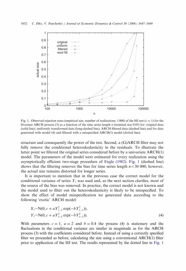
The solid line in Fig. 1 shows the rejection rates found as a function of the timeseries length n. The simulated data were normalized to unit variance before the testwas applied, and the bandwidth was set to e ¼ 1, which is within the common rangeð0:5; 1:5Þ used in practice. For time series length no500 the test based on the originalseries under-rejects. Its size is close to nominal for series length n ¼ 500. For longerseries the actual size increases and becomes close to one when n ¼ 60 000. Thereason that the observed size increases with the series length n is that, as detailed inthe next section, the test statistic is biased in that it does not converge in probabilityto zero under the null as the sample size increases. As the sample size increases thebias converges to a nonzero limit while the variance decreases to zero, giving rise toapparently significant values of the test statistic. In comparison with the process withinstantaneous dependence considered in Diks and Panchenko (2005) the currentprocess indicates less size distortion. This is due to the weaker covariance betweenthe concentration measures HX and HZ for the current process, which is the maincause of the bias.
As suggested by Pompe (1993) in the context of testing for serial independence,transforming the time series to a uniform marginal distribution by using ranks mayimprove the performance of the test. Here we investigate if it reduces the bias of theHJ test. The long-dashed line in Fig. 1 shows that the uniform transform improvesthe size for time series of length n ¼ 1 000, but magnifies the size distortion for timeseries length n42 000.
As another solution one might argue that it is possible to filter out the conditionalheteroskedasticity using a univariate (G)ARCH specification. This would remove thebias caused by the conditional heteroskedasticity in the HJ test. However, such afiltering procedure has several drawbacks. First, it may affect the dependence
ARTICLE IN PRESS
0
0.1
0.2
0.3
0.4
0.5
0.6
0.7
0.8
0.9
1
100 1000 10000 100000
actu
al s
ize
n
originaluniformfilteredexot filt
Fig. 1. Observed rejection rates (empirical size, number of realizations: 1 000) of the HJ test ðe ¼ 1Þ for the
bivariate ARCH process (3) as a function of the time series length n (nominal size 0:05) for: original data(solid line), uniformly transformed data (long-dashed line), ARCH filtered data (dashed line) and for data
generated with model (4) and filtered with a misspecified ARCH(1) model (dotted line).
C. Diks, V. Panchenko / Journal of Economic Dynamics & Control 30 (2006) 1647–16691652
structure and consequently the power of the test. Second, a (G)ARCH filter may notfully remove the conditional heteroskedasticity in the residuals. To illustrate thelatter point we filtered the original series considered before by a univariate ARCH(1)model. The parameters of the model were estimated for every realization using theasymptotically efficient two-stage procedure of Engle (1982). Fig. 1 (dashed line)shows that the filtering removes the bias for time series length no30 000; however,the actual size remains distorted for longer series.
It is important to mention that in the previous case the correct model for theconditional variance of series Y t was used and, as the next section clarifies, most ofthe source of the bias was removed. In practice, the correct model is not known andthe model used to filter out the heteroskedasticity is likely to be misspecified. Toshow the effect of model misspecification we generated data according to thefollowing ‘exotic’ ARCH model:
X t�Nð0; cþ aY 2t�1 expð�bY 2
t�1ÞÞ,
Y t�Nð0; cþ aY 2t�1 expð�bY 2
t�1ÞÞ. ð4Þ
With parameters c ¼ 1, a ¼ 2 and b ¼ 0:4 the process (4) is stationary and thefluctuations in the conditional variance are similar in magnitude as for the ARCHprocess (3) with the coefficients considered before. Instead of using a correctly specifiedfilter we proceeded as before, calculating the size using a conventional ARCH(1) filterprior to application of the HJ test. The results represented by the dotted line in Fig. 1
ARTICLE IN PRESS
C. Diks, V. Panchenko / Journal of Economic Dynamics & Control 30 (2006) 1647–1669 1653
indicate that the misspecified ARCH(1) filter is not able to remove large part of thesource of bias and the sensitivity of the HJ test to dependence in the conditional varianceleads to over-rejection, even for shorter time series.
3. Bias from correlations in conditional concentrations
In this section we show that the reason that the HJ test is inconsistent is that theassumption made by HJ that (1a) implies (2a) does not hold in general. In fact, (2a)follows from (1a) only in specific cases, e.g. when the conditional distributions of Z andX given Y ¼ y do not depend on y. To see this, note that under the null hypothesis
P½kX 1 � X 2koe; kZ1 � Z2koejY 1 ¼ Y 2 ¼ y�
¼ P½kX 1 � X 2koejY 1 ¼ Y 2 ¼ y�P½kZ1 � Z2koejY 1 ¼ Y 2 ¼ y�, ð5Þ
whereas Eq. (2b) states
P½kX 1 � X 2koe; kZ1 � Z2koejkY 1 � Y 2koe�
¼ P½kX 1 � X 2koejkY 1 � Y 2koe�P½kZ1 � Z2koejkY 1 � Y 2koe�. ð6Þ
In general, these conditions are not equivalent. In both equations a statementregarding the factorization of probabilities is made, but the events on which theconditioning takes place differ. In general, under the null the conditionaldistributions of X and Z are allowed to depend on Y. Therefore, the distributionsof X 1 � X 2 and Z1 � Z2 will generally depend, under the null, on Y 1 and Y 2. Forsmall e the condition in Eq. (6) holds for many close but very different Y 1, Y 2 pairs.Therefore, even for small e the left-hand side of Eq. 6 behaves as an average of thatof (5) over all possible values of y. Because factorization of densities is not preservedunder averaging, e.g. af 1ðxÞg1ðzÞ þ ð1� aÞf 2ðxÞf 2ðzÞ typically cannot be written asthe product of a function of x and of z, the average probability on the left-hand sideof (6) will typically not factorize in the form on the right-hand side.
Although this argument shows that the relationship tested in the HJ test isgenerally inconsistent with the null hypothesis, one might argue that the test couldstill be asymptotically valid if appropriate measures are taken to eliminate the ‘bias’in Eq. (2a) asymptotically, for example by allowing for the bandwidth e to tend tozero at an appropriate rate with increasing sample size.
To see whether such an approach might work we examine the behavior of thefractions in (2a) for small values of the bandwidth e. For continuous distributionsthe following small e approximation is useful:
CV ðeÞ ¼Z Z
Iðks1 � s2kpeÞf V ðs1Þf V ðs2Þds1 ds2
¼
Z ZBeðs1Þ
f V ðs2Þds2 f V ðs1Þds1 þ oðedV Þ
¼ ð2eÞdV
Zf 2
V ðsÞdsþ oðedV Þ
¼ ð2eÞdV HV þ oðedV Þ, ð7Þ
ARTICLE IN PRESS
C. Diks, V. Panchenko / Journal of Economic Dynamics & Control 30 (2006) 1647–16691654
where Beðs1Þ denotes a ball (or, since we use the supremum norm, a hypercube) withradius e centred at s1. The constant HV �
Rf 2
V ðsÞds ¼ E½f V ðV Þ� can be consideredas a concentration measure of V. To illustrate this, consider a family of univariatepdfs with scale parameter y, that is, f V ðv; yÞ ¼ y�1gðy�1vÞ for some pdf gð�Þ. Onereadily finds
Rf 2
V ðs; yÞds ¼ ð1=yÞR
g2ðsÞds ¼ cnst:=y, which shows that, in theunivariate case, the concentration measure is inversely proportional to the scaleparameter y. For later convenience, for a pair of vector-valued random variablesðV ;Y Þ of possibly different dimensions, we also introduce the conditional
concentration of the random variable V given Y ¼ y, as HV ðyÞ ¼R
f 2V jY ðvjyÞdv ¼
ðR
f 2V ;Y ðv; yÞdvÞ=f 2
Y ðyÞ.By comparing the leading terms of the expansion in powers of e in Eqs. (2b) and
(7), we find that
E½f X ;Y ;ZðX ;Y ;ZÞ�
E½f Y ðY Þ�¼
E½f X ;Y ðX ;Y Þ�
E½f Y ðY Þ�
E½f Y ;ZðY ;ZÞ�
E½f Y ðY Þ�. (8)
That is, for e small, testing the equivalence of the ratios in (2a) amounts to testing (8)instead of the null hypothesis. Unless some additional conditions hold, this willtypically not be equivalent to testing the null hypothesis. To see what theseadditional conditions are it is useful to rewrite (8) as follows. For the left-hand sideone can write
E½f X ;Y ;ZðX ;Y ;ZÞ�
E½f Y ðY Þ�¼
EY ½EX ;ZjY ½f X ;ZjY ðX ;ZjY Þf ðY Þ��
E½f Y ðY Þ�
¼
ZEX ;ZjY¼y½f X ;ZjY ðX ;ZjyÞ�wðyÞdy
¼
ZHX ;ZðyÞwðyÞdy,
where wðyÞ is a weight function given by wðyÞ ¼ f 2Y ðyÞ=
Rf 2
Y ðsÞds. This brings aboutthe fact that the ratio on the left-hand side of (8) for small e is proportional to aweighted average of the conditional concentration HX ;ZðyÞ, with weight functionwðyÞ. In a similar fashion, for the terms on the right-hand side one derives
E½f X ;Y ðX ;Y Þ�
E½f Y ðY Þ�¼
ZHX ðyÞwðyÞdy and
E½f Y ;ZðY ;ZÞ�
E½f Y ðY Þ�¼
ZHZðyÞwðyÞdy.
Under the null hypothesis, Z is conditionally independent of X given Y ¼ y,so that HX ;ZðyÞ is equal to HX ðyÞHZðyÞ, for all y. It follows that the left- and right-hand sides of (8) coincide under the null if and only if
RHX ðyÞHZðyÞwðyÞdy�R
HX ðyÞwðyÞdyR
HZðyÞwðyÞdy ¼ 0, or
CovðHX ðSÞ;HZðSÞÞ ¼ 0, (9)
where S is a random variable with pdf wðyÞ. Only under specific conditions, such aseither HX ðyÞ or HZðyÞ being independent of y, (9) holds under the null, and hence(2a) as e tends to zero. Also if HX ðyÞ and HZðyÞ depend on y, (9) may hold, but this isan exception rather than the rule. Typically the covariance between the conditional
ARTICLE IN PRESS
C. Diks, V. Panchenko / Journal of Economic Dynamics & Control 30 (2006) 1647–1669 1655
concentrations of X and Z given Y will not vanish, inducing a bias in the HJ test forsmall e.
Therefore, letting the bandwidth tend to zero with increasing sample size in the HJtest would not provide a theoretical solution to the problem of over- or under-rejection caused by positive or negative covariance of the concentration measures,respectively. In simulations for a particular process and small to moderate samplesizes one can often identify a seemingly adequate rate for bandwidths vanishingaccording to en ¼ Cn�b, for which the size of the HJ test remains close to nominal.However, this does not imply that using the HJ test with such a sample sizedependent bandwidth is advisable in practice. The optimal choices for C and b maydepend strongly on the data generating process, and our results show thatasymptotically the HJ test for typical processes (those with non-vanishing covarianceof concentrations of X and Y) is inconsistent.
The fact that the conditional concentration measures of X lXt and Y tþ1 given Y lY
t
affect the leading bias term poses severe restrictions on applicability to economic andfinancial time series in which conditional heteroskedasticity is usually present.Consequently, there is a risk of over-rejection by the HJ test which cannot be easilyeliminated either by using (G)ARCH filtering, or by using a bandwidth thatdecreases with the sample size. To avoid this problem, in the next section we suggesta new test statistic for which a consistent test is obtained as e tends to zero at theappropriate rate. The idea is to measure the dependence between X and Z givenY ¼ yi locally for each yi. By allowing for the bandwidth to decrease with the samplesize, variations in the local (fixed Y) conditional distributions of X and Z given Y areautomatically taken into account by the test statistic.
4. A modified test statistic
In comparing Eqs. (1b) and (8) it can be noticed that although (1b) holds point-wise for any triple ðx; y; zÞ in the support of f X ;Y ;Zðx; y; zÞ, (8) contains separateaverages for the nominator and the denominator of (1b), which do not respect thefact that the y-values on the rhs of (1b) should be identical. Eq. (1b) holds point-wise.Therefore, rather than (8), the null hypothesis implies
qg � Ef X ;Y ;ZðX ;Y ;ZÞ
f Y ðY Þ�
f X ;Y ðX ;Y Þ
f Y ðY Þ
f Y ;ZðY ;ZÞ
f Y ðY Þ
� �gðX ;Y ;ZÞ
� �¼ 0,
where gðx; y; zÞ is a positive weight function. Under the null hypothesis the termwithin the round brackets vanishes, so that the expectation is zero. Although qg isnot positive definite, a one-sided test, rejecting when its estimated value is too large,in practice is often found to have larger power than a two-sided test. In tests forserial dependence Skaug and Tjøstheim (1993) report good performance of a closelyrelated unconditional test statistic (their dependence measure I4 is an unconditionalversion of our term in round brackets).
We have considered several possible choices of the weight function g, being(i) g1ðx; y; zÞ ¼ f Y ðyÞ, (ii) g2ðx; y; zÞ ¼ f 2
Y ðyÞ and (iii) g3ðx; y; zÞ ¼ f Y ðyÞ=f X ;Y ðx; yÞ.
ARTICLE IN PRESS
C. Diks, V. Panchenko / Journal of Economic Dynamics & Control 30 (2006) 1647–16691656
Monte Carlo simulations using the stationary bootstrap (Politis and Romano, 1994)indicated that g1 and g2 behave similarly and are more stable than g3. We will focus ong2 in this paper, as its main advantage over g1 is that the corresponding estimator hasa representation as a U-statistic, allowing the asymptotic distribution to be derivedanalytically for weakly dependent data, thus eliminating the need of a computationallymore requiring bootstrap procedure. For the choice gðx; y; zÞ ¼ f 2
Y ðyÞ, we refer to thecorresponding functional simply as q:
q ¼ E½f X ;Y ;ZðX ;Y ;ZÞf Y ðY Þ � f X ;Y ðX ;Y Þf Y ;ZðY ;ZÞ�.
A natural estimator of q based on indicator functions is
TnðeÞ ¼ð2eÞ�dX�2dY�dZ
nðn� 1Þðn� 2Þ
Xi
Xk;kai
Xj;jai
ðIXYZik IY
ij � IXYik IYZ
ij Þ
" #,
where IWij ¼ IðkW i �W jkoeÞ. Note that the terms with k ¼ j need not be excluded
explicitly as these each contribute zero to the test statistic. The test statistic can beinterpreted as an average over local BDS test statistics (see Brock et al., 1996), for theconditional distribution of X and Z, given Y ¼ yi.
If we denote local density estimators of a dW -variate random vector W at W i by
bf W ðW iÞ ¼ð2eÞ�dW
n� 1
Xj;jai
IWij ,
the test statistic simplifies to
TnðeÞ ¼ðn� 1Þ
nðn� 2Þ
Xi
ðbf X ;Y ;ZðX i;Y i;ZiÞbf Y ðY iÞ �
bf X ;Y ðX i;Y iÞbf Y ;ZðY i;ZiÞÞ.
For an appropriate sequence en of bandwidth values these estimators are consistentand the test statistic consist of a weighted average of local contributionsbf X ;Y ;Zðx; y; zÞbf Y ðyÞ �
bf X ;Y ðx; yÞbf Y ;Zðy; zÞ which tend to zero in probability underthe null hypothesis.
In A.1, using the approach proposed by Powell and Stoker (1996), we show thatfor dX ¼ dY ¼ dZ ¼ 1 the test is consistent if we let the bandwidth depend on thesample size as
en ¼ Cn�b (10)
for any positive constant C and b 2 ð14; 13Þ. In that case the test statistic is
asymptotically normally distributed in the absence of dependence between thevectors W i. Under suitable mixing conditions (Denker and Keller, 1983) this can beextended to a time series context provided that covariances between the local densityestimators are taken into account, giving:
Theorem 1. For a sequence of bandwidths en given by (10) with C40 and b 2 ð14; 13Þ the
test statistic Tn satisfiesffiffiffinp ðTnðenÞ � qÞ
Sn
�!d
Nð0; 1Þ.
ARTICLE IN PRESS
C. Diks, V. Panchenko / Journal of Economic Dynamics & Control 30 (2006) 1647–1669 1657
In A.1 the asymptotic normality of Tn is shown under a decreasing bandwidth,while A.3 considers the autocorrelation robust estimation of the asymptotic variances2 by S2
n.
4.1. Bandwidth choice
In the typical case where the local bias tends to zero at the rate e2 as in Condition 1in A.1, the bandwidth choice which is optimal in that it asymptotically gives theestimator Tn with the smallest mean squared error (MSE) is given by
e�n ¼ C�n�2=7
with
C� ¼18 � 3q2
4ðE½sðW Þ�Þ2
� �1=7
(11)
as derived in Appendix A.2.To gain some insights into the order of magnitude of C� it is helpful to calculate its
value for some processes. Here we consider the ARCH process given in (3). Theoptimal C-value derived in the appendix is analytically hard to track since it involvesthe marginal distribution of the process. However, we can derive an approximateoptimal value of C analytically by ignoring the deviation from normality of Y (anassumption which is reasonable for small a). Taking Y�Nð0; 1Þ and X ;Z independentand Nð0; 1þ aY 2Þ conditional on Y, we find
q2 ¼e2=aerfcð
ffiffiffiffiffiffiffiffi2=a
pÞ
1152p2ffiffiffiap , (12)
where erfcðsÞ ¼ 1� erfðsÞ and
E½sðW Þ� ¼
ffiffiffiffiffiffiffiffiffiffi6a=p
pð3þ aÞ þ ðaða� 6Þ � 9Þe3=ð2aÞerfcð
ffiffiffiffiffiffiffiffiffiffiffiffiffi3=ð2aÞ
pÞ
768ffiffiffi2p
a3=2p3=2. (13)
To investigate the behaviour of the bandwidth for small a, one may use the factthat
q2 ¼1
1152ffiffiffi2p
p3=2þ oðaÞ and E½sðW Þ� ¼ a2 1
288ffiffiffi3p
p2þ oðaÞ
� �.
This suggests that as a tends to zero the (asymptotically) optimal bandwidth divergesat the rate a�4=7. This is consistent with the fact that larger bandwidths are optimalfor a smaller correlation between the conditional concentrations of X and Z given Y.
The optimal bandwidth for (G)ARCH filtered data depends on the correlation ofthe conditional concentrations of X and Z given Y after filtering, which may dependstrongly on the underlying data generating process. However, the consistency of thetest does not require filtering prior to testing, and it is possible to obtain a roughindication of the optimal bandwidth for raw returns. Since the covariance betweenconditional concentrations for bivariate financial time series are mainly due to
ARTICLE IN PRESS
C. Diks, V. Panchenko / Journal of Economic Dynamics & Control 30 (2006) 1647–16691658
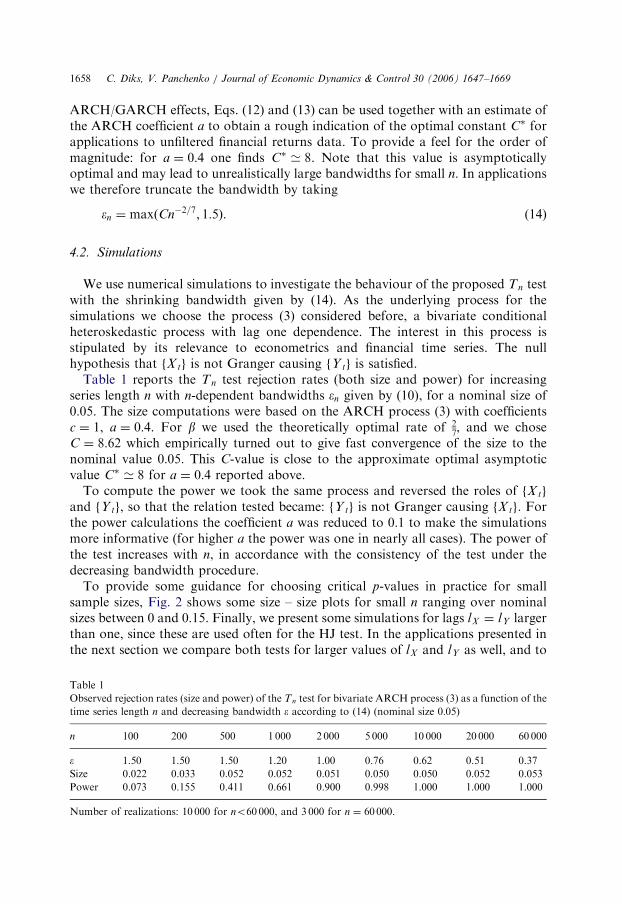
ARCH/GARCH effects, Eqs. (12) and (13) can be used together with an estimate ofthe ARCH coefficient a to obtain a rough indication of the optimal constant C� forapplications to unfiltered financial returns data. To provide a feel for the order ofmagnitude: for a ¼ 0:4 one finds C� ’ 8. Note that this value is asymptoticallyoptimal and may lead to unrealistically large bandwidths for small n. In applicationswe therefore truncate the bandwidth by taking
en ¼ maxðCn�2=7; 1:5Þ. (14)
4.2. Simulations
We use numerical simulations to investigate the behaviour of the proposed Tn testwith the shrinking bandwidth given by (14). As the underlying process for thesimulations we choose the process (3) considered before, a bivariate conditionalheteroskedastic process with lag one dependence. The interest in this process isstipulated by its relevance to econometrics and financial time series. The nullhypothesis that fX tg is not Granger causing fY tg is satisfied.
Table 1 reports the Tn test rejection rates (both size and power) for increasingseries length n with n-dependent bandwidths en given by (10), for a nominal size of0:05. The size computations were based on the ARCH process (3) with coefficientsc ¼ 1, a ¼ 0:4. For b we used the theoretically optimal rate of 2
7, and we chose
C ¼ 8:62 which empirically turned out to give fast convergence of the size to thenominal value 0:05. This C-value is close to the approximate optimal asymptoticvalue C� ’ 8 for a ¼ 0:4 reported above.
To compute the power we took the same process and reversed the roles of fX tg
and fY tg, so that the relation tested became: fY tg is not Granger causing fX tg. Forthe power calculations the coefficient a was reduced to 0:1 to make the simulationsmore informative (for higher a the power was one in nearly all cases). The power ofthe test increases with n, in accordance with the consistency of the test under thedecreasing bandwidth procedure.
To provide some guidance for choosing critical p-values in practice for smallsample sizes, Fig. 2 shows some size – size plots for small n ranging over nominalsizes between 0 and 0:15. Finally, we present some simulations for lags lX ¼ lY largerthan one, since these are used often for the HJ test. In the applications presented inthe next section we compare both tests for larger values of lX and lY as well, and to
Table 1
Observed rejection rates (size and power) of the Tn test for bivariate ARCH process (3) as a function of the
time series length n and decreasing bandwidth e according to (14) (nominal size 0:05)
n 100 200 500 1 000 2 000 5 000 10 000 20 000 60 000
e 1.50 1.50 1.50 1.20 1.00 0.76 0.62 0.51 0.37
Size 0.022 0.033 0.052 0.052 0.051 0.050 0.050 0.052 0.053
Power 0.073 0.155 0.411 0.661 0.900 0.998 1.000 1.000 1.000
Number of realizations: 10 000 for no60 000, and 3 000 for n ¼ 60 000.

ARTICLE IN PRESS
0
0.025
0.05
0.075
0.1
0.125
0.15
0 0.025 0.05 0.075 0.1 0.125 0.15
actu
al s
ize
nominal size
n=100n=200n=500
Fig. 2. Size – size plot of Tn test for process (3) with shrinking bandwidth for time series lengths n ¼ 100
(solid line), 200 (dashed line), 500 (long-dashed line). The number of realizations is 10 000. The dotted line
along the diagonal represents the ideal situation where the actual size and the nominal size coincide.
C. Diks, V. Panchenko / Journal of Economic Dynamics & Control 30 (2006) 1647–1669 1659
motivate this we should check if the empirical size of our new test does not exceed thenominal size for larger lags.
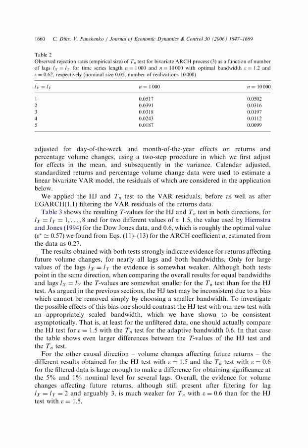
Table 2 gives the empirical rejection rates for the bivariate ARCH process (3),again with c ¼ 1 and a ¼ 0:4, under the null hypothesis (that is, testing fX tg Grangercauses fY tg) for lag lengths lX ¼ lY ranging from 1 to 5. The results indicate that therejection rate decreases with lX ¼ lY , and hence that the Tn test is progressivelyconservative for increasing lag lengths, so that the risk of rejecting under the nullbecomes small.
5. Applications
We consider an application to daily volume and returns data for the Standard andPoor’s 500 index in the period between January 1950 and December 1990. We havedeliberately chosen this period to roughly correspond to the period for whichHiemstra and Jones (1994) found strong evidence for volume Granger-causingreturns (1947–1990) for the Dow Jones index. To keep our results comparable withthose of Hiemstra and Jones, we closely followed their procedure. That is, we
ARTICLE IN PRESS
Table 2
Observed rejection rates (empirical size) of Tn test for bivariate ARCH process (3) as a function of number
of lags lX ¼ lY for time series length n ¼ 1 000 and n ¼ 10 000 with optimal bandwidth e ¼ 1:2 and
e ¼ 0:62, respectively (nominal size 0.05, number of realizations 10 000)
lX ¼ lY n ¼ 1 000 n ¼ 10 000
1 0.0517 0.0502
2 0.0391 0.0316
3 0.0318 0.0197
4 0.0243 0.0112
5 0.0187 0.0099
C. Diks, V. Panchenko / Journal of Economic Dynamics & Control 30 (2006) 1647–16691660
adjusted for day-of-the-week and month-of-the-year effects on returns andpercentage volume changes, using a two-step procedure in which we first adjustfor effects in the mean, and subsequently in the variance. Calendar adjusted,standardized returns and percentage volume change data were used to estimate alinear bivariate VAR model, the residuals of which are considered in the applicationbelow.
We applied the HJ and Tn test to the VAR residuals, before as well as afterEGARCH(1,1) filtering the VAR residuals of the returns data.
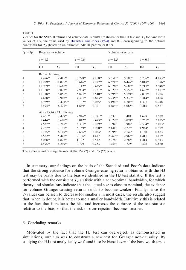
Table 3 shows the resulting T-values for the HJ and Tn test in both directions, forlX ¼ lY ¼ 1; . . . ; 8 and for two different values of e: 1:5, the value used by Hiemstraand Jones (1994) for the Dow Jones data, and 0:6, which is roughly the optimal value(e� ’ 0:57) we found from Eqs. (11)–(13) for the ARCH coefficient a, estimated fromthe data as 0:27.
The results obtained with both tests strongly indicate evidence for returns affectingfuture volume changes, for nearly all lags and both bandwidths. Only for largevalues of the lags lX ¼ lY the evidence is somewhat weaker. Although both testspoint in the same direction, when comparing the overall results for equal bandwidthsand lags lX ¼ lY the T-values are somewhat smaller for the Tn test than for the HJtest. As argued in the previous sections, the HJ test may be inconsistent due to a biaswhich cannot be removed simply by choosing a smaller bandwidth. To investigatethe possible effects of this bias one should contrast the HJ test with our new test withan appropriately scaled bandwidth, which we have shown to be consistentasymptotically. That is, at least for the unfiltered data, one should actually comparethe HJ test for e ¼ 1:5 with the Tn test for the adaptive bandwidth 0:6. In that casethe table shows even larger differences between the T-values of the HJ test andthe Tn test.
For the other causal direction – volume changes affecting future returns – thedifferent results obtained for the HJ test with e ¼ 1:5 and the Tn test with e ¼ 0:6for the filtered data is large enough to make a difference for obtaining significance atthe 5% and 1% nominal level for several lags. Overall, the evidence for volumechanges affecting future returns, although still present after filtering for laglX ¼ lY ¼ 2 and arguably 3, is much weaker for Tn with e ¼ 0:6 than for the HJtest with e ¼ 1:5.
ARTICLE IN PRESS
Table 3
T-ratios for the S&P500 returns and volume data. Results are shown for the HJ test and Tn for bandwidth
values of 1:5, the value used by Hiemstra and Jones (1994) and 0:6, corresponding to the optimal
bandwidth for Tn (based on an estimated ARCH parameter 0:27)
lX ¼ lY Returns) volume Volume) returns
e ¼ 1:5 e ¼ 0:6 e ¼ 1:5 e ¼ 0:6
HJ T2 HJ T2 HJ T2 HJ T2
Before filtering
1 9.476�� 9.415�� 10.298�� 8.850�� 5.351�� 5.106�� 5.736�� 4.893��
2 10.989�� 11.076�� 10.616�� 8.182�� 6.671�� 6.447�� 6.818�� 5.396��
3 10.909�� 10.662�� 9.112�� 6.425�� 6.026�� 5.683�� 5.717�� 3.948��
4 10.758�� 9.823�� 7.934�� 5.121�� 6.029�� 5.552�� 4.692�� 2.887��
5 10.118�� 8.856�� 5.821�� 3.540�� 5.695�� 5.191�� 2.837�� 1.234
6 9.428�� 7.903�� 4.391�� 2.603�� 5.935�� 5.338�� 3.314�� 1.604
7 8.959�� 7.4215�� 3.102�� 2.085� 5.194�� 4.706�� 1.327 0.248
8 8.494�� 6.577�� 1.649� 0.701 4.484�� 4.085�� 0.418 0.567
After EGARCH filtering
1 7.461�� 7.429�� 7.946�� 6.781�� 1.532 1.481 1.628 1.529
2 8.444�� 8.600�� 8.012�� 6.493�� 3.022�� 3.091�� 3.251�� 2.825��
3 7.537�� 7.788�� 6.381�� 5.109�� 1.894� 1.982� 2.534�� 2.023�
4 7.257�� 7.198�� 5.169�� 3.900�� 2.141� 2.225� 1.964� 0.989
5 6.125�� 6.107�� 2.686�� 2.023� 2.095� 2.142� 1.160 0.853
6 5.582�� 5.445�� 2.136� 1.477 2.969�� 2.965�� 1.411 1.129
7 5.028�� 4.873�� 1.192 0.532 2.278� 2.285� 1.414 0.943
8 4.495�� 4.249�� 0.779 0.253 1.754� 1.725� 0.398 0.860
The asterisks indicate significance at the 5% (*) and 1% (**) levels.
C. Diks, V. Panchenko / Journal of Economic Dynamics & Control 30 (2006) 1647–1669 1661
In summary, our findings on the basis of the Standard and Poor’s data indicatethat the strong evidence for volume Granger-causing returns obtained with the HJtest may be partly due to the bias we identified in the HJ test statistic. If the test isperformed with the consistent Tn statistic with a near-optimal bandwidth, for whichtheory and simulations indicate that the actual size is close to nominal, the evidencefor volume Granger-causing returns tends to become weaker. Finally, since theT-values can be seen to decrease for smaller e in most cases, the results also suggestthat, when in doubt, it is better to use a smaller bandwidth. Intuitively this is relatedto the fact that it reduces the bias and increases the variance of the test statisticrelative to the bias, so that the risk of over-rejection becomes smaller.
6. Concluding remarks
Motivated by the fact that the HJ test can over-reject, as demonstrated insimulations, our aim was to construct a new test for Granger non-causality. Bystudying the HJ test analytically we found it to be biased even if the bandwidth tends
ARTICLE IN PRESS
C. Diks, V. Panchenko / Journal of Economic Dynamics & Control 30 (2006) 1647–16691662
to zero. Based on the analytic results, which indicated that the bias is caused bycovariances in conditional concentrations, we proposed a new test statistic Tn thatautomatically takes the variation in concentrations into account.
By symmetrizing the new test statistic, we expressed it as a U-statistic for which wedeveloped asymptotic theory under bandwidth values that tend to zero with thesample size at appropriate rates. The theory allowed us to derive the optimal rate aswell as the asymptotically optimal multiplicative factor for the bandwidth. ForARCH type processes the optimal bandwidth can be expressed in terms of theARCH coefficient, which is useful for getting an indication of the order of magnitudeof the bandwidth to be used in practice for financial returns data. Simulations for thenew test confirmed that the size converges to the nominal size fast as the sample sizeincreases. Additional simulations indicated that the test becomes conservative forlarger lags taken into account by the test.
In an application to relative volume changes and returns for historic Standard andPoor’s index data we found that some of the strong evidence for relative volumechanges Granger-causing returns obtained with the HJ test may be related to its bias,since use of the new test, which is shown to be consistent, strongly weakens theevidence against the null hypothesis. This result suggests that some of the rejectionsof the Granger non-causality hypothesis reported in the literature may be spurious.
Appendix A
A.1. Asymptotic distribution of Tn
The test statistic Tn can be written in terms of a U-statistic by symmetrization withrespect to the three different indices. This gives
TnðeÞ ¼1
nðn� 1Þðn� 2Þ
Xiajakai
KðW i;W j ;W kÞ
with W i ¼ ðXlX
i ;YlY
i ;ZiÞ, i ¼ 1; . . . ; n, and
KðW i;W j ;W kÞ ¼ð2eÞ�dX�2dY�dZ
6
ðIXYZik IY
ij � IXYik IYZ
ij Þ þ ðIXYZij IY
ik � IXYij IYZ
ik Þþ
ðIXYZjk IY
ji � IXYjk IYZ
ji Þ þ ðIXYZji IY
jk � IXYji IYZ
jk Þþ
ðIXYZki IY
kj � IXYki IYZ
kj Þ þ ðIXYZkj IY
ki � IXYkj IYZ
ki Þ
0BB@1CCA.
For a given bandwidth e the test statistic Tn is a third order U-statistic. To developasymptotic distribution theory under a shrinking bandwidth en we closely follow themethodology proposed by Powell and Stoker (1996). Although their main goal wasto derive MSE (mean squared error) optimal bandwidths for point estimators, itturns out that similar considerations can be used to derive rates for the bandwidththat provide consistency and asymptotic normality of Tn. We first treat theanalytically simplest case of a random sample fW ig
ni¼1, and deal with dependence
later.
ARTICLE IN PRESS
C. Diks, V. Panchenko / Journal of Economic Dynamics & Control 30 (2006) 1647–1669 1663
Because Tn is a U-statistic, its finite sample variance is given by (see e.g. Serfling,1980)
VarðTnÞ ¼9
nz1 þ
18
n2z2 þ
6
n3z3 þ o
z1nþ
z2n2þ
z3n3
� �,
where
z1 ¼ CovðKðW 1;W 2;W 3Þ;KðW 1;W02;W
03ÞÞ ¼ VarðK1ðW 1ÞÞ,
z2 ¼ CovðKðW 1;W 2;W 3Þ;KðW 1;W 2;W03Þ ¼ VarðK2ðW 1;W 2ÞÞ,
z3 ¼ VarðKðW 1;W 2;W 3ÞÞ,
with W 1;W 2;W 3;W02 and W 0
3 all independent and identically distributed accordingto W . The functions K1ðw1Þ and K2ðw1;w2Þ are given by K1ðw1Þ ¼ E½Kðw1;W 2;W 3Þ�
and K2ðw1;w2Þ ¼ E½Kðw1;w2;W 3Þ�.Following Powell and Stoker (1996), define rðw; eÞ ¼ K1ðw; eÞ and r0ðwÞ ¼
lime!0rðw; eÞ. It can be verified that
r0ðwÞ ¼2
3f X ;Y ;Zðx; y; zÞ f Y ðyÞ þ
1
3f 2
Y ðyÞHX ;ZðyÞ �1
3f X ;Y ðx; yÞ f Y ;Zðy; zÞ
�1
3f Y ;Zðy; zÞ f Y ðyÞ
Zf X ;Y ðx
0; yÞ f X ;Y ;Zðx0; y; zÞdx0
�1
3f X ;Y ðx; yÞ f Y ðyÞ
Zf Y ;Zðy; z
0Þ f X ;Y ;Zðx; y; z0Þdz0.
For example, the fourth term on the right-hand side follows from
ð2eÞ�dX�2dY�dZEW k½IXY
jk IYZji �
¼
Zf X ;Y ðxk; ykÞdxj ;yj
ðxk; ykÞIYZij dxk dykð2eÞ
�dY�dZ þ oð1Þ
¼ f X ;Y ðxj ; yjÞIYZij ð2eÞ
�dY�dZ þ oð1Þ,
where dv0 ðvÞ stands for the Kronecker delta function, which can be thought of as thelimiting pdf of a random variable with all mass at the point v0, and
ð2eÞ�dY�dZEW j½ f X ;Y ðxj ; yjÞI
YZij �
¼
Zf X ;Y ðxj ; yjÞdyj ;zj
ðyi; ziÞ f X ;Y ;Zðxj ; yj ; zjÞdxj dyj dzj þ oð1Þ
¼
Zf X ;Y ðxj ; yiÞ f X ;Y ;Zðxj ; yi; ziÞdxj þ oð1Þ.
Adapting from Powell and Stoker (1996), we assume the following threeconditions:
Condition 1 (Rate of convergence of pointwise bias of rðwi; eÞ). The functions rðwi; eÞsatisfy
rðwi; eÞ � r0ðwiÞ ¼ sðwiÞea þ s�ðwi; eÞ,
for some a40, and the remainder term s�ð�Þ satisfies Eks�ðW i; hÞk2 ¼ oðh2a
Þ.
ARTICLE IN PRESS
C. Diks, V. Panchenko / Journal of Economic Dynamics & Control 30 (2006) 1647–16691664
For our kernel the bias in each of the contributions to the kernel converges to zeroat rate a ¼ 2. Therefore Condition 1 holds with a ¼ 2. In fact, it might be possible toreplace the local bias Condition 1 by a global version, involving E½rðW i; eÞ � r0ðW iÞ�,which may tend to zero faster than the local bias. However, for our purposes thelocal assumption with a ¼ 2 suffices.
Condition 2 (Series expansion for second moment of K2ðW 1;W 2Þ). The function
K2ðw1;w2Þ satisfies
E½ðK2ðW 1;W 2ÞÞ2� ¼ q2e
�g þ q�2ðeÞ
for some g40, where the remainder term q�2 satisfies ðq�2ðeÞÞ2¼ oðe�gÞ.
This is a weaker version of Powell and Stoker’s (1996) Assumption 2, whichrequired a series expansion locally. For our purposes the weaker assumption suffices,since Tn is a global functional of the distribution of W .
Condition 3 (Series expansion for second moment of KðW 1;W 2;W 3Þ). The function
Kðw1;w2;w3Þ satisfies
E½ðKðW 1;W 2;W 3ÞÞ2� ¼ q3e
�d þ q�3ðeÞ
for some d40, where the remainder term q�3 satisfies ðq�3ðeÞÞ2¼ oðe�dÞ.
For our kernel Condition 3 is satisfied with d ¼ dX þ 2dY þ dZ, since none of thecontributions to the kernel have a variance increasing faster in e than at the rateedXþ2dYþdZ . Finding an appropriate value for g in Condition 2 is somewhat moreinvolved. We examine the rate at which each of the contributions to the kernelfunction depend on e. For example, for the term ð2eÞ�dX�2dY�dZ IXYZ
ik IYij we find
EW k½ð2eÞ�dX�2dY�dZ IXYZ
ik IYij � ¼ ð2eÞ
�dY f X ;Y ;ZðX i;Y i;ZiÞIYij þ oð1Þ from which one
obtains
E½ðð2eÞ�dY EW k½IXYZ
ik IYij �Þ
2� ¼ ð2eÞ�2dYE½ f 2
X ;Y ;ZðX i;Y i;ZiÞIYij þ oðedY Þ�
¼ ð2eÞ�dY E½ f 2X ;Y ;ZðX i;Y i;ZiÞ f Y ðY iÞ� þ oðe�dY Þ.
Proceeding in this way for each of the terms in the kernel, one finds that the dominant
contributions are given by the terms ð2eÞ�dX�2dY�dZ IXYZij IY
ik and ð2eÞ�dX�2dY�dZ IXYZji IY
jk .
For the first of these one finds EW k½ð2eÞ�dX�2dY�dZ IXYZ
ij IYik � ¼ ð2eÞ
�dX�dY�dZ IXYZij
f Y ðY iÞ þ oð1Þ, giving
E½ðð2eÞ�dX�dY�dZEW k½IXYZ
ij IYik�Þ
2�
¼ ð2eÞ�2dX�2dY�2dZE½IXYZij f 2
Y ðY iÞ� þ oðe�dX�dY�dZ Þ
¼ ð2eÞ�dX�dY�dZE½ f X ;Y ;ZðX i;Y i;ZiÞ f2Y ðY iÞ� þ oðe�dX�dY�dZ Þ.
All other terms increase with vanishing e slower, which demonstrates that Condition
2 holds with g ¼ dX þ dY þ dZ and a constant q2 given by q2 ¼436� 2�dX�dY�dZ
E½ f X ;Y ;ZðX i;Y i;ZiÞ f2Y ðY iÞ�. The factor 4 enters due to the fact that there are
ARTICLE IN PRESS
C. Diks, V. Panchenko / Journal of Economic Dynamics & Control 30 (2006) 1647–1669 1665
two terms, EW k½ð2eÞ�dX�2dY�dZ IXYZ
ij IYik� and EW k
½ð2eÞ�dX�2dY�dZ IXYZij IY
jk�, which are
asymptotically perfectly correlated if e tends to zero sufficiently slowly with thesample size.
It follows from Condition 1 that
Var½rðW i; eÞ� ¼ Var½r0ðW iÞ� þ C0ea þ oðeaÞ,
where C0 ¼ 2Cov½r0ðW iÞ; sðW iÞ�. We can thus express the mean squared errorof Tn as
MSE½Tn� ¼ ðE½sðW iÞ�Þ2e2a þ
9
nC0ea þ
9
nVar½r0ðW iÞ� þ
18
n2q2e�g þ
6
n3q3e�d.
(15)
Tn is asymptotically Nð0;s2=nÞ distributed with s2 ¼ 9Var½r0ðW iÞ�, provided thateach of the e-dependent terms in the MSE of Tn are oðn�1Þ. If we let e�n�b, thisimplies the following four conditions hold:
�2abo� 1; �abo0; gbo1; dbo2.
The first two of these imply b41=2a ¼ 14and b40, respectively, while the last
two imply bo1=g ¼ 1=ðdX þ dY þ dZÞ and bo2=d ¼ 2=ðdX þ 2dY þ dZÞ. Because1=ðdX þ dY þ dZÞo2=ðdX þ 2dY þ dZÞ, the conditions can be summarized as:14obo1=ðdX þ dY þ dZÞ. Therefore, for the case dX ¼ dY ¼ dZ ¼ 1, and a sequenceof bandwidths en�n�b for some b 2 ð1
4; 13Þ, the test statistic is asymptotically normal:ffiffiffi
np TnðenÞ � q
s�!d
Nð0; 1Þ
with s2 ¼ 9Var½r0ðW iÞ�.Note that it might also be possible to derive appropriate values for the rate b for
dX þ dY þ dZ43, but only provided that the overall bias E½sðW iÞ� tends to zerofaster than e2.
A.2. Optimal bandwidth
The MSE optimal bandwidth balances the dominating squared bias and varianceterms (the first and fourth terms on the right-hand side of Eq. (15)), the otherbandwidth dependent terms being of smaller order. The optimal bandwidth whichasymptotically minimizes the sum of these terms is given by
e� ¼18 � 3q2
4ðE½sðW Þ�Þ2
� �1=7
n�2=7. (16)
To guide the choice of the multiplicative factor C in e ¼ Cn�2=7, it is illustrative toexamine the optimal choice C� ¼ 18 � 3q2=4ðE½sðW Þ�Þ
2� �1=7
in specific cases. Abovean expression for q2 was found already in terms of the joint density of W . A similarexpression for E½sðW iÞ� can be found by using local Taylor expansions of the densityof w, locally near wk. As each of the six terms in Tn have the same expectation,
ARTICLE IN PRESS
C. Diks, V. Panchenko / Journal of Economic Dynamics & Control 30 (2006) 1647–16691666
to determine the bias we consider the first of these only:
ð2eÞ�dX�2dY�dZ ðIXYZik IY
ij � IXYik IYZ
ij Þ.
Taking averages over j and k for a fixed vector wi leads to an expression involvingplug-in estimators of local densities
ð2eÞ�dX�2dY�dZ
ðn� 1Þðn� 2Þ
Xjai
Xkai; j
ðIXYZik IY
ij � IXYik IYZ
ij Þ
¼ bf X ;Y ;Zðxi; yi; ziÞbf Y ðyiÞ �
bf X ;Y ðxi; yiÞbf Y ;Zðyi; ziÞ.
An expression for the local bias can be obtained by examining the bias of each of theestimated densities in this expression.
For a general density f V ðvÞ of a random vector V ¼ ðV1; . . . ;V mÞ, of which asample fV ig
ni¼1 is available, the bias of bf ð~vÞ ¼ ð2eÞm1
n
Pni¼1IðkV i � ~vkpeÞ locally at ~v
can be found from a Taylor expansion of the density of f V ðvÞ around ~v:
f ðvÞ � f ð~vÞ ¼Xm
i¼1
aið~vÞðvi � ~viÞ þ
1
2
Xm
i¼1
Xm
j¼1
bijð~vÞðvi � ~viÞðv j � ~v jÞ þOðkv� ~vk3Þ,
with aið~vÞ ¼ q=qvijv¼~v f ðvÞ and bijð~vÞ ¼ q2=qviqv jjv¼~v f ðvÞ. The local bias of bf ð~vÞ isgiven by
E½bf ð~vÞ� � f ð~vÞ
¼1
2ð2eÞ�m
Xm
i¼1
Xm
j¼1
Z ~v1þe
~v1�e� � �
Z ~vmþe
~vm�ebijð~vÞðv
i � ~viÞðv j � ~v jÞdv1 . . . dvm þ oðe2Þ
¼1
2ð2eÞ�1
Xm
i¼1
Z ~viþe
~vi�ebiið~vÞðv
i � ~viÞ2dvi þ oðe2Þ
¼ ð2eÞ�11
3e3Xm
i¼1
biið~vÞ þ oðe2Þ
¼1
6e2r2f ð~vÞ þ oðe2Þ.
Up to leading order in e, the bias of products of estimated densities follows
from identities such as E½bf Vbf W � ¼ E½ð f V þ ð
bf V � f V ÞÞð f W þ ðbf W � f W ÞÞ� ¼
f V f Wþ f VE½bf W � f W � þ f WE½bf V � f V � þ oðe2Þ. In this way the local bias ofbf X ;Y ;Zðxi; yi; ziÞbf Y ðyiÞ �
bf X ;Y ðxi; yiÞbf Y ;Zðyi; ziÞ can be written as
rðwi; eÞ � r0ðwiÞ ¼16e2½ f Y ðyiÞr
2 f X ;Y ;Zðxi; yi; ziÞ � f X ;Y ðxi; yiÞr2 f Y ;Zðyi; ziÞ
þ f X ;Y ;Zðxi; yi; ziÞr2 f Y ðyiÞ � f Y ;Zðyi; ziÞr
2 f X ;Y ðxi; yiÞ� þ oðe2Þ,
which shows that Condition 1 holds for a ¼ 2 and sðwÞ equal to one-sixth ofthe term between square brackets. Suppressing the subscripts for convenience, one
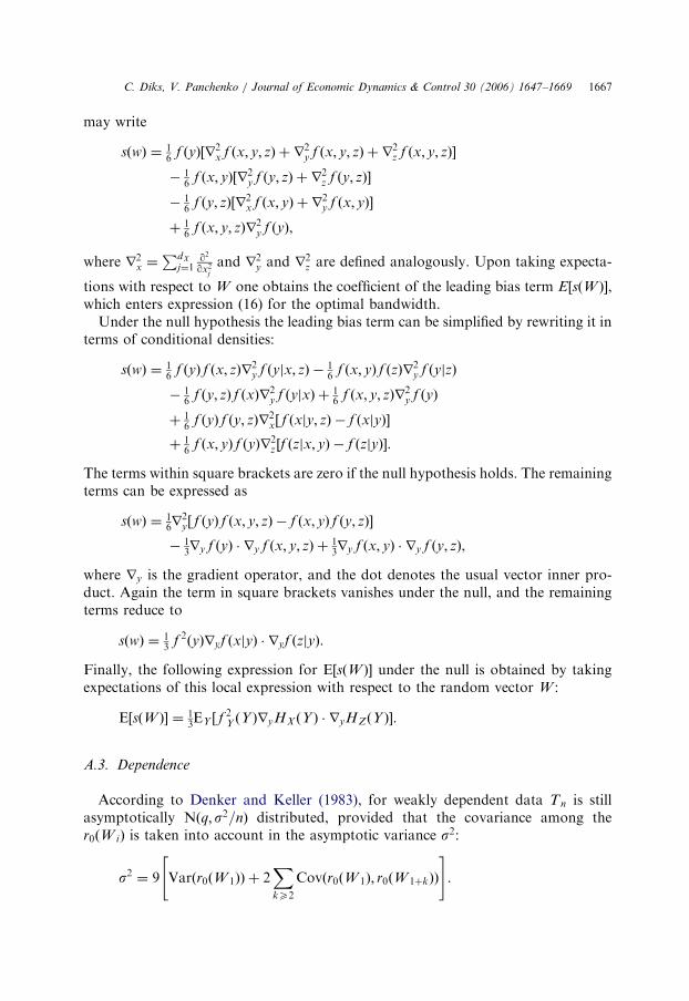
ARTICLE IN PRESS
C. Diks, V. Panchenko / Journal of Economic Dynamics & Control 30 (2006) 1647–1669 1667
may write
sðwÞ ¼ 16
f ðyÞ½r2x f ðx; y; zÞ þ r2
y f ðx; y; zÞ þ r2z f ðx; y; zÞ�
� 16
f ðx; yÞ½r2y f ðy; zÞ þ r2
z f ðy; zÞ�
� 16
f ðy; zÞ½r2x f ðx; yÞ þ r2
y f ðx; yÞ�
þ 16
f ðx; y; zÞr2y f ðyÞ,
where r2x ¼
PdX
j¼1q2
qx2j
and r2y and r2
z are defined analogously. Upon taking expecta-
tions with respect to W one obtains the coefficient of the leading bias term E½sðW Þ�,which enters expression (16) for the optimal bandwidth.
Under the null hypothesis the leading bias term can be simplified by rewriting it interms of conditional densities:
sðwÞ ¼ 16
f ðyÞ f ðx; zÞr2y f ðyjx; zÞ � 1
6f ðx; yÞ f ðzÞr2
y f ðyjzÞ
� 16
f ðy; zÞ f ðxÞr2y f ðyjxÞ þ 1
6f ðx; y; zÞr2
y f ðyÞ
þ 16
f ðyÞ f ðy; zÞr2x½ f ðxjy; zÞ � f ðxjyÞ�
þ 16
f ðx; yÞ f ðyÞr2z ½f ðzjx; yÞ � f ðzjyÞ�.
The terms within square brackets are zero if the null hypothesis holds. The remainingterms can be expressed as
sðwÞ ¼ 16r2
y½ f ðyÞ f ðx; y; zÞ � f ðx; yÞ f ðy; zÞ�
� 13ry f ðyÞ � ry f ðx; y; zÞ þ 1
3ry f ðx; yÞ � ry f ðy; zÞ,
where ry is the gradient operator, and the dot denotes the usual vector inner pro-duct. Again the term in square brackets vanishes under the null, and the remainingterms reduce to
sðwÞ ¼ 13
f 2ðyÞryf ðxjyÞ � ryf ðzjyÞ.
Finally, the following expression for E½sðW Þ� under the null is obtained by takingexpectations of this local expression with respect to the random vector W :
E½sðW Þ� ¼ 13EY ½ f
2Y ðY ÞryHX ðY Þ � ryHZðY Þ�.
A.3. Dependence
According to Denker and Keller (1983), for weakly dependent data Tn is stillasymptotically Nðq;s2=nÞ distributed, provided that the covariance among ther0ðW iÞ is taken into account in the asymptotic variance s2:
s2 ¼ 9 Varðr0ðW 1ÞÞ þ 2XkX2
Covðr0ðW 1Þ; r0ðW 1þkÞÞ
" #.
ARTICLE IN PRESS
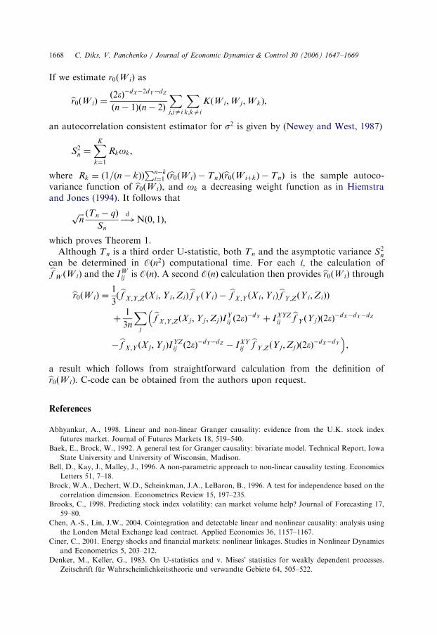
C. Diks, V. Panchenko / Journal of Economic Dynamics & Control 30 (2006) 1647–16691668
If we estimate r0ðW iÞ as
br0ðW iÞ ¼ð2eÞ�dX�2dY�dZ
ðn� 1Þðn� 2Þ
Xj;jai
Xk;kai
KðW i;W j ;W kÞ,
an autocorrelation consistent estimator for s2 is given by (Newey and West, 1987)
S2n ¼
XK
k¼1
Rkok,
where Rk ¼ ð1=ðn� kÞÞPn�k
i¼1 ðbr0ðW iÞ � TnÞðbr0ðW iþkÞ � TnÞ is the sample autoco-variance function of br0ðW iÞ, and ok a decreasing weight function as in Hiemstraand Jones (1994). It follows thatffiffiffi
np ðTn � qÞ
Sn
�!d
Nð0; 1Þ,
which proves Theorem 1.Although Tn is a third order U-statistic, both Tn and the asymptotic variance S2
n
can be determined in Oðn2Þ computational time. For each i, the calculation ofbf W ðW iÞ and the IWij is OðnÞ. A second OðnÞ calculation then provides br0ðW iÞ through
br0ðW iÞ ¼1
3ðbf X ;Y ;ZðX i;Y i;ZiÞ
bf Y ðY iÞ �bf X ;Y ðX i;Y iÞ
bf Y ;ZðY i;ZiÞÞ
þ1
3n
Xj
bf X ;Y ;ZðX j ;Y j ;ZjÞIYij ð2eÞ
�dY þ IXYZij
bf Y ðY jÞð2eÞ�dX�dY�dZ
��bf X ;Y ðX j ;Y jÞI
YZij ð2eÞ
�dY�dZ � IXYijbf Y ;ZðY j ;ZjÞð2eÞ
�dX�dY
,
a result which follows from straightforward calculation from the definition ofbr0ðW iÞ. C-code can be obtained from the authors upon request.
References
Abhyankar, A., 1998. Linear and non-linear Granger causality: evidence from the U.K. stock index
futures market. Journal of Futures Markets 18, 519–540.
Baek, E., Brock, W., 1992. A general test for Granger causality: bivariate model. Technical Report, Iowa
State University and University of Wisconsin, Madison.
Bell, D., Kay, J., Malley, J., 1996. A non-parametric approach to non-linear causality testing. Economics
Letters 51, 7–18.
Brock, W.A., Dechert, W.D., Scheinkman, J.A., LeBaron, B., 1996. A test for independence based on the
correlation dimension. Econometrics Review 15, 197–235.
Brooks, C., 1998. Predicting stock index volatility: can market volume help? Journal of Forecasting 17,
59–80.
Chen, A.-S., Lin, J.W., 2004. Cointegration and detectable linear and nonlinear causality: analysis using
the London Metal Exchange lead contract. Applied Economics 36, 1157–1167.
Ciner, C., 2001. Energy shocks and financial markets: nonlinear linkages. Studies in Nonlinear Dynamics
and Econometrics 5, 203–212.
Denker, M., Keller, G., 1983. On U-statistics and v. Mises’ statistics for weakly dependent processes.
Zeitschrift fur Wahrscheinlichkeitstheorie und verwandte Gebiete 64, 505–522.
ARTICLE IN PRESS
C. Diks, V. Panchenko / Journal of Economic Dynamics & Control 30 (2006) 1647–1669 1669
Diks, C., Panchenko, V., 2005. A note on the Hiemstra–Jones test for Granger non-causality. Studies in
Nonlinear Dynamics and Econometrics 9 (art. 4).
Engle, R., 1982. Autoregressive conditional heteroskedasticity with estimates of the variance of U.K.
inflation. Econometrica 50, 987–1008.
Granger, C.W.J., 1969. Investigating causal relations by econometric models and cross-spectral methods.
Econometrica 37, 424–438.
Hiemstra, C., Jones, J.D., 1994. Testing for linear and nonlinear Granger causality in the stock
price–volume relation. Journal of Finance 49, 1639–1664.
Ma, Y., Kanas, A., 2000. Testing for a nonlinear relationship among fundamentals and the exchange rates
in the ERM. Journal of International Money and Finance 19, 135–152.
Newey, W., West, K., 1987. A simple, positive semi-definite, heteroskedasticity and autocorrelation
consistent covariance matrix. Econometrica 55, 703–708.
Okunev, J., Wilson, P., Zurbruegg, R., 2000. The causal relationship between real estate and stock
markets. Journal of Real Estate Finance and Economics 21, 251–261.
Okunev, J., Wilson, P., Zurbruegg, R., 2002. Relationships between Australian real estate and stock
market prices – a case of market inefficiency. Journal of Forecasting 21, 181–192.
Politis, D.N., Romano, J.P., 1994. The stationary bootstrap. Journal of the American Statistical
Association 89, 1303–1313.
Pompe, B., 1993. Measuring statistical dependences in time series. Journal of Statistical Physics 73,
587–610.
Powell, J.L., Stoker, T.M., 1996. Optimal bandwidth choice for density-weighted averages. Journal of
Econometrics 75, 219–316.
Serfling, R.J., 1980. Approximation Theorems of Mathematical Statistics. Wiley, New York.
Silvapulla, P., Moosa, I.A., 1999. The relationship between spot and futures prices: evidence from the
crude oil market. Journal of Futures Markets 19, 157–193.
Skaug, H.J., Tjøstheim, D., 1993. Nonparametric tests of serial independence. In: Subba Rao, T. (Ed.),
Developments in Time Series Analysis. Chapman & Hall, London.
Su, L., White, H., 2003. A nonparametric Hellinger metric test for conditional independence. Technical
Report, Department of Economics, UCSD.


![William Lilly - Christian Astrology 1647 [Volume 1]](https://img.pdfslide.us/doc/110x75/547f132eb37959932b8b5793/william-lilly-christian-astrology-1647-volume-1.jpg)