Journal of Advances in Computer Engineering and Technology, 4(1) 2018

A New Optimized Hybrid Model Based on COCOMO to Increase the Accuracy of Software

Cost EstimationRamin Saljoughinejad1; Vahid Khatibi2

Received (2017-07-29)Accepted (2017-10-28)

Abstract — The literature review shows software development projects often neither meet time deadlines, nor run within the allocated budgets. One common reason can be the inaccurate cost estimation process, although several approaches have been proposed in this field. Recent research studies suggest that in order to increase the accuracy of this process, estimation models have to be revised. The Constructive Cost Model (COCOMO) has often been referred as an efficient model for software cost estimation. The popularity of COCOMO is due to its flexibility; it can be used in different environments and it covers a variety of factors. In this paper, we aim to improve the accuracy of cost estimation process by enhancing COCOMO model. To this end, we analyze the cost drivers using meta-heuristic algorithms. In this method, the improvement of COCOMO is distinctly done by effective selection of coefficients and reconstruction of COCOMO. Three meta-heuristic optimization algorithms are applied synthetically to enhance the process of COCOMO model. Eventually, results of the proposed method are compared to COCOMO itself and other existing models. This comparison explicitly reveals the superiority of the proposed method.

Index Terms — Accuracy, COCOMO 81, effort estimation, optimization, software project.

I. INTRODUCTION

With the evolution of computers, the role of software applications has increased. However, a study shows that 30% percent of projects were canceled, 84% were late or over budget (91% for larger companies), 52.7% cost an average of 189% over budget, the average system is delivered without 58% of the proposed functionalities, 81 billion dollars in 1995 was spent on cancelled projects, 51 billion dollars in 1995 was spent for over budget projects and only 16.2% of the software projects were completed on-time and on-budget [1].

An effective estimation gives a great deal of power to the project manager and helps to make better allocation decisions during the life cycle of the project. This includes telling other stakeholders of the software project how much effort is still needed to accomplish. With a faulty estimation, a software project leads to an inevitable defeat [1], [2].

Nowadays, there are many approaches to estimate software development effort, and it is up to the manager to choose one of the approaches depending on the type of the project. One of the most popular and known models is COCOMO. This model was introduced using constant parameters as well as applying statistical data regression analysis based on 63 various software projects. The Constructive Cost Model is an algorithmic software cost estimation model which is developed by Barry W. Boehm in 1981 and was first published in Boehm’s book “Software Engineering Economics” as a model for estimating cost, effort and schedule for software projects [3]. Although this model gives

1- Student of ACRCE Khozestan (ar.habibi69@gmail.com)2- Depatment of Computer, Central Tehran Branch, Islamic Azad University, Tehran, Iran.

28 Journal of Advances in Computer Engineering and Technology, 4(1) 2018

a good estimation, it is still away from the actual effort and cost [3]-[6]. The objective of this paper is to first review different types of COCOMO model and then to improve it. This paper is organized in 8 sections as follows: The literature review is presented in Section 2 and COCOMO is explained in Section 3. PSO, GA and IWO are elaborated in Section 4, 5 and 6, respectively. The proposed model is presented in Section 7 while the results are evaluated in Section 8. Finally, Conclusion and future work are explained in Section 9.

II. LITERATURE REVIEW

Estimating required resources for developing a software product plays a vital role in the management of software projects including resource allocation project programming and project auction. Various research studies highlight the importance of accurate estimation through introducing software cost estimation approaches. The following sub classes are categorized through a cognitive study which includes: COCOMO, lifelong, etc. [7].

F-COCOMO using fuzzy logic for software effort estimation is introduced by Fi & Liu [8]. The estimation capability is not yet spotted as no comparison has been made between fuzzy COCOMO and other effort estimation models. Rodger introduce a fuzzy COCOMO recognized as adaptive model of effort drivers, though its efficiency is not mentioned [8]. Audrey et al. define a fuzzy set for linguistic values of each effort driver by a trapezoidal membership function for fuzzy COCOMO. In the original model of COCOMO the fuzzy sets are the origin of obtained effort estimation coefficients. The fuzzy COCOMO is less sensitive toward software effort drivers relative to COCOMO81 [9]. A modeling approach of fuzzy linguistic effort estimation for confronting linguistic effort divers was presented by Zhu et al. which automatically generates fuzzy membership function through 81 COCOMO data set. The proposed fuzzy identifying model presents a more error free effort estimation compared to the 3 main models of COCOMO (basic, medium, accurate) [10]. Many models have received compliments for making relationship between size and effort in software cost estimation. Some of the applied methods in this regard include genetic algorithm

[11], fuzzy models [12], synthetic and dynamic models [13], neural networks [14], and basic regression [15]. Two common methods of cost estimation approaches include algorithm and non-algorithm approaches [16]. The algorithm method widely puts math skills in use from simple calculations or statistics to regression and differential equations [17]. On the other hand, non-algorithm approaches are analysis-based reasoning and learning, a study has recently been devoted to optimize the decision parameters in COCOMO through 81 NASA COCOMO data set [18]. Optimizing data set values, machine learning, analogy, data mining and neural networks were helped by different approaches [19]. In this regard, we have particle swarm optimization which is another approach used for optimizing [20], [21]. A multilayer neural network with 23nodes in hidden layer for effort estimation in software projects was presented by Da Silva D. Regression approach is also run in this approach for evaluating network and artificial data collection. The results were presented according to MMRE and PRED and compared with 2 COCOMO. As a result of the comparison shown, networks which were presented can create higher exact result [19], [22]. Soda et al. suggested two neurotic networks of RBF and GR for endeavor estimation of software project. 81 data collection of COCOMO is used in this project and the results of neural network are compared with the result that was obtained from COCOMO. The results show that both RBF and GR that are relative to COCOMO can display more exact results and RBF presented the best outcome [23]. Rady and Raju presented a feed forward neural network which consists of 22 neurons in the input layer, 2 hidden layers, and one node in the output layer. The basis of this architecture is on 17 COCOMO factor of effort and scale factor. COCOMO equation changed into linear equation, therefore, linear transfer function is chosen for the network. 81 COCOMO data collection was used for evaluating the performance of the network according to MMRE. 15 projects were randomly selected as the order set while others performed as test set. As shown by the obtained result compared with COCOMO results, the suggested network presented higher exact results [24]. Neural networks are widely used for estimating the objectives in different kinds of science. Moreover, it was used in software development effort estimation. Rao

Journal of Advances in Computer Engineering and Technology, 4(1) 2018 29

used functional link artificial neural networks for estimating efforts for software projects. Network architecture is considerably simple. In network architecture, we don’t have any hidden layers and learn how this type of neural works so quickly. According to COCOMO, this network cost 17 stimulations and 5 determined scale factors [25]. Reddy and Raju introduced feed forward neural network which consists of 22 neurons in the input layer, 2 hidden layer and one node in the output layer. This architecture is considered as (EMS15) according to COCOMO estimation and (5SFS) because of the scale factors. Therefore, COCOMO equation changed into linear equation and linear transfer function which were selected for network. According to MMRE, COCOMO 81 data collection was used to evaluate network performance. Totally, 50 projects act randomly as the trail set and the other projects act as the test set. Results of this test compared with COCOMO results show that estimating proposed network is more accurate [26]. Idri et al. look for an appropriate structure of radial basis function neural network and in particular the number of neurons in the hidden layer. This study focused on the level of accuracy in software projects under the influence of Gaussian function width [20]. One of the most popular methods to estimate software development effort is artificial neural networks and due to its popularity, several studies were carried out using neural networks in the past few years. Artificial neural network based models have shown that they can provide an appropriate estimation at the beginning of a project due to having access to the information from efforts of completed projects while model-based methods are not able to provide such an estimation due to limited project knowledge [27]. A new model based on using binary genetic algorithm was later introduced by Mirsa to estimate software effort for NASA supported projects. A modified version came out later considering the effect of methodology and using the COCOMO model to estimate effort which was able to provide appropriate estimation [28]. Particle swarm optimization is an algorithm developed to optimize a problem by trying to improve the candidate solution. The main advantage of this algorithm compared to many other global optimization algorithms such as Firefly and Genetic is its quick convergence. A later study by Sheta et al. used PSO to regulate COCOMO parameters by using soft calculation techniques in

order to estimate software effort better [19], [22]. A new model based on optimizing the COCOMO model by using TLBO algorithm introduced by S. K. Sehra, Y. S. Brar, N. Kaur, and G. Kaur. The results show this model’s superiority compared with four different models including SEL, Haltsead, Bailey-Basili and BCO [29].

1. COCOMO 81COCOMO 81 is a model that allows one to

estimate the effort, cost, and schedule when planning a new software development activity. It exists in three forms, each one offering greater detail and accuracy the further along one is in the project planning and design process. Listed by increasing fidelity, these forms are called Basic, Intermediate, and Detailed COCOMO [3]-[6].

1.1. Basic COCOMOBasic COCOMO estimates effort (and cost)

as a function of program size. Program size is expressed in terms of the number of the source lines of code divided by 1000 (SLOC, KLOC). Basic COCOMO applies to three kinds of software projects known as 1-Organic, which are “small” projects with “good” experience working with “less than rigid” requirements. 2-Semi-detached, “medium” teams with mixed experience working with a mix of rigid and less than rigid requirements. 3-Embedded, which are developed with a set of “tight” constraints. It is also a combination of organic and semi-detached projects. Basic COCOMO equations take the form:

Effort Applied (E) = ab(KLOC)bb [ person-months] Eq.1

Development Time (D) = cb(Effort Applied)db [months] Eq.2

People required (P) = Effort Applied / Development Time [count]

Eq.3

The coefficients ab, bb, cb and db are given in table 1.

30 Journal of Advances in Computer Engineering and Technology, 4(1) 2018

Table I: Basic model coefficients [3]Software project ab bb cb db

Organic 2.4 1.05 2.5 0.3 Semi-detached 3.0 1.12 2.5 0.35

Embedded 3.6 1.20 2.5 0.32

Basic COCOMO is good for an early effort and cost estimation but it does not account for the differences in some cases such as personnel quality, hardware constraints and experience, use of modern tools and techniques.

1.2. Intermediate COCOMOIntermediate COCOMO computes software

development effort as a function of program size and a set of “cost drivers” that include hardware, personnel, subjective assessment of the product and project attributes. This extension considers a set of four “cost drivers”, each with a number of subsidiary attributes which are 15 in total.

Each of the 15 attributes receives a rating on a six-point scale that ranges from “very low” to “extra high” (in importance or value). An effort multiplier from the table below applies to the rating. The product of all effort multipliers results in an effort adjustment factor (EAF). Typical values for EAF range from 0.9 to 1.4.

The Intermediate COCOMO formula now takes the form:

E=ai(KLoC)(bi)(EAF) Eq. 4

Where E is the effort applied in person-months, KLoC is the estimated number of thousands of delivered lines of code for the project, and EAF is the factor calculated above. The coefficient ai and the exponent bi are given in the following table.

Table 3: Intermediate model coefficients [3]Software project ai bi

Organic 3.2 1.05 Semi-detached 3.0 1.12

Embedded 2.8 1.20

1.3. Detailed COCOMODetailed COCOMO incorporates all

characteristics of the intermediate version with an assessment of the cost driver’s impact on each step (analysis, design, etc.) of the software engineering process.

The detailed model uses different effort

Table 2: Intermediate model cost drivers [3]Rating

Cost Drivers Extra High

Very High High Nominal Low Very

Low Product attributes

1.40 1.15 1 0.88 0.75 Required software reliability 1.60 1.08 1 0.94 Size of application database

1.65 1.30 1.15 1 0.85 0.70 Complexity of the product Hardware attributes

1.66 1.30 1.11 1 Run-time performance constraints 1.56 1.21 1.06 1 Memory constraints

1.30 1.15 1 0.87 Volatility of the virtual machine environment 1.15 1.07 1 0.87 Required turnabout time

Personnel attributes 0.71 0.86 1 1.19 1.46 Analyst capability 0.82 0.91 1 1.13 1.29 Applications experience 0.70 0.86 1 1.17 1.42 Software engineer capability 0.90 1 1.10 1.21 Virtual machine experience 0.95 1 1.07 1.14 Programming language experience

Project attributes 0.82 0.91 1 1.10 1.24 Application of software engineering methods 0.83 0.91 1 1.10 1.24 Use of software tools 1.10 1.04 1 1.08 1.23 Required development schedule

Journal of Advances in Computer Engineering and Technology, 4(1) 2018 31

multipliers for each cost driver attribute. These Phase Sensitive effort multipliers are each to determine the amount of effort required to complete each phase. In detailed COCOMO, the whole software is divided into different modules and then we apply COCOMO in different modules to estimate and then sum the effort.

In detailed COCOMO, the effort is calculated as a function of program size and a set of cost drivers given according to each phase of the software life cycle.

A Detailed project schedule is never static.

The five phases of detailed COCOMO are:• Plan and requirement• System design• Detailed design• Module code and test• Integration and test• Cost Constructive Model

III. PSO ALGORITHM

Particle swarm optimization (PSO) is a computational method that optimizes a problem by iteratively trying to improve a candidate solution with regard to a given measure of quality. PSO optimizes a problem by having a population of candidate solutions, here dubbed particles, and moving these particles around in the search-space according to simple mathematical formulae over the particle’s position and velocity. Each particle’s movement is influenced by its local best-known position but is also guided towards the best-known positions in the search-space, which are updated as better positions are found by other particles. This is expected to move the swarm towards the best solutions [4].

PSO is originally attributed to Kennedy, Eberhart and Shi and was first intended for simulating social behavior, as a stylized representation of the movement of organisms in a bird flock or fish school. The algorithm was simplified and it was observed to be performing optimization. The book by Kennedy and Eberhart describes many philosophical aspects of PSO and swarm intelligence [4], [30]. Table (4) shows the setting used for PSO algorithm in this paper.

Table 4: Setting for the PSO algorithm.Parameter Value

Npop 50 Itermax 500 Varmax 5 Varmin 0 Velmax (Varmax – Varmin) / 10 Velmin - Velmax

IV. GENETIC ALGORITHM

Genetic algorithm (GA) is a meta-heuristic algorithm inspired by the process of natural selection that belongs to the larger class of evolutionary algorithms (EA). Genetic algorithms are commonly used to generate high-quality solutions to optimization and search problems by relying on bio-inspired operators such as mutation, crossover and selection [31].

The evolution usually starts from a population of randomly generated individuals, and is an iterative process, with the population in each iteration called a generation. In each generation, the fitness of every individual in the population is evaluated; the fitness is usually the value of the objective function in the optimization problem being solved. The fitter individuals are stochastically selected from the current population, and each individual’s genome is modified (recombined and possibly randomly mutated) to form a new generation. The new generation of candidate solutions is then used in the next iteration of the algorithm. Commonly, the algorithm terminates when either a maximum number of generations has been produced or a satisfactory fitness level has been reached for the population [30], [31].

A typical genetic algorithm requires:1- a genetic representation of the solution

domain,2- a fitness function to evaluate the solution

domain.Once the genetic representation and the fitness

function are defined, a GA proceeds to initialize a population of solutions and then to improve it through repetitive application of the mutation, crossover, inversion and selection operators [31], [33]. The following table (table 5) shows the

Journal of Advances in Computer Engineering and Technology, 4(1) 2018 32

setting used for this algorithm in this paper.

Table 5: Setting for the genetic algorithm.Parameter Value

Ga_Pop_Size 50 Ga_Pop_evals 500

Ga_Elitism 1 Ga_Crossover_Rate 0.8 Ga_Mutation_Rate 0.02

V. INVASIVE WEED OPTIMIZATION ALGORITHM

Weeds are one of the most robust and troublous plants in agriculture. When you were young, you may have heard that ‘‘the weeds always win’’. This is due to the fact that the weeds have some strong properties, such as adaptation, robustness, vigorousness, and invasion. Based on those properties, a novel numerical stochastic optimization algorithm called invasive weed optimization (IWO) was proposed by Mehrabian and Lucas (2006) which is based on the natural selection (survival of the fittest) in the biological world [34].

To implement the IWO algorithm, there are many steps which are needed to be performed but the most important part of this algorithm is the “Spatial distribution” step. In this part, the generated seeds are being randomly distributed over the d-dimensional search space by normally distributed random numbers with a mean equal to zero; but varying variance parameters decreasing over the number of iteration. The reason for that is to guarantee that the produced seeds will be generated in a distant area but around the parent weed and decrease non-linearly, which results in grouping the fitter plants together and the inappropriate plants are eliminated over times.

Here, the standard deviation (s) of the random function is made to decrease over the iterations from a previously defined initial value (s initial), to a final value (s final), which is calculated in every time step via Equation (5).

𝜎𝜎���� � �������� � ����������������� �𝜎𝜎������� � �𝜎𝜎������ ��𝜎𝜎�����

Eq. 5

Where iter max is the maximum number of iterations, siter is the standard deviation at the present time step and n is the nonlinear modulation index usually set as 2.

Taking into account the key phases described above, the steps of implementing the IWO algorithm can be summarized as follows [34]:

• Step 1: Initialize randomly generated weeds in the entire search space.

• Step 2: Evaluate fitness of the whole population members.

• Step 3: Allow each population member to produce a number of seeds with better population members which in turn produce more seeds.

• Step 4: The generated seeds are distributed over the search space by normally distributed random numbers with a mean equal to zero but varying variance.

• Step 5: When the weed population exceeds the upper limit, perform competitive exclusion.

• Step 6: Check the termination criteria.

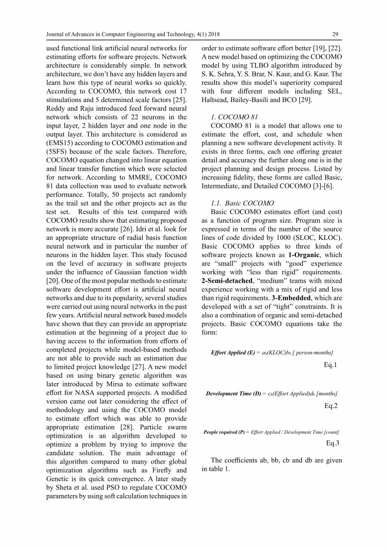
The following table (table 6) shows the setting used for this algorithm in this paper.

Table 6: Setting for the IWO algorithm.Parameter  Value

No 30 Itermax 500 Pmax 50 Smax 50 Smin 30 N 3

Ϭinitial 5 ϬFinal 0.5

VI. THE PURPOSED METHOD

The information related to the proposed method is presented in this section. The present synthetic approach tries to obtain the best estimation as much as possible through improving the attributes and COCOMO coefficient optimization. The procedure of synthesizing different sections of the proposed model is carried out in a way that the estimation error decreases. The proposed method consists of three main sections each of which includes a model training section and a

Journal of Advances in Computer Engineering and Technology, 4(1) 2018 33

model testing section elaborated in the following sections:

1. Section1: An effective selection of coefficients using meta-heuristic algorithms

1.1. Section 1 Model trainingA part of the proposed method is generated

and configured in this section. The parameters of the proposed method, a and b parameters in COCOMO are indeed set in this section and the goal is to produce optimized coefficients. In the beginning, all the projects are randomly divided into two groups of training and testing. And then, each of these groups are divided into three other groups which are Organized, Semi-detached and Embedded according to COCOMO formula, this dividing is due to the heterogeneity of COCOMO projects. After dividing the training data into three groups, meta-heuristic algorithms are used to optimize the coefficients to minimize the estimation effort of each project. Through optimization of coefficients (6) formula is used as the fitness function for all the meta-heuristic algorithms.

Effort = | Real Cost – Estimation Cost | Eq. 6

In this formula, it has been tried to minimize the estimated effort to increase the accuracy of the COCOMO. The reason for using the same fitness function for all meta-heuristic algorithms is to test them all under equal conditions.

It also needs to be mentioned that apart from using these algorithms separately, the two IWO and PSO algorithms are also used in combination. It means that the result of PSO algorithm has been used as a part of the IWO population. The reason for this is to increase the accuracy of IWO algorithm and test these two algorithms together.

Performance parameters in all the sections are MMRE and PRED. For estimating MMRE and PRED, first MRE should be estimated through the following formula.

��� � � ��𝐴𝐴��𝐴𝐴𝐴𝐴�� � 𝐴𝐴𝐴𝐴𝐴𝐴𝐴𝐴𝐴𝐴𝐴𝐴 �𝐴𝐴𝐴𝐴𝐴𝐴𝐴𝐴𝐴𝐴𝐴𝐴 Eq. 7

After MRE’s estimation for all projects, MMRE and PRED values are estimated through (8) and (9) formula.

𝑀𝑀𝑀𝑀𝑀𝑀𝑀𝑀 � ∑ 𝑀𝑀𝑀𝑀𝑀𝑀����N Eq. 8

𝑃𝑃𝑃𝑃𝑃𝑃𝑃𝑃�𝑥𝑥� � 𝐴𝐴𝑁𝑁 Eq. 9

The value of MMRE equals to the average of MREs in a single group (organic, semi-detached or embedded). The value of PRED equals to the percentage of the projects the MRE value of which is less than or equal to X, and N is the number of estimated projects. The acceptable value of X is 0.25 according to which the proposed methods are compared. MMRE as the total value of error in projects should be minimized whereas PRED (0.25) should be maximized.

Fig.1. Training stage in proposed model (Section 1)

1.2. Section 1 Model TestingIn this section, the results of training section (a,

b coefficients) are used to evaluate the proposed method. Data used in this section are the testing

Journal of Advances in Computer Engineering and Technology, 4(1) 2018 34

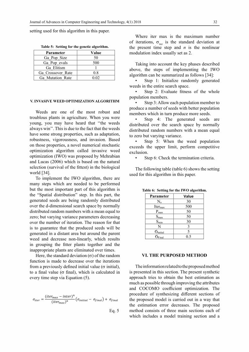
data. First, all the testing projects are divided into three classes of Organic, semi-detached and embedded according to the COCOMO project types. After class identification of the projects, the related coefficients of the project are extracted and then used to estimate the effort of each project. After the calculation of the effort for all the testing projects, The MRE related to testing projects is estimated and then in evaluation part MMRE and PRED are estimated. All These processes are shown in Fig (2).

Fig. 2. Testing stage in proposed model (Section 1)

2. Section 2: Cost Drivers Optimization using meta-heuristic algorithms

2.1. Section 2 Model TrainingAt this step, we try to optimize cost drivers

using meta-heuristic algorithms in order to reach better factors for optimizing the answer of suggested model by reapplying the first step on these drivers. As the number of drivers is 15 and each is different, first project categories are

formed at this phase. The projects have the same amount in one feature are categorized in one group. For example, all the projects that have “very little” amount in reliability feature needed for the software in one category. The projects that have little amount in another, and the projects that have average amount are categorized in another groups. The categorization is done for all features and amounts. Then according to the result of the previous step using the IWO, PSO algorithms, we optimize the drivers at the category. As it is always tried to reduce the amount of MMRE and increase the PRED in each category. Through optimization of cost drivers (6) formula is used as the fitness function for our two meta-heuristic algorithms. And all these processes are shown in Fig (3).

Fitness = | MMRE – PRED | Eq. 10

Fig.3. Training stage in proposed model (Section 2)

Journal of Advances in Computer Engineering and Technology, 4(1) 2018 35

2.2. Section 2 Model TestingIn this section, the result of training section

which is a table of new Cost Drivers is used to evaluate the proposed method. Data used in this section are the testing data. After dividing all the projects into the three groups of Organic, Semi-detached and Embedded the cost drivers of each project are replaced with their corresponding cost drive from the results of training section to estimate the effort of each project. After the calculation of the effort for all the testing projects, The MRE related to testing projects is estimated and then in evaluation part MMRE and PRED are estimated. All These processes are shown in Fig (4).

Fig.4. Testing stage in proposed model (Section 2)

3. Section3: An effective selection of coefficients using the new cost drivers from section 2, and meta-heuristic algorithms

3.1. Section 3 Model TrainingAll the steps in this section are the same as

those which are in section 1 and the goal again

is to produce optimized coefficients; the only difference in this section is that the cost drivers which are used here are the results of section 2. First, all the projects are divided into three groups of Organic, Semi-detached, Embedded, then the cost drivers of each project are replaced with their corresponding cost drive from the results of section 2. After replacing the cost drivers the three meta-heuristic algorithms are used to optimize the coefficients to minimize the estimation effort of each project. All These processes are shown in Fig (5).

Fig.5. Training stage in proposed model (Section 3)

3.2. Model TestingThis part is exactly the same as the model

testing part in section 1. All These processes are shown in Fig (6).

Journal of Advances in Computer Engineering and Technology, 4(1) 2018 36

Fig. 6. Testing stage in proposed model (Section 3)

VII. RESULTS EVALUATION

In this section, the performance of the proposed method is evaluated applying the data related to the real projects. The evaluation stage consists of three main sections each of which includes 3 different parts as the COCOMO method has 3 different types for projects. The results of all these three sections are shown and then compared to the COCOMO results themselves.

1. Section 1 Evaluation

Table7: Obtained results from organic projects (Section1) A B MMRE PRED MMRE-

PRED PSO 1.834 1.472 1.408 0.125 1.283

GENETIC 1.966 1.452 1.417 0 1.417 IWO 2.018 1.353 0.868 0.25 0.618

PSO + IWO 2.743 1.002 0.209 0.75 -0.541 COCOMO 3.2 1.05 0.299 0.625 -0.326

Table (7) shows the results related to organic projects. In this table, a and b coefficients, MMRE and PRED performance criteria, and the subtraction of MMRE and PRED performance criteria for all algorithms are presented. As indicated by the results, a’s coefficients range is from 1.834 to 3.2 and b’s coefficients range is from 1.002 to 1.472.

The MMRE range for these projects is from 0.209 to 1.417. The best MMRE for these projects is 0.209, which is the result of the combination of two IWO and PSO algorithms. The PRED range for these projects is from 0 to 0.75, and again the best PRED is the result of combining the two IWO and PSO algorithms which is 0.75.

Table 8: Obtained results from semi-detached projects (Section1)

A B MMRE PRED MMRE-PRED

PSO 1.732 1.215 0.395 0.571 -0.176 GENETIC 2.471 1.352 2.270 0 2.270

IWO 2.020 1.337 1.467 0.286 1.181 PSO + IWO 2.412 1.121 0.26 0.286 -0.025 COCOMO 3.0 1.12 0.326 0.571 -0.245

Table (8) shows the results related to semi-detached projects. As indicated by the results, a’s coefficients range is from 1.732 to 3.0 and b’s coefficients range is from 1.12 to 1.352.

The MMRE range for these projects is from 0.26 to 2.27. The best MMRE for these projects is 0.26, which is the result of the combination of two IWO and PSO algorithms. The PRED range for these projects is from 0 to 0.571. The best PRED is the result of PSO algorithms, which is 0.571.

Table 9: Obtained results from embedded projects

(Section 1) A B MMRE PRED MMRE

-PRED PSO 1.142 1.531 0.295 0.4 -0.105

GENETIC 1. 102 1.52 0.550 0.2 0.350 IWO 1.971 1.372 0.327 0.3 0.026

PSO + IWO 2.873 1.181 0.266 0.5 -0.234 COCOMO 2.8 1.20 0.258 0.6 -0.341

Table (9) shows the results related to embedded projects. As indicated by the results, a’s coefficients range is from 1.102 to 2.873 and b’s coefficients range is from 1.181 to 1.531. The MMRE range for these projects is from 0.258 to 0.550. The best MMRE for these projects

Journal of Advances in Computer Engineering and Technology, 4(1) 2018 37

is 0.258, which is the result of the COCOMO model. The PRED range for these projects is from 0 to 0.6, and again the best PRED is the result of COCOMO model which is 0.6.

Results related to the proposed method (Section 1) are presented in tables 4, 5, and 6. The best PRED value has obtained for organic projects indicating the influence of coefficients optimization on increasing the percentage of estimation in these projects. The best value of MMRE has obtained again for organic projects and it is probably because of the large number of these projects. The important point is the notable difference of the proposed coefficients for all three kinds of projects caused by projects variation.

2. Section 2 Evaluation

Table10: Obtained results from all groups of projects (Section 2)

Organic MMRE PRED MMRE-PRED

New Model 0.274 0.5 -0.225

COCOMO 0.342 0.541 -0.199

Semi-detached MMRE PRED MMRE-PRED

New Model 0.242 0.428 -0.186

COCOMO 0.295 0.636 -0.341

Embedded MMRE PRED MMRE-PRED

New Model 0.267 0.6 -0.332

COCOMO 0.316 0.535 -0.218-

Table (10) shows the result related to all the three project types. As indicated by the results, the proposed method has achieved a better estimation both in organic and embedded projects than COCOMO model itself, this represents better cost drivers in the proposed method compared to the COCOMO model. All these new cost drivers are presented in table (11).

3. Section 3 Evaluation

Table12: Obtained results from organic projects (Section3)

A B MMRE PRED MMRE-PRED

PSO 4.99 0.88 0.29 0.5 -0.21 IWO 4.27 0.93 0.30 0.549 -0.24

PSO + IWO 4.99 0.88 0.29 0.5 -0.21 COCOMO 3.2 1.05 0.34 0.54 -0.19

Table (12) shows the results related to organic projects. As indicated by the results, a’s coefficients range is from 3.2 to 4.99 and b’s coefficients range is from 0.88 to 1.05.

The MMRE range for these projects is from 0.29 to 0.34. The best MMRE for these projects is 0.29, which is the result of the combination of two IWO and PSO algorithms. The PRED range for these projects is from 0.5 to 0.549 and it is the result of IWO algorithm, which is 0.549.

Table11: New cost drivers table for Intermediate projects in proposed modelRating

Cost Drivers Extra High

Very High High Nominal Low Very

Low Product attributes

1.43 1.12 0.98 0.90 0.73 Required software reliability 1.15 1.09 0.96 0.94 Size of application database

1.67 1.28 1.13 1.01 0.82 0.68 Complexity of the product Hardware attributes

1.65 1.28 1.09 1.02 Run-time performance constraints 1.55 1.22 1.03 0.98 Memory constraints

1.31 1.316 0.99 0.89 Volatility of the virtual machine environment 1.17 1.05 0.98 0.87 Required turnabout time

Personnel attributes 0.73 0.84 1 1.21 1.47 Analyst capability 0.83 0.90 0.99 1.11 1.25 Applications experience 0.68 0.87 0.97 1.15 1.39 Software engineer capability 0.87 0.97 0.99 1.19 Virtual machine experience 0.97 0.98 1.05 1.16 Programming language experience

Project attributes 0.80 0.89 0.99 0.98 1.25 Application of software engineering methods 0.81 0.88 1 0.98 1.25 Use of software tools 1.12 0.99 0.98 1.03 1.25 Required development schedule

Journal of Advances in Computer Engineering and Technology, 4(1) 2018 38

Table 13: Obtained results from semi-detached projects (Section 3)

A B MMRE PRED MMRE-PRED

PSO 4.83 1 0.19 0.73 -0.53 IWO 3.46 1.12 0.27 0.73 -0.46

PSO + IWO 4.83 1 0.19 0.73 -0.53 COCOMO 3.0 1.12 0.29 0.64 -0.34

Table (13) shows the results related to semi-detached projects. As indicated by the results, a’s coefficients range is from 3.0 to 4.83 and b’s coefficients range is from 1.00 to 1.12.

The MMRE range for these projects is from 0.19 to 0.29 and the best MMRE for these projects is 0.19, which is achieved by both PSO algorithm and the combination of two IWO and PSO algorithms. The PRED range for these projects is from 0.64 to 0.73 and as the table shows all the meta-heuristic algorithm achieved the same result.

Table14: Obtained results from embedded projects (Section 3)

A B MMRE PRED MMRE-PRED

PSO 1.56 1.31 0.41 0.32 0.09 IWO 1.24 1.45 0.49 0.46 0.03

PSO + IWO 1.56 1.31 0.41 0.32 0.09 COCOMO 2.8 1.20 0.32 0.53 -0.22

Table (14) shows the results related to embedded projects. As indicated by the results, a’s coefficients range is from 1.24 to 2.8 and b’s coefficients range is from 1.20 to 1.45.

The MMRE range for these projects is from 0.32 to 0.49. The best MMRE for these projects is 0.32, which is the result of the COCOMO model. The PRED range for these projects is from 0.32 to 0.53 and again the best result is achieved by COCOMO model itself.

4. Final proposed methodBy comparing the results of all three sections it

can be concluded that the best results for organic projects are those made in the first section. In other words we can achieve a better estimation for organic projects just by using the coefficients made in section one.

From the results of section three and

comparing them with the other two sections it can be concluded that the best results for semi-detached projects are those made in the third section. It means that by using the new cost drivers from section 2 and coefficients from section 3 we can achieve a better estimation for this type of projects.

By comparing the results of section three with the other two sections it can be concluded that the best results for embedded projects are those made in the second section, and we can achieve a better estimation just by using the new cost drivers from section two and COCOMO coefficients themselves.

We can generally deduce that the proposed model which is a combination of obtained results from all the three sections has the best cost estimation among all categories. It is, therefore, better to estimate the project utilizing following offered methods after the specification of the project type.

Proposed Method for Organic Projects• Using the new coefficients from section 1

(table 7)• Using the COCOMO’s model cost drivers

(table 2)

Proposed Method for Semi-detached Projects

• Using the new cost drivers from section 2 (table 11)

• Using the new coefficients from section 3 (table 13)

Proposed Method for Embedded Projects• Using the new cost drivers from section 2

(table 11)• Using the COCOMO’s model coefficients

(table 3)

5. Model EvaluationThe results of a valid article published in

2016 have been applied in order to evaluate the proposed method. At this stage, the performance measures (MMRE and PRED) have been used as well to make this evaluation [19].

Journal of Advances in Computer Engineering and Technology, 4(1) 2018 39

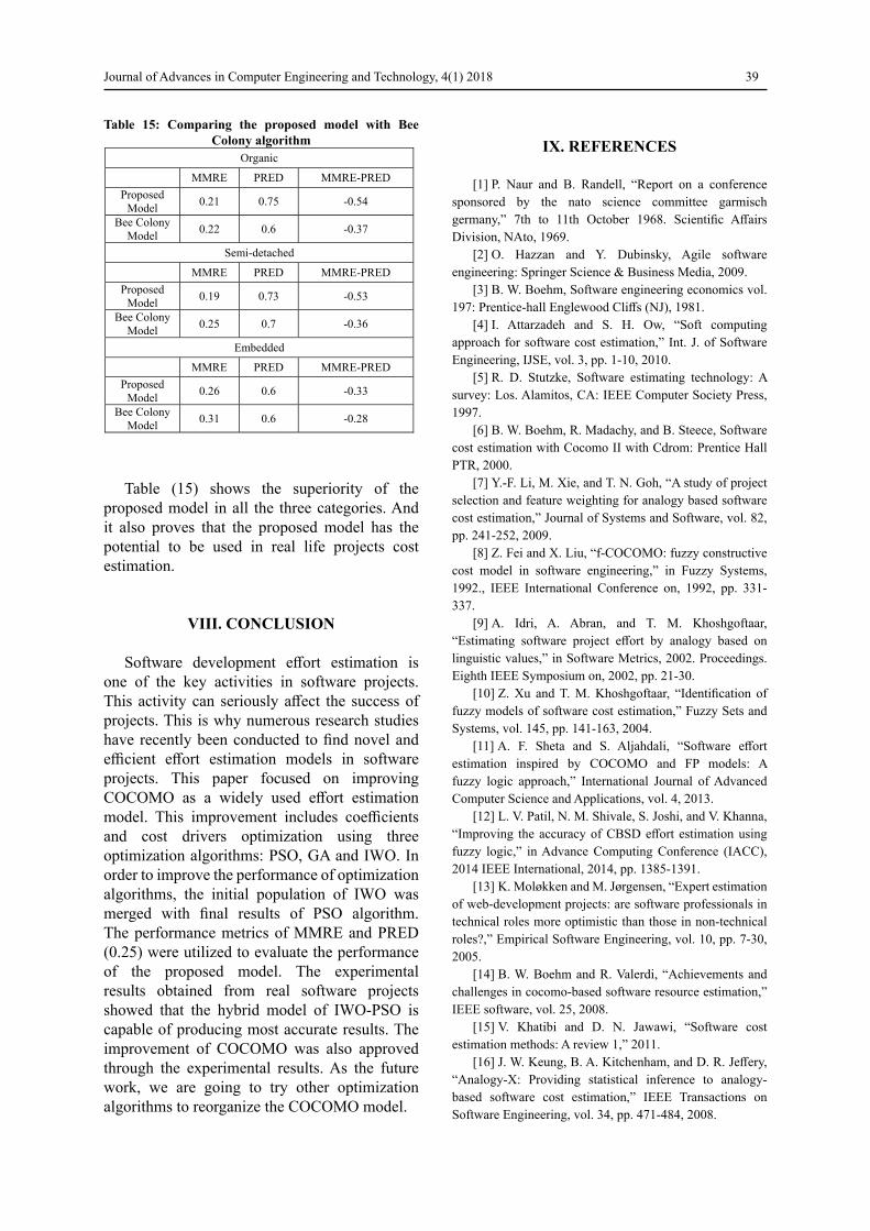
Table 15: Comparing the proposed model with Bee Colony algorithm

Organic MMRE PRED MMRE-PRED

Proposed Model 0.21 0.75 -0.54

Bee Colony Model 0.22 0.6 -0.37

Semi-detached MMRE PRED MMRE-PRED

Proposed Model 0.19 0.73 -0.53

Bee Colony Model 0.25 0.7 -0.36

Embedded MMRE PRED MMRE-PRED

Proposed Model 0.26 0.6 -0.33

Bee Colony Model 0.31 0.6 -0.28

Table (15) shows the superiority of the proposed model in all the three categories. And it also proves that the proposed model has the potential to be used in real life projects cost estimation.

VIII. CONCLUSION

Software development effort estimation is one of the key activities in software projects. This activity can seriously affect the success of projects. This is why numerous research studies have recently been conducted to find novel and efficient effort estimation models in software projects. This paper focused on improving COCOMO as a widely used effort estimation model. This improvement includes coefficients and cost drivers optimization using three optimization algorithms: PSO, GA and IWO. In order to improve the performance of optimization algorithms, the initial population of IWO was merged with final results of PSO algorithm. The performance metrics of MMRE and PRED (0.25) were utilized to evaluate the performance of the proposed model. The experimental results obtained from real software projects showed that the hybrid model of IWO-PSO is capable of producing most accurate results. The improvement of COCOMO was also approved through the experimental results. As the future work, we are going to try other optimization algorithms to reorganize the COCOMO model.

IX. REFERENCES

[1] P. Naur and B. Randell, “Report on a conference sponsored by the nato science committee garmisch germany,” 7th to 11th October 1968. Scientific Affairs Division, NAto, 1969.

[2] O. Hazzan and Y. Dubinsky, Agile software engineering: Springer Science & Business Media, 2009.

[3] B. W. Boehm, Software engineering economics vol. 197: Prentice-hall Englewood Cliffs (NJ), 1981.

[4] I. Attarzadeh and S. H. Ow, “Soft computing approach for software cost estimation,” Int. J. of Software Engineering, IJSE, vol. 3, pp. 1-10, 2010.

[5] R. D. Stutzke, Software estimating technology: A survey: Los. Alamitos, CA: IEEE Computer Society Press, 1997.

[6] B. W. Boehm, R. Madachy, and B. Steece, Software cost estimation with Cocomo II with Cdrom: Prentice Hall PTR, 2000.

[7] Y.-F. Li, M. Xie, and T. N. Goh, “A study of project selection and feature weighting for analogy based software cost estimation,” Journal of Systems and Software, vol. 82, pp. 241-252, 2009.

[8] Z. Fei and X. Liu, “f-COCOMO: fuzzy constructive cost model in software engineering,” in Fuzzy Systems, 1992., IEEE International Conference on, 1992, pp. 331-337.

[9] A. Idri, A. Abran, and T. M. Khoshgoftaar, “Estimating software project effort by analogy based on linguistic values,” in Software Metrics, 2002. Proceedings. Eighth IEEE Symposium on, 2002, pp. 21-30.

[10] Z. Xu and T. M. Khoshgoftaar, “Identification of fuzzy models of software cost estimation,” Fuzzy Sets and Systems, vol. 145, pp. 141-163, 2004.

[11] A. F. Sheta and S. Aljahdali, “Software effort estimation inspired by COCOMO and FP models: A fuzzy logic approach,” International Journal of Advanced Computer Science and Applications, vol. 4, 2013.

[12] L. V. Patil, N. M. Shivale, S. Joshi, and V. Khanna, “Improving the accuracy of CBSD effort estimation using fuzzy logic,” in Advance Computing Conference (IACC), 2014 IEEE International, 2014, pp. 1385-1391.

[13] K. Moløkken and M. Jørgensen, “Expert estimation of web-development projects: are software professionals in technical roles more optimistic than those in non-technical roles?,” Empirical Software Engineering, vol. 10, pp. 7-30, 2005.

[14] B. W. Boehm and R. Valerdi, “Achievements and challenges in cocomo-based software resource estimation,” IEEE software, vol. 25, 2008.

[15] V. Khatibi and D. N. Jawawi, “Software cost estimation methods: A review 1,” 2011.

[16] J. W. Keung, B. A. Kitchenham, and D. R. Jeffery, “Analogy-X: Providing statistical inference to analogy-based software cost estimation,” IEEE Transactions on Software Engineering, vol. 34, pp. 471-484, 2008.

Journal of Advances in Computer Engineering and Technology, 4(1) 2018 40

[17] C.-c. Lai and W.-l. Lee, “A WICE approach to real-time construction cost estimation,” Automation in Construction, vol. 15, pp. 12-19, 2006.

[18] G.-H. Kim, S.-H. An, and K.-I. Kang, “Comparison of construction cost estimating models based on regression analysis, neural networks, and case-based reasoning,” Building and environment, vol. 39, pp. 1235-1242, 2004.

[19] V. Khatibi Bardsiri and M. Dorosti, “An Improved COCOMO based Model to Estimate the Effort of Software Projects,” Journal of Advances in Computer Engineering and Technology, vol. 2, pp. 11-22, 2016.

[20] E. Khatibi, “Investigating the effect of software project type on accuracy of software development effort estimation in COCOMO model,” in Fourth International Conference on Machine Vision (ICMV 11), 2011, pp. 83500G-83500G-7.

[21] A. Idri, A. Zakrani, and A. Zahi, “Design of radial basis function neural networks for software effort estimation,” IJCSI International Journal of Computer Science Issues, vol. 7, 2010.

[22] G. S. Sandhu and D. S. Salaria, “A Bayesian Network Model of the Particle Swarm Optimization for Software Effort Estimation,” International Journal of Computer Applications, vol. 96, 2014.

[23] A. Dhiman and C. Diwaker, “Optimization of COCOMO II effort estimation using genetic algorithm,” American International Journal of Research in Science, Technology, Engineering & Mathematics, vol. 3, 2013.

[24] D. Karaboga, “An idea based on honey bee swarm for numerical optimization,” Technical report-tr06, Erciyes university, engineering faculty, computer engineering department2005.

[25] B. T. Rao, B. Sameet, G. K. Swathi, K. V. Gupta, C. RaviTeja, and S. Sumana, “A novel neural network approach for software cost estimation using Functional Link Artificial Neural Network (FLANN),” International Journal of Computer Science and Network Security, vol. 9, pp. 126-131, 2009.

[26] C. S. Reddy and K. Raju, “A concise neural network model for estimating software effort,” International Journal of Recent Trends in Engineering, vol. 1, pp. 188-193, 2009.

[27] B. K. Singh and A. Misra, “Software effort estimation by genetic algorithm tuned parameters of modified constructive cost model for nasa software projects,” International Journal of Computer Applications, vol. 59, 2012.

[28] V. K. Bardsiri, D. N. A. Jawawi, S. Z. M. Hashim, and E. Khatibi, “A PSO-based model to increase the accuracy of software development effort estimation,” Software Quality Journal, vol. 21, pp. 501-526, 2013.

[29] S. K. Sehra, Y. S. Brar, N. Kaur, and G. Kaur, “Optimization of COCOMO Parameters using TLBO Algorithm,” International Journal of Computational Intelligence Research, vol. 13, pp. 525-535, 2017.

[30] R. Eberhart and J. Kennedy, “A new optimizer using particle swarm theory,” in Micro Machine and Human Science, 1995. MHS’95., Proceedings of the Sixth International Symposium on, 1995, pp. 39-43.

[31] Y. Shi and R. Eberhart, “A modified particle swarm optimizer,” in Evolutionary Computation Proceedings, 1998. IEEE World Congress on Computational Intelligence., The 1998 IEEE International Conference on, 1998, pp. 69-73.

[32] J. Kennedy, “The particle swarm: social adaptation of knowledge,” in Evolutionary Computation, 1997., IEEE International Conference on, 1997, pp. 303-308.

[33] D. Goldberg, “Genetic algorithms in optimization, search and machine learning,” Reading: Addison-Wesley, 1989.

[34] L. M. Schmitt, “Theory of genetic algorithms,” Theoretical Computer Science, vol. 259, pp. 1-61, 2001.