A new model reference control architecture: stability ...lacis.eng.usf.edu/resources/RNC3416.pdf · DOI: 10.1002/rnc.3416 A new model reference control architecture: Stability, performance,

INTERNATIONAL JOURNAL OF ROBUST AND NONLINEAR CONTROLInt. J. Robust Nonlinear Control (2015)Published online in Wiley Online Library (wileyonlinelibrary.com). DOI: 10.1002/rnc.3416

A new model reference control architecture: Stability,performance, and robustness

Gerardo De La Torre1, Tansel Yucelen2,*,† and Eric N. Johnson1

1School of Aerospace Engineering, Georgia Institute of Technology, Atlanta, GA 30332, USA2Department of Mechanical and Aerospace Engineering, Missouri University of Science and Technology, Rolla,

MO 65409, USA

SUMMARY

In this paper, we develop a new model reference control architecture to effectively suppress system uncer-tainties and achieve a guaranteed transient and steady-state system performance. Unlike traditional robustcontrol frameworks, only a parameterization of the system uncertainty given by unknown weights withknown conservative bounds is needed to stabilize uncertain dynamical systems with predictable system per-formance. In addition, the proposed architecture’s performance is not dependent on the level of conservatismof the bounds of system uncertainty. Following the same train of thought as adaptive controllers that mod-ify a given reference system to improve system performance, the proposed method is inspired by a recentlydeveloped command governor theory that minimizes the effect of system uncertainty by augmenting theinput signal of the uncertain dynamical and reference systems. Specifically, a dynamical system, calleda command governor, is designed such that its output is used to modify the input of both the controlleduncertain dynamical and reference systems. It is theoretically shown that if the command governor designparameter is judiciously selected, then the controlled system approximates the given original, unmodifiedreference system. The proposed approach is advantageous over model reference adaptive control approachesbecause linearity of the uncertain dynamical system is preserved through linear control laws, and hence, theclosed-loop performance is predictable for different command spectrums. Additionally, it is shown that thearchitecture can be modified for robustness improvements with respect to high frequency content due to, forexample, measurement noise. Modifications can also be made in order to accommodate actuator dynamicsand retain closed-loop stability and predictable performance. The main contribution of this paper is the rig-orous analysis of the stability and performance of a system utilizing the command governor framework. Anumerical example is provided to illustrate the effectiveness of the proposed architecture. Copyright © 2015John Wiley & Sons, Ltd.

Received 1 June 2015; Accepted 3 August 2015

KEY WORDS: model reference control; command governor; uncertain dynamical systems; transient andsteady-state system performance; robustness

1. INTRODUCTION

There have been many control architectures formulated in order to address the important issue ofsystem uncertainty. These control architectures attempt to suppress the effect of system uncertaintyin order to achieve closed-loop stability and, in some cases, guaranteed system performance. Themajority of these controllers can be placed into two distinct categories, namely, robust and adap-tive control architectures. Robust controllers rely on mathematical models that precisely captureuncertain parameter variations in terms of lower and upper bounds. Once a set of all possible uncer-tainties are established, a control law is created in order to maintain closed-loop stability over the

*Correspondence to: Tansel Yucelen, Department of Mechanical and Aerospace Engineering, Missouri University ofScience and Technology, Rolla, MO 65409, USA.

†E-mail: [email protected]

Copyright © 2015 John Wiley & Sons, Ltd.

G. DE LA TORRE, T. YUCELEN AND E. N. JOHNSON

entire set [1]. Characterization of the set of all possible uncertainty, like the original problem of sys-tem identification, can be difficult and costly (e.g., aerospace applications [2, 3]). Therefore, overlyconservative sets are often used in order to guarantee closed-loop system stability. It has been estab-lished that the performance of a system controlled with a robust framework is directly affected bythe conservatism of the set of all possible uncertainties [4]. As a result, robust controllers tend to becautious and have relatively poor performance in the presence of high uncertainty.

On the other hand, adaptive controllers do not require complete knowledge of all possible uncer-tainties. Only knowledge of a parameterization of the system uncertainty given by an unknown idealweight matrix and a known basis function is required to suppress the effects of system uncertaintiesand failures [5–11]. The adaptive control framework either attempts, through feedback, to identifythe system uncertainty or dynamically changes its control law in order to suppress system uncer-tainty. This framework has been shown to be effective for tracking the states (or the outputs) of agiven ideal reference system capturing a desired closed-loop system behavior. Inherently, the adap-tive control law makes the overall closed-loop system nonlinear. Therefore, computing relative gainand time-delay margins for verification and validation purposes using linear system techniques isnot an easy task, and predicting transient and steady-state performance is challenging [12, 13].

The contribution of this paper is to present a new model reference control architecture that hasthe capability to effectively suppress system uncertainties and simultaneously achieve a guaranteedtransient and steady-state system performance. In particular, unlike traditional robust control frame-works, only a parameterization of the system uncertainty given by unknown weights with knownconservative bounds is needed to stabilize uncertain dynamical systems with predictable systemperformance. In addition, the proposed architecture’s performance is not dependent on the level ofconservatism of the bounds of system uncertainty. Following the same train of thought as adap-tive controllers that modify a given reference system to improve system performance, the proposedmethod is inspired by a recently developed command governor theory that minimizes the effect ofsystem uncertainty by augmenting the input signal of the uncertain dynamical system and a refer-ence system [2, 14–18]. Specifically, a dynamical system, called a command governor, is designedsuch that its output is used to modify the input of both the controlled uncertain dynamical andreference systems.

For the proposed model reference control architecture, it is theoretically shown that if the designparameter of the employed command governor is judiciously selected, then the controlled sys-tem approximates the given unmodified reference system. This implies that the tracking error withrespect to the original, unmodified reference system can be made arbitrarily small in the presenceof system uncertainties by altering the inputs of the controlled and reference systems. The proposedapproach is advantageous over model reference adaptive control approaches because linearity ofthe uncertain dynamical system is preserved through linear control laws, and hence, the closed-loop performance is predictable for different command spectrums. Additionally, it is shown that thearchitecture can be modified for robustness improvements with respect to high frequency contentdue to, for example, measurement noise. Modifications can also be made in order to accommodateactuator dynamics and retain closed-loop stability and predictable performance. The main contribu-tion of this paper is the rigorous analysis of the stability and performance of a system utilizing thecommand governor framework.

The paper is organized as follows. Section 2 outlines the notation and mathematical preliminar-ies used throughout the paper, and Section 3 presents the problem formulation and introduces theproposed model reference controller architecture based on the aforementioned command governor.In Section 4, the problem is placed into a robust control framework, and conditions for closed-loopstability are derived. Section 5 shows that the proposed architecture shapes the transient systemresponse of the controlled uncertain dynamical system such that it approximates the given idealreference system. Framework modifications in order to improve robustness with respect to high fre-quency system content and address the issue of actuator dynamics are presented in Sections 6 and 7,respectively. In Section 8, an illustrative example is presented to demonstrate the performance ofthe proposed architecture. Finally, conclusions are summarized in Section 9.

Copyright © 2015 John Wiley & Sons, Ltd. Int. J. Robust Nonlinear Control (2015)DOI: 10.1002/rnc

A NEW MODEL REFERENCE CONTROL ARCHITECTURE

2. NOTATION AND MATHEMATICAL PRELIMINARIES

The notation used in this paper is fairly standard. Specifically, R denotes the set of real numbers,Rn denotes the set of n � 1 real column vectors, Rn�m denotes the set of n �m real matrices, RC(resp., RC) denotes the set of positive (resp., non-negative-definite) real numbers, Sn�n denotes theset of n � n symmetric real matrices, Dn�n denotes the set of n � n real matrices with diagonalscalar entries, 0n�m denotes an n�m zero matrix, .�/T denotes transpose, .�/�1 denotes inverse, .�/C

denotes the Moore–Penrose generalized inverse, ‘�’ denotes equivalency, ‘�’ denotes approximateequality, ‘,’ denotes equality by definition, and In denotes an n � n identity matrix, and whereverappropriate, the subscript n is removed for ease of exposition. In addition, we write det.A/ for thedeterminant of matrix A, s for the Laplace variable, Gu!y.s; �/ for the transfer function from inputu.s/ to output y.s/with dependence on parameter �, L.�/ for the Laplace transform, �max.A/ for themaximum singular value of matrix A, AL for the left inverse of A 2 Rn�m given by .ATA/CAT ,f .t/�g.t/ for the convolution of functions f .t/ and g.t/, supt2RC kc.t/k for the supremum of c.t/for t > 0, and k�kL1 and k�k1 for the L1 and infinity norms of a matrix, respectively [19, 20]. Inthis paper, we say that a transfer function G1 is approximately equivalent to G2 if for a given � > 0,

G1.s/a.s/ � G2.s/a.s/ D b.s/; (1)

supt2RC

kb.t/k 6 �; (2)

for any bounded continuous signal a.s/.The classical small gain theorem is used extensively in this paper. We give a brief overview

of the result and refer to Reference [19] for the rigorous mathematical treatment. Consider theinterconnected system given in Figure 1. Suppose that both systems are finite-gain L stable such that

ky1� k 6 �1ke1� kL C ˇ1;8e1 2 Lme ; 8� 2 Œ0;1/;ky2� k 6 �2ke2� kL C ˇ2;8e2 2 Lqe ; 8� 2 Œ0;1/:

Furthermore, suppose that the feedback system is well defined in the sense that for every pair ofinputs u1 2 Lme and u2 2 Lqe , there exist unique outputs e1; y2 2 Lme and e2; y1 2 Lqe .

Lemma 2.1 ([19], Theorem 5.6)The feedback connection is finite-gain L stable if �1�2 < 1.

Singular perturbation analysis is also used extensively in this paper. We give a brief overviewof a result and refer again to Reference [19] for the rigorous mathematical treatment. Consider thesingular perturbation model of a dynamical system given as

Px.t/ D f .t; x; ´; �/; x.t0/ D �.�/; (3)

� P.t/ D g.t; x; ´; �/; ´.t0/ D �.�/; (4)

where � is a small positive parameter. Let x.t; �/ and ´.t; �/ denote the state trajectories of (3) and(4), respectively. Note that when � D 0, the differential equation (4) reduces to

0 D g.t; x; ´; 0/: (5)

Figure 1. Interconnected system.



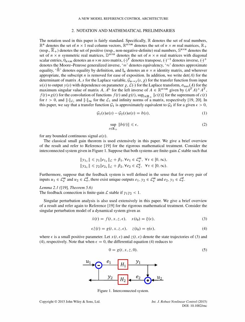
If isolated real roots ´ D hi .t; x/; i D 1; 2; : : : ; k exist, then the reduced system can be defined as

Px.t/ D f .t; x; h.t; x/; 0/; x.t0/ D �.�/: (6)

Let Nx.t/ denote the state trajectory of (6). Finally, the boundary layer model is given as

dy

d�D g.t0; �0; y C h.t0; �0/; 0/; y.0/ D �.0/ � h.t0; �0/; (7)

dy

d�D g.t; x; y C h.t; x/; 0/; y.0/ D �.0/ � h.t0; �0/; (8)

where � D t=�.

Lemma 2.2 ([19], Theorem 11.1)Consider the singular perturbation problem of (3) and (4), and let ´ D h.t; x/ be an isolated root of(5). Assume that the following conditions are satisfied for all Œt; x; ´ � h.t; x/; � 2 Œ0; t1 �Dx �Dy � Œ0; �0 for some domains Dx � Rn and Dy � Rm, in which Dx is convex and Dy containsthe origin.

The functions f and g, their first partial derivatives with respect to .x; ´; �/, and the firstpartial derivative of g with respect to t are continuous. The function h.t; x/ and the JacobianŒ@g.t; x; ´; 0/=@´ have continuous first partial derivatives with respect to their arguments. Theinitial data �.�/ and �.�/ are smooth functions of �. The reduced problem (6) has a unique solution Nx.t/ 2 S, for t 2 Œt0; t1 with S as a compact

subset of Dx . The origin is an exponentially stable equilibrium point of the boundary layer model (8), uni-

formly in .t; x/. Let Ry � Dy be the region of attraction of (7) andy be a compact subset ofRy .

Then, there exists a positive constant �? such that for all �0�h.t0; �0/ 2 y and 0 < � < �?, thesingular perturbation problem of (3) and (4) has a unique solution x.t; �/; ´.t; �/ on Œt0; t1, and

x.t; �/ � Nx.t/ D O.�/; (9)

´.t; �/ � h.t; Nx.t// � Oy.t=�/ D O.�/ (10)

hold uniformly for t 2 Œt0; t1, where Oy.�/ is the solution of the boundary layer model (5).

3. PROBLEM FORMULATION

Consider a class of uncertain dynamical systems given by

Px.t/ D Ax.t/C BŒƒu.t/C �.x; t/; x.0/ D x0; t 2 RC; (11)

where x.t/ 2 Rn is the state vector available for feedback, u.t/ 2 Rm is the control input restrictedto the class of admissible controls consisting of measurable functions, A 2 Rn�n and B 2 Rn�m

are the known system matrices such that the pair .A;B/ is controllable and det.BTB/ ¤ 0,ƒ 2 Rm�mC \ Dm�m is an unknown control effectiveness matrix, and � W Rn � NRC ! Rm is acontinuously differentiable function representing system uncertainty.

Assumption 3.1The set of possible uncertainty in (11) is given as

�.�; �/ 2 ˆ ,®� W Rn � NRC ! Rm W �.0; �/ D 0; �T .x; t/�.x; t/ 6 w?xT x; x 2 Rn; t 2 NRC

¯;

where w? 2 RC is a known (conservative) bound [21]. Equivalently, the set of possible uncertaintycan be given as



�.�; �/ 2 ˆ ,®� W D � NRC ! Rm W �.0; �/ D 0; �T .x; t/�.x; t/ 6 w?xT x; x 2 D; t 2 NRC

¯;

where D Rn is a known set of possible system states.

Assumption 3.2The unknown control effectiveness matrixƒ 2 Rm�mC \Dm�m satisfiesƒ?L 6 kƒk1 6 ƒ?U, whereƒ?L; ƒ

?U 2 RC are known (possibly conservative) bounds. The nominal case is recovered when

ƒ D Im.

Next, consider the reference system given by

Pxr.t/ D Arxr.t/C Brc.t/; xr.0/ D xr0; t 2 RC; (12)

where xr.t/ 2 Rn is the reference state vector.

c.t/ , cd.t/C cg.t/; (13)

where cd.t/ 2 Rm is a bounded continuously differentiable tracking command (or cd.t/ � 0 forstabilization), cg.t/ 2 Rm is the command governor signal to be defined later, Ar 2 Rn�n is theHurwitz reference system matrix, and Br 2 Rn�m is the reference command input matrix. We willalso consider an ideal reference system given as

Pxr.t/ D Arxr.t/C Brcd.t/; xr.0/ D xr0; t 2 RC (14)

that captures a desired closed-loop dynamical system response.

Remark 3.1In the standard model reference (adaptive) control formulation [5–7], there is no distinction betweenthe two reference systems (12) and (14) because, in that case, the command governor signal cg.t/in (13) is equivalently zero. The model reference formulation presented here is different because,as shown later in Theorem 5.1, it is possible for the uncertain system to track the ideal referencesystem (14) in both transient time and steady state by using a control formulation that utilizes thereference system (12).

Let the feedback control law be given by

u.t/ D K1x.t/CK2c.t/; (15)

where K1 2 Rm�n and K2 2 Rm�m are the feedback and feed forward gains, respectively, suchthat Ar D AC BK1, Br D BK2, and det.K2/ ¤ 0 hold.

Next, let the command governor signal be

cg.t/ , G�.t/; (16)

where G 2 Rm�n is the matrix defined by

G , K�12 BL D K�12�BTB

��1BT ; (17)

and �.t/ 2 Rn is the command governor output generated by

P�.t/ D ��.t/C �e.t/; �.0/ D 0; t 2 RC; (18)

�.t/ D ��.t/C .Ar � �In/e.t/; (19)

where �.t/ 2 Rn is the command governor state vector and � 2 RC is the command governor rate.Using (15) in (11) yields

Px.t/ D Ax.t/C Bƒu.t/C B�.x; t/

D Ax.t/C BŒu.t/ � u.t/C Bƒu.t/C B�.x; t/

D Arx.t/C Brcd.t/C Brcg.t/C BŒƒ � Iu.t/C B�.x; t/;

(20)



and the system error dynamics are given by using e.t/ , x.t/ � xr.t/, (12) and (20) as

Pe.t/ D Are.t/C BŒƒ � Iu.t/C B�.x; t/; e.0/ D e0; t 2 RC; (21)

where e0 , x0 � xr0.

Remark 3.2The goal of the proposed model reference controller is for the uncertain dynamical system (20) totrack the response of the ideal reference system (14) in both transient time and steady state. If thecommand governor signal, cg.t/, can suppress the effect of system uncertainty (ƒ and �.�; �/), then,as seen in (20), the system will indeed track the ideal reference system.

Remark 3.3The presented architecture borrows ideas from the adaptive control architecture presented in Refer-ence [2]. As shown in this section, the proposed architecture retains the uncertain system’s linearity,whereas the adaptive control architecture causes the system to become nonlinear. Therefore, in thiscase, established tools from linear systems theory can be used to analyze the resultant system andachieve predictable closed-loop performance.

4. STABILITY ANALYSIS

This section formulates the problem in a robust analysis framework to provide conditions for closed-loop system stability. For this purpose, we define the following augmented dynamical system using(12), (16), and (20) as

P .t/ D QF .�/ .t/C QGı.t/C QJ cd.t/; .0/ D 0; t 2 RC; (22)

y.t/ D QH.�/ .t/ D Œx.t/; Nu.t/T ; (23)

ı.t/ D Œƒ � Iu.t/C �.x; t/; (24)

where .t/ 2 R3n is the augmented system state, QF .�/ 2 R3n�3n is the augmented systemmatrix, QG 2 R3n�m is the augmented uncertainty input matrix, QJ 2 R3n�m is the augmentedtracking command input matrix, y.t/ 2 R2n is the system output, and QH 2 R2n�3n is theaugmented system output matrix. Furthermore, .t/ D Œx.t/; xr.t/; �.t/

T , QG D ŒBT ; 0m�2nT ,

QJ D ŒBTr ; BTr ; 0m�n

T , and Nu.t/ D u.t/ �K2cd.t/,

QH.�/ D

�In 0n�n 0n�n

BL NAr CK1 �BL NAr �B

L

�; (25)

Figure 2. Augmented dynamical system in a robust analysis framework.



QF .�/ D

24Ar C BrG NAr �BrG NAr �BrG

BrG NAr Ar � BrG NAr �BrG

�In ��In ��In

35 ; (26)

and NAr D Ar��In. A block diagram showing the augmented dynamical system is given in Figure 2.Asymptotic stability of the upper block of the system when there is no uncertainty (i.e., ƒ � I

and �.�; �/ � 0) must be shown before small gain stability analysis of the uncertain system can beperformed. For this reason, we present the following lemma.

Lemma 4.1Let ƒ � I; �.�; �/ � 0, and cd .�/ � 0, then the augmented dynamical system given by (22) isasymptotically stable.

ProofTo show asymptotic stability, the system error e.t/, without any system uncertainty, is given asPe.t/ D Are.t/.

Now, define the following system by using (18) as

�Pe.t/P�.t/

�D OA

�e.t/

�.t/

�;

�e.0/

�.0/

�D

�e0�0

�; t 2 RC; (27)

where

OA ,�Ar 0

�In ��In

�: (28)

Note that OA is Hurwitz (because Ar is Hurwitz by definition and ��In is Hurwitz), and hence,�.t/ ! 0 and e.t/ ! 0 as t ! 1. As a direct consequence, �.t/ ! 0 and cg.t/ ! 0 as t ! 1and x.t/! 0 and xr.t/!0 as t !1. �

Remark 4.1The upper block of the system is a bounded-input bounded-output (BIBO) system when ƒ � I and�.�; �/ � 0 if cd .�/ 6� 0 because cd .t/ is bounded by definition.

Remark 4.2The upper block of the system with ƒ � I and �.�; �/ � 0 is asymptotically stable forany � > 0. However, in the following sections, it is shown that the closed-loop system per-formance is dependent on the selection of the command governor rate, �, when uncertaintiesare present.

Figure 3. Augmented system represented as interconnected transfer functions blocks.



Conditions for stability are now derived using L1 small gain analysis [19]. For clarity of exposi-tion and to highlight key features of the proposed framework, the case when ƒ � I and �.�; �/ 6� 0will first be considered. Second, its counterpartsƒ 6� I and �.x; t/ � 0will then be considered. Themain result of the paper considers the general case when ƒ 6� I and �.�; �/ 6� 0. Figure 3 illustratesthe system as a set of interconnected transfer function blocks.

4.1. Stability conditions for ƒ � I and �.�; �/ 6� 0

In this section, conditions for closed-loop stability when ƒ � I and �.�; �/ 6� 0 are presented usingL1 small gain analysis. The following result is needed for our analysis.

Lemma 4.2Consider a transfer function defined by

G.s; �/ D�

�s

s C �In � A

�.sIn � A/

�1; (29)

where A is Hurwitz and let a.s/ and b.s/ be bounded continuous signals. If G.s; �/a.s/ D b.s/,then a.t/ C �.t; �/ D b.t/, where �.t; �/ is a bounded function and �.t; �/ � 0 and b.t/ � a.t/

when � is sufficiently large and t 2 RC.

ProofFirst, �.t; �/ is a bounded function because a.t/ and b.t/ are bounded by definition. Next, to provethat �.t; �/ � 0 for sufficiently large �, first rewrite the transfer function as

G.s; �/ D �

s C �s.sIn � A/

�1 � A.sIn � A/�1: (30)

Now take the inverse Laplace transform

L�1.G.s; �// D �e��t ��AeAt C 1

�� AeAt

D �e��tZ t

0

�e��

�AeA� C 1

�d� � AeAt

D �e��tZ t

0

Ae.AC�/� C e�� d� � AeAt

D �e��t

"A.AC �In/

�1�e.AC�/t � 1

Ce�t � 1

�

#� AeAt

D A�.AC �In/�1�eAt � e��t

� e��t � AeAt C 1:

Note that e��t � 0, �.A C �In/�1 � In for sufficiently large �, and t 2 RC; thus,L�1.G.s; �// � 1 for sufficiently large �, where approximate equivalence for transfer functions isgiven by Equations (1) and (2). Finally, it can be seen that

�.t; �/ DhA� .AC �In/

�1�eAt � e��t

� e��t � AeAt

i� a.t/ (31)

and �.t; �/ � 0 for sufficiently large � and t 2 RC. �We now consider stability conditions for ƒ � I and �.�; �/ 6� 0. Before we present the stability

conditions, Figure 3 is used to define the closed-loop transfer function from the system uncertaintyı.s/ to the system state x.s/ as

QGı!x.s; �/ D Gı!x.s/C Gc!x.s/GGe!�.s; �/Gı!x.s/: (32)

Lemma 4.3Consider the uncertain dynamical system given by (22)–(24) subject to Assumption 3.1 and ƒ � I.If k QGı!x.s; �?/kL1w? < 1, then the system is BIBO stable when � D �?.



ProofThe stability of the upper block in Figure 1 is given by Lemma 4.1. The L1 small gain theorem isnow used to conclude the proof [19]. �

The following results show that there always exists a �? such that k QGı!x.s; �?/kL1w? < 1 forall �.�; �/ 2 ˆ.

Lemma 4.4Consider the uncertain dynamical system given by (22)–(24) subject to Assumption 3.1 and ƒ � I.There always exists a �? such that k QGı!x.s; �?/kL1w? < 1.

ProofFirst, we solve for x.t/ from the closed-loop transfer function (32) as

x.t/ D L�1Gı!x.s/ı.s/C Gc!x.s/GGe!�.s; �/Gı!x.s/ı.s/

�: (33)

From (18) to (20), Ge!�.s; �/Gı!x.s/ can be written as

Ge!�.s; �/Gı!x.s/ D�

�s

s C �In � Ar

�.sIn � Ar/

�1B:

Using Lemma 4.2, for sufficiently large �, Ge!�.s; �/Gı!x.s/ � �B , where approximateequivalence for transfer functions is given by Equations (1) and (2). Thus,

x.t/ � L�1Œ.sIn � Ar/Bı.s/ � .sIn � Ar/BrGBı.s/

� L�1Œ.sIn � Ar/Bı.s/ � .sIn � Ar/Bı.s/ � 0:

As a result, k QGı!x.s; �/kL1 � 0 for sufficiently large �. �

Remark 4.3Closed-loop stability of the uncertain dynamical system is guaranteed by sufficiently increasing �when ƒ � I and �.�; �/ 6� 0 for any �.�; �/ 2 ˆ.

4.2. Stability conditions for ƒ 6� I and �.�; �/ � 0

Again, Figure 3 is used to define the closed-loop transfer function from ı.s/ to Nu.s/ as

Gı!Nu.s; �/ D K2GGı!�.s; �/CK1 QGı!x.s; �/: (34)

The transfer function Gı!�.s; �/ can be derived from Figure 3 as

Gı!�.s; �/ DGe!�.s; �/Gı!x.s/

Ge!�.s; �/.Gc!xr.s/G � Gc!x.s/G/C I:

Note that Gc!xr.s/ D Gc!x.s/, thus, the transfer function is reduced to

Gı!�.s; �/ D�.s/

ı.s/D Ge!�.s; �/Gı!x.s/: (35)

Recall that for sufficiently large �, Ge!�.s; �/Gı!x.s/ � �B and QGı!x.s; �/ � 0. Thus,

Gı!Nu.s; �/ � �K2GB D �I (36)

for sufficiently large �, where approximate equivalence for transfer functions is given byEquations (1) and (2).

Lemma 4.5Consider the uncertain dynamical system given by (22)–(24) subject to Assumption 3.2 and �.�; �/ �0. If kGı!Nu.s; �?/kL1kƒ � Ik1 < 1, then the system is BIBO stable when � D �?.



ProofThe stability of the upper block in Figure 1 is given by Lemma 4.1. The L1 small gain theorem isnow used to conclude the proof [19]. �

Remark 4.4Bounds for allowable ƒ can be trivially computed because it was shown for sufficiently large �that Gı!Nu.s; �/ � �I. Thus, kƒ � Ik1 < 1. Note the case when ƒ D 0 does not satisfy thisrequirement. This is expected because this corresponds to a case when all of the system’s actuatorsare not working. By simple extension of this argument, ifƒ D 2I, then the inequality is not satisfied.

Remark 4.5It may be possible for the uncertain dynamical system to remain stable even if ƒ D 2I, but theanalysis presented here will not be able to capture this because of the symmetry of the smallgain theorem.

4.3. Stability conditions for ƒ 6� I and �.x; t/ 6� 0

The following result now considers the general case where ƒ 6� I and �.x; t/ 6� 0. Beforepresenting this result, we will define the following:

"1.t/ D Œcd.t/; ı.t/T ; (37)

"2.t/ D y.t/C0n�1; .K2cd.t//

T�T; (38)

where y.t/ D Œx.t/; u.t/�K2cd .t/T . Figure 4 illustrates the uncertain dynamical system makinguse of (37) and (38).

Theorem 4.1Consider the uncertain dynamical system given by (22)–(24) subject to Assumptions 3.1 and 3.2,ƒ 6� I and �.x; t/ 6� 0. If kGı!Nu.s; �?/kL1kƒ� Ik1Ck QGı!x.s; �?/kL1w? < 1, then the systemis BIBO stable when � D �?.

ProofFrom (12) and (20), note that

kGcd!x.s; �?/kL1 D kGcd!xr.s; �

?/kL1 <1: (39)

Also, using Figure 3,

Gcd!Nu.s; �?/ D K1Gcd!x.s; �

?/CK2GGe!�.s; �?/ŒGcd!x.s; �?/ � Gcd!xr.s; �

?/;

Gcd!Nu.s; �?/ D K1Gcd!x.s; �

?/:(40)

Thus,

kGcd!Nu.s; �?/kL1 D kK1Gcd!x.s; �

?/kL1 <1: (41)

Figure 4. Uncertain dynamical system in a robust analysis framework.



Next, by using (37), an upper bound for "1.t/ is given as

k"1.t/kL1 6 kcd.t/kL1 C kı.t/kL16 .1C kƒ � Ik1/kcd.t/kL1 C kƒ � Ik1k Nu.t/kL1 C w

?kx.t/kL16 .1C kƒ � Ik1/kcd.t/kL1 C kƒ � Ik1kGcd!Nu.s; �

?/kL1kcd.t/kL1C kƒ � Ik1kGı!Nu.s; �?/kL1k"1.t/kL1 C w?kGcd!x.s; �

?/kL1kcd.t/kL1C w?kGı!x.s; �?/kL1k"1.t/kL1 :

(42)

Define N� D kƒ � Ik1kGı!Nu.s; �?/kL1 C w?kGı!x.s; �?/kL1 for easy of exposition. BecauseN� < 1,

k"1.t/kL1 61

1 � N�.1Ckƒ�Ik1Ckƒ�Ik1kGcd!Nu.s; �

?/kL1Cw?kGcd!x.s; �

?/kL1/kcd.t/kL1

for all t 2 RC. An upper bound for y.t/ can now be given as

ky.t/kL1 6 kx.t/kL1 C ku.t/kL16 kGcd!Nu.s; �

?/kL1kcd.t/kL1 C kGı!Nu.s; �?/kL1k"1.t/kL1C kGcd!x.s; �

?/kL1kcd.t/kL1 C kGı!x.s; �?/kL1k"1.t/kL1

for all t 2 RC. �

Remark 4.6Let GY!X .s/ , X.s/=Y.s/ D C.sIn � A/

�1B . Then, an upper bound for the L1 system norm isgiven by Chellaboina et al. [20]

kGY!XkL1 61p˛�1=2max

�CQ˛C

T�; (43)

where Q˛ 2 Rn�n

C \ Sn�n being the unique solution to the Lyapunov equation 0 D ArQ˛ C

Q˛ArT C ˛Q˛ C BrBr

T , with ˛ 2 RC be such that Ar C˛2In is Hurwitz.

Remark 4.7The resultant system’s gain and phase margins will, in general, depend on the command governorrate, �. If given predefined requirements on the stability margins of the system, possible values of� can be computed. Therefore, in this case, the amount of system uncertainty, characterized by w?,ƒ?L, and ƒ?U, that can be mitigated will be reduced. However, the designer may choose to relaxrequirements on stability margins if a larger set of uncertainties can be mitigated.

5. PERFORMANCE ANALYSIS

In the previous section, conditions for stability were derived. Even though stability is important,overall transient time and steady-state system performance is also of practical interest. In thissection, we show that transient and steady-state performance is improved as � is increased. The fol-lowing theorem shows that the controlled uncertain dynamical system (11) approximates the idealreference system (14) for sufficiently large �.

Theorem 5.1Consider the uncertain dynamical system given by (11) subject to Assumptions 3.1 and 3.2, thereference system given by (12), the feedback control law given by (15), and the command governorgiven by (16)–(19). Then there exists �? such that if � > �?, then x.t/ � ´.t/ D O.1=�/, where´.t/ evolves according to

P.t/ D Ar´.t/C Brcd.t/; ´.t0/ D x0 (44)

for all initial conditions .x0; e0; �0/ 2 Rn �Rn �Rn.



ProofThe proof is a direct application of Lemma 2.2. We first note that the command governor dynamicalsystem given by (18) and (19) can be written in Laplace domain as

Ge!�.s/ D Ar �s

1�s C 1

In; (45)

and therefore,

� P�.t/ D ��.t/C �Ar Pe.t/C Are.t/ � Pe.t/; (46)

where � D 1=�. Next, consider the following singular perturbation model

Px.t/ D Arx.t/C Brcd.t/C Brcg.t/C BŒƒ � Iu.t/C B�.x; t/; x.0/ D x0; t 2 RC; (47)

Pe.t/ D Are.t/C BŒƒ � Iu.t/C B�.x; t/; e.0/ D e0; (48)

� P�.t/ D ��.t/C �Ar Pe.t/C Are.t/ � Pe.t/; �.0/ D .Ar � �In/e0: (49)

Note that when � D 0, then the isolated root �.t/ D Are.t/� Pe.t/ can be derived from (49) and thereduced system can be defined as

Px.t/ D Arx.t/C Brcd.t/; (50)

Pe.t/ D Are.t/ � �.t/; (51)

and the boundary layer model is given as

dy

d�D �y.�/; y.0/ D �.t0/ � Are.t0/C Pe.t0/: (52)

Note that because cd.t/ and �.x; t/ are assumed to be continuously differentiable and the singularperturbation model is linear, the partial derivatives of the dynamical functions and the reduced modelare continuous. Furthermore, all initial conditions are smooth functions of �. The reduced systems(50) and (51) have a unique solution. Finally, the boundary layer model is globally exponentiallystable, and therefore, y 2 Rn. Therefore, x.t/ � ´.t/ D O.�/ when � < 1=�? for all initialconditions .x0; e0; �0/ 2 Rn �Rn �Rn. �

Remark 5.1It has been shown that for a sufficiently large command governor rate �, the system is stable for anybounded uncertainty and behaves like the ideal reference system (44). However, for real physicalsystems, a very high command governor rate can amplify noise that possibly exists in the statemeasurement due to Equation (45). The following section will present a modification to the proposedcommand governor to make its output less sensitive to high frequency signal content.

6. ROBUST MODEL REFERENCE CONTROL

It was shown in Theorem 5.1 that for a large command governor rate, �, the uncertain dynam-ical system (11) approximates the ideal reference system (44). Still, as noted in Remark 5.1, alarge command governor rate may lead to measurement noise amplification. This section presentsa modification to the command governor such that its output �.t/ is less sensitive to the high fre-quency content (such as measurement noise) when a large command governor rate is chosen. Forthis purpose, let the modified command c.t/ be given as

c.t/ D cd.t/CG�f.t/; (53)



where G�f.t/ is the modified command governor signal with G 2 Rm�n being the matrix definedby (17) and �f.t/ 2 Rn being the modified command governor output generated by

P�f.t/ D ��f.t/C �ef.t/; �f.0/ D 0; t 2 RC; (54)

�f.t/ D ��f.t/C .Ar � �In/ef.t/; (55)

where �f.t/2Rn is the command governor state vector, �2RC is the command governor rate, andef.t/ is generated by

Pef.t/ D �ˇef.t/C ˇe.t/; ef.0/ D e.0/; t 2 NRC; (56)

where ˇ 2 RC.

Remark 6.1The filter described by (56) is a simple example of a possible low-pass filter. More elaborate filterarchitectures can be selected to serve the same purpose. That is, the filter selection is not unique.Nevertheless, as shown later, filter selection changes the set of allowable ƒ and �.�; �/ and over-all transient time and steady-state system performance. The following analysis assumes the filterarchitecture as presented in (56). However, other architectures can easily be analyzed similarly.

The augmented system state vector can be modified to include the modified command governorstate and error as

m.t/ D Œx.t/; xr.t/; ef.t/; �f.t/T 2 R4n: (57)

The system matrices are now defined as QGm D ŒBT ; 0m�3n

T , QJm D ŒBTr ; B

Tr ; 0m�2n

T ,

QHm.�/ D

�In 0n�n 0n�n 0n�nK1 0n�n B

L NAr �BL

�; (58)

QFm.�/ D

2664Ar 0n�n BrG NAr �BrG

0n�n Ar BrG NAr �BrG

ˇIn �ˇIn �ˇIn 0n�n0n�n 0n�n �In ��In

3775 ; (59)

and NAr D Ar � �In. To prove that the upper block of the modified system, as given in Figure 2, isstill asymptotically stable when there is no uncertainty, the following lemma is presented.

Lemma 6.1Let ƒ � I; �.�; �/ � 0, and cd .�/ � 0, then the modified augmented dynamical system given by(22), .t/ D m.t/, QF .�/ D QFm.�/; QG D QGm, and QJ D QJm is asymptotically stable.

ProofTo show stability asymptotically, the system error e.t/, without any system uncertainty, is given asPe.t/ D Are.t/. Now define the following system by using (54) and (56) as2

4 Pe.t/Pef.t/P�f.t/

35 D OA

24e.t/ef.t/

�f.t/

35 ;

24e.0/ef.0/

�f.0/

35 D

24e0ef0

�f0

35 ; t 2 RC;

where

OA ,

24 Ar 0 0

ˇIn �ˇIn 0

0 �In ��In

35 : (60)



Note that OA is Hurwitz (because Ar is Hurwitz by definition, �ˇIn and ��In are Hurwitz), andhence, �.t/ ! 0; e.t/ ! 0, and ef.t/ ! 0 as t ! 1. As a direct consequence, �f.t/ ! 0 andcg.t/! 0 as t !1 and x.t/! 0 and xr.t/! 0 as t !1. �

Remark 6.2The system when ƒ � I and �.�; �/ � 0 is asymptotically stable for any ˇ, � > 0. Nevertheless, theclosed-loop system performance depends on the selection of ˇ and � in the presence of uncertainties.

The modified system can be represented by interconnected transfer function blocks as shown inFigure 5. The effect the modification has on the set of allowableƒ and �.�; �/ can be seen by solvingfor x.t/ from the closed-loop transfer function QGı!x.s; �/ as

x.t/ D L�1Gı!x.s/ı.s/C Gc!x.s/GGef!�f.s; �/Ge!ef.s; �/Gı!x.s/ı.s/

�D L�1

Gı!x.s/ı.s/C Gc!x.s/GGı!�f.s; �/ı.s/

�D L�1

�Gı!x.s/ı.s/C Gc!x.s/G

�Ar �

�s

s C �In

�ˇ

s C ˇIn.sIn � Ar/

�1Bı.s/

�

D L�1�Gı!x.s/ı.s/C Gc!x.s/G

�ˇ

s C ˇ

��s

s C �In � Ar

�.sIn � Ar/

�1Bı.s/

�:

For sufficiently large �,

x.t/ � L�1"Gı!x.s/ı.s/C Gc!x.s/GB

�1sˇC 1

ı.s/

#

� L�1".sIn � Ar/

�1Bı.s/ � .sIn � Ar/�1B

�1sˇC 1

ı.s/

#:

(61)

For illustrative purposes, assume that the filter given by (56) is an ideal filter such that

ı.j!/ D�1

j!ˇC 1

ı.j!/; ! 6 ˇ;

0 D�1

j!ˇC 1

ı.j!/; ! > ˇ:

Thus,

x.t/ � L�1.j!In � Ar/

�1Bı.j!/�; ! > ˇ: (62)

Figure 5. Modified augmented system represented as transfer functions.



In general, k QGı!x.s; �/kL1 6� 0 for sufficiently large �, and there does not exist a �? such thatk QGı!x.s; �?/kL1kw? < 1 for all w?. Thus, the set of allowable �.�; �/ is limited. The modifiedclosed-loop transfer function from the system uncertainty ı.s/ to the Nu.s/ is given as

Gı!Nu.s; �/ D K2GGı!�f.s; �/CK1QGı!x.s; �/: (63)

For sufficiently large �,

Gı!Nu.s; �/ D K2GB�1sˇC 1CK1

".sIn � Ar/

�1B � .sIn � Ar/�1B

�1sˇC 1

#

D�1sˇC 1CK1

".sIn � Ar/

�1B � .sIn � Ar/�1B

�1sˇC 1

#:

(64)

Thus, for sufficiently large �, kGı!Nu.s; �/kL1 > 1. The bounds of allowableƒ given in Remark 4.4for the case when ƒ ¤ I and �.�; �/ D 0 may no longer be valid.

Remark 6.3Note that k QGı!x.s; �/kL1 and kGı!Nu.s; �/kL1 , for sufficiently large �, are determined by ˇ, thereference system, and the system’s input matrix and not by the system’s uncertainty. Thus, the setof allowable ƒ and �.�; �/ can always be determined.

Remark 6.4Because the set of allowable ƒ and �.�; �/ can always be determined and is dependent on the ref-erence system, the reference system can be selected in order to accommodate a given set of ƒ and�.�; �/. Therefore, given a set of system uncertainty, an error filter, and the system’s input matrix, aset of allowable reference systems can be constructed.

Remark 6.5The filter deteriorates the command governor’s ability to suppress the system uncertainty signal,ı.t/, at high frequencies (filtered frequencies in the general case). Intuitively, the filter inhibits thecommand governor from receiving an accurate representation of the error and, thus, its ability tosuppress system uncertainty. Ideally, a filter should be selected such that noise is reduced whilemaintaining a sufficiently accurate representation of the error.

The following result is in order.

Theorem 6.1Consider the modified uncertain dynamical system given by (22)–(24), .t/ D m.t/, QF D QFm; QG DQGm, QH D QHm, and QJ D QJm subject to Assumptions 3.1 and 3.2, ƒ 6� I and �.x; t/ 6� 0. IfkGı!Nu.s; �?/kL1kƒ � Ik1 C k QGı!x.s; �?/kL1w? < 1, then the system is BIBO stable when� D �?.

ProofThis is a direct consequence of Theorem 4.1. �

Because the filter deteriorates the command governor ability to suppress the system uncertaintysignal, ı.t/, the uncertain dynamical system may not be able to approximate the ideal reference sys-tem as previously shown in Theorem 5.1. Still, as shown in the next result, the uncertain dynamicalsystem approximates the ideal reference system augmented with the difference between the filteredand unfiltered command governor outputs.

Lemma 6.2Consider the modified uncertain dynamical system given by (11) subject to Assumptions 3.1and 3.2, the reference system given by (12), the feedback control law given by (15) and (53),



and the command governor given by (54)–(55). Then there exists �? such that if � > �?, thenx.t/ � ´.t/ D O.1=�/, where ´.t/ evolves according to

P.t/ D Ar´.t/C Brcd.t/C BBL�f.t/ � �.t/; ´.t0/ D x0 (65)


ProofThe proof closely follows the arguments given to prove Theorem 5.1. As before, when 1=� D � D 0,then the isolated root is given as �.t/ D Are.t/ � Pe.t/ D �BŒƒ � Iu.t/ � B�.x; t/ and �f.t/ DAref.t/ � Pef.t/ and the reduced system can be defined as

Px.t/ D Arx.t/C Brcd.t/C BBL�f.t/ � �.t/; (66)

Pe.t/ D Are.t/ � �.t/; (67)

Pef.t/ D �ˇef.t/C ˇe.t/: (68)

Like the singularly perturbed system in Theorem 5.1, the system outlined here satisfies all of theconditions given in Lemma 2.2. Furthermore, y 2 Rn � Rn. Therefore, x.t/ � ´.t/ D O.1=�/

when 1=� < 1=�? for all initial conditions .x0; e0; �0/ 2 Rn �Rn �Rn. �

7. ACTUATOR DYNAMICS

While previously deriving stability conditions, we have neglected the effects of actuator dynam-ics on the system. The proposed command governor architecture suppresses the effects of systemuncertainty (ƒ and �.�; �/) by augmenting the input control signal with a command governor signal,cg.t/. As a result, an actuator’s input control signal may contain high frequency content outside ofthe operating bandwidth. Actuator dynamics may inhibit the command governor’s ability to sup-press the effects of system uncertainty due to actuator response time and bandwidth. In this section,we analyze the effects of actuator dynamics on the proposed model reference control architectureand discuss a modification to the framework to address this issue.

Consider a class of uncertain dynamical systems given by

Px.t/ D Ax.t/C BŒua.t/C �.x; t/; x.0/ D x0; t 2 RC; (69)

where x.t/ 2 Rn is the state vector available for feedback, ua.t/ 2 Rm represents the effectivecontrol input to the system, A 2 Rn�n and B 2 Rn�m are known system matrices such that thepair .A;B/ is controllable and det.BTB/ ¤ 0, and � W Rn � NRC ! Rm is the system uncertainty.Assumption 3.1 is assumed for this system as well. Furthermore, consider a class of dynamicalactuators represented by

Pua.t/ D ƒŒAaua.t/C Bau.t/; ua.0/ D ua0 ; t 2 RC; (70)

where u.t/ 2 Rm is the control input restricted to the class of admissible controls consisting ofmeasurable functions and given by (15), Aa 2 Rm�m and Ba 2 Rm�m are the system matricesrepresenting known actuator dynamics, andƒ 2 Rm�mC \Bm�m is an unknown control effectivenessmatrix such thatƒ?L 6 kƒk1 6 ƒ?U andƒ?L; ƒ

?U 2 R are known (conservative) bounds as discussed

in Assumption 3.2. Using the feedback control input (15), the uncertain dynamical system can bewritten as

Px.t/ D Arx.t/C BrŒcd.t/C cg.t/C BŒua.t/ � u.t/C �.x; t/; (71)

Px.t/ D Arx.t/C BrŒcd.t/C cg.t/C Bı.t/; (72)



and the system error dynamics are given as

Pe.t/ D Are.t/C BŒua.t/ � u.t/C �.x; t/ D Are.t/C Bı.t/: (73)

Note that ı.t/, as before, consists of �.�; �/ and the difference between the effective control inputand the computed control input. This suggests that the problem can be treated as before, and boundsfor allowable ƒ can be easily computed as in Remark 4.4. In Section 4, for the case where actu-ator dynamics are ignored, ƒ 6� I and �.x; t/ � 0, it was shown that Gı!Nu.s; �/ � �1 forsufficiently large �. It may seem that a simple extension of the analysis carried out in Remark 4.4can be performed to arrive at bounds for allowable ƒ when actuator dynamics are present. How-ever, this analysis leads to the condition that kGu!ua.s/ � IkL1 < 1 must hold for closed-loopstability. In physical implementations, actuators may be unresponsive for high frequency inputs(i.e., Gu!ua.s/ D 0 when s is large), and as a result, the condition will not be met. Notice thatunlike in Section 4, where the difference between the effective control input and the computed con-trol input was static (ƒ), when actuator dynamics are considered, the difference is dependent onfrequency (Gu!ua.s/).

In order to solve this problem, we propose a filter on the input of system (15) such that

Gu!uf.s/u.s/ D uf.s/: (74)

And the following condition holds

kŒGuf!uaf.s/ � IGu!uf.s/kL1 < 1; (75)

where Guf ! uaf.s/ represents the actuator dynamics given as

Puaf.t/ D ƒAaua f.t/C Bauf.t/

�; (76)

where uf 2 Rm is the filtered input, uaf.t/ filtered effective control input, and u.t/ is the controlinput given by Equation (15). Intuitively, the filter should be selected by considering the bandwidthof the actuator. By limiting the bandwidth of the control input, it is ensured that the differencebetween the filtered computed input and the filtered effective input is limited. Notice that the set ofallowable ƒ will be dependent on the input filter.

Remark 7.1The modification presented in the previous section is ignored in this section because it is assumedthat the input filter is sufficient to limit measurement noise amplification. Nevertheless, if a separatefilter is needed, similar analysis can be carried out very easily.

The class of uncertain dynamical systems (69) with an input filter (74) is given as

Px.t/ D Ax.t/C BŒuaf.t/C �.x; t/; (77)

and the reference system (12) with an input filter (74) is given as

Pxr.t/ D Axr.t/C Buf.t/: (78)

Finally, the error dynamics between the reference system and the uncertain system are

Pe.t/ D Ae.t/C BŒuaf.t/ � uf.t/C �.x; t/: (79)

Conditions for closed-loop stability can be derived following a similar procedure as carried out inSections 4 and 6. However, as seen before, results will diverge from results in Section 4 because theinput filter inhibits the command governor’s ability to suppress system uncertainty. The allowableset of ƒ and �.�; �/ will be dependent on the selection of the input filter.

Lemma 7.1Consider the modified linear uncertain dynamical system given by (77) subject to Assumption 3.1,the reference system given by (78), the feedback control law given by (15) and (74), the command



governor given by (18)–(19), actuator dynamics (76), and the input filter condition (75). Then thereexists �? such that if � > �?, then x.t/ � ´.t/ D O.1=�/, where ´.t/ evolves according to

P.t/ D Ar´.t/C Brcd.t/C BŒuf.t/ � u.t/; ´.t0/ D x0 (80)


ProofThe proof closely follows the arguments given to prove Theorem 5.1. First, note that the modifieduncertain dynamical system can be represented as

Px.t/ D Arx.t/C Brcd.t/C BBL�.t/C BŒuaf.t/ � u.t/C �.x; t/: (81)

As before, when 1=� D � D 0, then the isolated root is given as �.t/ D Are.t/ � Pe.t/ and thereduced system can be defined as

Px.t/ D Arx.t/C Brcd.t/C BŒuf.t/ � u.t/; (82)

Pe.t/ D Are.t/ � �.t/: (83)

Like the singularly perturbed system in Theorem 5.1 the system outlined here satisfies all of theconditions given in Lemma 2.2. Furthermore, y 2 Rn � Rn. Therefore, x.t/ � ´.t/ D O.1=�/

when 1=� < 1=�? for all initial conditions .x0; e0; �0/ 2 Rn �Rn �Rn. �

Remark 7.2Note that actuator dynamics do not affect the approximation directly. This observation leads to theconclusion that if no input filter is needed, the uncertain dynamical system approximates the idealreference system for sufficiently large �.

Remark 7.3Notice from (80) (and (65)) that the uncertain dynamical system approximates the ideal referencesystem augmented with the difference between the control input (command governor output) andthe filtered control input (filtered command governor output). This highlights the effect of modifyingthe system through signal filtering.

Remark 7.4It is important to stress that all of the results presented will be conservative because the smallgain analysis is conservative. Thus, actual conditions for closed-loop stability results may be lessrestrictive than conditions presented.

Remark 7.5The effect of time delay on the proposed model reference controller can be analyzed using methodsshown earlier. Time-delay effects can simply be incorporated into the actuator dynamics. By reduc-ing the bandwidth of the control input, the difference between the delayed effective control inputand the computed control input can be limited. Thus, input filter selection will depend not only onactuator bandwidth but also on the amount of desired allowable time delay.

8. ILLUSTRATIVE NUMERICAL EXAMPLES

8.1. Example 1

Consider a nonlinear uncertain dynamical system given as

�Px1.t/Px2.t/

�D

�0 1

0 0

� �x1.t/

x2.t/

�C

�0

1

�Œƒu.t/C �.x; t/;

�x1.0/

Px2.0/

�D

�0

0

�; t 2 RC;



where the unknown system uncertainty is given asƒ D 0:9 and �.x; t/ D 0:2.x21Cx22/C0:3x1x2.

The dynamical system is known to operate in D D ¹x 2 R2 W x1 2 .�8; 8/; x2 2 .�1:5; 1:5/º.The ideal reference system is selected such that the feedback control law (15) is given byK1 D Œ�0:2 � 0:8 and K2 D 1:1, and the tracking command is a unity step function(cd.t/ D 1; t > 0). Suppose that for this system, conservative estimates of the system uncertaintyare given as w? D 3 (actual bound is approximately 2.08), ƒ?L D 0:6, and ƒ?U D 1:4. For thisstudy, Ne.t/ refers to the error between the nonlinear uncertain dynamical system and the idealreference system (44). k QGı!x.s; �/kL1 was approximated by the method discussed in Remark 4.6,and kGı!�.s; �?/kL1 was computed directly from bode plot analysis.

Figure 6 shows k QGı!x.s; �/kL1 and kGı!u.s; �?/kL1 as functions of �. As shown in Section 4,kGı!x.s; �/kL1 ! 0 and kGı!u.s; �?/kL1 ! 1 as �!1.

Figure 7 shows the response of the ideal reference system and the nonlinear uncertain dynamicalsystem with no command governor architecture implemented. The nonlinear uncertain dynami-cal system is unstable. This simulation study shows that the proposed model reference control

Figure 6. k QGı!x.s; �/kL1 (solid line) and kGı!u.s; �/kL1 (dotted line) as functions of �. As predicted byLemma 4.4 and Remark 4.4, k QGı!x.s; �/kL1 ! 0 and kGı!u.s; �/kL1 ! 1 as �!1.

Figure 7. The ideal reference system and (unstable) nonlinear uncertain dynamical system responses.



architecture can be used to shape the uncertain dynamical system’s response to track the idealreference system.

Figure 6 shows that when � D 100, k QGı!x.s; �/kL1 � 0:08 and kGı!u.s; �?/kL1 � 1:02.Thus, kGı!Nu.s; �?/kL1kƒ� Ik1 C k QGı!x.s; �?/kL1w? � 1:02� 0:4C 0:08� 3 D 0:648. Thus,the closed-loop stability condition in Theorem 4.1 is satisfied. Figure 8 shows the response of the

Figure 8. System response and tracking error when � D 100.

Figure 9. System response and tracking error when � D 100 and the initial tracking error is non-zero.



uncertain dynamical system with the command governor implemented when � D 100. Note that arelatively small tracking error results. Furthermore, the input given by equation (15) is well behaved.Therefore, as predicted by Theorem 5.1, the uncertain dynamical system approximated the idealreference system when � was made sufficiently large. Figure 9 shows the response of the system

Figure 10. System response and tracking error when � D 5.

Figure 11. System response and tracking error in the presence of actuator dynamics when � D 15, and aninput filter Gu!uf.s/u.s/ D

25sC25

is used.



with a non-zero initial tracking error. Note that the tracking error decays and is nearly zero after theinitial transient phase.

Figure 6 shows that when � D 5, kGı!Nu.s; �?/kL1kƒ� Ik1Ck QGı!x.s; �?/kL1w? < 1:66. Theclosed-loop stability condition in Theorem 4.1 is not satisfied. Figure 10 shows the response of theuncertain dynamical system with the command governor implemented when � D 5. Even thoughthe stability condition is not met, relatively good tracking is shown. The displayed system perfor-mance supports our suggestion made throughout our analysis that the derived stability conditionsare conservative.

8.2. Example 2

Next, we augment the nonlinear uncertain dynamical system given in Section 8.1 with actuatordynamics given by

Pua.t/ D ƒŒ�5ua.t/C 5u.t/; ua.0/ D 0; t 2 RC: (84)

When � D 15, an input filter given by Gu!uf.s/u.s/ D25sC25

was used. It was calculated thatkŒGuf!uaf

.s/ � IGu!uf.s/kL1 � 0:85. Thus, kGı!Nu.s; �?/kL1kŒGuf!uaf.s/ � IGu!uf.s/kL1 C

k QGı!x.s; �?/kL1w? � 1:11 � 0:85 C 0:21 � 3 D 1:57. Figure 11 shows the system response.Even though stability conditions were not met, the uncertain dynamical system was able to trackthe ideal reference system well. Notice that the computed control signal becomes more oscilla-tory when compared with Figures (8) and (10). However, because of the input filter in place,this oscillatory behavior is not necessarily transported to the actuator. Figure 12 shows the sys-tem response when the available input bandwidth was further restricted by using an input filterdescribed by Gu!uf.s/u.s/ D

5sC5

. By comparing Figures 11 and 12, it is seen that tracking errorincreases when the available input bandwidth decreases. However, acceptable system performanceis still obtained in both cases despite the addition of an input filter and augmenting the system withactuator dynamics.

Figure 12. System response and tracking error in the presence of actuator dynamics when � D 15, and aninput filter Gu!uf.s/u.s/ D

5sC5

is used.



9. CONCLUSION

We presented a novel model reference control architecture that effectively suppresses system uncer-tainty through input augmentation of the uncertain dynamical and reference systems. Sufficientconditions for closed-loop stability were derived using a robust control framework and L1 smallgain analysis. The set of allowable system uncertainty was shown to be easily computable. In addi-tion to closed-loop stability, it was shown that the uncertain dynamical system achieves predictabletransient and steady-state performance by approximating an ideal reference system if the commandgovernor rate, �, is properly chosen. Modifications to the proposed architecture in the form of fil-ters were developed in order to address measurement noise and actuator dynamics. Future researchinvolves extensions to uncertain systems with limited state information and cyber-physical systemswith limited computational power and energy.

ACKNOWLEDGEMENTS

This work was supported by the University of Missouri Research Board and the National Institute ofStandards and Technology with grant no. 70NANB1OH013.

REFERENCES

1. Zhou K, Doyle JC, Glover K. Robust and Optimal Control. Prentice Hall: Englewood Cliffs, NJ, 1996.2. Yucelen T, Johnson E. A new command governor architecture for transient respons shaping. International Journal of

Adaptive Control and Signal Processing 2013; 27(12):1065–1085.3. Yucelen T, Haddad WM. A robust adaptive control architecture for disturbance rejection and uncertainty suppression

with L1 transient and steady-state performance guarantees. International Journal of Adaptive Control and SignalProcessing 2012; 26(11):1024–1055.

4. Haddad WM, How JP, Hall SR, Bernstein DS. Extensions of mixed-� bounds to monotonic and odd monotonicnonlinearities using absolute stability theory. International Journal of Control 1994; 60(5):905–951.

5. Astrom KJ, Wittenmark B. Adaptive Control. Addison-Wesley: Reading, MA, 1989.6. Ioannou PA, Sun J. Robust Adaptive Control. Prentice-Hall: Upper Saddle River, NJ, 1996.7. Narendra KS, Annaswamy AM. Stable Adaptive Systems. Englewood Cliffs: Upper Saddle River, NJ, 1989.8. Yucelen T, Calise AJ. Derivative-free model reference adaptive control. AIAA Journal of Guidance, Control and

Dynamics 2011; 34:933–950.9. Hovakimyan N, Cao C. L1 Adaptive Control Theory: Guaranteed Robustness with Fast Adaptation, Vol. 21. SIAM,

2010.10. Lavretsky E, Wise K. Robust and Adaptive Control: With Aerospace Applications. Springer, 2012.11. Nguyen N, Krishnakumar K, Boskovic J. An optimal control modification to model-reference adaptive control for

fast adaptation. In AIAA Guidance, Navigation and Control Conference, Honolulu, Hawaii, 2008.12. Anderson B. Failures of adaptive control theory and their resolution. Communications in Information and Systems

2005; 5:1–20.13. Ioannou P, Kokotovic P. Instability analysis and improvement of robustness of adaptive control. Automatica 1984;

120(15):583–594.14. Stepanyan V, Krishnakumar K. MRAC revisited: Guaranteed performance with reference model modification. In

American Control Conference. IEEE: Baltimore, Maryland, 2010; 93–98.15. Stepanyan V. Adaptive control with reference model modification. Journal of Guidance, Control, and Dynamics

2012; 35(4):1370–1374.16. Stepanyan V. M-MRAC for nonlinear systems with bounded disturbances. In IEEE Conference on Decision and

Control and European Control Conference. IEEE: Orlando, Florida, 2011; 5419–5424.17. Lavretsky E. Reference dynamics modification in adaptive controllers for improved transient performance. In AIAA

Guidance, Navigation, and Control Conference, 2011.18. Gibson TE, Annaswamy AM, Lavretsky E. Adaptive Systems with Closed-loop Reference Models: Stability,

Robustness and Transient Performance, arXiv preprint arXiv:1201.4897, 2012.19. Khalil HK. Nonlinear Systems. Prentice Hall: Upper Saddle River, NJ, 1996.20. Chellaboina V, Haddad WM, Bernstein DS, Wilson DA. Induced convolution operator norms of linear dynamical

systems. Mathematics of Control, Signals, and System 2000; 13:216–239.21. Haddad WM, Chellaboina V. Nonlinear Dynamical Systems and Control. A Lyapunov-based Approach. Princeton

University Press: Princeton, NJ, 2008.


Documents

A new model reference control architecture: stability ...lacis.eng.usf.edu/resources/RNC3416.pdf · DOI: 10.1002/rnc.3416 A new model reference control architecture: Stability, performance,