Embed Size (px)
Citation preview

A New Method of Normal ApproximationAuthor(s): Sourav ChatterjeeSource: The Annals of Probability, Vol. 36, No. 4 (Jul., 2008), pp. 1584-1610Published by: Institute of Mathematical StatisticsStable URL: http://www.jstor.org/stable/30242900 .
Accessed: 08/09/2013 02:10
Your use of the JSTOR archive indicates your acceptance of the Terms & Conditions of Use, available at .http://www.jstor.org/page/info/about/policies/terms.jsp
.JSTOR is a not-for-profit service that helps scholars, researchers, and students discover, use, and build upon a wide range ofcontent in a trusted digital archive. We use information technology and tools to increase productivity and facilitate new formsof scholarship. For more information about JSTOR, please contact [email protected].
.
Institute of Mathematical Statistics is collaborating with JSTOR to digitize, preserve and extend access to TheAnnals of Probability.
http://www.jstor.org
This content downloaded from 130.60.206.42 on Sun, 8 Sep 2013 02:10:20 AMAll use subject to JSTOR Terms and Conditions
The Annals of Probability 2008, Vol. 36, No. 4, 1584-1610 DOI: 10.1214/07-AOP370 a Institute of Mathematical Statistics, 2008
A NEW METHOD OF NORMAL APPROXIMATION'
BY SOURAV CHATTERJEE
University of California, Berkeley We introduce a new version of Stein's method that reduces a large class of
normal approximation problems to variance bounding exercises, thus making a connection between central limit theorems and concentration of measure. Unlike Skorokhod embeddings, the object whose variance must be bounded has an explicit formula that makes it possible to carry out the program more easily. As an application, we derive a general CLT for functions that are ob- tained as combinations of many local contributions, where the definition of "local" itself depends on the data. Several examples are given, including the solution to a nearest-neighbor CLT problem posed by P. Bickel.
1. Introduction. Central limit theorems for general nonadditive functions of independent random variables have been studied by various authors using a variety of techniques. Some examples are: (i) the method of Haj6k projections and some sophisticated extensions (e.g., [20, 38, 43]); (ii) Stein's method of normal approx- imation (references in Section 2); (iii) the big-blocks-small-blocks technique and its modem multidimensional versions (e.g. [2, 6]); (iv) the martingale approach and Skorokhod embeddings; (v) the method of moments. In this paper, we present a new approach that may go beyond the limitations of these existing techniques. The power of the method is demonstrated through several applications, mainly geometrical in nature, that are otherwise difficult. In the related article [10], we provide some applications to random matrices.
The paper is organized as follows. Section 2 contains a brief discussion of Stein's method and our main results (Theorems 2.2 and 2.5). Examples are worked out in Section 3. Proofs of the main theorems are in Section 4.
2. Results. Recall that the Kantorovich-Wasserstein distance between two probability measures A and v on the real line is defined as
W(t, v) := sup Ifhd -
fhdv :h Lipschitz, with IhilLip < I}.
Received November 2006; revised July 2007. 1Supported in part by NSF Grant DMS-07-07054 and a Sloan Research Fellowship in Mathemat-
ics. AMS 2000 subject classifications. 60F05, 60B 10, 60D05. Key words and phrases. Normal approximation, central limit theorem, Stein's method, nearest
neighbors, coverage processes, quadratic forms, occupancy problems. 1584
This content downloaded from 130.60.206.42 on Sun, 8 Sep 2013 02:10:20 AMAll use subject to JSTOR Terms and Conditions
A NEW METHOD OF NORMAL APPROXIMATION 1585
Convergence of measures in the Kantorovich-Wasserstein metric is stronger than weak convergence. Based on the Kantorovich-Wasserstein distance, we introduce the following measure of "distance to Gaussianity."
DEFINITION 2.1. Let W be a real-valued random variable with finite second moment. Let A be the law of (W - E(W))/N/Var(W) and let v be the standard Gaussian law. We define
3w := 'W(/t, v).
This is our preferred metric of normal approximation in this paper. Using the bounds on the Wasserstein distance, analogous results can be obtained for the Kol- mogorov distance via smoothing, but the rates will be suboptimal. This problem is very common in Stein's method; obtaining optimal rates for the Kolmogorov metric requires extra work and new ideas (see, e.g., [13]). Since our main focus is on convergence to normality and not so much on error bounds, we will not worry about this issue here.
2.1. Stein's method. A well-known computation via integration by parts shows that if Z - N(0, 1), then E(pa(Z)Z) = E(p'(Z)) for all absolutely con- tinuous aQ with
Elop'(Z)| < oc. Conversely, if W is a random variable satisfying
E(ap(W)W) = E(ap'(W)) for all Lipschitz yo, then W , N(0, 1). Consequently, if
W is such that E(ap(W)W) E(p'(W)) for all yp belonging to a large class of functions, then one can expect the distribution of W to be close to the N(0, 1) distribution.
This is the key idea behind Stein's method of normal approximation, introduced by Charles Stein in the seminal paper [40] and later developed in his book [41]. Precise error bounds can be obtained in various ways. We will reproduce one of Stein's results (Lemma 4.2) that gives a bound on the Kantorovich-Wasserstein distance to normality.
However, the problem begins at this point. Given a random variable W that may be a complicated function of many other variables, there is no general method for showing that E(ap(W)W) W E(yp'(W)). Several powerful techniques for car- rying out this step under special conditions are available in the literature on Stein's method (e.g., exchangeable pairs [41], diffusion generators [5], dependency graphs [4, 13, 36], size bias transforms [23], zero bias transforms [22], specialized procedures like [21, 34, 35] and recent developments [11, 12], to cite a few), but, somehow, they all require something "nice" to happen. It is rarely the case that something arbitrary (like the Levina-Bickel statistic [30], to be discussed later) becomes amenable to any of the existing versions of Stein's method.
This is the ground that we attempt to break in this paper. Given a random vari- able W that is an explicit but arbitrary function of a collection of independent
This content downloaded from 130.60.206.42 on Sun, 8 Sep 2013 02:10:20 AMAll use subject to JSTOR Terms and Conditions
1586 S. CHATTERJEE
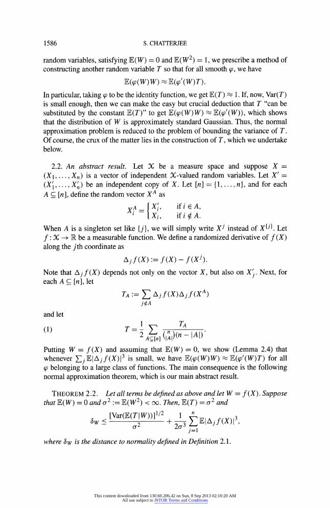
random variables, satisfying E(W) = 0 and E(W2) = 1, we prescribe a method of constructing another random variable T so that for all smooth y0, we have
E(p (W) W) E('(W) W)E(W)T). In particular, taking ap to be the identity function, we get E(T) ; 1. If, now, Var(T) is small enough, then we can make the easy but crucial deduction that T "can be substituted by the constant E(T)" to get E(ao(W)W) x E(p'(W)), which shows that the distribution of W is approximately standard Gaussian. Thus, the normal approximation problem is reduced to the problem of bounding the variance of T. Of course, the crux of the matter lies in the construction of T, which we undertake below.
2.2. An abstract result. Let X be a measure space and suppose X = (X1,..., Xn) is a vector of independent X-valued random variables. Let X' =
(XI, ..., XV) be an independent copy of X. Let [n] = {1, . . . , n}, and for each A C [n], define the random vector XA as
A Xi, if i E A, 1 Xi, if i/ A.
When A is a singleton set like {j}, we will simply write Xj instead of X{j}. Let f: X -- R be a measurable function. We define a randomized derivative of f(X) along the jth coordinate as
Aj f(X):= f(X) - f(xJ). Note that Ajf(X) depends not only on the vector X, but also on X'. Next, for each A C [n], let
TA 1 Aj f (X)AJ f(XA) jgA
1 TA 2 Ar[n] (A)(n - IA)
and let
(1)
Putting W = f(X) and assuming that E(W) = 0, we show (Lemma 2.4) that whenever j
jElAjf(X)13 is small, we have E(pa(W)W) E(0p'(W)T)
for all pa belonging to a large class of functions. The main consequence is the following normal approximation theorem, which is our main abstract result.
THEOREM 2.2. Let all terms be defined as above and let W = f(X). Suppose that E(W) = 0 and a2 := E(W2) < oo. Then, E(T) = U2 and
[Var(E(T I W))]1/2 1 Sw y 2 EIAjA f(X) I, j=l1
where 8w is the distance to normality defined in Definition 2.1.
This content downloaded from 130.60.206.42 on Sun, 8 Sep 2013 02:10:20 AMAll use subject to JSTOR Terms and Conditions
A NEW METHOD OF NORMAL APPROXIMATION 1587
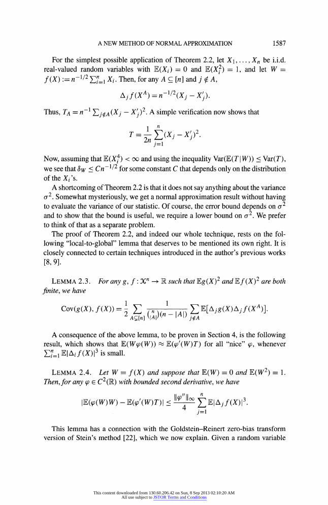
For the simplest possible application of Theorem 2.2, let X1,..., X, be i.i.d. real-valued random variables with E(Xi) = 0 and E(X2) = 1, and let W = f(X):= n-1/2 =1 Xi. Then, for any A C [n] and j 0 A,
Aj f(XA) = n-1/2(Xj - X).
Thus, TA = n-1 -
jOA(Xj - Xj
)2. A simple verification now shows that i
T = (Xj - X)>2 j=1
Now, assuming that E(X4) < oo and using the inequality Var(E(T I W)) < Var(T), we see that 8w < Cn-1/2 for some constant C that depends only on the distribution of the Xi's.
A shortcoming of Theorem 2.2 is that it does not say anything about the variance
a2. Somewhat mysteriously, we get a normal approximation result without having to evaluate the variance of our statistic. Of course, the error bound depends on a2 and to show that the bound is useful, we require a lower bound on a2. We prefer to think of that as a separate problem.
The proof of Theorem 2.2, and indeed our whole technique, rests on the fol- lowing "local-to-global" lemma that deserves to be mentioned its own right. It is closely connected to certain techniques introduced in the author's previous works [8, 9].
LEMMA 2.3. For any g, f: Xn -+ I~ such that Eg(X)2 and Ef(X)2 are both finite, we have
Cov(g(X), f(X)) =~- n
E[Ajg(X)Ajf(XA)]. Cov(g(X), ()(n -
IAI) A AC[n] |A j A A consequence of the above lemma, to be proven in Section 4, is the following
result, which shows that E(W'p(W)) ] E(ap'(W)T) for all "nice" yp, whenever E,1 El Ai f (X)13 is small.
LEMMA 2.4. Let W = f(X) and suppose that E(W) = 0 and E(W2) - 1. Then, for any Cp E C2 (R) with bounded second derivative, we have
IE(@p(W)W) - E(p'(W)T)I < IP4 IEAjf(X)o3 j=1
This lemma has a connection with the Goldstein-Reinert zero-bias transform version of Stein's method [22], which we now explain. Given a random variable
This content downloaded from 130.60.206.42 on Sun, 8 Sep 2013 02:10:20 AMAll use subject to JSTOR Terms and Conditions
1588 S. CHATTERJEE
W with mean zero and unit variance, a random variable W* is said to be a zero-bias transform of W if for all absolutely continuous op,
E(Wyo(W)) = E(p'(W*))
whenever both sides are well defined. It is shown in [22] that a zero-bias trans- form always exists and the closeness to normality for W can be measured by the closeness of the distributions of W and W* (which is usually done by construct- ing W* such that W ; W*). The problem with this approach, again, is that zero- bias transforms are hard to construct in general. Lemma 2.4 tells us that when- ever n EIEIAif(X)I3 is small, we have E(W y(W)) E(I'(W)E(TIW)). This means, roughly, that E(T I W) is approximately the Radon-Nikodym density of the law of W* with respect to the law of W, although such a density may not actually exist. Incidentally, such densities have been studied before, for example, in [7].
2.3. A general CLT for structures with local dependence. Numerous central limit theorems in probability theory have been conjectured or proven by follow- ing the intuition that a CLT for a sum of dependent summands should hold if "the dependencies are local in nature." Some notable examples are the classical big- blocks-small-blocks technique for analyzing m-dependent sequences, its multidi- mensional generalizations (e.g., [2, 6]), and the dependency graph method of [3]. Here, we provide a new method that is seemingly more powerful than the exist- ing techniques (our applications provide some evidence for this claim) and also gives explicit error bounds. The method is derived as a nontrivial corollary of The- orem 2.2.
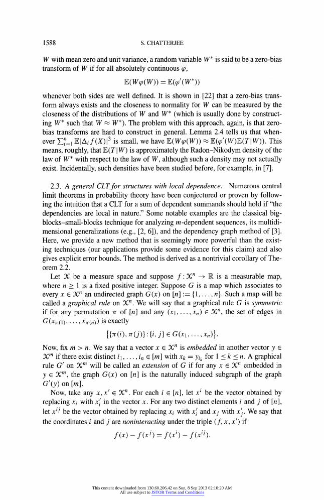
Let X be a measure space and suppose f: XVn -- R is a measurable map, where n > 1 is a fixed positive integer. Suppose G is a map which associates to every x E Xn an undirected graph G(x) on [n] := {1,..., n}. Such a map will be called a graphical rule on Xn. We will say that a graphical rule G is symmetric if for any permutation 7r of [n] and any (x1,..., xn) e Xn, the set of edges in G(xr(1),..., xr(n)) is exactly
{{1(i), 7r(j)}: {i, j} j G(xi,...,Xn)}. Now, fix m > n. We say that a vector x e Xn is embedded in another vector y E Xm if there exist distinct il, ..., in e [m] with xk = Yik for 1 < k < n. A graphical rule G' on Xm will be called an extension of G if for any x e Xn embedded in y e Xm, the graph G(x) on [n] is the naturally induced subgraph of the graph G'(y) on [m].
Now, take any x, x' e Xn. For each i E [n], let xi be the vector obtained by replacing xi with x' in the vector x. For any two distinct elements i and j of [n], let x'J be the vector obtained by replacing xi with x and with x. We say that the coordinates i and j are noninteracting under the triple (f, x, x') if
f(x) - f(xJ) = f(x') - f(x"J).
This content downloaded from 130.60.206.42 on Sun, 8 Sep 2013 02:10:20 AMAll use subject to JSTOR Terms and Conditions
A NEW METHOD OF NORMAL APPROXIMATION 1589
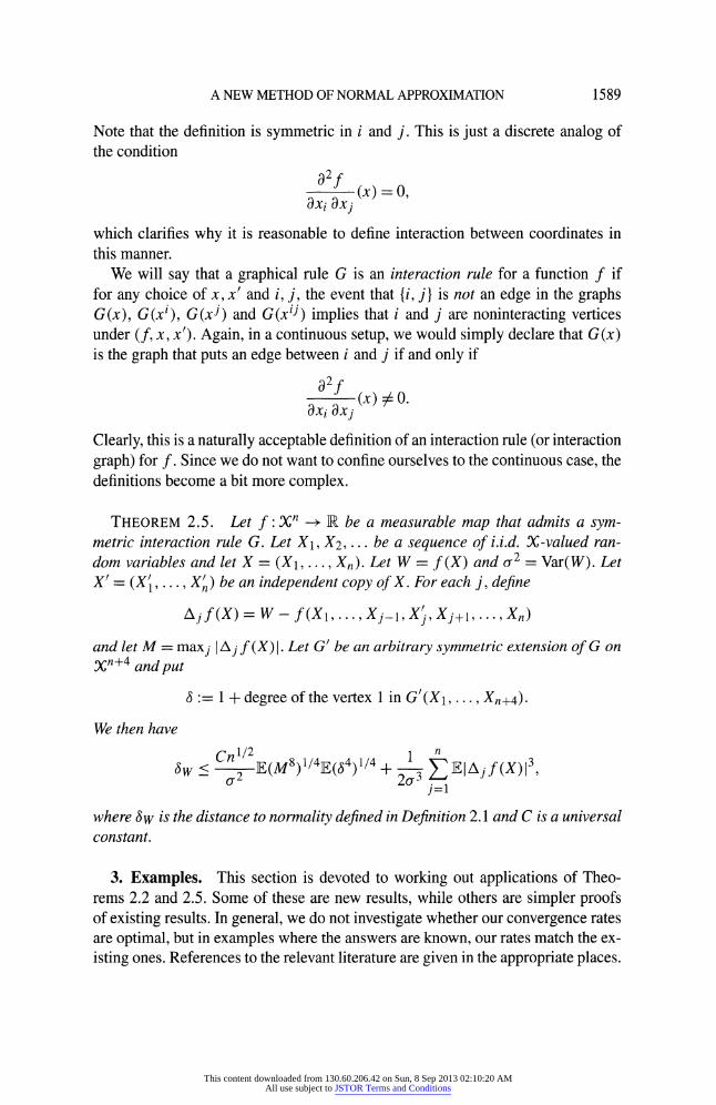
Note that the definition is symmetric in i and j. This is just a discrete analog of the condition
a2f (x) = 0,
8xi 8xj which clarifies why it is reasonable to define interaction between coordinates in this manner.
We will say that a graphical rule G is an interaction rule for a function f if for any choice of x, x' and i, j, the event that {i, j} is not an edge in the graphs G (x), G (x'), G (xj) and G (x'l) implies that i and j are noninteracting vertices under (f, x, x'). Again, in a continuous setup, we would simply declare that G(x) is the graph that puts an edge between i and j if and only if
a2f axi axj
Clearly, this is a naturally acceptable definition of an interaction rule (or interaction graph) for f. Since we do not want to confine ourselves to the continuous case, the definitions become a bit more complex.
THEOREM 2.5. Let f : Xn -+ IR be a measurable map that admits a sym- metric interaction rule G. Let X1, X2,... be a sequence of i.i.d. X-valued ran- dom variables and let X = (X1, ... , Xn). Let W = f (X) and a2 = Var(W). Let
X' = (X;, ..., X') be an independent copy of X. For each j, define
Aj f(X) = W - f(XI,..., Xj-_1, Xj, Xj+l,..., Xn)
and let M = maxj IAj f (X) I. Let G' be an arbitrary symmetric extension of G on Xn+4 and put
6 := 1 + degree of the vertex 1 in G'(X1, ..., Xn+4)
We then have
Cn1/2 1 E(M)14E(41/4 + w< E(M)/4E(Ajf(X)j
j=l
where 8w is the distance to normality defined in Definition 2.1 and C is a universal constant.
3. Examples. This section is devoted to working out applications of Theo- rems 2.2 and 2.5. Some of these are new results, while others are simpler proofs of existing results. In general, we do not investigate whether our convergence rates are optimal, but in examples where the answers are known, our rates match the ex- isting ones. References to the relevant literature are given in the appropriate places.
This content downloaded from 130.60.206.42 on Sun, 8 Sep 2013 02:10:20 AMAll use subject to JSTOR Terms and Conditions
1590 S. CHATTERJEE
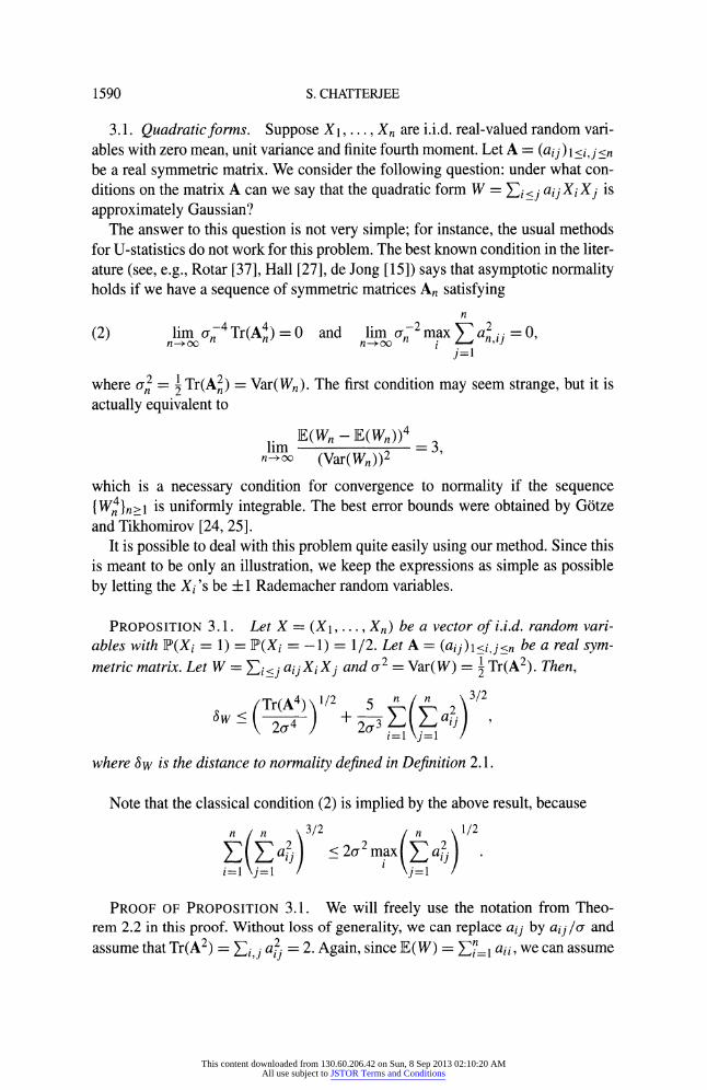
3.1. Quadratic forms. Suppose X1,..., X, are i.i.d. real-valued random vari- ables with zero mean, unit variance and finite fourth moment. Let A = (aij)l i,j <n be a real symmetric matrix. We consider the following question: under what con- ditions on the matrix A can we say that the quadratic form W = i <j aij Xi Xj is approximately Gaussian?
The answer to this question is not very simple; for instance, the usual methods for U-statistics do not work for this problem. The best known condition in the liter- ature (see, e.g., Rotar [37], Hall [27], de Jong [15]) says that asymptotic normality holds if we have a sequence of symmetric matrices An satisfying
n
(2) lim a-4 Tr(A4) = 0 and lim n-2
max E ,ij = 0, n-- 00 n--+ oc i j=1
where oa,2 = Tr(A2) = Var(Wn). The first condition may seem strange, but it is actually equivalent to
S E(Wn - E(Wn))4
lim = 3, n-o (Var(W,))2 which is a necessary condition for convergence to normality if the sequence
{Wn}n,>l is uniformly integrable. The best error bounds were obtained by Gdtze
and Tikhomirov [24, 25]. It is possible to deal with this problem quite easily using our method. Since this
is meant to be only an illustration, we keep the expressions as simple as possible by letting the Xi's be a 1 Rademacher random variables.
PROPOSITION 3.1. Let X = (X1,..., Xn) be a vector of i.i.d. random vari- ables with P](Xi = 1) = IP(Xi = -1) = 1/2. Let A = (aij)1<i,j<n be a real sym- metric matrix. Let W = Ej<j aijXi Xj and
a-2 = Var(W) = 1 Tr(A2). Then,
(Tr(A4)1/2 5 n n 3/2
i= 1 j
where 8w is the distance to normality defined in Definition 2.1.
Note that the classical condition (2) is implied by the above result, because
/ a02 < 2cr2
max aJ2
PROOF OF PROPOSITION 3.1. We will freely use the notation from Theo- rem 2.2 in this proof. Without loss of generality, we can replace aij by aij /o and assume that Tr(A2) = i,j aj = 2. Again, since E(W) = aii, we can assume
This content downloaded from 130.60.206.42 on Sun, 8 Sep 2013 02:10:20 AMAll use subject to JSTOR Terms and Conditions
A NEW METHOD OF NORMAL APPROXIMATION 1591
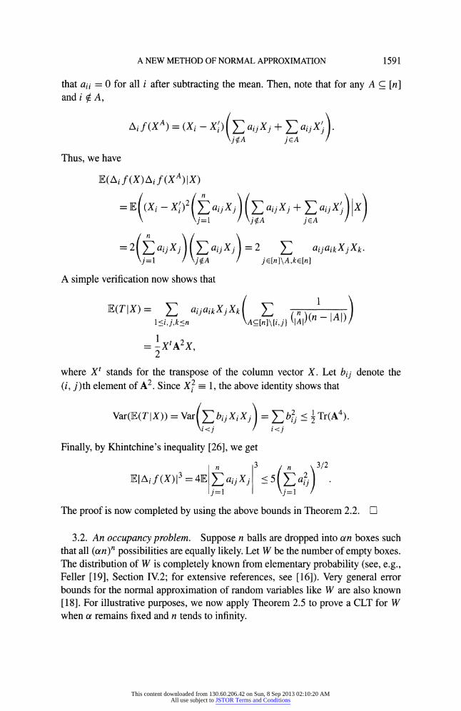
that aii = 0 for all i after subtracting the mean. Then, note that for any A C [n] and i A,
A, f (XA) = (Xi
- X)(
aijXj
+ aij) \jVA jEA
Thus, we have
E(Ai f (X)Ai f (XA)IX)
= E (Xi - X)2( aijXi aijXj + I aijX) X) (C (j=1 (jA jEA = 2 aijX J aijXj X 2 =
aijaikXjXk. jj=1jA jE[n]\A,kE[n]
A simple verification now shows that
E(TIX) = aijaikXjXk (L (j)(n-JAI)
1<i,j,k<n AC[n]\{i,j} A
= XtA2X, 2
where Xt stands for the transpose of the column vector X. Let bij denote the (i, j)th element of A2. Since
Xi2 - 1, the above identity shows that
Var(E(TIX)) = Var( bijXiXj) = b2 <Tr(A4). (i<<j i<j
Finally, by Khintchine's inequality [26], we get
El Aif(X)13 =4E aijXj < 5 a j= j=
The proof is now completed by using the above bounds in Theorem 2.2. O
3.2. An occupancy problem. Suppose n balls are dropped into an boxes such that all (an)n possibilities are equally likely. Let W be the number of empty boxes. The distribution of W is completely known from elementary probability (see, e.g., Feller [19], Section IV.2; for extensive references, see [16]). Very general error bounds for the normal approximation of random variables like W are also known [18]. For illustrative purposes, we now apply Theorem 2.5 to prove a CLT for W when a remains fixed and n tends to infinity.
This content downloaded from 130.60.206.42 on Sun, 8 Sep 2013 02:10:20 AMAll use subject to JSTOR Terms and Conditions
1592 S. CHATTERJEE
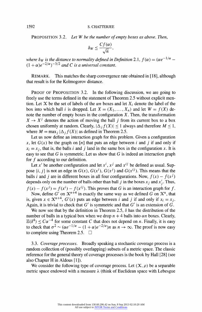
PROPOSITION 3.2. Let W be the number of empty boxes as above. Then,
Cf (a)
where 8w is the distance to normality defined in Definition 2.1, f (a) = (ae-1/a - (1 + a)e-2/a)-3/2 and C is a universal constant.
REMARK. This matches the sharp convergence rate obtained in [18], although that result is for the Kolmogorov distance.
PROOF OF PROPOSITION 3.2. In the following discussion, we are going to freely use the terms defined in the statement of Theorem 2.5 without explicit men- tion. Let X be the set of labels of the an boxes and let Xi denote the label of the box into which ball i is dropped. Let X = (X1, ..., Xn) and let W = f(X) de- note the number of empty boxes in the configuration X. Then, the transformation X --+ Xi denotes the action of moving the ball j from its current box to a box chosen uniformly at random. Clearly, IAj f(X)I < 1 always and therefore M < 1, where M = maxj IAj f(X)I as defined in Theorem 2.5.
Let us now define an interaction graph for this problem. Given a configuration x, let G(x) be the graph on [n] that puts an edge between i and j if and only if xi = xj, that is, the balls i and j land in the same box in the configuration x. It is easy to see that G is symmetric. Let us show that G is indeed an interaction graph for f according to our definition.
Let x' be another configuration and let xi, xJ and x'j be defined as usual. Sup- pose {i, j} is not an edge in G(x), G(x'), G(xJ) and G(x"J). This means that the balls i and j are in different boxes in all four configurations. Now, f(x) - f(xj) depends only on the number of balls other than ball j in the boxes xj and x'. Thus, f (x) - f (xJ) = f (x') - f (x'J). This proves that G is an interaction graph for f.
Now, define G' on Xn+4 in exactly the same way as we defined G on Xn, that is, given x e Xn+4, G'(x) puts an edge between i and j if and only if xi = xj. Again, it is trivial to check that G' is symmetric and that G' is an extension of G.
We now see that by the definition in Theorem 2.5, 8 has the distribution of the number of balls in a typical box when we drop n + 4 balls into an boxes. Clearly, E(84) < Ca-4 for some constant C that does not depend on n. Finally, it is easy to check that a2 a ( /e-1/a - (1 + a)e-2/a)n as n --+ o . The proof is now easy to complete using Theorem 2.5. O
3.3. Coverage processes. Broadly speaking a stochastic coverage process is a random collection of (possibly overlapping) subsets of a metric space. The classic reference for the general theory of coverage processes is the book by Hall [28] (see also Chapter H in Aldous [1]).
We consider the following type of coverage process. Let (X, p) be a separable metric space endowed with a measure k (think of Euclidean space with Lebesgue
This content downloaded from 130.60.206.42 on Sun, 8 Sep 2013 02:10:20 AMAll use subject to JSTOR Terms and Conditions
A NEW METHOD OF NORMAL APPROXIMATION 1593
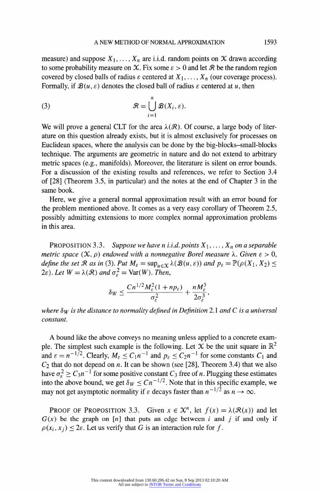
measure) and suppose X1, ..., Xn are i.i.d. random points on X drawn according to some probability measure on X. Fix some e > 0 and let R be the random region covered by closed balls of radius e centered at X1, ..., X, (our coverage process). Formally, if S (u, e) denotes the closed ball of radius e centered at u, then
n
(3) =US X,>. i=1
We will prove a general CLT for the area (?). Of course, a large body of liter- ature on this question already exists, but it is almost exclusively for processes on Euclidean spaces, where the analysis can be done by the big-blocks-small-blocks technique. The arguments are geometric in nature and do not extend to arbitrary metric spaces (e.g., manifolds). Moreover, the literature is silent on error bounds. For a discussion of the existing results and references, we refer to Section 3.4 of [28] (Theorem 3.5, in particular) and the notes at the end of Chapter 3 in the same book.
Here, we give a general normal approximation result with an error bound for the problem mentioned above. It comes as a very easy corollary of Theorem 2.5, possibly admitting extensions to more complex normal approximation problems in this area.
PROPOSITION 3.3. Suppose we have n i.i.d. points X1, ... , Xn on a separable metric space (X, p) endowed with a nonnegative Borel measure X.. Given 8 > 0, define the set R as in (3). Put Me = supucx X(B(u, E)) and pe = P(p(X1, X2) < 2e). Let W = XL(Q) and o2 = Var(W). Then,
Cn1/2M2(1 a np) nM3 Sw < E+- E, a82 2u3' E 8
where 6w is the distance to normality defined in Definition 2.1 and C is a universal constant.
A bound like the above conveys no meaning unless applied to a concrete exam- ple. The simplest such example is the following. Let X be the unit square in R2 and e = n-1/2. Clearly, M, Cln-1 and pe < C2n-1 for some constants C1 and C2 that do not depend on n. It can be shown (see [28], Theorem 3.4) that we also have a2 > C3n-1 for some positive constant C3 free of n. Plugging these estimates into the above bound, we get 6w < Cn-1/2. Note that in this specific example, we may not get asymptotic normality if e decays faster than n-1/2 as n --+ o.
PROOF OF PROPOSITION 3.3. Given x e Xn, let f(x) = X(,R(x)) and let G(x) be the graph on [n] that puts an edge between i and j if and only if p (xi, xj) < 2e. Let us verify that G is an interaction rule for f.
This content downloaded from 130.60.206.42 on Sun, 8 Sep 2013 02:10:20 AMAll use subject to JSTOR Terms and Conditions
1594 S. CHATTERJEE
Take any x, x' e Xn and let xi, xJ and x'J be defined as in the beginning of Section 2.3. Let Nj (x) be the set of neighbors of x in the graph G(x). Then, f (x) - f (xJ) = .(A)
- X.(B),
where
A=-3(x;,e)\ U 2(xe,e) and B=2(xj,e)\ U B(x,,s).
fENj(xJ) fENj(x)
Now, if {i, j} is not an edge in G(x), G(xJ), G(x') and G(xlj), then it is easy to see that Nj (x) = Nj (x') and Nj (x'J) = Nj (xiJ). It follows that f (x) = f (x') and f (xJ) - f (x'J). Thus, G is an interaction rule for f. The expression for f (x) - f (xj) also shows that If (x) - f (x j)I is always bounded by the constant M,.
Next, given xl,..., Xn+4 E X, let G' be defined in exactly the same way that G was defined, that is, put include the edge {i, j} if and only if p(xi, xj) < 2e. It is trivial to see that G' is an extension of G in the sense defined in Section 2.3. Thus, if 8 is defined as in Theorem 2.5, then 8 - 1 Binomial(n + 3, p,), where p = P(p (X1, X2) < 2E). An application of Theorem 2.5 completes the proof. D
3.4. A CLT for nearest-neighbor statistics. In a well-known 1983 paper, Bickel and Breiman [6] proved a central limit theorem for functionals of the form
(4) E(h(Xe, De) - Eh(Xe, De)),
where X1, ..., X,n
are i.i.d. random vectors following a probability density that is bounded and continuous on its support, De := minj#e I Xe - Xj II is the distance between Xe and its nearest neighbor and h is a uniformly bounded and a.e. con- tinuous function. Although the result looks very plausible, the proof is daunting. Indeed, as the authors put it, "Our proof is long. We believe that this is due to the complexity of the problem." In short, their method can be described as a difficult multidimensional generalization of the familiar big-blocks-small-blocks method for analyzing m-dependent sequences.
Note that the existence of a density in the Bickel-Breiman theorem is a more restrictive assumption than it looks. For example, it precludes the possibility that the random variables are supported on some lower dimensional manifold, which may be quite important from a practical point of view.
In another widely cited work, Avram and Bertsimas [2] combined the Bickel- Breiman approach with the dependency graph technique of Baldi and Rinott [3] to yield CLTs for sums of edge lengths in various graphs arising from geometrical probability. A different method, originating from the work of Kesten and Lee [29], was used by Penrose and Yukich [32] to obtain a general CLT (with Kolmogorov distance error bound) for certain translation invariant functionals of uniformly dis- tributed points and Poisson processes.
We have the following generalization of the Bickel-Breiman result, which, among other things, does away with the assumption that the Xi's have a density
This content downloaded from 130.60.206.42 on Sun, 8 Sep 2013 02:10:20 AMAll use subject to JSTOR Terms and Conditions
A NEW METHOD OF NORMAL APPROXIMATION 1595
with respect to Lebesgue measure. We also have an error bound, explicit up to a universal constant.
THEOREM 3.4. Fix n > 4, d> 1, and k> 1. Suppose X1, ..., Xn are i.i.d. Rd-valued random vectors with the property that IIX1 - X2II is a continuous ran- dom variable. Let f : (Rd)n -+ R be a function of the form
a1 (5) f (xI, .., x.n) = Yff(xi..,xn)9 ,/n- , =I where, for each fe, fe (xl, ... , x,) is a function of only Xe and its k nearest neigh- bors. Suppose, for some p > 8, that yp := maxe Elft(X1,..., Xn)lp is finite. Let W = f(X1, ..., Xn) and
"2 = Var(W). We then have the bound
a(d)3k4/2/p )(d)3k3y3/p
6w < C +C a2n(p-8)/2p
o3n(p-6)/2p '
where 8w is the distance to normality defined in Definition 2.1, a (d) is the mini- mum number of 600 cones at the origin required to cover RRd and C is a universal constant.
REMARKS. (i) The assumption that the distribution of IIXI - X211 does not have point masses is the bare minimal condition required to guarantee that the pair- wise distances are all different (so that the nearest-neighbor orderings are uniquely defined). We believe that it is impossible to employ the big-blocks-small-blocks method under this minimal assumption, although it may be possible to formulate a version of the method that works when the Xi's are supported on a sufficiently nice manifold.
(ii) The assumption concerning the fe's is also very weak. Unlike the Bickel- Breiman theorem, we do not require boundedness or continuity. Moreover, we do not even assume that the fe's are functions of only nearest-neighbor distances- they can be arbitrary functions of the nearest neighbors.
(iii) Like Theorem 2.2, the above result suffers from the deficiency that it does not say anything about a2. Again, as before, we think of that as a separate problem.
Some applications. (i) Vertex degree in a geometric graph. For a fixed e > 0 and a given collection of points x = (x1,..., xn) in Rd, the geometric graph G(x, e) is the graph on x that puts edges between all pairs of vertices that are < e distance apart. Replacing x by a collection X = (X1, ..., Xn) of i.i.d. random vectors, let Nk be the number of points having vertex degree at least k (where k is fixed). This problem can be put in the context of Theorem 3.4 by defining fe (x) = 1 if the distance between xe and its kth nearest neighbor is < e, and fe (x) = 0 otherwise. Then, Nk = n=1 fe(x). Suppose all other terms are defined as in the
This content downloaded from 130.60.206.42 on Sun, 8 Sep 2013 02:10:20 AMAll use subject to JSTOR Terms and Conditions
1596 S. CHATTERJEE
statement of Theorem 3.4. Clearly, yp < 1 for all p > 1. Hence, we can take p -+ oc and get
Ck4 8Nk <- 2-' a V n'
where a2 = Var(Nk), SNk is the distance to normality defined in Definition 2.1 and C is a constant depending on dimension d and the distribution of the Xe's. If e grows with n at such a rate that a2 does not collapse to zero, then we get an O(n-1/2) error bound for the Wasserstein distance. Incidentally, this example is quite well understood (see, e.g., Chapter 4 of [31]).
(ii) Average nearest-neighbor distance. Suppose X1,..., Xn are i.i.d. random vectors in Rd. Let De be the distance of Xe to its nearest-neighbor and D = SEn =l De be the average nearest-neighbor distance. Assume that the support of the distribution of the Xi's is m-dimensional, in the sense that the mass of e-balls around any point is x Em as E - 0. Although a CLT for D could be proven us- ing the Bickel-Breiman result if the Xi's had a density with respect to Lebesgue measure, it does not work if we only assume that IX1I - X211 has a continuous distribution.
Let fe - nl/mDe and f = n-1/2 Ef fe. Then, for all e > 0, we clearly have
P(f-(X) > 8) = - C
< exp(-Ce). n
It follows that there is a constant L > 1 such that y/p < Lp for all p > 1. Along the same lines, it is not difficult to show that a2 := Var(f(X)) 1 as n -+ oo. Taking p = log n, we get the bound
C(log n)3 6-.I
where 8D is the distance to normality defined in Definition 2.1 and C is a constant depending on the dimension d and the distribution of the Xe's.
(iii) The Levina-Bickel statistic. In the preceding examples, we see that the er- ror bound is effectively O (n-1/2) when the summands have light tails. However, the fe's may be heavy-tailed in applications. A specific example of such a func- tion is the recent "dimension estimator" of Levina and Bickel [30] which uses the distances to the first k nearest neighbors to obtain an estimate of the so-called intrinsic dimension of a statistical data cloud. Explicitly, if X1,..., Xn are i.i.d. random variables lying on a nice manifold of unknown dimension m embedded in a higher-dimensional space Rd, and k is a positive integer > 2, then the Levina- Bickel estimate of m with tuning parameter k is given by the formula
(6) = 1 log ,
e=1 =1 j
This content downloaded from 130.60.206.42 on Sun, 8 Sep 2013 02:10:20 AMAll use subject to JSTOR Terms and Conditions
A NEW METHOD OF NORMAL APPROXIMATION 1597
where Dej is the distance between Xe and its jth nearest neighbor. In (6), we have fj (x) = (k - 1)/ge (x), where
k-il k-1 Dik(x) ge (x) = log j=1 Dej(x)
and Dej (x) is the distance between Xe and its jth nearest neighbor in the collec- tion x = (xl,..., x,). It is argued in [30] that for large n, under appropriate as- sumptions, the distribution of m - ge(X) can be approximated by the Gamma(k, 1) distribution (recall that m is the dimension of the manifold on which the data lie). It follows that
Cmk(k - 1)k IEf(X)k- (k- 1) (k - 1)! where C is a constant that does not depend on k, n and m. Putting p = k - 1 in Theorem 3.4, we get
6 a(d)3k3m2(ka + m) k a3n(k-9)/(2k-2)
where a2 = Var(-j(mhk - Ernk)) and 68k is the distance to normality defined in Definition 2.1. Levina and Bickel ([30], Section 3) claim that for fixed k, they have a proof that a2
2 1 as n -+ -c. This, combined with the above bound, implies a CLT for the Levina-Bickel statistic for k > 9.
PROOF OF THEOREM 3.4. For each x = (xl, ..., x,) E (Rd)n, define a func- tion dx on [n] x [n] as
(7) dx(i, j) = #{ : Ilxi - x1|| < Ilxi - xj II}. Our first task is to identify an interaction rule for functions of the form (5). Suppose k is a fixed positive integer. Given any x e (Rd)n, let G(x) be the graph on [n] that puts an edge between i and j if and only if there exists an f such that dx (f, i) < k + 1 and dx (f, j) < k + 1. We claim that G is a symmetric interaction rule for f.
To prove this claim, we begin with a simple observation: if x, x' e (Rd)n and , m E [n] are such that Xe = x~ and xm = x, then
(8) Idx (e, m) - dx, (e, m)l < #{r: x, : Xr1.
Now, fix some x, x' E (Rd)n and i, j E [n], where i = j. Define x', xj and xij as in the definition of interaction between coordinates in Section 2.3. Suppose {i, j} is not an edge in G(x), G(x'), G(xJ) and G(xlj). We will show that for every a,
(9) fe(x) - fe (xj) - fe(xi) + fe(x"j) = 0.
So, let us fix some e E [n]. First, suppose that
(10) dx(e, j)<k.
This content downloaded from 130.60.206.42 on Sun, 8 Sep 2013 02:10:20 AMAll use subject to JSTOR Terms and Conditions
1598 S. CHATTERJEE
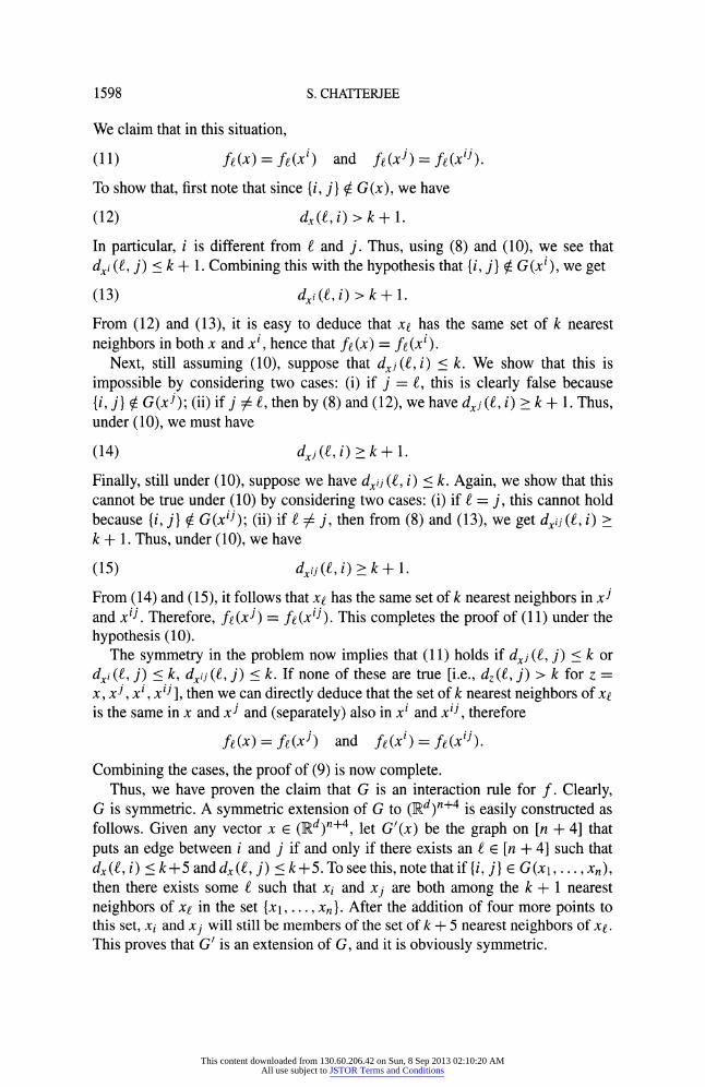
We claim that in this situation,
(11) fe(x) = f(x') and fe (xj) = ff (x'J).
To show that, first note that since {i, j} I G (x), we have
(12) d,(f, i) > k + 1. In particular, i is different from e and j. Thus, using (8) and (10), we see that dxi (f, j) < k + 1. Combining this with the hypothesis that {i, j} I G(x'), we get
(13) dxi (, i) > k + 1. From (12) and (13), it is easy to deduce that Xe has the same set of k nearest neighbors in both x and xi, hence that fe (x) = ft (xi).
Next, still assuming (10), suppose that dxj (f, i) < k. We show that this is impossible by considering two cases: (i) if j = -,
this is clearly false because {i, j} V G(xi); (ii) if j 0 f, then by (8) and (12), we have dxj (f, i) >
k + 1. Thus, under (10), we must have
(14) dxj(, i) >k + 1.
Finally, still under (10), suppose we have dxij (f, i) < k. Again, we show that this cannot be true under (10) by considering two cases: (i) if e = j, this cannot hold because {i, j} I G(x'J); (ii) if e : j, then from (8) and (13), we get dxij (f, i) > k + 1. Thus, under (10), we have
(15) dxi(, i) >k + 1. From (14) and (15), it follows that xe has the same set of k nearest neighbors in x1 and x'J. Therefore, fe (xj) = ft (x'l). This completes the proof of (11) under the hypothesis (10).
The symmetry in the problem now implies that (11) holds if dxj (f, j) < k or dxi (f, j) < k, dxij (f, j) < k. If none of these are true [i.e., dz (f, j) > k for z = x, xJ, xi, x i], then we can directly deduce that the set of k nearest neighbors of Xe is the same in x and xJ and (separately) also in x' and x'J, therefore
fe (X)= (xj) and fe (x') fe (x'J).
Combining the cases, the proof of (9) is now complete. Thus, we have proven the claim that G is an interaction rule for f. Clearly,
G is symmetric. A symmetric extension of G to (Rd)n+4 is easily constructed as follows. Given any vector x e (Rd)n+4, let G'(x) be the graph on [n + 4] that puts an edge between i and j if and only if there exists an e e [n + 4] such that dx (f, i) < k + 5 and dx (e, j) < k + 5. To see this, note that if {i, j } eG (x, ..., xn), then there exists some e such that xi and xj are both among the k + 1 nearest neighbors of Xe in the set {Xl,..., x, }. After the addition of four more points to this set, xi and xj will still be members of the set of k + 5 nearest neighbors of xe. This proves that G' is an extension of G, and it is obviously symmetric.
This content downloaded from 130.60.206.42 on Sun, 8 Sep 2013 02:10:20 AMAll use subject to JSTOR Terms and Conditions
A NEW METHOD OF NORMAL APPROXIMATION 1599
Now, for every x E Rd and 1 <j < n, let
Nj (x) :=- {: dx (f, j) < k}.
As we have noted before, if fe Nj (x) U Nj (xJ), then xe has the same set of k nearest neighbors in both x and xJ, therefore fe (x) = fj (xJ). Thus,
f (x) - f(xJ)
=- E n-1/2(f - f(x)).
eENj(x)UNj(xJ) It follows from standard geometrical arguments (see, e.g., [42], page 102) and the assumption that JIX1 - X2Ji is a continuous r.v. that INj(x) U Nj(xJ) I 2a(d)k, irrespective of n and x, where a (d) is the minimum number of 60' cones at the origin required to cover Rd. Thus, if we let
Mf := max Ife (X) I v max I f (xJ)I, f j,e
then the random variable M in the statement of Theorem 2.5 can be bounded by 4n-1/2a(d)kMf in this problem. Next, note that for any p > 8,
E(M)< [E(M)8p
<_ Y Elft(X)IP + -Eljfe(XJ)lp
_< (n 2+1 n)81
Lfj,f
Similarly, one can show that EI Aj f(X) 13 Ca(d)3k3n-3/2(nyp)3/p. Finally, note that by the same geometrical observation as mentioned before, the maximum degree of G'(X) is bounded by a(d)(k + 1)(k + 5). The proof is now completed by combining the bounds for all the terms and using Theorem 2.5. D
4. Proofs of the main results.
4.1. Proof of Theorem 2.2. Let us begin with the observation that, without loss of generality, we can replace f by a - f and then assume that a2 = 1. Henceforth, we will work under that assumption. The argument is divided into a sequence of lemmas. Lemmas 2.3 and 2.4 (already stated in Section 2) and Lemma 4.1 are original contributions of this paper, while Lemma 4.2 goes back to Stein [41].
PROOF OF LEMMA 2.3. Consider the sum 1
n A jf (XA)
AC [n] Al joA aC+[n] a,iA~i)'n --IAl) jQ~a
This content downloaded from 130.60.206.42 on Sun, 8 Sep 2013 02:10:20 AMAll use subject to JSTOR Terms and Conditions
1600 S. CHATTERJEE
Clearly, this is a linear combination of {f(XA), A C [n]}. It is a matter of simple verification that the positive and negative coefficients of f(XA) in this linear com- bination cancel out except when A = [n] or A = 0. In fact, the above expression is identically equal to f(X) - f(X').
Now, fix A and j 0 A, and let U = g(X)Ajf(XA). U is then a function of the random vectors X and X'. The joint distribution of (X, X') remains un- changed if we interchange Xj and X'. Under this operation, U changes to U':= -g(XJ)Aj f(XA). Thus,
]E(U) = E(U') = E(U + U')= -IE[Ajg(X)Ajf(XA)].
Combining these observations, we get
Cov(g(X), f (X)) = E[g(X)(f (X) - f(X'))]
= n CE[g(X)Ajf(XA)] -2lnl ( 1 )(n - IA
1 1
C > 1 (X) Aj f(XA)] A-[n]
( -
a j.A
This completes the proof of the lemma.
PROOF OF LEMMA 2.4. For each A C [n] and j a A, let
RA,j = Aj(ap o f)(X)Aj f(XA)
RA,j := p'(f (X))Aj f(X)Aj f (XA).
and
By Lemma 2.3 with g = ao o f, we have
1 1 (16) E(p(W)W) = - n
E(RA,j). 2 n]( )(n - JAI) Agn A jaA By the mean value theorem, we have
E|RA, j - RA, j| .El(Aj
f (X))2Aj
f (XA)]
IEIRAJ - RAl 2 l(f( A l (17)
< "EIAj f(X)13 (by Hilder's inequality). 2
Now, from the definition of T, we have
1 1 (18) y'(W)T
=- -
] n
- RA.
AC[n] (jA|)(n - jA
This content downloaded from 130.60.206.42 on Sun, 8 Sep 2013 02:10:20 AMAll use subject to JSTOR Terms and Conditions
A NEW METHOD OF NORMAL APPROXIMATION 1601
Combining (16), (17) and (18), we get
IE(Qp (W) W) - E(o'(W) T)
1An ~~E(RA, j - RA,j)
2
_
( 1(n)(n - AI) A A C[n] |A| joA < Inqo"1 > (n- lEA ijf(X)m
3 4 )(n - J(AI)) A_[n] A jP"
4 -
EIAj f(X)13
j=1
This completes the proof of the lemma. D]
LEMMA 4.1. Let W be as above. For any yO E C2(R) such that Il|o'll ~ 1 and Ila" lIa,
< 2, we have n
IE(o(W)W) - E(p'(W))I I [Var(E(TIW))]1/2 + 3Elj f (X)13. j=1
PROOF. Note that by putting g = f in Lemma 2.3, we get E(T) = E(W2) - 1. Since I|ap'lI ~ < 1, this gives
IE((p'(W)T) - E(p'(W))I <EIEE(TIW) - 1 < [Var(E(TIW))]1/2. The proof is completed by applying Lemma 2.4. D
LEMMA 4.2. Suppose h :R -* R is an absolutely continuous function with bounded derivative. Let Z - N (0, 1). There then exists a solution to the differential equation
pl'(x) - x p(x) = h(x) - Eh(Z)
that satisfies Il|'llj < V ||h'll| and II1p"ll| I 2 11h'l00. REMARK. It is not difficult to show that both constants are sharp. For a differ-
ent proof of the bound on lop' lloo, see Lemma 1 in [33]. The bound on 1l|0" loo is due to Stein ([41], page 27). Easier proofs with suboptimal constants can be found in Chen and Shao ([14], Chapter 1, Lemma 2.3).
PROOF OF LEMMA 4.2. It can be verified that the function
o(x) = ex2/2 xe-t2/2(h(t) - Eh(Z)) dt
= -ex2/2 f e-t2/2(h(t) - Eh(Z)) dt
This content downloaded from 130.60.206.42 on Sun, 8 Sep 2013 02:10:20 AMAll use subject to JSTOR Terms and Conditions
1602 S. CHATTERJEE
is a solution. Stein ([41], page 25, Lemma 3) proves that I1ap"11I < 2llh'llo0. The inequality I1a'11oo < II h'll, can also be derived using Stein's proof of the other inequality. We carry out the steps below. First, it is easy to verify that
h(x) - Eh(Z) = J h'(z)(z) dz - f h'(z)(1 - (z)) dz, -OO
where (D is the standard Gaussian c.d.f. Again, as proven in Stein ([41], page 27),
p(x) = - 2-7ex2/2(1 - ((x)) x
h'(z)d(z) dz
- vf7ex2/20(x) fx0h'(z)(1
- ((z))dz.
Combining, we see that
p'(x) = xa(x) + h(x) - Eh(Z)
=(1- V2-xex2/2(1 - 2
(x))) x
h'(z) 0(z) dz
- (1 + v xex2/2D(x))
fx0 h'(z)(1 - ( (z)) dz.
It follows that
Ilp'lloo < Ih'lloo sup 1- I - xe2/2(1 - x(x)
x
D(z) dz R ()( ())d)
N1 + ,/ x e x22/D(x) " (1 - (D(z))
dz. Using integration by parts, we get
x e-x2/2
00 (z) dz = xcI(x) +/2
fxo
e-x2/2 (1 - *(z))dz = -x(1 - (P(x)) - 2
and
Thus, we have
II'lloo _Ih'lloo
sup 1 - 2xex2/2(1 - D(x)) x(x) + e-2
+ 1 +V, xex2/2(x) (-x(1 - X(x)) + e2/2))
It is a calculus exercise to verify that the term inside the brackets attains its maxi- mum at x = 0, where its value is 2/1r. O
This content downloaded from 130.60.206.42 on Sun, 8 Sep 2013 02:10:20 AMAll use subject to JSTOR Terms and Conditions
A NEW METHOD OF NORMAL APPROXIMATION 1603
PROOF OF THEOREM 2.2. Take any h with IIh'll , < 1. Let yo be a solution to
ap'(x) - xp (x) = h(x) - Eh(Z). Then,
lEh(W) - Eh(Z) = E(P'(W)) - E(Wy(W)).
By Lemma 4.2, |II1o'|1 1 < 1 and 1Ip"Ill0 < 2. The proof is completed by applying Lemma 4.1. O
4.2. Proof of Theorem 2.5. By Theorem 2.2, our task reduces to obtaining a bound on Var(E(TIX)), where T is defined in (1). However, the situation in Theorem 2.5 is too complex to admit a direct computation of the variance. To circumvent this problem, we will use the following well-known martingale bound for the variance of an arbitrary function of independent random variables. This is known as the Efron-Stein inequality in the statistics literature.
LEMMA 4.3 ([17, 39]). Let Z = g(Y, ..., Ym) be a function of independent random objects Y1, ..., Ym. Let Yi' be an independent copy of Yi, i = 1,..., m. Then,
m
Var(Z) E[(g(YlI, .., Yi-, i',Y 1 ... Ym)- g(Yi,.., i=1
We will combine this inequality with another simple inequality that we were unable to locate in the literature.
LEMMA 4.4. If X and X' are independent random objects, then for any square integrable function U = g(X, X'), we have the inequality
Var(E(U IX)) < E(Var(U IX')).
PROOF. The proof is based on a simple application of Jensen's inequality. We just note that by the independence of X and X', we have IE(E(UIX') IX) = E(U) and therefore
Var(E(UIX)) = E(E(UIX) - E(U))2
= E(E(U - E(UIX')IX))2 < E(U - IE(UIX'))2 = IE(Var(UIX')).
This completes the proof of the lemma. O
Now, recall the definitions of A j, TA and T from Section 2, and the normal approximation bound in terms of Var(E(T IX)) in Theorem 2.2. We will prove the following upper bound on Var(E(TA IX)).
This content downloaded from 130.60.206.42 on Sun, 8 Sep 2013 02:10:20 AMAll use subject to JSTOR Terms and Conditions
1604 S. CHATTERJEE
LEMMA 4.5. With everything defined as before, we have
Var(E(TAIX)) < CE(M8)1I/2E(64)1/2 n(n - IAI), where C is a universal constant.
This is a good place to declare the convention that throughout the remainder of this section, C will denote numerical constants that do not depend on anything else and the value of C may change from line to line.
Before proving Lemma 4.5, we need to finish an important task.
PROOF OF THEOREM 2.2. Lemma 4.5, combined with Theorem 2.2, com- pletes the proof of Theorem 2.5 as follows. First, note that by the definition (1) of T and Minkowski's inequality, we have
1 [Var(E(TAIX))]1/2 [Var(E(TIX))]1/2 n - aC
n -2 A [n] iA|)(n--A
)
Substituting the bound from Lemma 4.5 into the above expression, we get
[Var(E(TIX))]'/2 < CE(M8)1/21E(4)1/2 n n -
AC[n] (A)(n - IL n
SCE(M8)1/2E(84)1/2 E n1/4k-3/4 k=l
< CE(M8)1/2E(84)1/2nl/2
This completes the proof of Theorem 2.5. O
Our main job now is to prove Lemma 4.5. Let us begin with a simple lemma about symmetric graphical rules.
LEMMA 4.6. Suppose G is a symmetric graphical rule on Xn and X = (X1, X2, ..., Xn) is a vector of independent and identically distributed X-valued random variables. Let dI be the degree of the vertex 1 in G(X). Take any k < n - 1 and let i, il, i2, ...--, ik be any collection of k + 1 distinct elements of [n]. Then,
E((d )k) (19) P({i, ie} E G(X) for each 1 <_ e
< k) = l (n - 1)k
where (r)k stands for the product r (r - 1)... (r - k + 1).
PROOF. Since G is a symmetric rule and the Xi's are i.i.d., the quantity
P({i, ie} E G(X) for all 1 < e < k)
This content downloaded from 130.60.206.42 on Sun, 8 Sep 2013 02:10:20 AMAll use subject to JSTOR Terms and Conditions
A NEW METHOD OF NORMAL APPROXIMATION 1605
does not depend on the specific choice of i, il, ..., ik. Hence,
IP({i, ie} E G(X) for each 1 < C < k) 1 I- IP({i, je} E G(X) for each 1 < C < k), (n - 1)k
where the sum is taken over all choices of distinct jl, ..., jk in [n]\{i}. Finally, note that
S]I{{i, je} E G(X) for each 1 < C < k} = (di)k, where di is the degree of the vertex i. Again, by symmetry, di and dl have the same distribution. This completes the argument. D
PROOF OF LEMMA 4.5. Fix a set A C [n]. For each j a A, let
Rj = Aj f(X)Aj f (XA)
= (f(X) - f (XJ))(f(XA) - f(XAUj)).
Now, let Y = (Y1,..., Y,) be another copy of X, independent of both X and X'. Fix 1 < i < n. Let
X (X1, ..., Xi-1, Yi, Xi+1, ..., Xn).
Similarly, for each B C [n], define XB by replacing Xi with Yi in XB. Explicitly, if i B, then
XB = (XB,..., X_1, Yi, , XB,..., XB),
whereas if i E B, then XB = XB. With this notation, let
Rji = (f (X) - f (X))(f(XA) - f(XAUj)),
hi := E((Rj - Rji)
and put
It follows from a combination of Lemmas 4.3 and 4.4 that n
(20) Var(E(TA IX)) < E(Var(TAIX')) Lhi. i=1
Let us now proceed to bound hi. First, take some j A U i and let
di = I{{i, j} E G(X)},
di = I{{i, j} E G(XJ)},
d3i -I{ {i, j} e G(X)}
This content downloaded from 130.60.206.42 on Sun, 8 Sep 2013 02:10:20 AMAll use subject to JSTOR Terms and Conditions
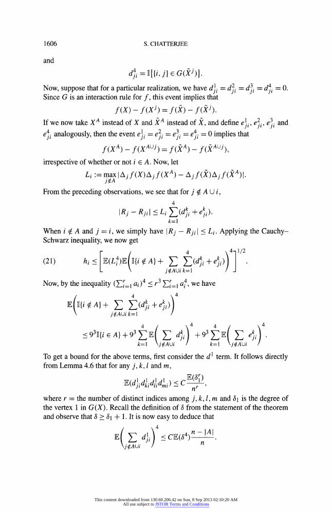
1606 S. CHATTERJEE
and
dj. = I{ {i, j} e G(Xj)}.
Now, suppose that for a particular realization, we have d.i
= d = d-i d - = 0.
Since G is an interaction rule for f, this event implies that
f (X) - f(Xj) = f(X) - f (XJ).
If we now take XA instead of X and XA instead of X, and define e j i ej i e and
e4i analogously, then the event ei = ei = e3i = ei==0 implies that
f (XA) _ f (XAUj) = f(XA) _ f(XAUj)
irrespective of whether or not i E A. Now, let
Li := max IAj f(X)Aj f(XA) - Aj f(X)Aj f(XA)1. joA
From the preceding observations, we see that for j 0 A U i, 4
JRj - Rji I Li 1(di
i +ei). k=l
When i 0 A and j = i, we simply have IRj - Rji[ Li. Applying the Cauchy- Schwarz inequality, we now get [ ( 4 4- 1/2 (21) hi < E(L4)E( {i 0 A) + E(dki + )e"i)
Lj AUi k=1 /
Now, by the inequality (r= ai)4 < r3 E a, we have --
i= Ia4 we have ( 4 4 E R~i 0Al}+ E E(dji +
eji)k jOAUi k=1
4 4 4 4
< 93I[{i E A} + 93' E di +93E Eei" k=l joAUi k=l joAUi
To get a bound for the above terms, first consider the d' term. It follows directly from Lemma 4.6 that for any j, k, I and m,
E(dd1d1d E(g) (dkididli dmi) < C , kt nr
where r = the number of distinct indices among j, k, 1, m and 61 is the degree of the vertex 1 in G(X). Recall the definition of S from the statement of the theorem and observe that S > 8 + 1. It is now easy to deduce that
4
joAUi n
This content downloaded from 130.60.206.42 on Sun, 8 Sep 2013 02:10:20 AMAll use subject to JSTOR Terms and Conditions
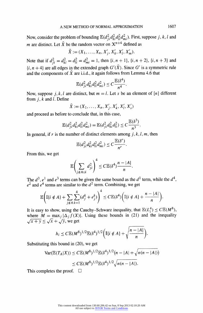
A NEW METHOD OF NORMAL APPROXIMATION 1607
Now, consider the problem of bounding E(dd i2i 2 d ). First, suppose j, k, 1 and m are distinct. Let X be the random vector on Xn+4 defined as
X :=
(Xl,..,
X,. , Xk, X, 9X/
Note that if d2i = dk2
= d2 = d2i - 1, then {i, n + 1}, {i, n + 21, {i, n + 31 and ji ki ii mi
{i, n + 41 are all edges in the extended graph G'(X). Since G' is a symmetric rule and the components of X are i.i.d., it again follows from Lemma 4.6 that
E (djidiidlidmi) < C E--- Sk n4 Now, suppose j, k, 1 are distinct, but m = 1. Let s be an element of [n] different from j, k and 1. Define
X := (X1,., Xn, Xj, Xk, X, X) and proceed as before to conclude that, in this case,
(ddkididmi) = E (d idli) C n3
. n3 In general, if r is the number of distinct elements among j, k, 1, m, then
E(d idk2id2i) < CE(Sr)
2 ) (joAUi j) -n
From this, we get
The d3, e1 and e3 terms can be given the same bound as the d1 term, while the d4 e2 and e4 terms are similar to the d2 term. Combining, we get ( k) 4 < C]E(64) + n -, JAI E
I{i a A} + --(d j + e ) < CE( {i A} n-|
joA k=l
It is easy to show, using the Cauchy-Schwarz inequality, that E(L4) < CE(M8), where M = maxj IAjf(X)1. Using these bounds in (21) and the inequality x + y < 1 + 4/Y, we get
hi < CE(M8)1/2E(34)1/2 (I{i A} + JA
Substituting this bound in (20), we get
Var(E(TAIX)) : CE(M8)1/2E(84)1/2(n - IA + n(n - AI))
< CE(M8)1/2E(84)1/2 n(n - I AI). This completes the proof.
This content downloaded from 130.60.206.42 on Sun, 8 Sep 2013 02:10:20 AMAll use subject to JSTOR Terms and Conditions
1608 S. CHATTERJEE
Acknowledgments. The author wishes to thank Persi Diaconis, Peter Bickel, Yuval Peres and the anonymous referee for many useful comments and sugges- tions.
REFERENCES
[1] ALDOUS, D. (1989). Probability Approximations via the Poisson Clumping Heuristic. Springer, New York. MR0969362
[2] AVRAM, F. and BERTSIMAS, D. (1993). On central limit theorems in geometrical probability. Ann. Appl. Probab. 3 1033-1046. MR1241033
[3] BALDI, P. and RINOTT, Y. (1989). On normal approximations of distributions in terms of dependency graphs. Ann. Probab. 17 1646-1650. MR1048950
[4] BALDI, P., RINOTT, Y. and STEIN, C. (1989). A normal approximation for the number of local maxima of a random function on a graph. In Probability, Statistics and Mathematics, Papers in Honor of Samuel Karlin (T. W. Anderson, K. B. Athreya and D. L. Iglehart, eds.) 59-81. Academic Press, Boston, MA. MR1031278
[5] BARBOUR, A. D. (1990). Stein's method for diffusion approximations. Probab. Theory Related Fields 84 297-322. MR1035659
[6] BICKEL, P. J. and BREIMAN, L. (1983). Sums of functions of nearest neighbor distances, moment bounds, limit theorems and a goodness of fit test. Ann. Probab. 11 185-214. MR0682809
[7] CACOULLOS, T., PAPATHANASIOU, V. and UTEV, S. A. (1994). Variational inequalities with examples and an application to the central limit theorem. Ann. Probab. 22 1607-1618. MR1303658
[8] CHATTERJEE, S. (2005). Concentration inequalities with exchangeable pairs. Ph.D. disserta- tion, Stanford Univ. Available at http://arxiv.org/math.PR/0507526.
[9] CHATTERJEE, S. (2006). Stein's method for concentration inequalities. Probab. Theory Re- lated Fields 138 305-321. MR2288072
[10] CHATTERJEE, S. (2008). Fluctuations of eigenvalues and second order Poincar6 inequalities. Probab. Theory Related Fields. To appear.
[11] CHATTERJEE, S. and FULMAN, J. Exponential approximation by exchangeable pairs and spec- tral graph theory. Submitted. Available at http://arxiv.org/abs/math/0605552.
[12] CHATTERJEE, S. and MECKES, E. Multivariate normal approximation using exchangeable pairs. Submitted. Available at http://arxiv.org/abs/math/0701464.
[13] CHEN, L. H. Y. and SHAO, Q.-M. (2004). Normal approximation under local dependence. Ann. Probab. 32 1985-2028. MR2073183
[14] CHEN, L. H. Y. and SHAO, Q.-M. (2005). Stein's method for normal approximation. In An Introduction to Stein's Method (A. D. Barbour and L. H. Y. Chen, eds.) 1-59. IMS (NUS) Lecture Notes 4. World Scientific, Hackensack, NJ. MR2235448
[15] DE JONG, P. (1987). A central limit theorem for generalized quadratic forms. Probab. Theory Related Fields 75 261-277. MR0885466
[16] DUPUIS, P., NUZMAN, C. and WHITING, P. (2004). Large deviation asymptotics for occu- pancy problems. Ann. Probab. 32 2765-2818. MR2078557
[17] EFRON, B. and STEIN, C. (1981). The jackknife estimate of variance. Ann. Statist. 9 586-596. MR0615434
[18] ENGLUND, G. (1981). A remainder term estimate for the normal approximation in classical occupancy. Ann. Probab. 9 684-692. MR0624696
[19] FELLER, W. (1968). An Introduction to Probability Theory and Its Applications. I, 3rd ed. Wiley, New York. MR0228020
This content downloaded from 130.60.206.42 on Sun, 8 Sep 2013 02:10:20 AMAll use subject to JSTOR Terms and Conditions
A NEW METHOD OF NORMAL APPROXIMATION 1609
[20] FRIEDRICH, K. 0. (1989). A Berry-Esseen bound for functions of independent random vari- ables. Ann. Statist. 17 170-183. MR0981443
[21] FULMAN, J. (2004). Stein's method and non-reversible Markov chains. In Stein's Method: Expository Lectures and Applications (P. Diaconis and S. Holmes, eds.) 69-77. IMS, Beachwood, OH. MR2118603
[22] GOLDSTEIN, L. and REINERT, G. (1997). Stein's method and the zero bias transformation with application to simple random sampling. Ann. Appl. Probab. 7 935-952. MR1484792
[23] GOLDSTEIN, L. and RINOTT, Y. (1996). On multivariate normal approximations by Stein's method and size bias couplings. J. Appl. Probab. 33 1-17. MR1371949
[24] GOTZE, F. and TIKHOMIROV, A. N. (1999). Asymptotic distribution of quadratic forms. Ann. Probab. 27 1072-1098. MR1699003
[25] GOTZE, F. and TIKHOMIROV, A. N. (2002). Asymptotic distribution of quadratic forms and applications. J. Theoret. Probab. 15 423-475. MR1898815
[26] HAAGERUP, U. (1982). The best constants in the Khintchine inequality. Studia Math. 70 231- 283. MR0654838
[27] HALL, P. (1984). Central limit theorem for integrated square error of multivariate nonparamet- ric density estimators. J. Multivariate Anal. 14 1-16. MR0734096
[28] HALL, P. (1988). Introduction to the Theory of Coverage Processes. Wiley, New York. MR0973404
[29] KESTEN, H. and LEE, S. (1996). The central limit theorem for weighted minimal spanning trees on random points. Ann. Appl. Probab. 6 495-527. MR1398055
[30] LEVINA, E. and BICKEL, P. J. (2005). Maximum Likelihood Estimation ofIntrinsic Dimension. In Advances in NIPS 17 (L. K. Saul, Y. Weiss and L. Bottou, eds.) 777-784. MIT Press, Cambridge, MA.
[31] PENROSE, M. D. (2003). Random Geometric Graphs. Oxford Univ. Press. MR1986198 [32] PENROSE, M. D. and YUKICH, J. E. (2001). Central limit theorems for some graphs in com-
putational geometry. Ann. Appl. Probab. 11 1005-1041. MR1878288 [33] RAIC, M. (2004). A multivariate CLT for decomposable random vectors with finite second
moments. J. Theoret. Probab. 17 573-603. MR2091552 [34] RINOTT, Y. and ROTAR, V. (1996). A multivariate CLT for local dependence with n-1/2 logn
rate and applications to multivariate graph related statistics. J. Multivariate Anal. 56 333- 350. MR1379533
[35] RINOTT, Y. and ROTAR, V. (1997). On coupling constructions and rates in the CLT for depen- dent summands with applications to the antivoter model and weighted U-statistics. Ann. Appl. Probab. 7 1080-1105. MR1484798
[36] RINOTT, Y. and ROTAR, V. (2003). On edgeworth expansions for dependency-neighborhoods chain structures and Stein's method. Probab. Theory Related Fields 126 528-570. MR2001197
[37] ROTAR, V. I. (1973). Some limit theorems for polynomials of second degree. Theory Probab. Appl. 18 499-507. MR0326803
[38] RUSCHENDORF, L. (1985). Projections and iterative procedures. In Multivariate Analysis VI (P. R. Krishnaiah, ed.) 485-493. North-Holland, Amsterdam. MR0822314
[39] STEELE, J. M. (1986). An Efron-Stein inequality for nonsymmetric statistics. Ann. Statist. 14 753-758. MR0840528
[40] STEIN, C. (1972). A bound for the error in the normal approximation to the distribution of a sum of dependent random variables. Proc. of the Sixth Berkeley Symp. Math. Statist. Probab. II. Probability Theory 583-602. Univ. California Press, Berkeley. MR0402873
[41] STEIN, C. (1986). Approximate Computation ofExpectations. IMS Lecture Notes-Monograph Series 7. IMS, Hayward, CA. MR0882007
[42] YUKICH, J. E. (1998). Probability Theory of Classical Euclidean Optimization Problems. Lec- ture Notes in Math. 1675. Springer, Berlin. MR1632875
This content downloaded from 130.60.206.42 on Sun, 8 Sep 2013 02:10:20 AMAll use subject to JSTOR Terms and Conditions

1610 S. CHATTERJEE
[43] VAN ZWET, W. R. (1984). A Berry-Esseen bound for symmetric statistics. Z. Wahrsch. Verw. Gebiete 66 425-440. MR0751580
DEPARTMENT OF STATISTICS UNIVERSITY OF CALIFORNIA AT BERKELEY 367 EVANS HALL #3860 BERKELEY, CALIFORNIA 94720-3860 USA E-MAIL: [email protected] URL: http://www.stat.berkeley.edu/-sourav/
This content downloaded from 130.60.206.42 on Sun, 8 Sep 2013 02:10:20 AMAll use subject to JSTOR Terms and Conditions