A New Method for Material Point Method Particle Updates that ReducesNoise and Enhances Stability

Chad C. Hammerquista, John A. Nairna,∗

aWood Science and Engineering, Oregon State University, Corvallis, OR 97330, USA

Abstract

Current material point method (MPM) particle updates use a PIC approach, a FLIP approach, or a linearcombination of PIC and FLIP. A PIC update filters velocity in each time step, which causes unwantednumerical diffusion, while FLIP eliminates that diffusion, but may retain too much noise. This paperdevelops a new particle update termed XPIC(m) (for eXtended PIC of order m) because it generalizes PICupdates. XPIC(1) is identical to current PIC methods, but higher orders of XPIC(m) address the overfiltering and numerical diffusion of PIC, while still filtering out noise caused by the nontrivial null space ofthe extrapolation matrix used in MPM. As m → ∞, XPIC(m) converges to a modified FLIP update withorthogonal removal of null space noise. The frequency response and filtering properties of XPIC(m) areinvestigated and several numerical examples demonstrate its advantages over other update methods.

Keywords: Material Point Method, Null Space, Computational Mechanics

1. Introduction

The Material Point Method (MPM) is a solid mechanics numerical tool that is well suited for solvingproblems involving complex geometries, large deformations, history-dependent materials, and contact. Themethod is a hybrid Eulerian-Lagrangian formulation where a modeled object is discretized into a set ofmaterial points or particles. Information needed to solve the equations of motions is extrapolated back andforth between material points and a background grid. MPM has been able to simulate a diverse array ofcomplex problems. A partial list includes modeling complex biological structures [1] (including resolvingcellular structure of wood [2–4]), granular materials [5], land slides and avalanches [6], explosive welding [7],cutting simulations [8, 9], sea ice dynamics [10], snow dynamics [11] and fracture simulations [12, 13].

Each dynamic MPM time step interpolates particle information to the grid, solves equations of motionon the grid, and then updates particle properties including stress, strain, plastic or damage history variables,velocity, and position. When updating velocity and position, two methods (or a mixture of the two) arecurrently available — Particle In Cell (or PIC) and FLuid Implicit Particle (or FLIP). PIC was developedby Harlow [14]. Although stable, it filters velocities that can lead to overdamping of kinetic energy indynamic problems. FLIP was developed by Brackbill et al. [15, 16] to reduce dissipation by eliminatingvelocity filtering. It can, however, introduce noise that eventually reduces stability. PIC and FLIP particlemethods, which were derived for fluids, were extended to solid mechanics by MPM [17]. The original MPMused FLIP methods and they remain the standard MPM particle update method.

Attempts to reduce FLIP noise include using a convex combination of FLIP and PIC [9, 11] and using asmoothing operator for spatial gradients [18]. While these approaches do reduce noise, they still suffer fromunwelcome damping. Here, we propose a new method referred to as eXtended PIC or XPIC(m) of orderm = 1 to ∞. XPIC(1) is identical to current PIC methods, which over filters velocities and may dissipatekinetic energy. As m → ∞, XPIC(m) asymptotically approaches a modified FLIP update that removesall noise associated with the null space of the extrapolation matrix. This limit provides an optimal updatemethod for MPM with ideal frequency properties, i.e, removal of null space noise without causing numericaldiffusion or reducing accuracy

∗Corresponding author: john.nairn@oregonstate.edu, Tel: +1-541-737-4265, Fax: +1-541-737-3385

Preprint submitted to Elsevier February 17, 2017

Section 2 rederives FLIP and PIC velocity updates using inverse problem methodology. We then showthat the new XPIC(m) method can be derived as a natural extension of that framework simply by revisingthe constraint in the inverse problem. The frequency response of XPIC(m) updates are examined along withconvergence of XPIC(m) to orthogonal null space removal. Finally, Section 3 gives example problems thatdemonstrate some XPIC(m) properties and show advantages of XPIC(m) over prior methods.

2. Numerical Methods

2.1. MPM Extrapolations

MPM is based on a dual representation of a modeled object — a Lagrangian view (particles) and anEulerian view (grid). The particles carry conserving quantities such as mass, momentum and (possibly)history-dependent material properties. Momenta and gradient information are computed on the grid andused to solve the momentum equation. In each time step, updated grid information (or Eulerian frame) Gis linearly mapped to the particle space (or Lagrangian frame) P :

S : G → P (1)

where S is a matrix of interpolation coefficients. To create this array, the grid space is expanded in anapproximate basis of “grid shape functions,” denoted here as Ni(x) for node i. The particle space is expandedin an approximate basis of “particle shape functions,” that are based on a particle’s position and domainand denoted here as χp(x) for particle p (it is typically 1 within the particle domain and zero elsewhere).The final MPM shape functions are created by convolution of these two bases [19].

Spi(x) =

∫χp(x)Ni(x)dx∫χp(x)dx

(2)

These MPM shape functions define the elements Spi of the S matrix corresponding to particle p and node i.These shape functions have partition of unity on the grid:∑

i

Spi = 1 ∀p. (3)

The simplest mapping is a nearest grid point interpolation (NGP), where particles map all their infor-mation to their nearest grid node. In one dimension of a regular grid with cell size ∆x, NGP interpolationcorresponds to grid shape functions that are “box-car” functions ( or Ni(x) = rect((x − xi)/∆x) fornode at xi), and particle shape functions that are Dirac delta functions ( or χp(x) = δ(x − xp) for par-ticle at xp). The FLIP and PIC precursors to MPM were developed around these shape functions [14–16].The original development of MPM replaced “box-car” functions with overlapping tent functions ( orNi(x) = tri((x − xi)/∆x)) and retained Dirac delta functions ( ) on the particles [17]. The resultingMPM shape functions are in C0, but their discontinuous derivatives cause problems when particles cross cellboundaries. The generalized interpolation material point (GIMP) shape functions [19] were developed, inpart, to improve cell-crossing issues. GIMP’s mapping convolves overlapping tent functions ( ) on thegrid with “box-car” functions ( or χp = rect((x − xp)/lp) where lp is current length of the particledomain) on the particles. The resulting MPM shape functions are very similar to quadratic b-splines and arein C1. Other possible shape functions include CPDI [20], higher order b-splines [21], and many undevelopedones that could be derived by GIMP methods [19].

The S matrix maps from the grid to the particles, but MPM also needs to map from the particles tothe grid. When velocity is mapped from the particles to the grid, it is in the form of momentum. Thisextrapolation results in a mass-weighted mapping of particle velocities (V ) to grid velocities (v) of:

S+ : P → G =⇒ v = S+V (4)

where all MPM implementations use [17]:

S+ = DSTM, Dn×n = diag

(1

STM

), and MN×N = diag (M)

(i.e., S+

ip =MpSpi∑MpSpi

)(5)

2

where M is a vector of particle masses (Mp) and n and N are the number of nodes and particles, respectively.Throughout this paper we use lower case letters for grid quantities and upper case letters for particlequantities. Much MPM literature is based on the corresponding extrapolation of particle momentum (P )to the grid using p = STP and elements STip are often denoted as Sip; we changed this prior notation to the

more consistent STip = Spi.

In each MPM time step, S+ maps particle velocities to the grid and S maps them back. The mappingand its reverse come naturally from the variational framework of MPM [19] and was originally derived bya weighted, least-squares analysis of extrapolation followed by using a lumped mass matrix to derive theabove elements of S+ [17]. A better approach would be to find S+ by inverting S, but that approach hastwo problems. First, the number of particles is usually greater than the number of grid nodes in play,which means the S matrix is neither square nor invertible. Second, dealing with non-square S by finding ageneralized Moore-Penrose inverse [22] on each time step would be prohibitively expensive. In contrast, thecurrent reverse mapping in Eq. (5) is very efficient; in fact, it is almost free.

If the standard MPM shape functions are replaced by the simpler NGP shape function, and all particleshave the same mass, we have observed that S+ in Eq. (5) is the exact Moore-Penrose inverse of S (seetheorem 1 in the Appendix). Furthermore, an NGP analysis for velocity updates can be posed as a suiteof inverse problems with exact solutions. By changing the constraint in the problem, various analyses leadto FLIP, PIC, or the new XPIC(m) update methods. For non-NGP interpolations, or when particles havedifferent masses, the inverse solutions are no longer exact (or S+ is no longer the exact generalized inverseof S), but the derived update methods can be treated as approximate solutions.

2.2. FLIP and PIC Derivations by Inverse Methodology

Although literature derivation of FLIP [15, 16] and PIC [14] updates were done differently, we show howto derive them using inverse methodology. Starting with a vector of updated velocities on the grid:

v(k+) = v(k) + a(k)∆t (6)

where v(k) and a(k) are velocity and acceleration vectors on the grid in time step k, the MPM update needsto find particle velocities by inverting the particle-to-grid extrapolation:

S+V (k+1) = v(k+) (7)

In general, there are more particles than active grid points, so Eq. (7) has an infinite number of solutions.To get a unique solution some constraint must be added. One choice is to constrain the new particle velocityto be close to the previous velocity, which gives this inverse problem:

V (k+1) = argminV

‖V − V (k)‖2 such that: S+V = v(k+) (8)

It follows from Theorem 2 in the Appendix that Eq. (8) has the solution:

V (k+1) = Sv(k+) + (I− SS+)V (k) (9)

Rewriting Eq. (9) gives:

V (k+1) = S(a(k)∆t+ S+V (k)) + (I− SS+)V (k) = V (k) + Sa(k)∆t (10)

which is the usual FLIP update [9, 11] (i.e., increment particle velocity by acceleration extrapolated fromthe grid).

Another constraint choice, which will give a new style update, is to constrain magnitude of the updatedvelocity vector to be as small as possible:

V (k+1) = argminV

‖V ‖2 such that: S+V = v(k+) (11)

which from Theorem 2 in the Appendix has the solution:

V (k+1) = Sv(k+) (12)

3

This update is the usual PIC update [9, 11] (i.e., replace particle velocity with velocity extrapolated fromthe grid). This formulation helps explain PIC dissipation — it is trying to drive the velocities towards zeroin order to minimize its constraint. It achieves this minimization by diffusing the velocities and therebydissipating kinetic energy.

Each MPM time step needs to update both particle velocity and position. Those updates can be writtenin a generalized form that accommodates FLIP and PIC updates as:

V (k+1) = V (k) +

∫ ∆t

0

A(k) dt = V (k) + A(k)∆t (13)

X(k+1) = X(k) +

∫ ∆t

0

(Sv(k) + A(k)t

)dt = X(k) + Sv(k+)∆t+

(1

2A(k) − Sa(k)

)(∆t)2 (14)

where A(k) is an effective acceleration for the chosen update method. The integrals were found by mid-point rule with A(k) and v(k) constant over the time step. FLIP or PIC style updates use these effectiveaccelerations:

A(k) = Sa(k) (FLIP) (15)

A(k) = Sa(k) − (I− SS+)V (k)

∆t(PIC) (16)

The PIC effective acceleration is the acceleration needed to replace particle velocity with velocity extrapolatedfrom the grid. Obviously, a linear combination of FLIP and PIC [9, 11] uses:

A(k) = Sa(k) − fPIC(I− SS+)V (k)

∆t(17)

where fPIC is fraction PIC in the update. Many MPM codes simplify to a first order position update— X(k+1) = X(k) + Sv(k+)∆t. Although this approach works to first order for pure FLIP updates, it isunacceptable for a generalized update including both FLIP and PIC. When using some PIC, the apparentlysecond order (∆t)2 term in Eq. (14) expands to include a first order term [9], which implies that a generalizedposition update has to be second order.

2.3. XPIC(m) Derivation

Alternatives to FLIP and PIC updates can be derived by changing the constraint imposed on the inverseproblem. The goals for a new update method are to reduce both velocity diffusion caused by PIC andnoise caused by FLIP. A potential constraint to achieve these goals is to minimize the difference betweennew velocity V (k+1) and a smoothed previous velocity V sm. The justification is that minimizing a velocitydifference reduces velocity diffusion while differencing with a smoothed velocity may reduce noise. Theinverse problem becomes:

V (k+1) = argminV

‖V − V sm‖2 such that: S+V = v(k+) (18)

which for NGP shape functions has the exact solution:

V (k+1) = Sv(k+) + (I− SS+)V sm (19)

An efficient (and effective) method to derive a smoothed velocity is to extrapolate initial grid velocity

back to the particles or V sm = Sv(k) = SS+V (k). Using this smoothing, the update in Eq. (19) becomes:

V (k+1) = Sv(k) + (I− SS+)SS+V (k) (20)

This update leads to a new effective acceleration for particle updates:

A(k) = Sa(k) − (I− SS+)2V (k)

∆tXPIC(2) (21)

4

The only difference between XPIC(2) and PIC is that the (I− SS+) term is now squared (hence the “2” inXPIC(2)). We are led to propose a generalized XPIC(m) method with an effective acceleration of:

A(k) = Sa(k) − (I− SS+)mV (k)

∆tXPIC(m) (22)

Comparing to Eq. (19), XPIC(m) corresponds to using the smoothed velocity:

V sm =((I− (I− SS+)m−1

)V (k) (23)

The physical significance of this result is addressed below.The above NGP derivations for FLIP, PIC, and XPIC(m) are exact inverse problem solutions (for special

case of all particles having the same mass). When NGP solutions are replaced by MPM shape functions (orfor particles with different masses), the updates are no longer exact solutions to the inverse problems, butcan be interpreted as approximate solutions under the specified constraints. Insights from those constraintsreveal that PIC filters out too much velocity to meet its constraint to minimize velocity vector magnitudewhile FLIP eliminates that filtering, but may retain too much noise. Our new XPIC(m) method introducesminimization to a constraint based on difference with a smoothed velocity that may both minimize dissipationand reduce noise.

2.4. XPIC(m) Properties

To quantify XPIC(m) performance, we considered its spatial filtering properties. Updated particle veloc-ities can be written as filtered particle velocities from the previous step plus extrapolated grid acceleration:

V (k+1) = PV (k) + Sa(k)∆t (24)

where P is a projection matrix that defines the particle velocity filtering. The projection P is determined bythe update method:

P = I FLIP (25)

P = SS+ PIC (= XPIC(1)) (26)

P = I− (I− SS+)m XPIC(m) (27)

It is evident that PIC and XPIC(m) updates filter velocities while FLIP does no filtering. As done inRefs. [14–16], consider a simple 1D example with N particles of equal mass, evenly spaced by ∆x, andclassic MPM linear shape functions. The velocity of particle p = 0 to N − 1 can be represented in spatialfrequency space by:

Vp =1

N

(v0 +

N−1∑k=1

vke2πikp/N

)where vk =

N−1∑p=0

Vpe−2πikp/N (28)

are coefficients from discrete Fourier transform of the particle velocities. When PIC or XPIC(m) is used inMPM, the velocities are convolved in each step with the above filtering matrix P. The filtered velocity ofparticle p becomes:

(PV )p =1

N

(v0 +

N−1∑k=1

Pkvke2πikp/N

)(29)

Here, the Pk ∈ [0, 1] coefficients represent damping coefficient at each spatial frequency. Due to shapefunction properties, the constant velocities are undamped. The Fourier transform of the linear shape functionmapping of this problem to the grid is given as:

Pk = sinc2(k∆x) (30)

where sinc(x) = sin(xπ)/(xπ). This transform also holds for mapping back to the particles. Therefore theFourier transform of the P matrix for PIC with linear shape functions is given as:

Pk = sinc4(k∆x) (31)

5

Wave Number

Atte

nuat

ion

0.0 0.1 0.2 0.3 0.4 0.5 0.6 0.0 0.1

0.2

0.3

0.4

0.5

0.6

0.7

0.8

0.9

1.0

1.1

m=1

2

5

10 1520

FLIP25

NullSpace

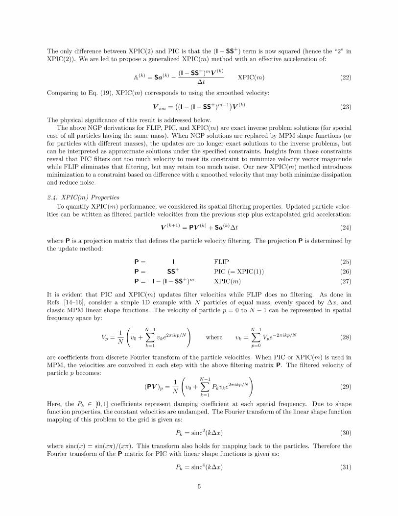
Figure 1: Frequency Response of FLIP, PIC (or XPIC(1)) and several orders of XPIC(m) in one dimension with evenly spacedparticles of equal mass, and the classic MPM shape functions. The shaded area is the null space that is removed by PIC andXPIC(m),

Following this logic, the Fourier transform for XPIC(m) filtering matrix P is given as:

Pk = 1−(1− sinc4(k∆x)

)m(32)

The frequency responses for FLIP, PIC, and XPIC(m) are plotted in Fig. 1. Because FLIP does nofiltering, its response is a horizontal line for all frequencies. Given the discretization of the filtering, bothPIC and XPIC(m) completely remove all null space components, which is plotted as frequency responsedropping to zero for wave number greater than 0.5 (i.e, wavelength equal to the size of two grid cells), whichcorresponds to the Nyquist sampling frequency on the grid. The responses for PIC and XPIC(m) differ forwave number less than 0.5. For PIC, all the frequencies, except the constant velocity, are damped. Thisfrequency response explains the large diffusion caused by PIC. In contrast, the XPIC(m) frequency responsehas a larger region with little or no damping. Even XPIC(2), for example, has very little attenuation forany frequencies with a wave number less than 0.1 (i.e, wavelength greater than 10 grid cells). As m grows,the frequency response for XPIC(m) converges to a brick-wall filter at the null space of S+.

If m → ∞ (and all particles have the same mass), XPIC(m) converges to exact orthogonal null spaceremoval, regardless of shape function type, problem dimension, or spatial distribution of the particles. Inother words, Theorem 3 in the Appendix shows that:

limm→∞

(I− SS+)m = Ω (33)

where Ω is an orthogonal projection onto the null space of S+. The null space N (S+) of matrix S+ is thelinear subspace of all vectors that S+ maps to zero:

S+z = 0 ∀z ∈ N (S+). (34)

Conceptually, N (S+) represents all velocity modes on the particles that are not mapped to the grid. Sub-stituting into Eq. (27), as m→∞, the XPIC(m) filtering matrix becomes

P = I−Ω (35)

which is an orthogonal projection onto the orthogonal complement of the null space of S+. Any velocitymodes (and only those modes) invisible to the grid are removed by this filtering. Consequently the grid

6

m

Rel

ativ

e E

rror

0 1 2 3 4 5 6 7 8 9 10 11 12 13 14 15 0.0

0.1

0.2

0.3

0.4

0.5

PIC

XPIC(2)

XPIC(3)

XPIC(4)

k (I SS+)mkFkkF

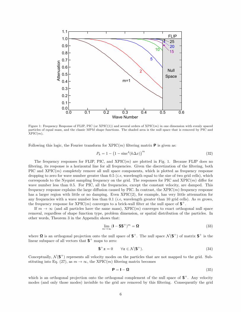
Figure 2: Convergence of (I − SS+)m to Ω for 1D example with 50 particles. The relative error is the equation shown on theplot,

space G and the particle space P are on the same page, working with the same information after the leastpossible amount of damping. The physical significance of Eq. (23) now is that XPIC(m) minimizes differencebetween updated velocity and previous velocity with null space modes removed.

For finite m in calculations, XPIC(m) for increasing m represents successive approximations to orthogonalnull space removal. To test the convergence, we built a simple 1D example with 50 equally-spaced particlesusing linear shape functions. For this simple example, we could use singular value decomposition (SVD)to exactly calculate the null space projection operator, Ω. Figure 2 plots normalized magnitude of thedifference between (I − SS+)m and the exact Ω as a function of the XPIC(m) order. The results showgeometric convergence to the null space projection (i.e., log(||Ω− (I− SS+)m||F ) converges linearly in m).

Convergence to Ω is significant because previously an orthogonal null space removal would require amatrix decomposition in each time step, which has computational cost of O(N3) [18, 23]. Due to sparsityof S, the XPIC(m) method scales linearly in the number of particles (see section 2.5). If some particleshave different mass, Eq. (33) is no longer exact, but instead converges to an oblique projection onto thenull space of S+. Our numerical experiments, however, suggest nearly identical effects. Furthermore, acommon approach to MPM when modeling particles of different materials having different densities (andhence different masses) is to use multiple velocity fields — one velocity field for each material type [24]. Inthis so-called multimaterial mode MPM, each velocity field updates separately and normally uses constant-mass particles. The XPIC(m) method should therefore approach the appropriate null space removal. Thevelocity fields interact by contact [24] or interface laws [25] that act as boundary conditions to those fields.

2.5. Implementation Details

The details for efficiently (as possible) implementing XPIC(m) are given here. The particle effectiveacceleration for XPIC(m) is:

A(k)∆t = Sa(k)∆t− (I− SS+)mV (k) = Sa(k)∆t− V (k) +mSv(k) −mSv∗ (36)

where

v∗ =1

m

m∑r=2

(m

r

)(−1)r(S+S)r−1v(k) =

m∑r=2

(−1)rv∗r (37)

7

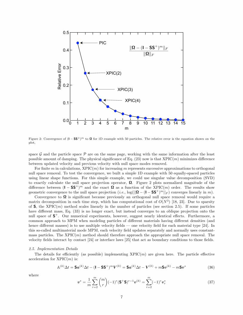
Table 1: To calculate v∗ allocate space for three velocities on each node (v∗, v−, and v+) and use the algorithm presentedin this table. For the inner i and j loops, ϑp is the set of nodes k : Spk 6= 0 or nodes for particle p with non-zero shapefunction — this set will have a small number of members and its size will be independent of problem size.

let v∗ ← 0 and v− ← v(k+) − a(k)∆tfor each r in 2 to m do

let v+ ← 0for each p in N do

for each i in ϑp dofor each j in ϑp do

let (v+)i ← (v+)i + m−r+1r

MpSpiSpj

m(k)i

(v−)j

let v∗ ← v∗ + (−1)rv+ and v− ← v+

One could include grid or particle damping, such as described in Ref. [9], but those terms are omitted hereto focus on XPIC(m) terms. The new v∗ term, which is unique to XPIC(m) with m > 1, can be evaluatedby recursion:

v∗r =1

m

(m

r

)(S+S)r−1v(k) =

1

m

(m

r

)S+S(S+S)r−2v(k) =

m− r + 1

rS+Sv∗r−1 (38)

starting with v∗1 = v(k).In typical MPM codes, the particle update is done after v(k+) has replaced v(k). Using only updated

grid velocities, the recursion relation starts with v∗1 = v(k+)−a(k)∆t and the effective acceleration becomes:

A(k)∆t = (1−m)Sa(k)∆t− V (k) +mSv(k+) −mSv∗ (39)

Explicit particle updates for position and velocity are:

V (k+1) = V (k) +(

Sa(k) − a(k)ex

)∆t (40)

X(k+1) = X(k) + Sv(k+)∆t−(

Sa(k) + a(k)ex

) (∆t)2

2(41)

where a(k)ex appears as a “damping” term, but here is implementing XPIC(m):

a(k)ex ∆t = −mS

(v(k+) − a(k)∆t

)+ V (k) +mSv∗ (42)

Note again, that while many MPM codes stop the position update with the first term involving updated gridvelocities, the implementation of XPIC(m) requires the apparent second order term because part of thatterm evaluates to first order.

For most MPM codes, the addition of an XPIC(m) option reduces to a new calculation of v∗ just beforethe particle update; pseudocode for that calculation is given in Table 1. The increment in v+ correspondsto the evaluation of v∗r by Eq. (38) on node i:

(v∗r)i =m− r + 1

r

∑p

MpSpi

m(k)i

(Sv∗r−1)p =m− r + 1

r

∑p

∑j

MpSpiSpj

m(k)i

(v∗r−1)j (43)

Due to sparsity of S, the number of nodes needed for the i and j loops will be small and independent ofthe problem’s size. The calculation therefore scales linearly with the XPIC(m) order times the number ofparticles (N) (linearly with mN) and is easily parallelized.

3. Results and Discussion

This section presents examples that show improvements of XPIC(m) methods over existing methods anddemonstrate some XPIC(m) properties.

8

Horizontal Dimension (mm)

Velo

city

(m/s

)

0 20 40 60 80 100 120 140 160 -0.08

-0.04

0.00

0.04

0.08

0.12

0.16

0.20

0.24 FLIP

PIC

XPIC(15)

XPIC(2)A

FLIP

Time (ms)

Velo

city

(m/s

)

0.00 0.02 0.04 0.06 0.08 0.10 0.12 0.14 -0.05

-0.00

0.05

0.10

0.15

0.20

0.25 FLIP

XPIC(2)

PIC

B

FLIPXPIC(2)

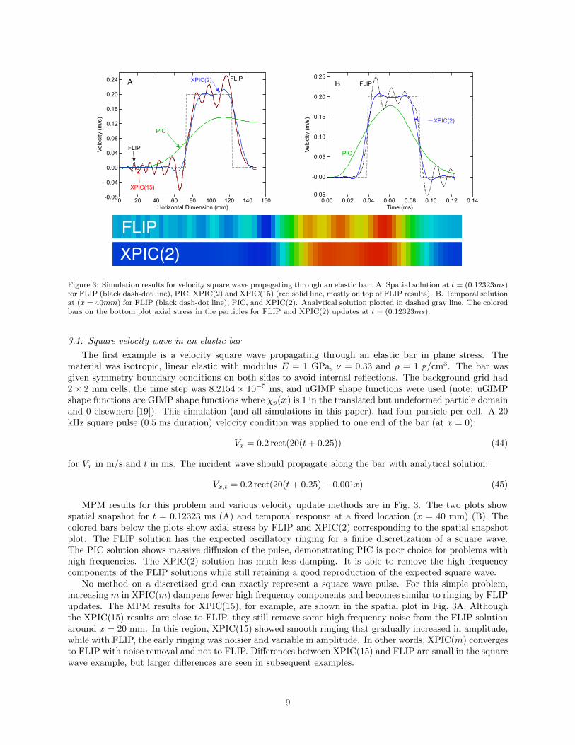
Figure 3: Simulation results for velocity square wave propagating through an elastic bar. A. Spatial solution at t = (0.12323ms)for FLIP (black dash-dot line), PIC, XPIC(2) and XPIC(15) (red solid line, mostly on top of FLIP results). B. Temporal solutionat (x = 40mm) for FLIP (black dash-dot line), PIC, and XPIC(2). Analytical solution plotted in dashed gray line. The coloredbars on the bottom plot axial stress in the particles for FLIP and XPIC(2) updates at t = (0.12323ms).

3.1. Square velocity wave in an elastic bar

The first example is a velocity square wave propagating through an elastic bar in plane stress. Thematerial was isotropic, linear elastic with modulus E = 1 GPa, ν = 0.33 and ρ = 1 g/cm3. The bar wasgiven symmetry boundary conditions on both sides to avoid internal reflections. The background grid had2× 2 mm cells, the time step was 8.2154× 10−5 ms, and uGIMP shape functions were used (note: uGIMPshape functions are GIMP shape functions where χp(x) is 1 in the translated but undeformed particle domainand 0 elsewhere [19]). This simulation (and all simulations in this paper), had four particle per cell. A 20kHz square pulse (0.5 ms duration) velocity condition was applied to one end of the bar (at x = 0):

Vx = 0.2 rect(20(t+ 0.25)) (44)

for Vx in m/s and t in ms. The incident wave should propagate along the bar with analytical solution:

Vx,t = 0.2 rect(20(t+ 0.25)− 0.001x) (45)

MPM results for this problem and various velocity update methods are in Fig. 3. The two plots showspatial snapshot for t = 0.12323 ms (A) and temporal response at a fixed location (x = 40 mm) (B). Thecolored bars below the plots show axial stress by FLIP and XPIC(2) corresponding to the spatial snapshotplot. The FLIP solution has the expected oscillatory ringing for a finite discretization of a square wave.The PIC solution shows massive diffusion of the pulse, demonstrating PIC is poor choice for problems withhigh frequencies. The XPIC(2) solution has much less damping. It is able to remove the high frequencycomponents of the FLIP solutions while still retaining a good reproduction of the expected square wave.

No method on a discretized grid can exactly represent a square wave pulse. For this simple problem,increasing m in XPIC(m) dampens fewer high frequency components and becomes similar to ringing by FLIPupdates. The MPM results for XPIC(15), for example, are shown in the spatial plot in Fig. 3A. Althoughthe XPIC(15) results are close to FLIP, they still remove some high frequency noise from the FLIP solutionaround x = 20 mm. In this region, XPIC(15) showed smooth ringing that gradually increased in amplitude,while with FLIP, the early ringing was noisier and variable in amplitude. In other words, XPIC(m) convergesto FLIP with noise removal and not to FLIP. Differences between XPIC(15) and FLIP are small in the squarewave example, but larger differences are seen in subsequent examples.

9

FL

IPX

PIC

(15)

t = 0.5 ms t = 2 ms t = 10 ms t = 22.5 ms

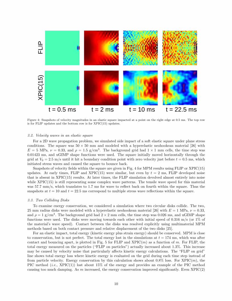
Figure 4: Snapshots of velocity magnitudes in an elastic square impacted at a point on the right edge at 0.5 ms. The top rowis for FLIP updates and the bottom row is for XPIC(15) updates.

3.2. Velocity waves in an elastic square

For a 2D wave propagation problem, we simulated side impact of a soft elastic square under plane stressconditions. The square was 50 × 50 mm and modeled with a hyperelastic neohookean material [26] withE = 5 MPa, ν = 0.33, and ρ = 1.5 g/cm3. The background grid had 1 × 1 mm cells, the time step was0.01423 ms, and uGIMP shape functions were used. The square initially moved horizontally through thegrid at V0 = 2.5 m/s until it hit a boundary condition point with zero velocity just before t = 0.5 ms, whichinitiated stress waves and caused the square to bounce back.

Snapshots of velocity fields within the square are given in Fig. 4 for MPM results using FLIP or XPIC(15)updates. At early times, FLIP and XPIC(15) were similar, but even by t = 2 ms, FLIP developed noisethat is absent in XPIC(15) results. At later times, the FLIP simulation devolved almost entirely into noisewhile XPIC(15) is still representing some complex wave patterns. The tensile wave speed for this materialwas 57.7 mm/s, which translates to 1.7 ms for wave to reflect back on fourth within the square. Thus thesnapshots at t = 10 and t = 22.5 ms correspond to multiple stress wave reflections within the square.

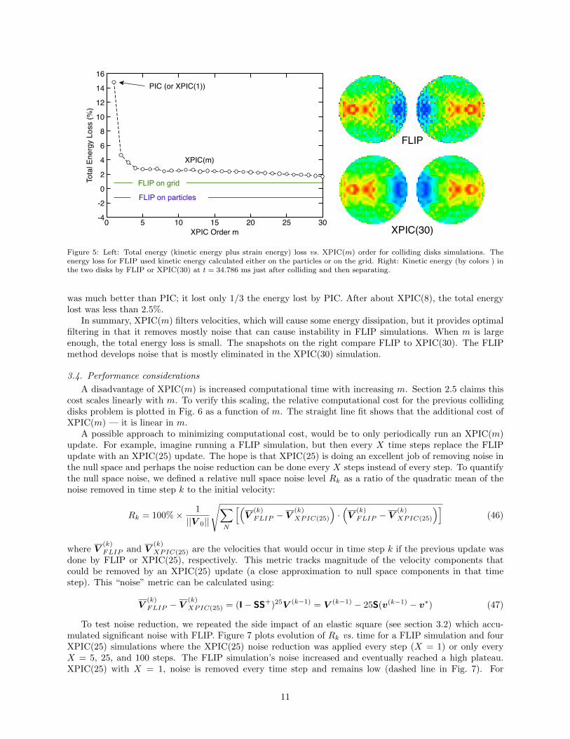
3.3. Two Colliding Disks

To examine energy conservation, we considered a simulation where two circular disks collide. The two,25 mm radius disks were modeled with a hyperelastic neohookean material [26] with E = 1 MPa, ν = 0.33,and ρ = 1 g/cm3. The background grid had 2× 2 mm cells, the time step was 0.026 ms, and uGIMP shapefunctions were used. The disks were moving towards each other with initial speed of 0.316 m/s (or 1% ofthe material’s wave speed). Contact between the disks was resolved explicitly using multimaterial MPMmethods based on both contact pressure and relative displacement of the two disks [25].

For an elastic impact, total energy (kinetic energy plus strain energy) should be conserved. MPM is closeto conservation, but is not perfect. The total energy lost in the simulations at t = 174 ms, which was aftercontact and bouncing apart, is plotted in Fig. 5 for FLIP and XPIC(m) as a function of m. For FLIP, thetotal energy measured on the particles (“FLIP on particles”) actually increased about 1.3%. This increasemay be caused by velocity noise that particularly affects kinetic energy calculations. The “FLIP on grid”line shows total energy loss where kinetic energy is evaluated on the grid during each time step instead offrom particle velocity. Energy conservation by this calculation shows about 0.8% loss. For XPIC(m), thePIC method (i.e., XPIC(1)) lost about 15% of the energy and provides an example of the PIC methodcausing too much damping. As m increased, the energy conservation improved significantly. Even XPIC(2)

10

XPIC Order m

Tota

l Ene

rgy

Loss

(%)

0 5 10 15 20 25 30 -4

-2

0

2

4

6

8

10

12

14

16

FLIP on particles

FLIP on grid

XPIC(m)

PIC (or XPIC(1))

FLIP

XPIC(30)

Figure 5: Left: Total energy (kinetic energy plus strain energy) loss vs. XPIC(m) order for colliding disks simulations. Theenergy loss for FLIP used kinetic energy calculated either on the particles or on the grid. Right: Kinetic energy (by colors ) inthe two disks by FLIP or XPIC(30) at t = 34.786 ms just after colliding and then separating.

was much better than PIC; it lost only 1/3 the energy lost by PIC. After about XPIC(8), the total energylost was less than 2.5%.

In summary, XPIC(m) filters velocities, which will cause some energy dissipation, but it provides optimalfiltering in that it removes mostly noise that can cause instability in FLIP simulations. When m is largeenough, the total energy loss is small. The snapshots on the right compare FLIP to XPIC(30). The FLIPmethod develops noise that is mostly eliminated in the XPIC(30) simulation.

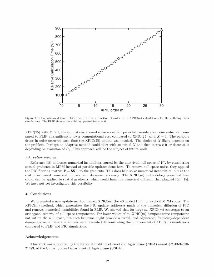
3.4. Performance considerations

A disadvantage of XPIC(m) is increased computational time with increasing m. Section 2.5 claims thiscost scales linearly with m. To verify this scaling, the relative computational cost for the previous collidingdisks problem is plotted in Fig. 6 as a function of m. The straight line fit shows that the additional cost ofXPIC(m) — it is linear in m.

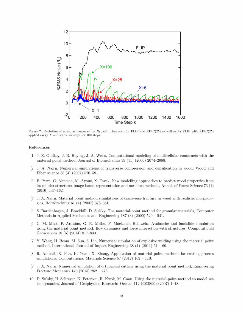
A possible approach to minimizing computational cost, would be to only periodically run an XPIC(m)update. For example, imagine running a FLIP simulation, but then every X time steps replace the FLIPupdate with an XPIC(25) update. The hope is that XPIC(25) is doing an excellent job of removing noise inthe null space and perhaps the noise reduction can be done every X steps instead of every step. To quantifythe null space noise, we defined a relative null space noise level Rk as a ratio of the quadratic mean of thenoise removed in time step k to the initial velocity:

Rk = 100%× 1

||V 0||

√∑N

[(V

(k)

FLIP − V(k)

XPIC(25)

)·(V

(k)

FLIP − V(k)

XPIC(25)

)](46)

where V(k)

FLIP and V(k)

XPIC(25) are the velocities that would occur in time step k if the previous update wasdone by FLIP or XPIC(25), respectively. This metric tracks magnitude of the velocity components thatcould be removed by an XPIC(25) update (a close approximation to null space components in that timestep). This “noise” metric can be calculated using:

V(k)

FLIP − V(k)

XPIC(25) = (I− SS+)25V (k−1) = V (k−1) − 25S(v(k−1) − v∗) (47)

To test noise reduction, we repeated the side impact of an elastic square (see section 3.2) which accu-mulated significant noise with FLIP. Figure 7 plots evolution of Rk vs. time for a FLIP simulation and fourXPIC(25) simulations where the XPIC(25) noise reduction was applied every step (X = 1) or only everyX = 5, 25, and 100 steps. The FLIP simulation’s noise increased and eventually reached a high plateau.XPIC(25) with X = 1, noise is removed every time step and remains low (dashed line in Fig. 7). For

11

XPIC order m

Rel

ativ

e C

alcu

latio

n Ti

me

(%)

0 5 10 15 20 25 30 0

100

200

300

400

500

600

700

800

900

Figure 6: Computational time relative to FLIP as a function of order m in XPIC(m) calculations for the colliding diskssimulations. The FLIP time is the solid dot plotted for m = 0.

XPIC(25) with X > 1, the simulations allowed some noise, but provided considerable noise reduction com-pared to FLIP at significantly lower computational cost compared to XPIC(25) with X = 1. The periodicdrops in noise occurred each time the XPIC(25) update was invoked. The choice of X likely depends onthe problem. Perhaps an adaptive method could start with an initial X and then increase it or decrease itdepending on evolution of Rk. This approach will be the subject of future work.

3.5. Future research

Reference [18] addresses numerical instabilities caused by the nontrivial null space of S+, by consideringspatial gradients in MPM instead of particle updates done here. To remove null space noise, they appliedthe PIC filtering matrix, P = SS+, to the gradients. This does help solve numerical instabilities, but at thecost of increased numerical diffusion and decreased accuracy. The XPIC(m) methodology presented herecould also be applied to spatial gradients, which could limit the numerical diffusion that plagued Ref. [18].We have not yet investigated this possibility.

4. Conclusions

We presented a new update method named XPIC(m) (for eXtended PIC) for explicit MPM codes. TheXPIC(m) method, which generalizes the PIC update, addresses much of the numerical diffusion of PICand removes numerical instabilities found in FLIP. We showed that for large m, XPIC(m) converges to anorthogonal removal of null space components. For lower values of m, XPIC(m) dampens some componentsnot within the null space, but such behavior might provide a useful, and adjustable, frequency-dependentdamping scheme. Several examples were presented demonstrating the improvement of XPIC(m) simulationscompared to FLIP and PIC simulations.

Acknowledgements

This work was supported by the National Institute of Food and Agriculture (NIFA) award #2013-34638-21483, of the United States Department of Agriculture (USDA).

12

Time Step k

%R

MS

Noi

se (R

k)

0 200 400 600 800 1000 1200 1400 1600 -2

0

2

4

6

8

10

12

FLIP

X=100

X=25

X=5

X=1

Figure 7: Evolution of noise, as measured by Rk, with time step for FLIP and XPIC(25) as well as for FLIP with XPIC(25)applied every X = 5 steps, 25 steps, or 100 steps.

References

[1] J. E. Guilkey, J. B. Hoying, J. A. Weiss, Computational modeling of multicellular constructs with thematerial point method, Journal of Biomechanics 39 (11) (2006) 2074–2086.

[2] J. A. Nairn, Numerical simulations of transverse compression and densification in wood, Wood andFiber science 38 (4) (2007) 576–591.

[3] P. Perre, G. Almeida, M. Ayouz, X. Frank, New modelling approaches to predict wood properties fromits cellular structure: image-based representation and meshless methods, Annals of Forest Science 73 (1)(2016) 147–162.

[4] J. A. Nairn, Material point method simulations of transverse fracture in wood with realistic morpholo-gies, Holzforschung 61 (4) (2007) 375–381.

[5] S. Bardenhagen, J. Brackbill, D. Sulsky, The material-point method for granular materials, ComputerMethods in Applied Mechanics and Engineering 187 (3) (2000) 529 – 541.

[6] C. M. Mast, P. Arduino, G. R. Miller, P. Mackenzie-Helnwein, Avalanche and landslide simulationusing the material point method: flow dynamics and force interaction with structures, ComputationalGeosciences 18 (5) (2014) 817–830.

[7] Y. Wang, H. Beom, M. Sun, S. Lin, Numerical simulation of explosive welding using the material pointmethod, International Journal of Impact Engineering 38 (1) (2011) 51 – 60.

[8] R. Ambati, X. Pan, H. Yuan, X. Zhang, Application of material point methods for cutting processsimulations, Computational Materials Science 57 (2012) 102 – 110.

[9] J. A. Nairn, Numerical simulation of orthogonal cutting using the material point method, EngineeringFracture Mechanics 149 (2015) 262 – 275.

[10] D. Sulsky, H. Schreyer, K. Peterson, R. Kwok, M. Coon, Using the material-point method to model seaice dynamics, Journal of Geophysical Research: Oceans 112 (C02S90) (2007) 1–18.

13

[11] A. Stomakhin, C. Schroeder, L. Chai, J. Teran, A. Selle, A material point method for snow simulation,ACM Trans. Graph. 32 (4) (2013) 102:1–102:10.

[12] J. A. Nairn, Material point method calculations with explicit cracks, Computer Modeling in Engineeringand Sciences 4 (6) (2003) 649–664.

[13] S. G. Bardenhagen, J. A. Nairn, H. Lu, Simulation of dynamic fracture with the material point methodusing a mixed J-integral and cohesive law approach, International Journal of Fracture 170 (1) (2011)49–66.

[14] F. Harlow, The particle in cell computing method for fluid dynamics, Methods in Computational Physics3 (1964) 319.

[15] J. U. Brackbill, H. M. Ruppel, FLIP: A method for adaptively zoned, particle-in-cell calculations offluid flows in two dimensions, Journal of Computational Physics 65 (2) (1986) 314 – 343.

[16] J. Brackbill, D. Kothe, H. Ruppel, FLIP: A low-dissipation, particle-in-cell method for fluid flow,Computer Physics Communications 48 (1) (1988) 25 – 38.

[17] D. Sulsky, Z. Chen, H. Schreyer, A particle method for history-dependent materials, Computer Methodsin Applied Mechanics and Engineering 118 (1) (1994) 179 – 196.

[18] C. Gritton, M. Berzins, R. M. Kirby, Improving accuracy in particle methods using null spaces andfilters, in: Proceedings of the 4th International Conference on Particle-Based Methods - Fundamentalsand Applications, PARTICLES 2015, International Center for Numerical Methods in Engineering, 2015,pp. 202–213.

[19] S. G. Bardenhagen, E. M. Kober, The generalized interpolation material point method, ComputerModeling in Engineering and Sciences 5 (6) (2004) 477–496.

[20] A. Sadeghirad, R. M. Brannon, J. Burghardt, A convected particle domain interpolation techniqueto extend applicability of the material point method for problems involving massive deformations,International Journal for Numerical Methods in Engineering 86 (12) (2011) 1435–1456.

[21] M. Steffen, P. C. Wallstedt, J. E. Guilkey, R. M. Kirby, M. Berzins, Examination and analysis ofimplementation choices within the material point method (MPM), Computer Modeling in Engineeringand Sciences 31 (2) (2008) 107–127.

[22] A. Ben-Israel, T. N. Greville, Generalized Inverses, Theory and Application, Springer-Verlag, New York,2003.

[23] L. N. Trefethen, D. Bau III, Numerical linear algebra, Vol. 50, Siam, 1997.

[24] S. G. Bardenhagen, J. E. Guilkey, K. M. Roessig, J. U. Brackbill, W. M. Witzel, J. C. Foster, Animproved contact algorithm for the material point method and application to stress propagation ingranular materials, Computer Modeling in Engineering and Sciences 2 (2001) 509–522.

[25] J. A. Nairn, Modeling of imperfect interfaces in the material point method using multimaterial methods,Computer Modeling in Engineering and Sciences 92 (3) (2013) 271–299.

[26] R. W. Ogden, Non-Linear Elastic Deformations, Dove Publications, Inc., Mineola, New York (page222), 1984.

14

Appendix

We derive some exact results for nearest-neighbor grid point (NGP) shape functions applied to problemswhere all particles have the same mass.

Theorem 1. If S is the matrix of NGP shape functions and all the particles have the same mass, then S isthe Moore-Penrose inverse of S+.

Proof. Consider S, it is a non-negative matrix created from nearest neighbor interpolations. By definition,each particle maps to only one grid point, so each row has only one nonzero element and it is equal to one.Consequentially, the columns of S are orthogonal and S can be into partitioned by its nonzero columns.Each column has the Moore-Penrose generalized inverse (denoted with †):

S†i = ||Si||−2STi (48)

Because all elements of Si are either 1 or 0:

S†i = (∑p

Si)−1STi (49)

Because the columns are orthogonal (i.e.. SiSTj = 0 for i 6= j), the Moore-Penrose inverse of S, or S†, is the

matrix of columns S†i . Thus for constant mass particles

S† = DST = S+ where D = diag

(∑p

Spi

)−1

(50)

By the properties of Moore-Penrose generalized inverses, (S+)† = (DST )† = S.

Theorem 2. If A is a linear map such that A : Rn → Rm with m < n, then the inverse problem:

x = argminx

‖x− x0‖2 such that : Ax = b (51)

has the solutionx = A†b+ (I −A†A)x0 (52)

where A† is the Moore-Penrose inverse of A.

Proof. Introduce Lagrange multipliers:

L(x, λ) = (x− x0)T (x− x0) + λT (Ax− b) (53)

Differentiating with respect to x and λ gives:

∇xL = 2(x− x0) +ATλ and ∇λL = Ax− b (54)

Setting ∇xL = ∇λL = 0 and solving for x gives:

x = AT (AAT )−1b−AT (AAT )−1Ax0 + x0 (55)

Because all elements of A are real, its Moore-Penrose inverse is A† = AT (AAT )−1 and Eq. (55) simplifies to:

x = A†b+ (I −A†A)x0 (56)

Theorem 3. If S+ represents the mapping matrix from the particles to grid and S represents the mappingfrom grid to particles, and all particles have the same mass, then

limm→∞

(I− SS+)m = Ω (57)

where Ω is an orthogonal projection onto the null space of S+.

15

Proof. The matrix (I − SS+) can be written as (I − SDST ). Decompose S using weighted singular valuedecomposition: S = UΣV T where U is an N × N orthogonal matrix, Σ is an N × n matrix containingsingular values of the matrix S on the main diagonal, and V is an n× n matrix that is orthonormal over itsconstraint, i.e. V TDV = I. Partition the decomposition by its non-zero singular values:

S =

[U1 U2

]Σr 0

0 0

V T1V T2

(58)

where Σr is a diagonal matrix with dimension of the rank of S. Solve for Σ:

Σ =

Σr 0

0 0

=

[UT1 UT2

]SD

[V1 V2

]=⇒

[UT1 SDV1 UT2 SDV2

]=

[0 0

]

=⇒ UT2 SDV1 = 0 and UT2 SDV2 = 0 =⇒ UT2 SD = 0

=⇒ DSTU2 = S+U2 = 0 (59)

So the matrix U2 forms an orthonormal basis for the null space of S+. Rewriting the matrix of interest:

(I− SS+)m = U1(1− Σ2r)mUT1 + U2U

T2 (60)

The matrix SS+ is a doubly stochastic matrix, so all its eigenvalues are ∈ [0, 1], the diagonal elements ofΣr ∈ (0, 1], and it follows that:

limm→∞

(1− Σ2r)m = 0 (61)

Finally, limm→∞

(I− SS+)m = U2UT2 , which is an orthogonal projection onto the null space of S+.

16