A New Method for Dealing with Measurement Error in Explanatory Variables of Regression Models

A New Method for Dealing with Measurement Error in Explanatory Variables of RegressionModelsAuthor(s): Laurence S. Freedman, Vitaly Fainberg, Victor Kipnis, Douglas Midthune andRaymond J. CarrollSource: Biometrics, Vol. 60, No. 1 (Mar., 2004), pp. 172-181Published by: International Biometric SocietyStable URL: http://www.jstor.org/stable/3695565 .

Accessed: 28/06/2014 19:09

Your use of the JSTOR archive indicates your acceptance of the Terms & Conditions of Use, available at .http://www.jstor.org/page/info/about/policies/terms.jsp

.JSTOR is a not-for-profit service that helps scholars, researchers, and students discover, use, and build upon a wide range ofcontent in a trusted digital archive. We use information technology and tools to increase productivity and facilitate new formsof scholarship. For more information about JSTOR, please contact [email protected].

.

International Biometric Society is collaborating with JSTOR to digitize, preserve and extend access toBiometrics.

http://www.jstor.org

This content downloaded from 91.223.28.163 on Sat, 28 Jun 2014 19:09:39 PMAll use subject to JSTOR Terms and Conditions

http://www.jstor.org/action/showPublisher?publisherCode=ibs

http://www.jstor.org/stable/3695565?origin=JSTOR-pdf

http://www.jstor.org/page/info/about/policies/terms.jsp


BIOMETRICS 60, 172-181 March 2004

A New Method for Dealing with Measurement Error in Explanatory Variables of Regression Models

Laurence S. Freedman,1'* Vitaly Fainberg,1 Victor Kipnis,2 Douglas Midthune,2 and Raymond J. Carroll3

1Department of Mathematics and Statistics, Bar Ilan University, Ramat Gan 52900, Israel

2Biometry Research Group, Division of Cancer Prevention, National Cancer Institute, MSC 7354, Bethesda, Maryland 20892-7354, U.S.A.

3Department of Statistics, Texas A&M University, College Station, Texas 77843-3143, U.S.A. * email: [email protected]

SUMMARY. We introduce a new method, moment reconstruction, of correcting for measurement error in covariates in regression models. The central idea is similar to regression calibration in that the values of the covariates that are measured with error are replaced by "adjusted" values. In regression calibration the adjusted value is the expectation of the true value conditional on the measured value. In moment reconstruction the adjusted value is the variance-preserving empirical Bayes estimate of the true value conditional on the outcome variable. The adjusted values thereby have the same first two moments and the same covariance with the outcome variable as the unobserved "true" covariate values. We show that moment reconstruction is equivalent to regression calibration in the case of linear regression, but leads to different results for logistic regression. For case-control studies with logistic regression and covariates that are normally distributed within cases and controls, we show that the resulting estimates of the regression coefficients are consistent. In simulations we demonstrate that for logistic regression, moment reconstruction carries less bias than regression calibration, and for case-control studies is superior in mean-square error to the standard regression calibration approach. Finally, we give an example of the use of moment reconstruction in linear discriminant analysis and a nonstandard problem where we wish to adjust a classification tree for measurement error in the explanatory variables.

KEY WORDS: Case-control study; Classification trees; Cohort study; Errors-in-variables; Linear discriminant analysis; Logistic regression; Measurement error; Regression calibration.

1. Introduction There is now a large literature on dealing with measurement error in the covariates of regression models (Fuller, 1987; Carroll, Ruppert, and Stefanski, 1995a; Cheng and Van Ness, 1999). The literature has become important in biostatistics, particularly epidemiology, because many important exposures are known to be measured imprecisely, and this imprecision can introduce serious bias into the estimates of regression coefficients and relative risks for these variables (Liu et al., 1978). Moreover, the statistical power of studies based on im- precise methods can be strongly affected by the imprecision (Freudenheim and Marshall, 1988).

One of the most popular methods for dealing with measurement error in covariates is regression calibration (Carroll and Stefanski, 1990; Gleser, 1990). The attraction of the method is its simplicity, both in concept and in practical implementation. The main idea is as follows. Suppose there is an outcome (dependent) variable Y related by a regression model to covariates X, and that we cannot observe X directly but observe W in its place, where W is X with some added error. Then, in order to estimate the regression coefficients, we

replace X with an estimate Xr, that is a function (defined in Section 2) of W. It can be shown that the method yields consistent estimates of / for linear regression, and that bias is often small for logistic regression (Carroll et al., 1995a, Chapter 3).

Despite the generally positive experience gained with using regression calibration, certain drawbacks have been noted. Perhaps the most serious of these are: (i) The method is only approximately consistent for nonlinear regression models.

(ii) The estimate Xrc does not in general preserve the variance-covariance structure of X. For example, in the sim- plest case of the "classical" measurement error model, where the error is additive and independent of X, the variance of Xrc, is always less than the variance of X. Thus, regression calibration requires substitution of values Xrc for X, even though, contrary to intuition, the distribution of Xrc does not approximate the distribution of X. Consequently, although re-

gression calibration is suitable for estimating regression coefficients, it is not suitable for estimating residual variances or other properties of the regression model. (iii) Regression calibration is valid only under the assumption of nondifferential

172



Explanatory Variables of Regression Models 173

measurement error, i.e., that the distribution of Wconditional on X and Y is equal to the distribution of W conditional on X.

In this article we introduce a method that, like regression calibration, involves substitution of an estimated value for X in the regression model, but in which the first and second moments of the substituted value are consistent estimates of the first and second moments of X. Because of this central property, we call the method "moment reconstruction."

One important advantage of the moment reconstruction approach is that it retains the simplicity of regression calibration, allowing use of standard software, while providing consistent estimation in nonlinear models, when covariates are normally distributed (see below). Other methods, such as corrected score methods (e.g., Huang and Wang, 2001) and full likelihood methods (e.g., Schafer, 1993), provide consistent estimation in more general situations, but require special- ized software for implementation. A second advantage of the method is that it enables direct estimation of other regression model parameters such as the residual variance or classification error rates (see our example). A third advantage of the method is that it remains valid under certain types of differential measurement error, unlike other methods currently proposed for use in nonlinear models.

In Section 2, we describe a motivating example and then propose the new method. In Section 3, we prove that the method gives exactly the same results as regression calibration for linear regression models. In Section 4, we prove that the method gives consistent estimates for the case of logistic regression in a case-control study where the covariate is normally distributed in each group. We then show, via simulation, that moment reconstruction carries less bias than regression calibration and has superior mean-squared error in large samples for logistic regression both in cohort and case- control study designs. In Section 5, we describe some extensions to the basic method. In Section 6, we demonstrate the use of the method in correcting a linear discriminant analysis for measurement error in its explanatory variables and also in the nonstandard problem of correcting a classification tree for measurement error. In Section 7, we summarize the main points of the article.

2. Example and Method Description 2.1 Example We wish to create a discriminant function for distinguishing between female carriers and noncarriers of Duchenne's muscular dystrophy mutation. The male offspring of female carriers who inherit the mutation are easily recognized as carriers and die early in life. The female offspring who inherit the mutation show no obvious signs of the mutation. No genetic test exists, but there are four biochemical markers: creatine kinase (CK), hemopexin (H), lactate dehydrogenase (LD), and pyru- vate kinase (PK). The discriminant function based on these four markers could then possibly be used to diagnose who is a carrier and who is not. These markers were measured on a group of 127 known noncarriers and 67 known carriers and the full data are presented in Andrews and Herzberg (1985, p. 223-228).

Estimating a discriminant function based on the four biochemical markers is a standard problem. However, the assays

for these markers are subject to day-to-day variation and lab- oratory error. Naturally, such error will affect the discriminatory power. Suppose that investigators consider that the discriminatory power using the error-prone measurements is insufficient and pose the following question: By how much would we improve the error rates in the classification procedure were we able to observe the "exact" values of the four markers for each individual? This might be of interest, for example, if they were able effectively to eliminate error from the measurement procedure, say, by taking many repeat measurements on each individual and using the means. The method of moment reconstruction, unlike regression calibration, may be used to directly estimate classification error rates under this hypothetical exact measurement scenario. In Section 6, we describe the application of the method to this problem. In the remainder of this section we describe the general method.

2.2 Basic Idea We assume the following general regression setup: a dependent variable Y (an n x 1 vector) is related to covariates X (an n x p matrix) according to

E(Y I X, ) = f(X, /), (1)

for some unknown parameter /3. Suppose X is measured with error and W is observed. In regression calibration we substitute the conditional expectation of X on W, Xrc(W) E(X I W), and run the regression model

E(Y I W, P) %f {Xrc(W), 3} . (2)

For the new method we will first assume measurement error in X such that

E(W I Y) = E(X I Y). (3)

In other words, we consider the case where W is an unbiased measurement of X: This condition can be relaxed (see Section 2.7).

The main aim of moment reconstruction is to substitute, in place of the observed W, values that have the same joint distribution with Y as (X, Y). Clearly inasmuch as the substituted values will have the same distribution as X and will have the same joint distribution with Yas (X, Y), the method will consistently estimate all parameters that are consistently estimated by (X, Y) data. In the general case, finding the correct substitution is a very difficult problem, but if we content ourselves with the lesser aim of matching just the first two moments of the joint distribution, then a simple solution can be obtained.

As we will prove in Section 2.3, the solution is given by

Xmr(W, Y) = E(W I Y)(I - G) + WG, (4)

where the p x p matrix G = G(Y) = {cov(W y)I/2}-1 cov(X Y)1/2 and A1/2 is the Cholesky decomposition of A defined by (A1/2)TA1/2 = A. The idea of moment reconstruction is to substitute Xmr(W, Y) for X in the regression model (1), and thus to estimate /3 via the regression model

E(Y I W, P3) f {Xmr(W, Y), /P} . (5)



174 Biometrics, March 2004

2.3 First Two Moments of Xmr and X Are Equal Given Y

In the rest of the article we will write Xmr(W, Y) as Xmr for short. We now show that (Xmr, Y) has the same first and second moments as (X, Y), and indeed more crucially that Xmr and X have the same first and second moments conditional on Y.

The first moment is obvious from (3): E(XmrIY) - E(W I Y) (I - G) + E(W I Y)G = E(W I Y) = E(XIY). For the second moment, note that from (4),

cov(Xmr IY) = GTcov(W I Y)G = {cov(X Y)l/2}T{cov(W I )1/2}-1)T

x cov(W I Y){cov(W I y)1/2-1cov(X I Y)1/2

= {cov(X I Y)1/2}TCov(X Y)1/2 = COv(X I Y),

as claimed. This of course means that the unconditional second moments of Xmr and X are the same, as well as

cOV(Xmr, Y) = cov(X, Y).

2.4 Implications

Using the result in Section 2.3, it is clear that if (X, Y) and

(W, Y) both have multivariate normal distributions, then

(Xmr, Y) is also multivariate normal and has the same distribution as (X, Y), since these distributions are defined com- pletely by their first and second moments.

Now consider the case where Y has any distribution and the conditional distributions [X I Y] and [W I Y] are both multivariate normal for each value of Y. Then since, in the proof of Section 2, we showed that the first two moments of [Xmr I Y] are the same as those of [X I Y], it follows that they have the same distribution, as do (Xmr, Y) and (X, Y).

2.5 Implementation In the implementation of the method, to compute Xmr from equation (4), one substitutes estimates for E(W I Y) and G =

G(Y) to obtain Xmr. As long as these estimates are consistent, it is clear that (Xmr, Y) will preserve asymptotically the first and second moments of (X, Y). Thus, statistical procedures that involve only the first and second moments of the variables X and Y, should, intuitively, perform well under substitution of Xmr for X. If, in addition, the normality assumptions on

[X I Y] and [W I Y] hold, then it is also clear that identical functions of (Xmr, Y) and (X, Y) will have the same asymp- totic limits, e.g., for parameter estimates, error rates, etc. We will use this fact in Section 6, in an example where Y is a binary variable.

The method of estimation of E(W Y) and G = G(Y) will depend on the specific regression models for Y on X, on the measurement error model, and on the type of substudy that is conducted to provide information on the measurement error in W. Here, to provide a flavor, we give an example. Suppose that in the main study we observe (Wi, Yi), i = 1, 2,... , n, and in an independent substudy (on other subjects) we observe

(Wlj, W2j), j = 1, 2,..., m. Here, Wis a vector of p covariates and Y has a multinomial distribution on k categories. The measurement error model is classical and nondifferential with all errors independent of X and mutually independent. Then E(W IY) is estimated from the main study by the mean of W within each category of Y. The estimated variance of the error

U in W, c6&(U), is obtained from the substudy, taking half of the sample covariance matrix of the differences Wlj - W2j. Since the model specifies zero covariance between the errors, we estimate just the p diagonal elements of this matrix. The estimated covariance matrices, c'(W I Y), of W conditional on Y are obtained from the main study, using the sample covariance matrices computed within each category of Y. The estimated covariances of X conditional on Y are then obtained from co5(W I Y) - cOv(U).

In each situation the procedure for estimating E(W IY) and G needs to be specified, so as to fully define Xmr. Further examples will be given in later sections.

2.6 Intuitive Meaning of Xmr

To appreciate the main differences between the Xrc of regression calibration and Xmr of moment reconstruction, consider the case of a single covariate X, and the classical measurement error model. In that case, Xrc is a weighted average of the unconditional expectation of W and the observed value of W, where the weight on W is the ratio of variances of X to W. In the same case, Xmr is a weighted average of the expectation of W conditional on Y and the observed value of W, where the weight on W is the ratio of the standard deviations of X to W conditional on Y. The conditioning on Y is an important feature of the method and allows substitution of an Xmr that preserves both the first and second moments of X and, simultaneously, the covariances of X with Y. One may think of Xmr as a variance-preserving empirical Bayes estimate of X, shrinking the observed value W back toward its expectation conditional on Y, where the amount of shrinkage depends on the amount of measurement error variance relative to the variance of X conditional on Y.

2.7 Biased Measurements In the definition of Xmr above we assumed in (3) that E(W I Y) = E(X I Y), i.e., that W is unbiased for X. Moment reconstruction is easily generalized to a case of known linear bias, that is, where E(W I Y) = a(Y) + b(Y)E(X I Y) with a(Y) and b(Y) known vector functions of Y. However, we will not pursue this modification in the rest of this article. We now explore the properties of moment reconstruction in different regression models.

3. Linear Regression The purpose of this section is to show that in linear regression, moment reconstruction reduces to the usual correction for at- tenuation, i.e., the regression calibration estimate. We make no assumptions about normality. Consider linear regression with the classical measurement error model

Y = /3o + XT3 + e, (6)

w=x+u, (7)

where (X, e, U) are independent, X has mean 1x and covariance matrix Exx and (U, e) have mean zero and variances

Et and ao, respectively. Using (7), the covariance matrix of W is EZ,, = EX +

Euu. Without loss of generality we may as-

sume that the sample means of Y and W have mean zero and we will ignore the intercept. Also, we will assume that

Yu is

known. Let E,, be the usual sample covariance matrix of the W's, except division is by n rather than n - 1. In a sample




of size n, this means that the ordinary regression calibration estimate is given as Orc = (Eww - Euu)-ln- 1 WYi.

For moment reconstruction the relevant quantities are the following:

E = Ew - UU

E(WIY)-=YZYYW ZY2 i=1 i=1

c T(W Y) =n-1 W( - WZTYiWiYi 2 ,

i=1 i=1 i=1 / i=1

c•y(X | Y) = n- T- n- Wi YE W

Yi Yi

i=1 i=1 i=1

Define Xmr,i = E(WIY)(I - G) + WIG, where G = {c-v(W Iy)1/2 -1ov(X Y)1/2. Then our estimate of /3 is given by /mr

= ( i=l Xmr,iXmr,i)-

(Z X= i It is an easy but tedious calculation to show that

n-1 Xm rXmr,iZ = Ex, and that n-1i=1 Xmr,ii =

n-1

•.i

W7Yj. Hence, moment reconstruction equals regression calibration in linear regression.

It is worth pointing out that moment reconstruction has an added benefit in this model, in the case that the main study and the substudy sample sizes both become large. In this case, moment reconstruction yields a consistent estimate of the regression error variance a., something that regression calibration does not do. This is because (X, Y) and (Xmr, Y) have the same covariance matrix.

4. Logistic Regression Let the outcome Y be binary (0 or 1) and let X be the explanatory variable. We consider logistic regression models of the form Pr(Y = 1) = H(Oo + XTp), where H(v) =

{1 + exp(-v)}-1 is the logistic distribution function. We assume that among the controls, i.e., Y - 0,

X = Normal(to, Exx). It may be shown (Carroll, Wang, and Wang, 1995b) that among the cases, i.e., Y = 1, X is also normally distributed: X = Normal(po + Exx, Exx). Hence, [X IY = y] = Normal(io + Exx3y, EZ).

Two versions of this problem exist: In the first version (cohort design), a given number of individuals are randomly sampled from a single population containing cases and controls, and Y is observed on these individuals. In the second version (case-control design), a given number of individuals are randomly sampled separately from the populations of cases

(Y = 1) and controls (Y = 0). It has been shown (Carroll et al., 1995b, Section 3.9) that in

the cohort and case-control versions of this model, regression calibration is approximately but not exactly consistent for logistic regression. However the implementation of regression calibration for these two versions is different. In the cohort version, regression calibration is performed in the usual man- ner, deriving the expression for E(X IW) from a substudy carried out on a random sample from the same population as the main study, or from a population as similar to it as pos- sible. In the case-control version the expression for E(X I W) must be derived from a random sample of controls, not cases,

on the assumption that the disease is rare (Carroll et al., 1995b).

In this section, we will first show that moment reconstruction is consistent for 3 in either version of this model. We will then describe a simulation experiment comparing regression calibration and moment reconstruction for the case-control version of this model, and also for a second model to be described.

4.1 Consistency of Moment Reconstruction for Estimating /3 We now show that moment reconstruction yields consistent estimates of /3 in either the case-control or cohort settings when X and W given Y are multivariate normal.

We assume that the classical measurement error model (7) holds, although we allow for the possibility of differential measurement error by allowing the variance of the measurement error to depend on Y, so that W = X + U, where [U I Y = y] = Normal(0, E,,y). Because of the classical error model, [W IY = y] = Normal(po + EZxO, ZE +

EuU,y). Let Exx be a consistent estimate of E, which in the model

above is the variance of X conditional on Y, for both values of Y. In the case-control study design, this estimate can be constructed by computing the within case/control status sample covariance matrix of the W's, subtracting from it E,Z,, (obtained from an independent substudy involving repeated measurements of W), and then taking a weighted average of the two resulting estimates according to the number of cases and controls. A similar method can be used in the cohort study. Define GY - (ExZ

+ Eu

,y)-1/2 1/2. Furthermore,

define E(W I Y) as the mean of W within cases and controls, respectively. These definitions specify the meaning of Xmr = E(WI|Y)(I -

Gy) + WGy. Since Xmr = Xmr(Y, W) is

a (uniformly) consistent estimate of Xmr = Xmr(Y, W), and

since (Xmr, Y) and (X, Y) have the same joint distributions, this means moment reconstruction leads to consistent estimates of /3 in either case-control or cohort sampling.

Note that the above proof includes the case where the error variances depend on Y. Thus moment reconstruction is shown to be consistent also in a case where the error is differential.

4.2 Description of Simulation Studies We performed simulations of several different scenarios for logistic regression with normally distributed covariates. The scenarios included the following:

(1) Two models (i.e., distributions of covariates X): the case-control version of the model described in Sec- tion 4.1, where X is normally distributed among cases and controls; and a cohort design with X having a marginal normal distribution across the total population (Y = 0 and Y = 1 combined). The second model represents a modest departure from the assumptions made in our proof of consistency, and may be considered as a first enquiry into the robustness of moment reconstruction.

(2) Total sample sizes of 500, 1000, and in some cases 2000. (3) Parameters defining the precise model. (4) One or two covariates. The intercept was fixed at zero

for the case-control design and at -1.5 or -3.0 for the cohort design. The coefficients of the other X variables were fixed at 1.0 throughout.




(5) The correlation between the X covariates was fixed at 0.5. The variance of each [X IY] was fixed at 1.0 throughout.

(6) Generally we consider cases with substantial measurement error, between one to two times larger than the true variance of the variable. Errors of this magnitude often occur in epidemiology, particularly when mea- suring dietary intake (Liu et al., 1978). Variances of

[U IY] were therefore chosen as 1.0 or 2.0. Correlations between the U variables of 0.0, 0.5, or 0.8 were chosen. Some scenarios of the case-control design included different variances of U according to the value of Y

(differential error). We do not report results of differential error in the cohort design, as it is less likely to occur. The exact combinations of the parameters used are presented in Section 4.4.

Every scenario was simulated 400 times. In our simulations we used the following eight methods to estimate /.

T: True method, logistic regression of Y on X: This was included to measure the bias in the regression estimates arising from maximum likelihood with the finite sample sizes considered in this study.

U: Unadjusted method, logistic regression of Yon W. RC: Usual regression calibration, where E(X W) is

derived from a substudy in the total population. RC-F: Usual regression calibration modified by an ad-

justment similar to that proposed by Fuller (1987), which we explain below.

CRC: Control group regression calibration, where

E(X I W) is derived from a substudy among the population of controls.

CRC-F: Control group regression calibration with the Fuller-type adjustment.

MR: Moment reconstruction, with Xmr defined as in Section 4.1, except that we assume that the error variance is known rather than estimated, as explained below.

MR: Moment reconstruction with the Fuller-type adjustment.

In all methods that use an estimate of the error variance, i.e., all except T and U, we assume that the error variances are known exactly. We do not simulate the results of substudies from which the error variances may be estimated. For simulations of models with just one covariate, the three methods with the Fuller-type adjustment were not investigated. For the simulations of models with two covariates, all eight methods were investigated.

4.3 The Fuller-Type Adjustment Both regression calibration and moment reconstruction require estimation of Ex, which, as explained in Section 4.1, is given by the difference between the two variance estimators

E,, - E,,. Unfortunately, this difference is sometimes not positive-definite, and this can cause severe problems in estimating p/3. We used an adjustment similar to that described by Fuller (1987), so as to stabilize the estimation in these circumstances. Let A be the smallest root of the determinant equation det(E,, - AE,,) = 0. Then the adjusted estimator

of Exx is given by Exx = rxx + 6E,,/(n - 1), where n is the

sample size, and

EWW - EUU if A > n/(n - 1), rxx=

-

_{A- 6/(n

- 1)}Euu if A? n/(n -1).

We apply this adjustment to both versions of regression calibration and also to the estimates of conditional variance cov(X I Y) required in moment reconstruction.

4.4 Simulation Results

4.4.1 Case-control design: univariate model. Table 1 shows the mean estimate for the single covariate, its empirical

Table 1 Simulation results for case-control design: univariate modelsa

with nondifferential and differential measurement error

Errorb n V(u)c T U RC CRC MR

ND 500 1 /3 1.00 0.51 0.91 1.03 1.03 SE 0.11 0.07 0.14 0.20 0.18 RMSE 0.11 0.51 0.17 0.20 0.19

2 p/3 1.01 0.34 0.89 1.07 1.06 SE 0.11 0.06 0.18 0.33 0.29 RMSE 0.11 0.67 0.22 0.33 0.29

1000 1 31 1.00 0.50 0.90 1.02 1.01 SE 0.08 0.05 0.10 0.14 0.13 RMSE 0.08 0.50 0.14 0.14 0.13

2 p, 1.01 0.33 0.86 1.02 1.00 SE 0.08 0.04 0.12 0.21 0.18 RMSE 0.08 0.67 0.19 0.21 0.18

2000 1 31 1.00 0.50 0.90 1.01 1.01 SE 0.06 0.03 0.06 0.09 0.08 RMSE 0.06 0.50 0.12 0.09 0.08

2 p3 1.00 0.33 0.87 1.03 1.01 SE 0.06 0.03 0.09 0.15 0.12 RMSE 0.06 0.67 0.15 0.15 0.13

D 500 1,2 /3 1.00 0.40 0.88 0.82 1.01 SE 0.11 0.06 0.15 0.16 0.21 RMSE 0.11 0.60 0.19 0.24 0.21

2,1 31 1.01 0.41 0.90 1.30 1.04 SE 0.12 0.06 0.17 0.43 0.24 RMSE 0.12 0.61 0.20 0.52 0.25

1000 1,2 P/3 1.00 0.40 0.89 0.81 1.01 SE 0.08 0.04 0.11 0.11 0.15 RMSE 0.08 0.60 0.16 0.22 0.15

2,1 P/3 1.01 0.41 0.90 1.27 1.03 SE 0.08 0.05 0.12 0.29 0.17 RMSE 0.08 0.60 0.16 0.39 0.17

2000 1,2 31 1.01 0.40 0.89 0.81 1.01 SE 0.05 0.03 0.08 0.08 0.11 RMSE 0.05 0.61 0.14 0.21 0.11

2,1 3 1.00 0.40 0.88 1.22 1.00 SE 0.06 0.03 0.08 0.19 0.11 RMSE 0.06 0.60 0.14 0.29 0.11

alntercept = 0; /3 = 1.0; for meaning of T, U, RC, CRC, and MR, see Section 4.2.

bND, nondifferential; D, differential.

CFor differential error: V(uI Y= 0), V(uI Y= 1).




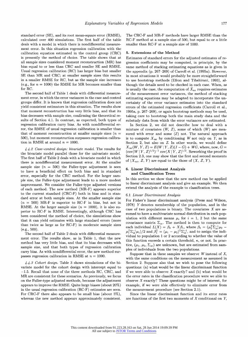
standard error (SE), and its root mean-square error (RMSE), calculated over 400 simulations. The first half of the table deals with a model in which there is nondifferential measurement error. In this situation regression calibration with the calibration equation estimated in the control group (CRC) is presently the method of choice. The table shows that at all sample sizes considered moment reconstruction (MR) has bias equal to or less than CRC and smaller SE and RMSE. Usual regression calibration (RC) has larger bias but smaller SE than MR and CRC; at smaller sample sizes this results in a smaller RMSE for RC, but as the sample size increases

(e.g., for n = 1000) the RMSE for MR becomes smaller than for RC.

The second half of Table 1 deals with differential measurement error, in which the error variances in the case and control groups differ. It is known that regression calibration does not yield consistent estimators in this situation. The results show that moment reconstruction has very little bias, and that its bias decreases with sample size, confirming the theoretical results of Section 4.1. In contrast, as expected, both types of regression calibration carry bias. As with nondifferential error, the RMSE of usual regression calibration is smaller than that of moment reconstruction at smaller sample sizes (n =

500), but moment reconstruction surpasses regression calibration in RMSE at around n = 1000.

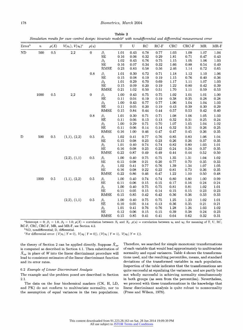
4.4.2 Case-control design: bivariate model. The results for the bivariate model parallel those for the univariate model. The first half of Table 2 deals with a bivariate model in which there is nondifferential measurement error. At the smaller sample size (n = 500) the Fuller-type adjustment is seen to have a beneficial effect on both bias and in standard error, especially for the CRC method. For the larger sample size, the Fuller-type adjustment leads to a more modest improvement. We consider the Fuller-type adjusted versions of each method. The new method (MR-F) appears superior to the current standard (CRC-F) both in bias and in standard error at both sample sizes. At the smaller sample size

(n = 500) MR-F is superior to RC-F in bias, but not in RMSE. At the larger sample size (n = 1000), it is also superior to RC-F in RMSE. Interestingly, although CRC has been considered the method of choice, the simulations show that it can yield estimates with large standard errors (more than twice as large as for RC-F) in moderate sample sizes

(e.g., 500). The second half of Table 2 deals with differential measure-

ment error. The results show, as in Table 1, that the new method has very little bias, and that its bias decreases with sample size, and that both types of regression calibration carry bias. As with nondifferential error, the new method surpasses regression calibration in RMSE at n = 1000.

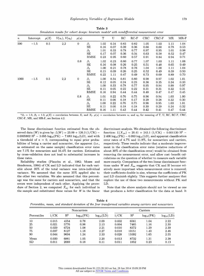
.~4.3 Cohort design. Table 3 shows simulations of the bivariate model for the cohort design with intercept equal to -1.5. Recall that none of the three methods RC, CRC, and MR are consistent for these scenarios. As previously, we focus on the Fuller-type adjusted methods, because the adjustment appears to improve the RMSE. Quite large biases (about 20%) in the usual regression calibration (RC-F) estimates are seen. For CRC-F there also appears to be small bias (about 5%), whereas the new method appears approximately consistent.

The CRC-F and MR-F methods have larger RMSE than the RC-F method at a sample size of 500, but equal to or a little smaller than RC-F at a sample size of 1000.

5. Extensions of the Method Estimates of standard errors for the adjusted estimates of regression coefficients may be computed, in principle, by the same method of stacking estimating equations as is given in the appendix (p. 267-269) of Carroll et al. (1995a). However, in most situations it would probably be more straightforward to use bootstrap methods (Efron and Tibshirani, 1993), although the details need to be checked in each case. When, as is usually the case, the computation of Xmr requires estimates of the measurement error variances, the method of stacking estimating equations may be adapted to incorporate the un- certainty of the error variance estimates into the standard errors of the estimated regression coefficients (Carroll et al., 1995a, p. 267-269), or again bootstrap methods may be used, taking care to bootstrap both the main study data and the substudy data from which the error variances are estimated.

In Section 2, we did not describe how to deal with a mixture of covariates (W, Z), some of which (W) are measured with error and some (Z) not. The natural approach is to compute Xmr by conditioning W not only on Y, as in Section 2, but also on Z. In other words, we would define

Xmr(W, Y, Z) = E(W I Y, Z)(I - G) + WG, where, now, G =

(cov(W I Y, Z)1/2)-1 cov(X I Y, Z)1/2. Reworking the proof in Section 2.3, one may show that the first and second moments of (Xmr, Z, Y) are equal to the those of (X, Z, Y).

6. Linear Discriminant Analysis and Classification Trees

In this section we show that the new method can be applied to linear discriminant analysis and give an example. We then extend the analysis of the example to classification trees.

6.1 Linear Discriminant Analysis For Fisher's linear discriminant analysis (Press and Wilson, 1978) Y denotes membership of the population, and in the case of two populations is binary. The covariates X are assumed to have a multivariate normal distribution in each population with different means pi for i = 1, 2 but the same covariance matrix Ex. The method is then to compute for each individual L(X) = • o +

X1l, where

/0 _ (TExx-z 2 -

lT1X1A)//2 and 3T = (L1 -

P.2)TX , and to assign the indi-

vidual to population 1 or 2 according to whether the value of this function exceeds a certain threshold, n, or not. In prac- tice, (Al, I2, Exx) are unknown, but are estimated from samples of individuals from the two populations.

Suppose that in these samples we observe W instead of X, with the same conditions on the measurement as assumed in Section 2. Suppose also that we wish to pose the following questions: (a) what would be the linear discriminant function if we were able to observe X exactly? and (b) what would be the error rates in the classification procedure were we able to observe X exactly? These questions might be of interest, for example, if we were able effectively to eliminate error from the measurement procedure (see Section 2.1).

Since the linear discriminant function and its error rates are functions of the first two moments of X conditional on Y,




Table 2 Simulation results for case-control design: bivariate modelsa with nondifferential and differential measurement error

Errorb n p(X) V(Ul), V(U2)c p(u) T U RC RC-F CRC CRC-F MR MR-F

ND 500 0.5 2,2 0 O1 1.01 0.43 0.78 0.77 1.03 1.09 1.07 1.04 SE 0.16 0.06 0.32 0.29 1.81 0.71 0.47 0.43 32 1.02 0.43 0.76 0.75 1.15 1.05 1.06 1.03 SE 0.16 0.07 0.34 0.32 1.66 0.88 0.54 0.49 RMSE 0.23 0.83 0.58 0.56 2.46 1.14 0.72 0.65

0.8 O1 1.01 0.30 0.72 0.71 1.18 1.12 1.10 1.06 SE 0.15 0.08 0.19 0.19 1.15 0.76 0.40 0.36 32 1.01 0.29 0.70 0.69 1.17 1.11 1.07 1.03 SE 0.15 0.09 0.20 0.19 1.22 0.80 0.42 0.39 RMSE 0.21 1.02 0.50 0.51 1.70 1.11 0.59 0.53

1000 0.5 2,2 0 Pl 1.00 0.43 0.75 0.75 1.02 1.01 1.01 1.00 SE 0.11 0.04 0.19 0.19 0.38 0.35 0.28 0.28 32 1.00 0.43 0.77 0.77 1.06 1.04 1.04 1.03 SE 0.11 0.05 0.20 0.19 0.43 0.39 0.30 0.29 RMSE 0.15 0.84 0.44 0.44 0.57 0.53 0.42 0.40

0.8 01 1.01 0.30 0.71 0.71 1.08 1.06 1.05 1.03 SE 0.11 0.06 0.13 0.13 0.32 0.31 0.25 0.24

/32 1.00 0.29 0.71 0.70 1.07 1.05 1.04 1.02 SE 0.11 0.06 0.14 0.14 0.32 0.31 0.26 0.25 RMSE 0.16 1.00 0.46 0.47 0.47 0.45 0.36 0.35

D 500 0.5 (1,1), (2,2) 0.5 31 1.02 0.41 0.77 0.76 0.85 0.83 1.06 1.04 SE 0.15 0.08 0.23 0.23 0.26 0.26 0.37 0.35

/32 1.01 0.40 0.74 0.74 0.82 0.80 1.03 1.01 SE 0.16 0.08 0.23 0.22 0.24 0.24 0.37 0.35 RMSE 0.22 0.87 0.49 0.49 0.44 0.44 0.52 0.50

(2,2), (1,1) 0.5 31 1.00 0.40 0.75 0.75 1.35 1.31 1.04 1.02 SE 0.15 0.08 0.21 0.20 0.77 0.70 0.35 0.33 32 1.02 0.41 0.77 0.76 1.39 1.34 1.07 1.05 SE 0.16 0.08 0.22 0.22 0.81 0.73 0.36 0.35 RMSE 0.22 0.86 0.46 0.47 1.22 1.10 0.50 0.48

1000 0.5 (1,1), (2,2) 0.5 01 1.00 0.40 0.74 0.74 0.80 0.80 1.00 0.99 SE 0.11 0.06 0.15 0.15 0.17 0.16 0.24 0.24 32 1.00 0.40 0.75 0.75 0.81 0.81 1.02 1.01 SE 0.11 0.05 0.15 0.14 0.15 0.15 0.23 0.23 RMSE 0.15 0.85 0.42 0.42 0.36 0.36 0.33 0.33

(2,2), (1,1) 0.5 31 1.00 0.40 0.75 0.75 1.25 1.23 1.02 1.01 SE 0.10 0.05 0.14 0.13 0.36 0.35 0.21 0.21

32 1.01 0.41 0.76 0.76 1.28 1.26 1.03 1.02 SE 0.12 0.06 0.15 0.15 0.39 0.38 0.24 0.23 RMSE 0.15 0.85 0.41 0.41 0.64 0.62 0.32 0.31

aIntercept = 0; 31 = 1.0, 32 = 1.0; p(X) = correlation between X1 and X2. p(u) = correlation between ul and u2; for meaning of T, U, RC, RC-F, CRC, CRC-F, MR, and MR-F, see Section 4.2.

bND, nondifferential; D, differential.

CFor differential error: ( V(ul I Y = 0), V(u2 I Y = 0)), ( V(ul I Y = 1), V(u2 I Y= 1)).

the theory of Section 2 can be applied directly. Suppose Xmr is computed as described in Section 4.1. Then substitution of

)mr in place of W into the linear discriminant procedure will

lead to consistent estimates of the linear discriminant function and its error rates.

6.2 Example of Linear Discriminant Analysis The example and the problem posed are described in Section 2.1.

The data on the four biochemical markers (CK, H, LD, and PK) do not conform to multivariate normality, nor to the assumption of equal variances in the two populations.

Therefore, we searched for simple monotonic transformations of each variable that would lead approximately to multivariate normality and equal variances. Table 4 shows the transformations used, and the resulting percentiles, means, and standard deviations of the transformed variables in each population. Inspection of the table indicates that the transformations are quite successful at equalizing the variances, and are partly but not wholly successful in achieving normality simultaneously in both groups (as seen from the percentiles). Nevertheless, we proceed with these transformations in the knowledge that linear discriminant analysis is quite robust to nonnormality (Press and Wilson, 1978).




Table 3 Simulation results for cohort design: bivariate modelsa with nondifferential measurement error

n Intercept p(X) V(Ul), V(u2) p(u) T U RC RC-F CRC CRC-F MR MR-F

500 -1.5 0.5 2,2 0 PI 1.02 0.34 0.83 0.82 1.05 1.03 1.11 1.04 SE 0.16 0.07 0.39 0.36 0.66 0.60 0.78 0.53 02 1.01 0.33 0.78 0.77 0.97 0.95 1.01 0.98 SE 0.17 0.07 0.36 0.34 0.63 0.58 0.52 0.47 RMSE 0.23 0.95 0.60 0.57 0.91 0.84 0.94 0.71

0.8 31 1.02 0.23 0.80 0.77 1.07 1.03 1.11 1.06 SE 0.16 0.08 0.26 0.25 0.51 0.48 0.65 0.49 02 1.00 0.21 0.78 0.76 1.04 1.00 1.11 1.04 SE 0.15 0.09 0.26 0.25 0.52 0.49 0.59 0.50 RMSE 0.22 1.11 0.47 0.49 0.73 0.69 0.89 0.70

1000 -1.5 0.5 2,2 0 /1 1.00 0.34 0.81 0.80 0.98 0.97 1.02 1.01 SE 0.12 0.05 0.24 0.23 0.36 0.35 0.34 0.33 02 1.00 0.33 0.78 0.77 0.95 0.94 0.99 0.97 SE 0.11 0.05 0.22 0.22 0.31 0.31 0.32 0.31 RMSE 0.16 0.94 0.44 0.44 0.48 0.47 0.47 0.45

0.8 13 1.01 0.22 0.76 0.75 0.96 0.94 1.03 1.00 SE 0.11 0.06 0.18 0.17 0.29 0.28 0.32 0.30 02 1.00 0.22 0.76 0.75 0.96 0.95 1.03 1.01 SE 0.11 0.06 0.18 0.18 0.30 0.29 0.34 0.32 RMSE 0.16 1.11 0.43 0.44 0.42 0.41 0.47 0.44

a•1 = 1.0, /2 = 1.0; p(X) = correlation between X1 and X2. p(u) = correlation between

u, and u2; for meaning of T, U, RC, RC-F, CRC,

CRC-F, MR, and MR-F, see Section 4.2.

The linear discriminant function estimated from the observed data (W) is given by: L(W) = 23.09 + 126.3 (1/CK) - 0.0005802 H2 - 3.095 logio(PK) - 7.683 loglo(LD), and with a threshold of

,, = 0, corresponding to equal prior proba-

bilities of being a carrier and noncarrier, the apparent (i.e., as estimated on the same sample) classification error rates are 7.1% for noncarriers and 16.4% for carriers. Estimation by cross-validation does not lead to substantial increases in these rates.

Reliability studies (Plauchu et al., 1982; Moses and Henderson, 1984) of CK and LD indicated that for each variable about 35% of the total variance was intra-individual variance. We assumed that the same 35% applied also to the other two variables. We also assumed that this percent- age was the same for carriers and noncarriers, and that the errors were independent of each other. Applying the procedure of Section 2, we computed Xmr for each individual in the sample and substituted these values for W in the linear

discriminant analysis. We obtained the following discriminant function: L(Xmr) = 20.41 + 243.1 (1/CK) - 0.001130 H2 - 2.406 loglo(PK) - 6.083 loglo(LD), and apparent classification error rates of 4.7% and 11.9%, for noncarriers and carriers, respectively. These results indicate that a moderate improvement in the classification error rates (relative reductions of about 30% of the classification error) would be obtained from removing the measurement error, and allow cost-benefit cal- culations on the question of whether to measure each variable more exactly. Comparison of the two linear discriminant functions under W and Xmr suggests that CK and H become rel- atively more important when measurement error is removed; their coefficients double in size, whereas the coefficients of PK and LD diminish slightly. This suggests further analyses that explore the use of these two measurements without PK and LD.

Note that the above analysis should not be viewed as one that produces a better classification for the data at hand. It

Table 4 Percentiles, mean, and standard deviation of the four transformed variables among carriers and noncarriers

Noncarriers Carriers

Percentiles 1/CK H2 log0o(PK) loglo(LD) 1/CK H2 log0o(PK) loglo(LD)

10 0.015 4554 0.78 2.09 0.002 6561 1.04 2.22 25 0.021 5776 0.98 2.13 0.004 7465 1.16 2.30 50 0.029 6724 1.08 2.21 0.010 8372 1.29 2.39 75 0.037 8127 1.18 2.27 0.018 10151 1.40 2.46 90 0.044 9604 1.24 2.33 0.028 11092 1.65 2.55 Mean 0.030 6881 1.05 2.20 0.013 8732 1.31 2.38 SD 0.011 2069 0.18 0.11 0.011 1852 0.23 0.13




Y N LD<232.5

y N C:40 S NC:4

CK<98.2 Pr : 0.91

C:8

NC : 1 Y N

Pr: 0.89 iH<l00.0

C: 11 N Y NC : 113

Pr:0.09 CK<41.0

C:6 C:2

NC: 0 NC: 9

Pr : 1 Pr :0.18

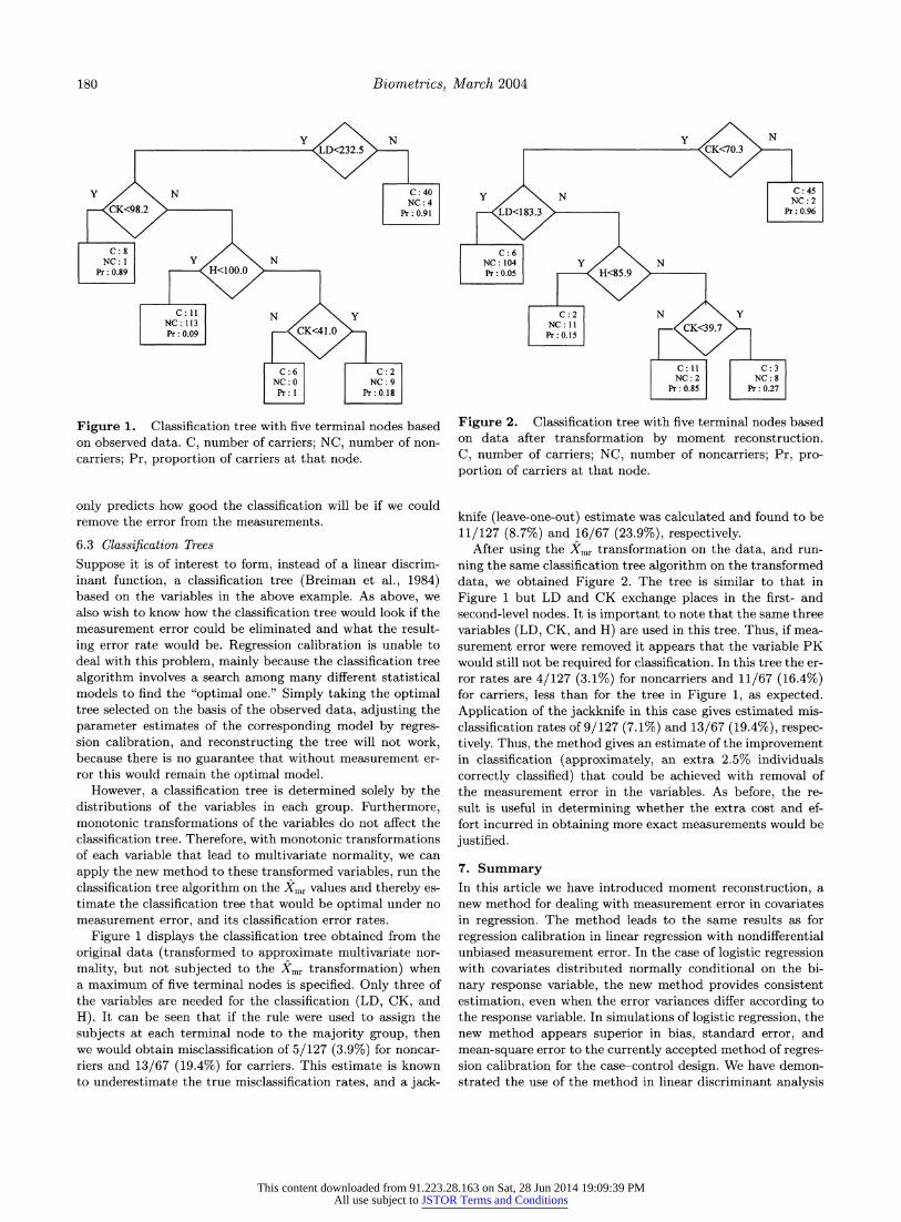
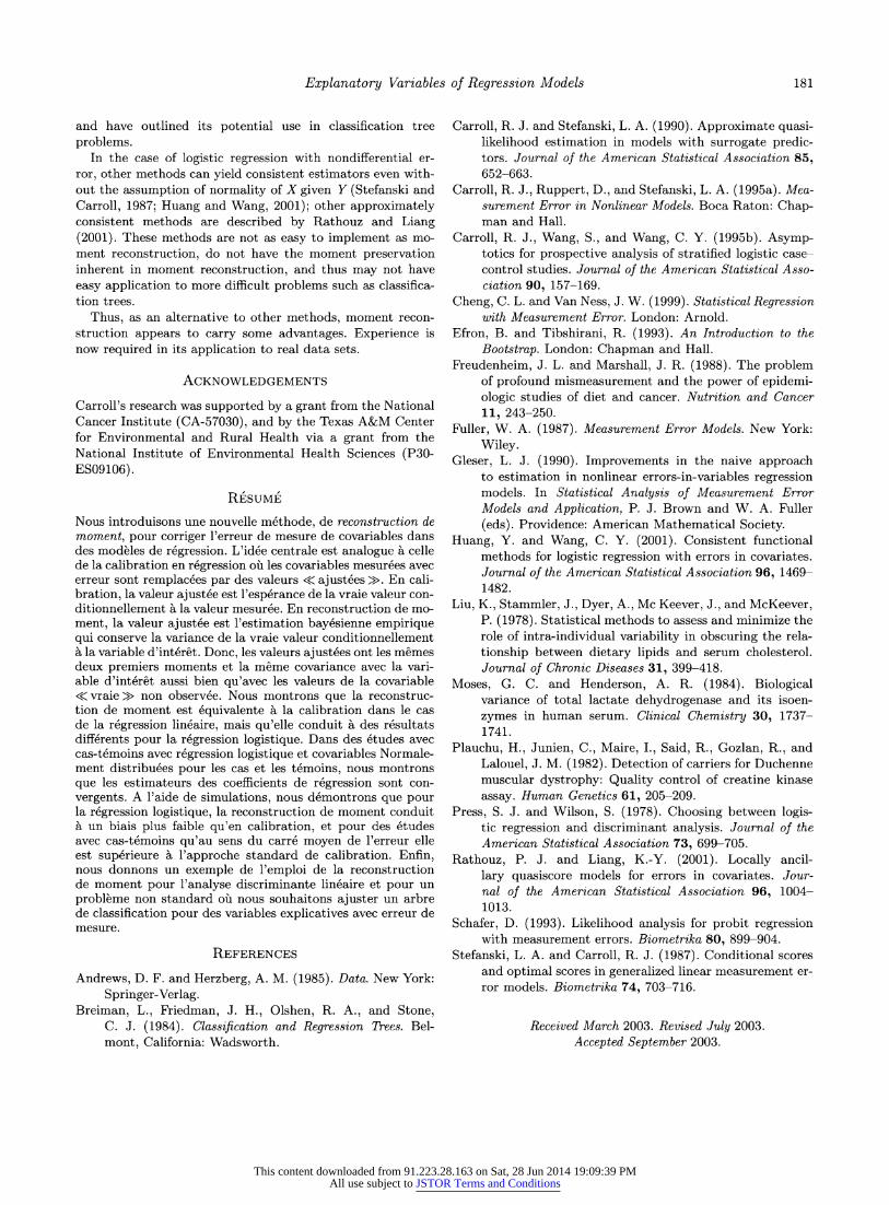
Figure 1. Classification tree with five terminal nodes based on observed data. C, number of carriers; NC, number of noncarriers; Pr, proportion of carriers at that node.

only predicts how good the classification will be if we could remove the error from the measurements.

6.3 Classification Trees

Suppose it is of interest to form, instead of a linear discriminant function, a classification tree (Breiman et al., 1984) based on the variables in the above example. As above, we also wish to know how the classification tree would look if the measurement error could be eliminated and what the resulting error rate would be. Regression calibration is unable to deal with this problem, mainly because the classification tree algorithm involves a search among many different statistical models to find the "optimal one." Simply taking the optimal tree selected on the basis of the observed data, adjusting the parameter estimates of the corresponding model by regression calibration, and reconstructing the tree will not work, because there is no guarantee that without measurement error this would remain the optimal model.

However, a classification tree is determined solely by the distributions of the variables in each group. Furthermore, monotonic transformations of the variables do not affect the classification tree. Therefore, with monotonic transformations of each variable that lead to multivariate normality, we can apply the new method to these transformed variables, run the classification tree algorithm on the Xmr values and thereby estimate the classification tree that would be optimal under no measurement error, and its classification error rates.

Figure 1 displays the classification tree obtained from the original data (transformed to approximate multivariate normality, but not subjected to the Xmr transformation) when a maximum of five terminal nodes is specified. Only three of the variables are needed for the classification (LD, CK, and H). It can be seen that if the rule were used to assign the subjects at each terminal node to the majority group, then we would obtain misclassification of 5/127 (3.9%) for noncarriers and 13/67 (19.4%) for carriers. This estimate is known to underestimate the true misclassification rates, and a jack-

Y N CK<70.3

C: 45

NC:2 LD<183.3 Pr :0.96

C:6

NC : 104 Y N Pr : 0.05 - i H<85.9

C:2 N Y NC: 11

CK<39.7 P r : 0 .15

C:11 C:3 NC: 2 NC: 8

Pr : 0.85 Pr : 0.27

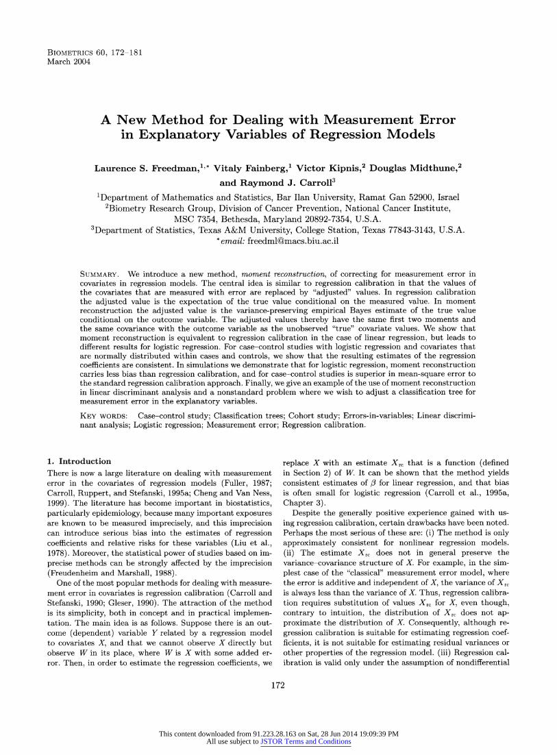
Figure 2. Classification tree with five terminal nodes based on data after transformation by moment reconstruction. C, number of carriers; NC, number of noncarriers; Pr, proportion of carriers at that node.

knife (leave-one-out) estimate was calculated and found to be

11/127 (8.7%) and 16/67 (23.9%), respectively. After using the Xmr transformation on the data, and run-

ning the same classification tree algorithm on the transformed data, we obtained Figure 2. The tree is similar to that in Figure 1 but LD and CK exchange places in the first- and second-level nodes. It is important to note that the same three variables (LD, CK, and H) are used in this tree. Thus, if measurement error were removed it appears that the variable PK would still not be required for classification. In this tree the error rates are 4/127 (3.1%) for noncarriers and 11/67 (16.4%) for carriers, less than for the tree in Figure 1, as expected. Application of the jackknife in this case gives estimated misclassification rates of 9/127 (7.1%) and 13/67 (19.4%), respectively. Thus, the method gives an estimate of the improvement in classification (approximately, an extra 2.5% individuals correctly classified) that could be achieved with removal of the measurement error in the variables. As before, the result is useful in determining whether the extra cost and ef- fort incurred in obtaining more exact measurements would be justified.

7. Summary In this article we have introduced moment reconstruction, a new method for dealing with measurement error in covariates in regression. The method leads to the same results as for regression calibration in linear regression with nondifferential unbiased measurement error. In the case of logistic regression with covariates distributed normally conditional on the binary response variable, the new method provides consistent estimation, even when the error variances differ according to the response variable. In simulations of logistic regression, the new method appears superior in bias, standard error, and mean-square error to the currently accepted method of regression calibration for the case-control design. We have demon- strated the use of the method in linear discriminant analysis




and have outlined its potential use in classification tree problems.

In the case of logistic regression with nondifferential error, other methods can yield consistent estimators even without the assumption of normality of X given Y (Stefanski and Carroll, 1987; Huang and Wang, 2001); other approximately consistent methods are described by Rathouz and Liang (2001). These methods are not as easy to implement as moment reconstruction, do not have the moment preservation inherent in moment reconstruction, and thus may not have easy application to more difficult problems such as classification trees.

Thus, as an alternative to other methods, moment reconstruction appears to carry some advantages. Experience is now required in its application to real data sets.

ACKNOWLEDGEMENTS

Carroll's research was supported by a grant from the National Cancer Institute (CA-57030), and by the Texas A&M Center for Environmental and Rural Health via a grant from the National Institute of Environmental Health Sciences (P30- ES09106).

RESUM?E

Nous introduisons une nouvelle methode, de reconstruction de moment, pour corriger l'erreur de mesure de covariables dans des modules de regression. L'id~e centrale est analogue a celle de la calibration en regression ofi les covariables mesur6es avec erreur sont remplacees par des valeurs < ajustees >. En calibration, la valeur ajustie est l'esperance de la vraie valeur conditionnellement a la valeur mesuree. En reconstruction de moment, la valeur ajustee est l'estimation bayesienne empirique qui conserve la variance de la vraie valeur conditionnellement a la variable d'interit. Donc, les valeurs ajusties ont les memes deux premiers moments et la meme covariance avec la variable d'interit aussi bien qu'avec les valeurs de la covariable <vraie > non observ&e. Nous montrons que la reconstruction de moment est equivalente a la calibration dans le cas de la rigression lineaire, mais qu'elle conduit a des resultats diffrents pour la r6gression logistique. Dans des etudes avec cas-timoins avec regression logistique et covariables Normale- ment distributes pour les cas et les tPmoins, nous montrons que les estimateurs des coefficients de rPgression sont con- vergents. A l'aide de simulations, nous dimontrons que pour la rPgression logistique, la reconstruction de moment conduit a un biais plus faible qu'en calibration, et pour des etudes avec cas-tPmoins qu'au sens du carre moyen de l'erreur elle est superieure a l'approche standard de calibration. Enfin, nous donnons un exemple de l'emploi de la reconstruction de moment pour l'analyse discriminante liniaire et pour un problkme non standard oi nous souhaitons ajuster un arbre de classification pour des variables explicatives avec erreur de mesure.

REFERENCES

Andrews, D. F. and Herzberg, A. M. (1985). Data. New York: Springer-Verlag.

Breiman, L., Friedman, J. H., Olshen, R. A., and Stone, C. J. (1984). Classification and Regression Trees. Bel- mont, California: Wadsworth.

Carroll, R. J. and Stefanski, L. A. (1990). Approximate quasi- likelihood estimation in models with surrogate predic- tors. Journal of the American Statistical Association 85, 652-663.

Carroll, R. J., Ruppert, D., and Stefanski, L. A. (1995a). Mea- surement Error in Nonlinear Models. Boca Raton: Chap- man and Hall.

Carroll, R. J., Wang, S., and Wang, C. Y. (1995b). Asymp- totics for prospective analysis of stratified logistic case- control studies. Journal of the American Statistical Asso- ciation 90, 157-169.

Cheng, C. L. and Van Ness, J. W. (1999). Statistical Regression with Measurement Error. London: Arnold.

Efron, B. and Tibshirani, R. (1993). An Introduction to the Bootstrap. London: Chapman and Hall.

Freudenheim, J. L. and Marshall, J. R. (1988). The problem of profound mismeasurement and the power of epidemi- ologic studies of diet and cancer. Nutrition and Cancer 11, 243-250.

Fuller, W. A. (1987). Measurement Error Models. New York: Wiley.

Gleser, L. J. (1990). Improvements in the naive approach to estimation in nonlinear errors-in-variables regression models. In Statistical Analysis of Measurement Error Models and Application, P. J. Brown and W. A. Fuller

(eds). Providence: American Mathematical Society. Huang, Y. and Wang, C. Y. (2001). Consistent functional

methods for logistic regression with errors in covariates. Journal of the American Statistical Association 96, 1469- 1482.

Liu, K., Stammler, J., Dyer, A., Mc Keever, J., and McKeever, P. (1978). Statistical methods to assess and minimize the role of intra-individual variability in obscuring the rela- tionship between dietary lipids and serum cholesterol. Journal of Chronic Diseases 31, 399-418.

Moses, G. C. and Henderson, A. R. (1984). Biological variance of total lactate dehydrogenase and its isoen- zymes in human serum. Clinical Chemistry 30, 1737- 1741.

Plauchu, H., Junien, C., Maire, I., Said, R., Gozlan, R., and Lalouel, J. M. (1982). Detection of carriers for Duchenne muscular dystrophy: Quality control of creatine kinase assay. Human Genetics 61, 205-209.

Press, S. J. and Wilson, S. (1978). Choosing between logistic regression and discriminant analysis. Journal of the American Statistical Association 73, 699-705.

Rathouz, P. J. and Liang, K.-Y. (2001). Locally ancil- lary quasiscore models for errors in covariates. Jour- nal of the American Statistical Association 96, 1004- 1013.

Schafer, D. (1993). Likelihood analysis for probit regression with measurement errors. Biometrika 80, 899-904.

Stefanski, L. A. and Carroll, R. J. (1987). Conditional scores and optimal scores in generalized linear measurement error models. Biometrika 74, 703-716.

Received March 2003. Revised July 2003. Accepted September 2003.



Documents

A New Method for Dealing with Measurement Error in Explanatory Variables of Regression Models