A NEW METHOD FOR ANALYSING AND … · RESUMEN: Los resultados de las investigaciones sobre la respuesta térmica del ... Mazhitova et al. 2004; Lewkowicz, 2007; Ramos et al., 2008;

DOI: http://doi.org/10.18172/cig.3373 © Universidad de La Rioja

Cuadernos de Investigación GeográficaGeographical Research Letters

2018 Nº 44 (1) pp. 293-320ISSN 0211-6820

eISSN 1697-9540

293Cuadernos de Investigación Geográfica 44 (1), 2018, pp. 293-320

A NEW METHOD FOR ANALYSING AND REPRESENTING GROUND TEMPERATURE VARIATIONS IN COLD

ENVIRONMENTS. THE FUEGIAN ANDES, TIERRA DEL FUEGO, ARGENTINA

M. OLIVEIRA1, A. PÉREZ-ALBERTI2*, R.M. CRUJEIRAS1, A. RODRÍGUEZ-CASAL1, F. CASTILLO-RODRÍGUEZ3

1Departamento de Estatística, Análise Matemática e Optimización, Universidade de Santiago de Compostela, Spain.

2Departamento de Xeografía, Universidade de Santiago de Compostela, Spain. 3Consellería de Educación. Xunta de Galicia, Santiago de Compostela, Spain.

ABSTRACT: The thermal response of soils in cold environments has been investigated in numerous studies. The data considered here were obtained in a study carried out in Tierra del Fuego, Argentina, as part of the IV International Polar Year. Temperature sensors were installed at ground level (0) and depths of -10, -20 and -60 cm in the study area, with the aim of characterizing the thermal response by detecting diurnal and annual variations.

The study has two main aims. The first is to present and discuss the study findings regarding the thermal response of a soil in a sub-Antarctic environment by using classical descriptive analysis. The second, closely related, aim is to apply some novel statistical tools that would help improve this description. The study of freeze-thaw patterns can be approached from a non-parametric perspective, while taking into account the cyclical nature of the data. Data are considered cyclical when they can be represented on a unit circle, as with the hours in which certain events occur throughout a day (e.g. freezing and thawing). Analysis of this type of data is very different from the analysis of scalar data, as regards both descriptive and graphical measures. The application in this study of methods used to represent and analyse cyclical data improved visualization of the data and interpretation of the analytical findings. The main contribution of the present study is the use of estimators of the nuclear type density and derived techniques, such as the CircSiZer map, which enabled identification of significant freeze-thaw patterns. In addition, the relationships between the temperature recordings at different points were analysed using Taylor diagrams.

Oliveira et al.

294 Cuadernos de Investigación Geográfica 44 (1), 2018, pp. 293-320

Un nuevo método para analizar y representar las variaciones de temperatura del suelo en ambientes fríos. Los Andes Fueguinos, Tierra del Fuego, Argentina

RESUMEN: Los resultados de las investigaciones sobre la respuesta térmica del suelo en ambientes fríos han sido recogidos en un gran número de artículos. Las muestras de datos consideradas en este trabajo pertenecen también a un ambiente frío y se han obtenido de una investigación realizada en Tierra del Fuego, Argentina, bajo los auspicios del Año Polar Internacional. Con el fin de caracterizar la respuesta térmica, se instalaron diferentes sensores de temperatura a 0, -10, -20 y -60 cm de profundidad, permitiendo la detección de variaciones anuales y diarias.

Este trabajo persigue un doble objetivo. Por un lado, la presentación de resultados y discusión sobre los mismos en relación al comportamiento térmico del suelo en un ambiente subantártico. Por otro lado, y apoyando al objetivo anterior, se introducen algunas herramientas estadísticas novedosas en este contexto, si bien el estudio se acompaña de análisis descriptivos clásicos. El estudio de patrones de congelación y descongelación puede enfocarse desde una perspectiva no paramétrica, a la vez que se tiene en cuenta la naturaleza circular (cíclica) de los datos. Una muestra de datos se considera circular cuando puede representarse sobre un círculo de radio unidad. Esto ocurre, por ejemplo, con las horas en las que suceden determinados eventos a lo largo de un día (por ejemplo, congelaciones y descongelaciones). El análisis de este tipo de datos es radicalmente distinto del que se realiza sobre datos escalares, tanto en lo que se refiere a medidas descriptivas como a métodos gráficos. El uso de representacio-nes y herramientas propias del análisis de datos circulares realizado en este trabajo permite una mejor visualización de los datos y de los resultados de su análisis. Como principal aportación, cabe destacar el uso de estimadores de la densidad tipo núcleo y técnicas derivadas, como el mapa CircSiZer, que identifica patrones significativos de congelación/descongelación. Además, el análisis de las relaciones entre registros de temperaturas en distintos puntos se presenta a través del uso de Diagramas de Taylor.

Key words: active layer, temperature sensors, non-parametric methods, circular data, Taylor diagram, Tierra del Fuego (Argentina).

Palabras clave: capa activa, sensores de temperatura, métodos no paramétricos, datos circulares, diagrama de Taylor, Tierra del Fuego (Argentina).

Received: 14 July 2017 Accepted: 14 September 2017

Corresponding author: Augusto Pérez-Alberti, Departamento de Xeografía, Universidad de Santiago de Compostela, Praza da Universidad 1, 15783 Santiago de Compostela, Spain. E-Mail address: [email protected]

1. Introduction

Study of the thermal response of soil is very important for understanding the functioning of the dynamics of the slopes. Frozen ground is widespread in the mountainous

Analysing and representing ground temperature variations in cold environments


areas of the Subantarctic region, such as Tierra del Fuego (Argentina), and geomorphic processes have a significant influence on landscape evolution (Kneisel et al., 2008). The soil temperature regime strongly influences geomorphological, hydrological and related phenomena, such as frost creep processes, needle-ice creep, shallow solifluction, upfreezing of granules (Washburn, 1979; Williams and Smith, 1989), patterned ground, solifluction sheets (cf. Matsuoka, 2001) and terracettes, all of which are manifested in the active layer (Leszkiewicz and Caputa, 2004). Other types of microforms, often of transient character, are associated with the action of needle-ice and include needle-ice raked ground, gaps around stones, nubbins and fine-earth flags (Washburn, 1979).

The upper level of a soil undergoing freeze-thaw processes is called the active layer, which has been defined as “the layer of ground above permafrost which thaws in summer and freezes again in winter” (Muller, 1947). As the same author also defined frozen ground as “ground that has a temperature of 0ºC or lower” (Muller, 1947), the definition of the active layer can, unequivocally, be interpreted in terms of temperature. The term has been widely adopted in the English language definitions of permafrost terms (e.g. Brown and Kupsch, 1974), in books on permafrost (e.g. Washburn, 1979; Johnston, 1981; Harris et al., 1988, Andersland and Ladanyi, 1994), and in other articles (e.g. Parmuzina, 1978; Mackay, 1983). The depth of thaw penetration, or the active-layer thickness (ALT), in permafrost-affected soils mainly depends on the intensity and duration of the cold, snow cover, vegetation, soil texture, rock type, permafrost continuity, precipitation and cloud cover (Goodrich, 1982; French, 2013; Guglielmin et al., 2003).

Numerous studies of the dynamics of the active layer have been conducted over many years (Chambers, 1966a, 1966b, 1967, 1970; Shiklomanov et al., 1989; Brown et al., 2000; Mazhitova et al. 2004; Lewkowicz, 2007; Ramos et al., 2008; Guglielmin, 2006: Streletskiy et al. 2008; Adlam et al., 2010; Vieira et al., 2010; Zao et al., 2010. Most of these studies include profiles that represent the temperature distribution at depth (e.g. Romanovsky et al., 2010 [Figure 4, page 112]; Solomon et al., 2008 [Figures 2 and 3, page 1677]) but not the daily freeze-thaw cycles.

The aim of this study is twofold. On the one hand, it focuses on analysing the variability in the ground thermal regime in the mountains of Tierra del Fuego, both in seasonal and daily patterns. On the other hand, some novel exploratory graphical and numerical tools were used to better explain the aforementioned variability in temperature regimes and to better understand the daily patterns of freeze-thaw cycles. Some details on data recording and statistical methods (mainly nonparametric) are provided.

1.2. Study area

Data were collected on the Isla Grande of Tierra del Fuego (Fig. 1), located between 52º and 56º South latitude and 63º and 75º West longitude, within an area of 20,180 km2. The existence of permafrost in the Fuegian Andes, at altitudes exceeding 1000 m, was unknown until recently (Valcárcel et al., 2008) and indicates evident cryonival activity (Valcárcel et al., 2006). However, the degree of mobility of the soil surface layer has not yet been determined.

Oliveira et al.


Figure 1. Location of the study area and measurement stations.

Tierra de Fuego is relatively close to the great ice sheet of the Antarctic continent, which places the Fuegian archipelago between the southern flanks of the Pacific and Atlantic cells of subtropical high pressures and the low subpolar pressures that scarcely vary in intensity or location throughout the year. The persistence of the leading centres in the region’s pressure field guarantees the prevalence of the west flows in the whole territory throughout the year (Walter and Box, 1983; Burgos, 1985; Tuhkanen, 1992; Iturraspe and Urciuolo, 2000). This proximity favours more intense cyclogenesis and rapid transition of the depressions associated with the zonal flows of the west and southwest components. These flows dominate the atmospheric scene throughout the year at these latitudes and give rise to a high degree of instability. Such instability is caused when the flows reach the Fuegian coasts dragged by winds from the third and fourth quadrants, with an annual appearance higher than the 75%.

The zonal orientation of the Andean mountain range is not an optimal arrangement for intercepting or mitigating the humidity associated with the frontal systems. The complex topography provides effective orographic control in the spatial distribution of precipitation at meso and micro scales (Schroeder et al., 1989) and, above all, marked thermo-pluviometric gradients reflected in altitudinal vegetation sequences, in which the limits of survival of the species are evident.

The scarcity and discontinuity of the meteorological data have led some authors to estimate altitudinal temperature gradients in the free atmosphere and to use this data



as an accurate estimation of the slope of the gradient. The annual variation in the mean temperature is expressed by the equation y= -0.0056193x +5.74 (Puigdefábregas et al., 1988). This variation implies estimated thermal gradients between 0.43-0.7ºC each 100 m in July and December, respectively. The annual average is 0.55ºC/100 m (Iturraspe et al., 1989). These gradient values guarantee low temperature records below zero in winter at summits, taking into account that the annual average temperature at Ushuaia station –sea level– is 5.9ºC (data provided by the Statistical Service of the Argentinian SMN). The mean altitudinal precipitation gradient has been estimated to be 120 mm / 100 m (Barrera et al., 2000).

Seasonal rainfall is low, with contributions in all months of the year, although with modest volumes, slightly above 500 mm (valid data from the stations in the Beagle channel). Some 35% of the annual volume of precipitation recorded occurs in the form of snow, with a higher frequency between June and September. The annual wind regime reaches maximal intensity in spring and summer. In this period, the annual average speed is higher than 12 ms-1 and the maximum exceeds 30 ms-1. The winds with a southwest component are especially remarkable in spring and summer, and in the latter are responsible for a significant reduction in the maximum temperature and therefore in the annual thermal oscillation. They also cause a high level of evapotranspiration. This cool, windy, scarcely-marked summer is one of the most characteristic features of the Fuegian climate (Allué et al., 2010). Dynamic phenomena caused by the relief forms include the drainage of cold flows –catabolic winds– which occur in the summit areas of the heart of the large island of Tierra del Fuego.

The daily amplitude in the winter season is generally attenuated, especially in situations that trigger episodes of precipitation, both in the form of snow and liquid. In these episodes, linked to the transition of fronts associated with oceanic disturbances, the temperature regime is controlled by the thermal nature of the mass associated with the frontal discontinuities rather than by the insolation. The fact that the thermometry is characterized by a contained thermal amplitude, relative to the location latitude, is reinforced by the surrounding oceanic mass. This phenomenon becomes more evident in the winter months. In the summit zones, the thermal regime of the active layer reflects seasonal and interannual climatic variability, as its drift is a direct function of the energy exchange with the atmospheric surface layer (Ramos et al., 2002).

3. Data and methods

3.1. Data recording

Four measuring stations were installed at different altitudes (between 750 m and 1100 m) of the Alvear Glaciar (Figure 1) to record soil temperature data. Two of the stations were placed in a flat sector at an altitude of 1100 m (one in an area dominated by schist rocks and phorphyries): Station 1 (Calm) and Station 2 (Circle). A third station was placed on the hillside of the Tristén valley, at an altitude of 989 m (Station 3, Tristen) and the fourth was located in the surroundings of the Alvear lake, at an altitude of 750 m (Station 4, Alvear Lake). In all sites, U12 Hobo dataloggers were placed at depths of 0, -10, -20 and

Oliveira et al.


-60 cm below the ground. For each station and depth, temperature was recorded hourly between February 2008 and January 2009, providing a dataset of 8712 observations in each case. During the same period, the air temperature was recorded at a height of 80 cm in a fifth site (Tower).

3.2. Statistical methods

The data obtained were examined using different statistical tests. First, as the temperatures were recorded at various depths at each station, descriptive analysis at each depth may help to provide a rough picture of the data. Numerical and graphical analyses can be performed for this purpose. Hence, the basic information contained in summary statistics, such as mean, standard deviation, median and quartiles, can be completed with some insight into the data distribution. Violin plots (Hintze and Nelson, 1998) will be specifically considered for this purpose. A violin plot is essentially the combination of a boxplot with a smooth (kernel) density estimator. For a given data sample, a boxplot is obtained by considering the quartiles for constructing a central box (limits Q1 and Q3, and an inside horizontal line for the median value) and the upper and lower limits obtained by comparing the Q3+1.5IQR and Q1-1.5IQR values with the largest and smallest sample values, where IQR=Q3-Q1 is the interquartile range). Asymmetric patterns or outliers can be easily detected by examining boxplots. However, boxplots do not reflect multimodality, in the sense of having more than one group of data in the underlying distribution.

A kernel density estimator (Silverman, 1998) is a smooth estimator of the probability density function for a given dataset, which can be viewed as a continuous (and smooth) version of a mobile histogram. Technically, given a series of data x1,x2,…,xn corresponding to a variable X with (unknown) density f, the kernel density estimator is defined as follows:

𝑓𝑓"(𝑥𝑥) =1𝑛𝑛 𝐾𝐾"(𝑥𝑥 − 𝑥𝑥+)

,

+-.

,

which can be interpreted, for a fixed x, as an average of some weights depending on the distances between x and the data sample values, xi with i=1,…,n. The weights are determined by Kh(·), a rescaled kernel, which places greater weight on the data observations closer to x. A suitable value of the h parameter, called the bandwidth, must be selected. Many methods of bandwidth selection are available in the statistical literature (see Silverman, 1998 for some examples). In the present study, kernel density estimates were computed using Silverman’s rule-of-thumb to select the bandwidth. For large sample sizes, binning is employed. This estimator produces a smooth curve, which can be plotted by itself or by attaching it (symmetrically) to a boxplot, providing a violin plot.

As already mentioned, the statistical analysis performed was not only restricted to temperature values and the daily freeze thaw cycles were also considered of interest. A cycle is the period of time during which the temperature is always greater or lower than 0ºC. For this purpose (identifying daily patterns of thawing and freezes), cycle changes



(temperatures varying from negative to positive or vice versa) can be viewed as points in a circle throughout the day and hence can be treated as cyclical data. Apart from counting the number of such occurrences, which is interesting for comparison at different depths, further analysis of cyclical data can be performed. Specifically, the kernel density estimator introduced above can be adapted to a cyclical setting (see e.g. Oliveira et al., 2012), considering a suitable kernel function accounting for the periodic nature of the data. The estimator will also depend on the smoothing parameter (bandwidth) selected, and different values of this quantity will therefore provide smooth or rough estimators.

A central question in the analysis of cyclical data is the identification of which features are (statistically) significant, rather than being sampling artefacts, e.g. whether cycle changes are uniformly distributed throughout the day or at a specific time. The Significant Zero crossings of the derivative (SiZer) method of Chaudhuri and Marron (1999) can be used to detect such significance. SiZer is based on two notions: the first is the notion of scale space whereby instead of trying to find a bandwidth that provides the closest match to the unknown true density, we examine the whole range of bandwidths and explore the different features that occur on different scales. Secondly, peaks and troughs are identified by finding the regions of significant gradient (zero crossings of the derivative), i.e. the significance of peaks and valleys in a family of smooth estimators is based on confidence intervals for the derivative 𝑓𝑓"#(𝑥𝑥)

𝑓𝑓"(𝑥𝑥)

in scale space. The information provided by the confidence intervals is visually represented by the SiZer map. In the SiZer colour map, blue regions indicate locations of x and h where 𝑓𝑓"#(𝑥𝑥)

𝑓𝑓"(𝑥𝑥)

is significantly positive (

𝑓𝑓"#(𝑥𝑥) 𝑓𝑓"(𝑥𝑥)

is significantly increasing), red indicates locations where 𝑓𝑓"#(𝑥𝑥) 𝑓𝑓"(𝑥𝑥)

is significantly negative, (

𝑓𝑓"#(𝑥𝑥) 𝑓𝑓"(𝑥𝑥)

is significantly decreasing), and purple indicates where 𝑓𝑓"#(𝑥𝑥)

𝑓𝑓"(𝑥𝑥)

is not significantly different from zero. Regions in which there are not enough data to make statements about significance are coloured grey. Thus, at a given bandwidth, h, a significant peak can be identified when a region of significant positive gradient is followed by a region of significant negative gradient (i.e. blue-red pattern), and a significant trough by the opposite (red-blue pattern).

Again considering the analysis of cyclical data (cycle changes), the illustration of increasing and decreasing patterns in a density for a family of smooth estimators enables identification of persistent features at different scales of detail. This illustration is called a CircSizer map (Oliveira et al., 2014), which is an extension of the SiZer map. More details about its construction will be given below, in relation to the analysis of the statistical findings.

The previous techniques (numerical summaries, violin plots and CircSizers for cyclical data) provide a marginal view of the temperature series accounting for different patterns. This marginal view does not intend to illustrate the relation between records at different sites or, more interestingly, at the same site but at different heights, for instance, between ground and air temperature. We can consider two data samples, denoted by x1,x2,…,xn and y1,y2,…, yn (ground and air temperature, respectively, at n time moments). The relation between both variables can be illustrated using a Taylor diagram (Taylor, 2001), a two dimensional plot which provides a concise statistical summary of how well

Oliveira et al.


patterns match each other in terms of their correlation, the root mean square (RMS) difference and the ratio of their variances.

To construct a Taylor diagram, we first consider the (Pearson) correlation coefficient between the two variables:

𝑅𝑅 =1𝑛𝑛 𝑥𝑥& − 𝑥𝑥 𝑦𝑦& − 𝑦𝑦)

&*+

𝑆𝑆-𝑆𝑆.

where 𝑅𝑅 =

1𝑛𝑛 𝑥𝑥& − 𝑥𝑥 𝑦𝑦& − 𝑦𝑦)

&*+

𝑆𝑆-𝑆𝑆. and

𝑅𝑅 =1𝑛𝑛 𝑥𝑥& − 𝑥𝑥 𝑦𝑦& − 𝑦𝑦)

&*+

𝑆𝑆-𝑆𝑆.

, 𝑅𝑅 =1𝑛𝑛 𝑥𝑥& − 𝑥𝑥 𝑦𝑦& − 𝑦𝑦)

&*+

𝑆𝑆-𝑆𝑆. and 𝑅𝑅 =

1𝑛𝑛 𝑥𝑥& − 𝑥𝑥 𝑦𝑦& − 𝑦𝑦)

&*+

𝑆𝑆-𝑆𝑆. represent the mean and standard deviations of the observed

samples. The correlation coefficient takes values between -1 and 1, with the extremes indicating a perfect (negative or positive) linear correlation.

Differences between the two samples can be measured with the RMS difference E, given by the following:

𝐸𝐸 =1𝑛𝑛 𝑥𝑥& − 𝑥𝑥 𝑦𝑦& − 𝑦𝑦 *

+

&,!

.*

for the definitions of R and E, it is easy to see that

𝐸𝐸" = 𝑆𝑆%" + 𝑆𝑆'" − 2𝑆𝑆%𝑆𝑆'𝑅𝑅,

and taking into account the law of the cosines, it is possible to construct a diagram that quantifies the degree of similarity between the two samples. Generally, one of the samples will be called the “reference”, and the other one will be referred as the “test” sample, and the aim of Taylor diagrams is to quantify how close both samples are, in terms of correlation and also accounting for the standard deviations in both samples. In these graphs, the radial distances from the origin to the points are proportional to the standard deviations of the pattern, and the azimuthal positions give the correlation coefficient between the two fields. The radial lines are labelled by the cosine of the angle with the abscissa. The dashed lines measure the distance from the reference point and indicate the RMS error (once any overall bias has been removed). The point representing the reference field is plotted along the abscissa.

All the data analysis and figures were produced using R software, an open source programming language and environment for statistical computing and graphics (R Core Team, 2016).

4. Results

As already mentioned, four temperature measurement stations were installed at ground level and at depths of -10, -20 and -60 cm in four sites that differ in relation to location and sediment cover. Air temperature was recorded at a fifth measurement station (Tower) (at +80 cm). The main aim of the recording was to determine any differences in temperature and the effect of the air temperature on the ground temperature at the four sites.



4.1. Descriptive analysis

Tables 1-4 show some summary statistics for the temperature series at the different depths in Stations 1, 2, 3 and 4 respectively. Table 5 shows some results for the air temperature in the Tower. All of the figures indicate that the temperature is more variable during the first and last months of the year, coinciding with the summer season. This was particularly noticeable at the ground level and at -10 cm, whilst at -20 and -60 cm the differences in temperature throughout the year were smaller. The figures also indicate that the temperature was less variable at greater depth. In other words, the temperature at the lower levels of soil was more stable than that at the surface. The effect of the air temperature on the ground temperature decreased with increasing depth.

Table 1. Descriptive statistics for temperature data in Station 1. Mean (and standard deviation), minimum, maximum and quartiles.

Station 1 Min. 1stQu. Median Mean (Std. dev) 3rdQu. Max.

0 cm -7.58 -1.81 -0.20 0.62 (3.74) 1.27 19.32

-10 cm -6.20 -1.93 -0.40 0.43 (3.21) 1.97 13.98

-20 cm -3.81 -1.78 -0.40 0.40 (2.69) 2.40 8.96

-60 cm -2.54 -1.50 -0.40 0.36 (2.17) 2.15 6.03


Station 2 Min. 1stQu. Median Mean (Std. dev) 3rdQu. Max.0 cm -9.51 -4.17 -0.48 -0.44 (4.79) 1.86 20.75

-10 cm -8.30 -3.93 -0.40 -0.52 (4.02) 2.21 12.80-20 cm -7.45 -3.69 -0.28 -0.54 (3.48) 2.13 8.52-60 cm -6.58 -3.51 -0.26 -0.66 (2.98) 1.62 6.10


Station 3 Min. 1stQu. Median Mean (Std. dev.) 3rdQu. Max.0 cm -11.18 -2.28 -0.17 0.36 (4.61) 1.29 26.48

-10 cm -8.07 -1.93 0.05 0.48 (3.42) 2.56 15.22-20 cm -6.33 -1.87 -0.06 0.25 (2.74) 2.29 8.62-60 cm -3.51 -1.13 0.22 0.51 (1.92) 1.72 6.03

Oliveira et al.



Station 4 Min. 1stQu. Median Mean (Std. dev) 3rdQu. Max.0 cm -10.86 -2.22 -0.31 1.23 (5.83) 3.70 38.62

-10 cm -7.19 -1.33 0.05 1.10 (3.42) 3.49 14.03-20 cm -7.15 -1.76 -0.37 0.62 (3.31) 2.90 11.13-60 cm -6.01 -1.33 -0.06 0.98 (3.12) 3.25 9.68

Table 5. Descriptive statistics for temperature data in Tower. Mean (and standard deviation), minimum, maximum and quartiles.

Tower Min. 1stQu. Median Mean (Std. dev) 3rdQu. Max.80 cm -11.92 -4.27 -1.34 -0.33 (5.37) 2.94 22.62

Temperature variations followed the same trend at all four levels and at the four locations. The temperature sometimes remained constant (about 0ºC) during October-November; however, this was due to an error in the measurement station caused by the low temperatures. For this reason and as there are clearly not four seasons in view of temperature series, we analysed the temperatures in two-month periods.

Figure 2. Violin plots for all the stations, at different depths. From left to right and from top to bottom: Station 1, Station 2, Station 3 and Station 4. Black: boxplot elements. Grey: area under

the kernel density estimator, symmetrized around the boxplot.



Figure 3. Violin plots for Station 1 for two-month periods. From left to right and from top to bottom: December-January, February-March, April-May, June- July, August-September and October-November. In each plot, representations at different depths. Black: boxplot elements.

Grey: area under the kernel density estimator, symmetrized around the boxplot.

Oliveira et al.








Oliveira et al.




Figure 7. Violin plots for Tower. Left: global. Right: two-month periods. Black: boxplot elements. Grey: area under the kernel density estimator, symmetrized around the boxplot.



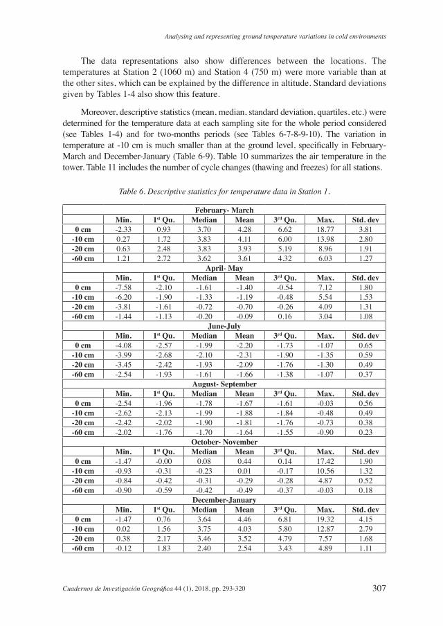
The data representations also show differences between the locations. The temperatures at Station 2 (1060 m) and Station 4 (750 m) were more variable than at the other sites, which can be explained by the difference in altitude. Standard deviations given by Tables 1-4 also show this feature.

Moreover, descriptive statistics (mean, median, standard deviation, quartiles, etc.) were determined for the temperature data at each sampling site for the whole period considered (see Tables 1-4) and for two-months periods (see Tables 6-7-8-9-10). The variation in temperature at -10 cm is much smaller than at the ground level, specifically in February-March and December-January (Table 6-9). Table 10 summarizes the air temperature in the tower. Table 11 includes the number of cycle changes (thawing and freezes) for all stations.

Table 6. Descriptive statistics for temperature data in Station 1.

February- MarchMin. 1st Qu. Median Mean 3rd Qu. Max. Std. dev

0 cm -2.33 0.93 3.70 4.28 6.62 18.77 3.81-10 cm 0.27 1.72 3.83 4.11 6.00 13.98 2.80-20 cm 0.63 2.48 3.83 3.93 5.19 8.96 1.91-60 cm 1.21 2.72 3.62 3.61 4.32 6.03 1.27

April- MayMin. 1st Qu. Median Mean 3rd Qu. Max. Std. dev

0 cm -7.58 -2.10 -1.61 -1.40 -0.54 7.12 1.80-10 cm -6.20 -1.90 -1.33 -1.19 -0.48 5.54 1.53-20 cm -3.81 -1.61 -0.72 -0.70 -0.26 4.09 1.31-60 cm -1.44 -1.13 -0.20 -0.09 0.16 3.04 1.08

June-JulyMin. 1st Qu. Median Mean 3rd Qu. Max. Std. dev

0 cm -4.08 -2.57 -1.99 -2.20 -1.73 -1.07 0.65-10 cm -3.99 -2.68 -2.10 -2.31 -1.90 -1.35 0.59-20 cm -3.45 -2.42 -1.93 -2.09 -1.76 -1.30 0.49-60 cm -2.54 -1.93 -1.61 -1.66 -1.38 -1.07 0.37

August- SeptemberMin. 1st Qu. Median Mean 3rd Qu. Max. Std. dev

0 cm -2.54 -1.96 -1.78 -1.67 -1.61 -0.03 0.56-10 cm -2.62 -2.13 -1.99 -1.88 -1.84 -0.48 0.49-20 cm -2.42 -2.02 -1.90 -1.81 -1.76 -0.73 0.38-60 cm -2.02 -1.76 -1.70 -1.64 -1.55 -0.90 0.23

October- NovemberMin. 1st Qu. Median Mean 3rd Qu. Max. Std. dev

0 cm -1.47 -0.00 0.08 0.44 0.14 17.42 1.90-10 cm -0.93 -0.31 -0.23 0.01 -0.17 10.56 1.32-20 cm -0.84 -0.42 -0.31 -0.29 -0.28 4.87 0.52-60 cm -0.90 -0.59 -0.42 -0.49 -0.37 -0.03 0.18

December-JanuaryMin. 1st Qu. Median Mean 3rd Qu. Max. Std. dev

0 cm -1.47 0.76 3.64 4.46 6.81 19.32 4.15-10 cm 0.02 1.56 3.75 4.03 5.80 12.87 2.79-20 cm 0.38 2.17 3.46 3.52 4.79 7.57 1.68-60 cm -0.12 1.83 2.40 2.54 3.43 4.89 1.11

Oliveira et al.




0 cm -1.27 0.27 3.17 3.78 6.10 16.37 3.70-10 cm -0.06 1.29 3.35 3.50 5.28 10.69 2.56-20 cm 0.05 1.51 3.12 3.17 4.56 7.89 2.01-60 cm 0.02 1.09 2.56 2.62 3.91 6.10 1.67


0 cm -9.51 -5.24 -3.46 -3.21 -1.16 6.61 2.70-10 cm -8.30 -4.63 -2.74 -2.72 -0.99 4.71 2.44-20 cm -7.03 -4.08 -1.93 -2.19 -0.78 3.59 2.19-60 cm -5.45 -3.48 -1.38 -1.76 -0.58 2.69 1.87


0 cm -9.20 -5.64 -4.53 -4.89 -3.81 -1.84 1.58-10 cm -8.23 -5.39 -4.32 -4.64 -3.69 -1.93 1.38-20 cm -7.45 -4.96 -3.97 -4.27 -3.45 -1.87 1.20-60 cm -6.58 -4.53 -3.72 -3.91 -3.18 -1.93 1.00


0 cm -6.58 -4.78 -4.05 -3.68 -2.98 -0.14 1.62-10 cm -6.26 -4.68 -3.99 -3.66 -3.01 -0.34 1.48-20 cm -5.76 -4.41 -3.84 -3.52 -2.98 -0.42 1.31-60 cm -5.36 -4.26 -3.78 -3.49 -3.09 -0.59 1.15


0 cm -4.83 -0.42 -0.03 0.98 0.66 18.41 3.28-10 cm -2.65 -0.28 -0.03 0.57 0.55 10.61 1.98-20 cm -2.07 -0.17 -0.00 0.31 0.09 7.34 1.31-60 cm -1.64 -0.09 -0.03 0.02 -0.03 4.06 0.73


0 cm -0.87 0.82 3.84 4.61 6.94 20.75 4.25-10 cm -0.03 1.89 3.73 4.03 5.74 12.80 2.62-20 cm -0.00 1.99 3.37 3.45 4.89 8.52 1.88-60 cm -0.00 1.62 2.77 2.73 3.93 5.57 1.40





0 cm -1.93 0.49 3.85 4.75 7.17 26.48 4.82-10 cm 0.38 2.40 4.34 4.56 6.23 15.22 2.77-20 cm 0.58 2.56 3.83 3.99 5.23 8.62 1.89-60 cm 1.10 2.53 3.54 3.52 4.30 6.03 1.31


0 cm -8.73 -3.45 -2.02 -1.85 -0.26 8.57 2.38-10 cm -5.08 -2.57 -0.70 -1.04 -0.12 5.44 1.77-20 cm -3.30 -2.04 -0.40 -0.68 -0.12 3.72 1.49-60 cm -1.18 -0.68 0.11 0.17 0.27 2.93 0.99


0 cm -11.18 -4.75 -3.11 -3.82 -2.25 -0.09 2.17-10 cm -8.07 -4.08 -2.80 -3.27 -2.04 -1.01 1.64-20 cm -6.33 -3.63 -2.54 -2.95 -2.04 -1.16 1.27-60 cm -3.51 -2.10 -1.41 -1.62 -1.13 -0.56 0.73


0 cm -3.04 -2.30 -2.10 -1.82 -1.50 -0.09 0.82-10 cm -2.57 -1.99 -1.78 -1.57 -1.38 0.08 0.71-20 cm -2.42 -1.93 -1.78 -1.61 -1.56 -0.09 0.58-60 cm -1.53 -1.18 -1.16 -1.02 -1.10 0.22 0.44


0 cm -2.42 -0.12 -0.09 0.51 -0.09 20.34 2.47-10 cm -0.00 0.08 0.08 0.28 0.08 9.14 0.96-20 cm -0.12 -0.06 -0.06 -0.04 -0.06 2.85 0.17-60 cm 0.22 0.22 0.22 0.22 0.22 0.22 0.00


0 cm -2.36 0.49 3.58 4.62 7.19 23.59 4.86-10 cm 0.27 2.26 3.85 4.09 5.49 12.15 2.34-20 cm 0.33 1.96 2.88 2.95 3.83 6.08 1.29-60 cm 0.22 1.24 1.78 1.89 2.53 4.22 0.95

Oliveira et al.




0 cm -2.89 1.34 4.77 5.45 7.87 29.79 5.24-10 cm 0.58 3.09 4.87 4.96 6.61 13.55 2.46-20 cm 0.11 2.72 4.38 4.53 6.20 11.13 2.37-60 cm 0.88 3.09 4.74 4.84 6.23 9.68 2.09


0 cm -9.34 -3.39 -1.73 -1.67 -0.28 12.07 2.93-10 cm -5.08 -1.61 -0.31 -0.53 0.05 5.92 1.80-20 cm -4.83 -2.07 -0.59 -0.90 -0.37 5.64 1.76-60 cm -3.66 -1.41 -0.12 -0.35 -0.06 5.57 1.64


0 cm -10.86 -4.75 -2.80 -3.51 -1.84 3.27 2.28-10 cm -7.19 -3.45 -2.16 -2.50 -1.38 0.08 1.61-20 cm -7.15 -3.72 -2.60 -2.89 -1.84 -0.37 1.54-60 cm -6.01 -3.09 -2.02 -2.35 -1.41 -0.12 1.36


0 cm -5.60 -2.48 -1.81 -1.30 -0.31 15.53 2.27-10 cm -3.57 -1.70 -1.16 -1.04 -0.06 1.80 0.92-20 cm -3.69 -2.10 -1.61 -1.47 -0.54 -0.37 0.86-60 cm -2.92 -1.67 -1.21 -1.08 -0.23 -0.06 0.76


0 cm -5.51 -0.70 -0.09 2.63 4.38 32.54 5.67-10 cm -1.41 0.05 0.41 1.31 1.94 10.96 1.97-20 cm -1.24 -0.37 -0.17 0.66 0.93 9.16 1.83-60 cm -0.40 -0.06 0.02 0.79 0.80 8.20 1.65


0 cm -2.71 0.47 4.35 6.02 8.62 38.62 6.80-10 cm 0.25 2.69 4.56 4.60 6.31 14.03 2.57-20 cm -0.17 2.32 3.91 3.99 5.67 10.71 2.32-60 cm 0.38 2.72 4.18 4.23 5.80 9.14 2.04

Table 10. Descriptive statistics for temperature data in Tower.

Min. 1st Qu. Median Mean 3rd Qu. Max. Std. dev

February- March -4.76 0.34 3.58 4.03 6.70 20.62 4.66

April- May -10.35 -5.50 -3.08 -2.80 -0.44 10.75 3.57

June-July -11.92 -5.87 -4.03 -4.21 -2.73 8.48 2.88

August- September -10.07 -5.50 -4.03 -3.79 -1.91 4.52 2.58

October- November -8.85 -2.84 0.23 1.17 4.42 22.62 5.43

December-January -6.12 0.12 3.37 3.84 6.88 19.85 4.82



Table 11. Number of cycle changes.

0 cm -10 cm -20 cm -60 cmStation 1 114 8 4 6Station 2 117 42 114 4Station 3 139 14 4 6Station 4 295 48 54 50

Figures 8, 9, 10 and 11 show the Taylor diagrams relating the air temperature recorded in Tower to the ground temperatures recorded at Station 1 (Calm), Station 2 (Circle), Station 3 (Tristen) and Station 4 (Alvear Lake), respectively. The air temperature series is the reference field represented by a black point plotted along the abscissa. The ground temperature series, considered field tests, are plotted in colour: the red point represents the temperature series at the ground level, the green point represents the temperatures at -10 cm, the dark blue point represents the temperature at -20 cm, and the light blue point represents the temperature at -60 cm. The position of each point in the plot quantifies how closely the ground temperatures match the air temperatures. The grey contours indicate the RMS values, and the standard deviation of the ground temperatures is proportional to the radial distances from the origin. Ground temperature series that closely match observations will lie nearest the points representing the air temperatures, marked with a black circle on the x-axis. In these models the correlations will be relatively high and the RMS error, low. The model described by the dashed arc will have the correct standard deviation (which indicates that the pattern variations are of the correct amplitude). Considering the first plot in Figure 8 corresponding to temperatures during February and March in Station 1, the pattern of correlation with the corresponding air temperatures is about 0.85 at 0 cm (red point), 0.71 at -10 cm (green point), 0.43 at -20 cm (dark blue point) and 0.27 at -60 cm (light blue point). In this case, the RMS error is about 2.4 at 0 cm, 3.3 at -10 cm, 4.2 at -20 cm and 4.5 at -60 cm. The standard deviation for the ground temperatures (3.8, 2.8, 1.9 and 1.3 respectively) is smaller than the standard deviation for the air temperature (4.7). All the plots show the same pattern, with larger RMS error and smaller standard deviations and correlations as the depth increases. The effect of the air temperature can be seen in the plots corresponding to February-March and December-January. Taylor diagrams show that the ground level temperatures at Glaciar Alvear are highly variable (even more variable than the air temperatures for some months) and different from the temperatures at -10 cm, whereas the temperatures at the different depths are very similar.

Oliveira et al.


Figure 8. From left to right and from top to bottom, Taylor diagrams for the ground temperature in Station 1 and the air temperature in Tower considering two month periods. February-

March, April-May, June-July, August-September, October-November and December-January, respectively.









Oliveira et al.


In these graphs, the radial distances from the origin to the points are proportional to the standard deviations for the pattern, and the azimuthal positions give the correlation coefficient between the two fields. The radial lines are labelled by the cosine of the angle made with the abscissa. The dashed lines measure the distance from the reference point and indicate the RMS error (once any overall bias has been removed). The point representing the reference field is plotted along the abscissa.

As mentioned in the Introduction, the active layer is the top layer of soil that thaws and freezes. It is therefore important to determine how many thaw-freeze and freeze-thaw changes are encountered. This was done by analysing the occurrence of changes in cycles of temperature, i.e. the number of times that the temperature change from negative to positive or vice versa. According to the results, changes in temperature that cause thawing/freezing of soil only occur at ground level. Sudden changes in the air temperature therefore do not have any effect at the lower levels of the soil, which can be explained by the strong differences in the snow coverage observed from Landsat images (Fig. 12, Table 12). The findings show differences between the four sites, with more cycle changes in Station 4 and Station 3. Figure 13 shows the time when cycle changes occur in Station 4 at ground level (left) and at -60 cm (right). The SiZer map was adapted to cyclical data, yielding the CircSiZer map (Oliveira et al., 2014). The CircSiZer map was applied to cycle changes data at Station 3 and Station 4 (see Fig. 14). Considering the direction indicated by the arrow as the positive sense of rotation for reading the CircSiZer map, a blue-purple-red pattern can be identified, which indicates that cycle changes are concentrated around midday and midday-afternoon, respectively.

Figura 12. Limits of snow cover at different times between 2001 and 2013 in the surroundings of Lake Alvear.



Table 12: Changes in surface covered with snow.

Year Covered area km2

17/08/2013 35,9011/09/2007 35,1928/10/2013 34,6017/10/2006 33,6028/10/2010 32,1413/05/2010 30,7014/01/2001 3,76

Figure 13. From left to right and from top to bottom. Hours at which the temperature in Station 4 changes from positive to negative and vice versa. Ground level, -10, -20 and

-60cm, respectively.

Oliveira et al.


Figura 14. CircSiZers for Station 3 (left) and Station 4 (right).

5. Conclusions

Data analysis shows that, along a year, frosting and thawing cycles are quite frequent in spring and autumn. This fact explains the remarkable crio-expulsion process of clasts to earth surface (Pérez Alberti et al., 2008) as well as the intense surface overflow, which originates important sedimentary accumulations (Pérez Alberti and Cunha, 2016).

Apart from the previous valuable practical conclusions, this study reports novel data analysis techniques. When handling scalar variables (e.g. temperature), nonparametric exploratory tools involving the combined use of boxplots and kernel density estimators (through the construction of violin plots) are useful means of describing the data distribution. Outliers and multimodality patterns can be easily identified in these methods. In the context of scalar data, the relationships between temperature measurements can also be illustrated by Taylor diagrams. When considering only the daily pattern of cycle changes and focusing on the moment at which cycle changes occur, such data can be viewed as cyclical and can be analysed with appropriate exploratory tools. We used the CircSiZer map, a rather sophisticated tool based on smooth kernel (circular) density estimators. This method illustrates the increasing or decreasing pattern of the variable under study as a colour map. Although not shown, the kernel density estimates presented in the violin plots could also be accompanied by the corresponding SiZer maps, of similar construction and interpretation as their circular counterpart. We believe that the methods applied provide further insight into temperature and freeze-thaw patterns. In addition, they can be easily computed using standard statistical software such as R (2017), distributed under GNU license and accessible for all the scientific community.



Acknowledgements

This research was funded by the Ministry of Education and Science (Spain) projects (POL2006-09071) as a contribution to the fourth International Polar Year. Research by M. Oliveira, R.M. Crujeiras and A. Rodríguez was partially supported by grants MTM2013-41383P and MTM2016-76929P awarded by the Ministry of Economy and Competitiveness and AEI/FEDER, Spain.

References

Adlam, L.S., Balks, M.R., Seybold, C.A., Campbell, D.I. 2010. Temporal and spatial variation in active layer depth in the McMurdo Sound Region, Antarctica. Antarctic Science 22 (1), 45-51. https://doi.org/10.1017/S0954102009990460.

Allué, C., Arranz, J.A., Bava, J.O., Beneitez, J.M., Collado, L., García-López, J.M. 2010. Caracterización y cartografía fitoclimáticas del bosque nativo subantártico en la Isla Grande de Tierra de Fuego. Forest Systems 19 (2), 189-207. http://doi.org/10.5424/fs/2010192-01314.

Andersland, O.B., Ladanyi, B. 1994. An introduction to frozen ground engineering. Chapman & Hall, New York, 352 pp. ISBN: 978-1-47-57-2292-5.

Barrera, M.D., Frangi, J.L., Richter, L.L., Perdomo, M.H., Pinedo, L.B. 2000. Structural and functional changes in Nothofagus pumilio forests along an altitudinal gradient in Tierra del Fuego, Argentina. Journal of Vegetable Science 11 (2), 179-188. http://doi.org/10.2307/3236797.

Brown, R.J.E., Kupsch, W.O. 1974. Permafrost terminology. National Research Council of Canada, Technical Memorandum 111, 62 pp.

Brown, J., Hinkel, K.M., Nelson, F.E. 2000. The circumpolar active layer monitoring (calm) program: Research designs and initial results. Polar Geography 24 (3), 166-258. http://doi.org/10.1080/10889370009377698.

Burgos, J. 1985. Clima del extremo austral de Sudamérica. Transecta botánica de la Patagonia austral. Ed Boelcke, Moore y Roig, CONICET, Buenos Aires.

Chambers, M.J.G. 1966a. Investigations on patterned ground at Signy Island, South Orkney Islands: II. Temperature regimes in the active layer. British Antarctic Survey Bulletin 10, 71-83.

Chambers, M.J.G. 1966b. Investigations on patterned ground at Signy Island, South Orkney Islands: I. Interpretation of mechanical analysis. British Antarctic Survey Bulletin 9, 21-40.

Chambers, M.J.G. 1967. Investigations on patterned ground at Signy Island, South Orkney Islands: III. Miniature patterns, frost heaving and general conclusions. British Antarctic Survey Bulletin 12, 1-22.

Chambers, M.J.G. 1970. Investigations on patterned ground at Signy Island, South Orkney Islands: IV. Long term experiments. British Antarctic Survey Bulletin 23, 93-100.

Chaudhuri, P., Marron, J.S. 1999. SiZer for exploration of structures in curves. Journal of the American Statistical Association 94 (447), 807-823.http://doi.org/10.1080/01621459.1999.10474186.

French, H.M. 2013. The periglacial environment. John Wiley & Sons, Chichester.Goodrich, L.E. 1982. The influence of snow cover on the ground thermal regime. Canadian

Geotechnical Journal 19 (4), 421-432. https://doi.org/10.1139/t82-047.

Oliveira et al.


Guglielmin, M. 2006. Ground surface temperature (GST), active layer, and permafrost monitoring in continental Antarctica. Permafrost and Periglacial Processes 17 (2), 133-143. http://doi.org/10.1002/ppp.553.

Guglielmin, M., Balks, M., Paetzold, R. 2003. Towards an Antarctic active layer and permafrost monitoring network. In: M. Phillips, S.M. Springman, L. Arenson (Eds.), Proceedings of the 8th International Conference on Permafrost, Zurich, Switzerland, 21-25 July 2003. Balkema, Lisse, pp. 367-372.

Harris, S.A., French, H.M., Heginbottom, J.A., Johnston, G.H., Ladanyi, B., Sego, D.C., van Everdingen, R.O. 1988. Glossary of permafrost and related ground-ice. Terms National Research Council of Canada Ottawa, Ontario, Canada KIA OR6. Available at: http://globalcryospherewatch.org/reference/glossary_docs/permafrost_and_ground_terms_canada.pdf.

Hintze, J.L., Nelson, R.D. 1998. Violin plots: a boxplot-density trace synergism. The American Statistician 52 (2), 181-184. http://doi.org/10.1080/00031305.1998.10480559.

Iturraspe, R., Sottini, R., Schroeder, C., Escobar, J. 1989. Generación de información hidroclimática en Tierra del Fuego. Hidrología y Variables Climáticas del Territorio de Tierra del Fuego, Información básica. CONICET-CADIC, Contribución Científica 7, 4-170. Ushuaia, Argentina

Iturraspe, R., Urciuolo, A. 2000. Clasificación y caracterización de las cuencas hídricas de Tierra del Fuego. XVIII Congreso Nacional del Agua-Temas de Río Hondo, Santiago del Estero, Argentina.

Johnston, G.H. (Ed.) 1981. Permafrost: Engineering design and construction. John Wiley & Sons, Toronto, 540 pp.

Kneisel, C, Hauck, C, Fortier, R, Moorman, B. 2008. Advances in geophysical methods for permafrost investigations. Permafrost and Periglacial Processes 19 (2), 157-178. http://doi.org/10.1002/ppp.616.

Leszkiewicz, J., Caputa, Z. 2004. The thermal condition of the active layer in the permafrost at Hornsund, Spitsbergen. Polish Polar Research 25 (3-4), 223-239.

Lewkowicz, A.G. 2007. Dynamics of active layer detachment failures, Fosheim Peninsula, Ellesmere Island, Nunavut, Canada. Permafrost and Periglacial Processes 18 (1), 89-103. http://doi.org/10.1002/ppp.578.

Mackay, J.R. 1983. Downward water movement into frozen ground, western Arctic coast, Canada. Canadian Journal of Earth Sciences 20 (1), 120-134. https://doi.org/10.1139/e83-012.

Mazhitova, G., Malkova, G.A., Chestnykh, O., Zamolodchikov, D. 2004. Active-layer spatial and temporal variability at European Russian Circumpolar-Active-Layer-Monitoring (CALM) sites. Permafrost and Periglacial Processes 15 (2), 123-139. http://doi.org/10.1002/ppp.484.

Matsuoka, N. 2001. Microgelivation versus macrogelivation: towards bridging the gap between laboratory and field frost weathering. Permafrost and Periglacial Processes 12 (3), 299-313.http://doi.org/10.1002/ppp.393.

Menichetti, M., Lodolo, E., Tassone, A. 2008. Structural geology of the Fuegian Andes and Magallanes fold-and-thrust belt-Tierra del Fuego Island. Geologica Acta 6 (1), 19-42. http://doi.org/10.1344/104.000000239.

Muller, S.W. 1947. Permafrost or Permanently Frozen Ground and Related Engineering Problems. Edwards, Ann Arbor, Mich.

Oliveira, M., Crujeiras, R.M., Rodríguez-Casal, A. 2012. A plug-in rule for bandwidth selection in circular density estimation. Computational Statistics and Data Analysis 56, 3898-3908. https://doi.org/10.1016/j.csda.2012.05.021.



Oliveira, M., Crujeiras, R.M., Rodríguez-Casal, A. 2014. CircSiZer: an exploratory tool circular data. Environmental and Ecological Statistics 21 (1), 143-159. http://doi.org/10.1007/s10651-013-0249-0.

Parmuzina, O.Y. 1978. Cryogenic texture and some characteristics of ice formation in the active layer (in Russian). In: A.I. Popov (Ed.), Problems of Cryolithology 7, 141-164, Moscow Univ. Press, Moscow. (English translation, in Polar Geography and Geology, pp. 131-152, July-September, 1980).

Pérez Alberti, A. Valcárcel Díaz, M., Carrera Gómez, P. , Blanco Chao, R., López Bedoya, J. (2008): Movilidad de la capa superficial del suelo en los Andes fueguinos (Tierra del Fuego, Argentina). In: J. Benavente, F.J. Gracia (Eds.), Trabajos de Geomorfología en España: 2006-2008. Sociedad Española de Geomorfología/Universidad de Cádiz, pp. 237-240.

Pérez Alberti, A., Cunha, P.P. (2016). The stratified slope deposits of Tierra del Fuego (Argentina) as an analogue for similar Plesitocene deposits in Galicia (NW Spain). Polígonos. Revista de Geografía 28, 183-209.

Puigdefábregas, J., del Barrio, G., Iturraspe, R. 1988. Régimen térmico estacional de un ambiente montañoso en la Tierra del Fuego, con especial atención al límite superior del bosque. Pirineos 132, 37-48.

R Core Team 2016. R: A language and environment for statistical computing. R Foundation for Statistical Computing, Vienna, Austria. https://www.R-project.org/.

Ramos, M., Vieira, G., Crespo, F., Bretón, L. 2002. Seguimiento de la evolución temporal del gradiente térmico de capa activa en las proximidades de la BAE Juan Carlos I (Antártida). In: E. Serrano, A. García de Celis (Eds.) Periglaciarismo en Montaña y Altas Latitudes, Universidad de Valladolid, Valladolid, pp. 257-276.

Ramos, M., Vieira, G., Blanco, J.J., Gruber, S., Hauck, C., Hidalgo, M.A., Tomé, D. 2008. Active layer temperature monitoring in two boreholes in Livingston Island, Maritime Antarctic: first results for 2000-2006. In: D.L. Kane, K.M. Hinkel (Eds.), Proceedings of 9th International Conference on Permafrost, University of Alaska Fairbanks, 29 June-3July 2008, Alaska, USA. Inst. of Northern Engineering, Fairbanks, pp. 1463-1467.

Romanovsky, V.E., Smith, S.L., Christiansen, H.H. 2010. Permafrost thermal state in the polar Northern Hemisphere during the international polar year 2007-2009: a synthesis. Permafrost and Periglacial Processes 21 (2), 106-116. http://doi.org/10.1002/ppp.689.

Rott, H., Skvarca, P., Nagler, T. 1996. Rapid collapse of Northern Larsen Ice Shelf, Antarctica. Science 271 (5250), 788-792. https://doi.org/10.1126/science.271.5250.788.

Solomon, S.M., Taylor, A.E., Stevens, C.W. 2008. Nearshore ground temperatures, seasonal ice bonding, and permafrost formation within the bottom-fast ice zone, Mackenzie Delta, NWT. In: Proceedings of the Ninth International Conference on Permafrost, Fairbanks, Alaska. Institute of Northern Engineering, University of Alaska Fairbanks, Fairbanks, pp. 1675-1680.

Schroeder, C., Iturraspe, R., Linares, J. 1989. Variación del gradiente altitudinal del aire en capas bajas. In: Hidrología y Variables Climáticas del Territorio de Tierra del Fuego. Información Básica. Publ. Científ. 7, CADIC - CONICET, Ushuaia.

Shiklomanov, N.I., Nelson, F.E. 2002. Active-layer mapping at regional scales: a 13-year spatial time series for the Kuparuk Region, North-Central Alaska. Permafrost and Periglacial Processes 13 (3), 219-230. http://doi.org/10.1002/ppp.425.

Silverman, B.W. 1998. Density estimation for statistics and data analysis. Monographs on Statistics and Applied Probability 26. Chapman and Hall, London. CRC. ISBN 0-412-24620-1

Streletskiy, D.A., Shiklomanov, N.I., Nelson, F.E., Klene, A.E. 2008. Long-term active and ground surface temperature trends: 13 years of observations at Alaskan CALM sites. In: D.L. Kane, K.M. Hinkel (Eds.), Proceedings of 9th International Conference on Permafrost, University

Oliveira et al.


of Alaska Fairbanks, 29 June-3 July 2008, Alaska, USA. Inst. of Northern Engineering, Fairbanks, pp. 1727-1732.

Taylor, K.E. 2001. Summarizing multiple aspects of model performance in a single diagram. Journal of Geophysical Research 106, 7183-7192. http://doi.org/10.1029/2000JD900719.

Tuhkanen, S.I. 1992. The climate of Tierra del Fuego from a vegetation geographical point of view and its ecoclimatic counterparts elsewhere. Acta Botanici Fennici 145, 1-64. http://trove.nla.gov.au/version/29612616.

Valcárcel-Díaz, M., Carrera-Gómez, P., Coronato, A., Castillo-Rodríguez, F., Rabassa, J., Pérez-Alberti, A. 2006. Cryogenic Landforms in the Sierras de Alvear, Fuegian Andes, Subantarctic Argentina. Permafrost and Periglacial Processes 17 (4), 371-376. http://doi.org/10.1002/ppp.564.

Valcárcel Díaz, M., Carrera Gómez, P., Blanco Chao, R. Pérez-Alberti, A. 2008. Permafrost ocurrence in Southernmost America (Sierras de Alvear, Tierra del Fuego, Argentina). In: D.L. Kane, K.M. Hinkel (Eds.), Proceedings of 9th International Conference on Permafrost, University of Alaska Fairbanks, 29 June-3July 2008, Alaska,USA. Inst. of Northern Engineering, Fairbanks, pp. 1799-1802.

Vieira, G., Bockheim, J., Guglielmin, M., Balks, B., Abramov, A.A., Boelhouwers, J., Cannone, N., Ganzert, L., Gilichinsky, D.A., Goryachkin, S., López-Martínez, J., Meiklejohn, I., Raffi, R., Ramos, M., Schaefer, C., Serrano, E., Simas, F., Sletten, R.,Wagner, D. 2010. Thermal state of permafrost and active-layer monitoring in the Antarctic: advances during the international polar year 2007-2009. Permafrost and Periglacial Processes 21 (2), 182.197. http://doi.org/10.1002/ppp.685.

Walker, D.A., Jia, G.J., Epstein, H.E., Raynolds, M.K., Chapin III, F.S., Copass, C., Hinzman, L.D., Knudson, J.A., Maier, H.A., Michaelson, G.J., Nelson, F., Ping, C.L., Romanowsky, V.E., Shiklomanov, N. 2003. Vegetation-soil-thaw-depth relationships along a low-Arctic bioclimate gradient, Alaska: synthesis of information from the ATLAS studies. Permafrost and Periglacial Processes 14 (2), 103-123. http://doi.org/10.1002/ppp.452.

Walter, H., Box, E.O. 1983. Climate of Patagonia. In: N.E. West (Ed.), Temperate deserts and semi-deserts. Elsevier, Amsterdam, pp. 432-435.

Washburn, A.L. 1979. Geocryology. London, Edward Arnold.Williams, P.J., Smith, M.W. 1989. The Frozen Earth. Cambridge University Press, Cambridge, U.

K. 303 pp.Zhao, L., Wu, Q., Marchenko, S.S., Sharkhuu, N. 2010. Thermal state of permafrost and active layer

in Central Asia during the International Polar Year. Permafrost and Periglacial Processes 21 (2), 198-207. http://doi.org/10.1002/ppp.688.

Documents

A NEW METHOD FOR ANALYSING AND … · RESUMEN: Los resultados de las investigaciones sobre la respuesta térmica del ... Mazhitova et al. 2004; Lewkowicz, 2007; Ramos et al., 2008;