A new method based on Legendre polynomials for solutions of the fractional two-dimensional heat conduction equation

$Page 1: A new method based on Legendre polynomials for solutions of the fractional two-dimensional heat conduction equation$
Computers and Mathematics with Applications ( ) –

Contents lists available at ScienceDirect

Computers and Mathematics with Applications

journal homepage: www.elsevier.com/locate/camwa

A new method based on Legendre polynomials for solutionsof the fractional two-dimensional heat conduction equationHammad Khalil ∗, Rahmat Ali KhanDepartment of Mathematics, University of Malakand, Chakadara Dir(L), Khyber Pakhtunkhwa, Pakistan

a r t i c l e i n f o

Article history:Received 22 October 2013Received in revised form 25 February 2014Accepted 15 March 2014Available online xxxx

Keywords:Legendre polynomialsFractional partial differential equationsOperational matrices of integrationNumerical simulationTwo-dimensional heat conduction equation

a b s t r a c t

In this paper, we develop a new scheme for numerical solutions of the fractional two-dimensional heat conduction equation on a rectangular plane. Ourmain aim is to generalizethe Legendre operational matrices of derivatives and integrals to the three dimensionalcase. By the use of these operationalmatrices,we reduce the corresponding fractional orderpartial differential equations to a system of easily solvable algebraic equations. Themethodis applied to solve several problems. The results we obtain are compared with the exactsolutions and we find that the error is negligible.

© 2014 Elsevier Ltd. All rights reserved.

1. Introduction

The diffusion equation is of great importance inmany engineering problems such as heat conduction, chemical diffusion,fluid flow, mass transfer, refrigeration and traffic analysis and so on. After the development of fractional derivatives it isfound that most of these phenomena can well be explained by fractional order partial differential equations (FPDEs), see forexample [1,2] and the references quoted therein.

We consider the problem in generalized form as

∂αu(t, x, y)∂tα

= C1∂βu(t, x, y)

∂xβ+ C2

∂βu(t, x, y)∂yβ

,

u(0, x, y) = f (x, y),(1)

where C1 and C2 are generalized constants, 0 < α ≤ 1, t ∈ [0, 1], x ∈ [0, 1] and y ∈ [0, 1]. Conventionally variousmethods such as smoothed partial hydrodynamic method [3], meshless method [4,2], homotopy perturbation method[5,6], Taumethod [7],method of local radial functions [8], Sinc–Legendre collocationmethod [9,10] are used for the solutionsof such type of problems. Recently some approximate solutions for integer order heat conduction equations are obtained byExp-functionmethod [11], variational iterationmethod and energy balancemethod [12,13]. Thesemethods are very efficientand provide very good approximations to the solutions but due to high computational complexities thesemethods are not soeasy to apply to fractional order partial differential equations in higher dimensions. Therefore, we need an easy and efficientmethod to solve such type of problems. More recently, the techniques based on operational matrices are extensively usedfor approximate solutions of a wide class of differential equations as well as partial differential equations, see for example,

∗ Corresponding author. Tel.: +92 3349304829.E-mail addresses: [email protected] (H. Khalil), [email protected] (R.A. Khan).

http://dx.doi.org/10.1016/j.camwa.2014.03.0080898-1221/© 2014 Elsevier Ltd. All rights reserved.

http://dx.doi.org/10.1016/j.camwa.2014.03.008

http://www.elsevier.com/locate/camwa

http://www.elsevier.com/locate/camwa

mailto:[email protected]

mailto:[email protected]

http://dx.doi.org/10.1016/j.camwa.2014.03.008

2 H. Khalil, R.A. Khan / Computers and Mathematics with Applications ( ) –

[14,15] and references quoted therein. The technique based on the operationalmatrices is simple and provides high accuracybut up to now this technique is used only to solve partial differential equations (PDEs)with only two variables.We generalizethe technique to solve PDEs with three variables.

We use Legendre polynomials and develop new matrices of fractional order differentiations and integrations to solvethe corresponding fractional order partial differential equations without actually discretizing the problem. Our methodreduces the FPDEs to a system of easily solvable algebraic equations of Sylvester type which can be easily solved by anycomputational software. Generally, large systems of algebraic equations may lead to greater computational complexity andlarge storage requirements. However our technique is simple and reduces the computational complexity of the resultingalgebraic system. It isworthwhile tomention that, themethod based on using the operationalmatrix of orthogonal functionsfor solving FPDEs is computer oriented.We useMatlab to perform necessary calculations. The article is organized as follows.We begin by introducing some necessary definitions andmathematical preliminaries of the fractional calculus and Legendrepolynomials which are required for establishing main results. In Section 3, the Legendre operational matrices of fractionalderivatives and fractional integrals are obtained. Section 4 is devoted to the application of the Legendre operationalmatricesof fractional derivatives and fractional integrals to solve the transient state time fractional heat conduction equation on arectangular plane. Also in the same section the proposed method is applied to several examples. Conclusion is made inSection 5.

2. Preliminaries

For convenience, this section summarizes some concepts, definitions and basic results from fractional calculus.

Definition 2.1 ([16–18]). Given an interval [a, b] ⊂ R. The Riemann–Liouville fractional order integral of a functionφ ∈ (L1[a, b],R) of order α ∈ R+ is defined by

Iαa+φ(t) =1

Γ (α)

t

a(t − s)α−1φ(s)ds,

provided that the integral on the right hand side exists.

Definition 2.2. Caputo Derivative: For a given function φ(x) ∈ Cn[a, b], the Caputo fractional order derivative is defined as

Dαφ(x) =1

Γ (n − α)

x

a

φ(n)(t)(x − t)α+1−n

dt, n − 1 ≤ α < n, n ∈ N,

where n = [α] + 1.

Hence, it follows that

Dαxk =Γ (1 + k)

Γ (1 + k − α)xk−α, Iαxk =

Γ (1 + k)Γ (1 + k + α)

xk+α and DαC = 0, for a constant C . (2)

2.1. The shifted Legendre polynomials

The Legendre polynomials defined on [−1, 1] are given by the following recurrence relation (see [19])

Li+1(z) =2i + 1i + 1

zLi(z)−i

i + 1Li−1(z), i = 1, 2 . . . , where L0(z) = 0, L1(z) = z.

The transformation x =z+12 transforms the interval [−1, 1] to [0, 1] and the shifted Legendre polynomials are given by

Pi(x) =

ik=0

(−1)i+k (i + k)!(i − k)!

xk

(k!)2, i = 0, 1, 2, 3 . . . , (3)

where Pi(0) = (−1)i, Pi(1) = 1. The orthogonality condition is 1

0Pi(x)Pj(x)dx =

1

2i + 1, if i = j

0, if i = j,

which implies that any f (x) ∈ C[0, 1] can be approximated by Legendre polynomials as follows:

f (x) ≈

ma=0

CaPa(x), where Ca = (2a + 1) 1

0f (x)Pa(x)dx. (4)

H. Khalil, R.A. Khan / Computers and Mathematics with Applications ( ) – 3

In vector notation, we write

f (x) ≈ K TM PM(x), (5)

where M = m + 1, K is the coefficient vector and PM(x) is M terms function vector. The notion was extended to the two-dimensional space and the two-dimensional Legendre polynomials of order M are defined as a product function of twoLegendre polynomials

Pn(x, y) = Pa(x)Pb(y), n = Ma + b + 1, a = 0, 1, 2, . . . ,m, b = 0, 1, 2, . . . ,m. (6)

The orthogonality condition of Pn(x, y) is 1

0

1

0Pa(x)Pb(y)Pc(x)Pd(y)dxdy =

1

(2a + 1)(2b + 1), if a = c, b = d;

0, otherwise.

Any f (x, y) ∈ C([0, 1] × [0, 1]) can be approximated by the polynomials Pn(x, y) as follows:

f (x, y) ≈

ma=0

mb=0

CabPa(x)Pb(y), where Cab = (2a + 1)(2b + 1) 1

0

1

0f (x, y)Pa(x)Pb(y)dxdy. (7)

For simplicity, we use the notation Cn = Cab where n = Ma + b + 1, and rewrite (7) as follows:

f (x, y) ≈

M2n=1

CnPn(x, y) = KM2 Ψ (x, y) (8)

in vector notation, where KM2 is the 1 × M2 coefficient row vector and Ψ (x, y) is the M2× 1 column vector of functions

defined by

Ψ (x, y) =ψ11(x, y) · · · ψ1M(x, y) ψ21(x, y) · · · ψ2M(x, y) · · · ψMM(x, y)

T (9)

where ψi+1,j+1(x, y) = Pi(x)Pj(y), i, j = 0, 1, 2, . . . ,m.

2.2. Three-dimensional Legendre polynomials

We generalize the notion to the case of the three-dimensional space and define Legendre polynomials of orderM as theproduct of Legendre polynomials of the form

P(abc)(t, x, y) = Pa(t)Pb(x)Pc(y), a = 0, 1, 2, . . . ,m, b = 0, 1, 2, . . . ,m, c = 0, 1, 2, . . . ,m. (10)

The orthogonality relation for P(abc)(x, y, t) is given by 1

0

1

0

1

0Pa(t)Pb(x)Pc(y)Pd(t)Pe(x)Pf (y)dtdxdy

=

1

(2a + 1)(2b + 1)(2c + 1),if a = d, b = e, c = f ;

0, otherwise.

2.2.1. Function approximation with three-dimensional Legendre polynomialsAny f (x, y, t) ∈ C([0, 1] × [0, 1] × [0, 1]) can be approximated by P(abc)(t, x, y) as follows:

f (t, x, y) ≈

ma=0

mb=0

mc=0

C(abc)Pa(t)Pb(x)Pc(y), (11)

where C(abc) can be obtained by the relation

C(abc) = (2a + 1)(2b + 1)(2c + 1) 1

0

1

0

1

0f (t, x, y)Pa(t)Pb(x)Pc(y)dtdxdy. (12)

For simplicity, we use the notation as C(an) = C(abc), where n = Mb + c + 1. Hence, (11) can be rewritten as

f (t, x, y) ≈

Ma=1

M2n=1

C(an)Pa(t)Pn(x, y) = Ψ (t)TKM×M2 ΨM2×1, (13)

whereK is the coefficientmatrix and Ψ is a function vector related to x, y andΨ (t) is the one-dimensional Legendre functionvector related to the variable t .


2.3. Error analysis

In this section, we provide an analytic expression for the error of approximation of a sufficiently smooth functiong(x, y, t) ∈ ∆, where ∆ = [a, b] × [c, d] × [e, f ]. Consider

M,M,M(x, y, t) the space of M terms Legendre polynomials.

Assume that g(M,M,M)(x, y, t) is its best approximation in(M,M,M)(x, y, t). Then, for any polynomial Q(M,M,M)(x, y, t) of

degree ≤M in variables x, y and t , it follows that

∥g(x, y, t)− g(M,M,M)(x, y, t)∥2 ≤ ∥g(x, y, t)− Q(M,M,M)(x, y, t)∥2. (14)

The inequality (14) also holds if Q(M,M,M)(x, y, t) is the interpolating polynomial of the function g at points (xi, yj, tk)wherexi = a + i b−a

M , yj = c + j d−cM , tk = e + k f−e

M . Then by similar processes as in [20], we write

g(x, y, t)− Q(M,M,M)(x, y, t) =∂M+1

∂xM+1g(ξ , y, t)

Mi=0

(x − xi)+∂M+1

∂yM+1g(x, σ , t)

Mj=0

(y − yj)

+∂M+1

∂tM+1g(x, y, ω)

Mk=0

(t − tk)

−∂3M+3

∂xM+1∂yM+1∂tM+1g(ξ ′, σ ′, ω′)

Mi=0

(x − xi)Mj=0

(y − yj)M

k=0

(t − tk), (15)

where ξ, ξ ′∈ [a, b], σ , σ ′

∈ [c, d] and ω,ω′∈ [e, f ]. Therefore, we have

|g(x, y, t)− Q(M,M,M)(x, y, t)| ≤ max(x,y,t)∈∆

∂M+1g(x, y, t)∂xM+1(M + 1)!

Mi=0

|(x − xi)|

+ max(x,y,t)∈∆

∂M+1g(x, y, t)∂yM+1(M + 1)!

Mj=0

|(y − yj)| + max(x,y,t)∈∆

∂M+1g(x, y, t)∂tM+1(M + 1)!

Mk=0

|(t − tk)|

− max(x,y,t)∈∆

∂3M+3g(x, y, t)∂xM+1∂yM+1∂tM+13(M + 1)!

Mi=0

|(x − xi)|Mj=0

|(y − yj)|M

k=0

|(t − tk)|. (16)

To derive bounds for the termsM

i=0 |(x − xi)|,M

j=0 |(y − yj)| andM

k=0 |(t − tk)|, we use the change of variables

x = a + θ(a − b)

M, y = c + φ

(d − c)M

, z = e + ϕ(f − e)

M, (17)

we obtainMi=0

|(x − xi)| =

(b − a)

M

M+1 Mi=0

|θ − i|,

Mj=0

|(y − yj)| =

(d − c)

M

M+1 Mj=0

|φ − j|,

Mk=0

|(t − tk)| =

(f − e)

M

M+1 Mk=0

|ϕ − k|.

(18)

Choose the integers ε1, ε2 and ε3 such that

ε1 < θ < ε1 + 1, ε2 < φ < ε2 + 1, ε3 < ϕ < ε3 + 1.

Then, we write

Mi=0

|θ − i| = |(θ − ε1)(θ − ε1 − 1)|ε1−1i=0

|(θ − i)|M

i=ε1−2

|(θ − i)|,

Mj=0

|φ − j| = |(φ − ε2)(φ − ε2 − 1)|φ−1j=0

|(φ − j)|M

j=ε2−2

|(φ − j)|,

Mk=0

|ϕ − k| = |(ϕ − ε3)(ϕ − ε3 − 1)|ε3−1k=0

|(ϕ − k)|M

k=ε3−2

|(ϕ − k)|.

(19)


The terms |(θ − ε1)(θ − ε1 − 1)|, |(θ − ε1)(θ − ε1 − 1)| and |(ϕ − ε3)(ϕ − ε3 − 1)| give their maximum value at pointsθ +

12 , φ +

12 and ϕ +

12 respectively. Hence it follows that

|(θ − ε1)(θ − ε1 − 1)| ≤14, |(φ − ε2)(φ − ε2 − 1)| ≤

14, |(ϕ − ε3)(ϕ − ε3 − 1)| ≤

14. (20)

Also by the use of (17), we can write

ε1−1i=0

|(θ − i)| ≤

ε1−1i=0

(ε1 + 1 − i) ≤ (ε1 + 1)!,

ε2−1j=0

|(φ − j)| ≤

ε2−1j=0

(ε2 + 1 − j) ≤ (ε2 + 1)!,

ε3−1k=0

|(ϕ − k)| ≤

ε3−1k=0

(ε3 + 1 − k) ≤ (ε3 + 1)!,

Mi=ε1−2

|(θ − i)| ≤

Mi=ε1−2

|(i − ε1)| ≤ (M − ε1)!,

Mj=ε2−2

|(φ − j)| ≤

Mj=ε2−2

|(j − ε2)| ≤ (M − ε2)!,

Mk=ε3−2

|(ϕ − k)| ≤

Mk=ε3−2

|(k − ε3)| ≤ (M − ε3)!.

(21)

Using (21) along with (20) in (19), we obtain the following bounds.

Mi=0

|θ − i| ≤14(M + 1)!,

Mj=0

|φ − j| ≤14(M + 1)!,

Mk=0

|ϕ − k| ≤14(M + 1)!. (22)

Now using the bounds (22), in (18), we get

Mi=0

|(x − xi)| =

(b − a)

M

M+1 14(M + 1)!,

Mj=0

|(y − yj)| =

(d − c)

M

M+1 14(M + 1)!,

Mk=0

|(t − tk)| =

(f − e)

M

M+1 14(M + 1)!.

(23)

Using (23) in (16) we obtain the bound for the error

|g(x, y, t)− Q(M,M,M)(x, y, t)| ≤14

(b − a)

M

M+1

max(x,y,t)∈∆

∂M+1g(x, y, t)∂xM+1

+14

(d − c)

M

M+1

max(x,y,t)∈∆

∂M+1g(x, y, t)∂yM+1

+14

(e − f )

M

M+1

max(x,y,t)∈∆

∂M+1g(x, y, t)∂tM+1(M + 1)!

−164

(b − a)

M

M+1 (d − c)

M

M+1 (e − f )

M

M+1

max(x,y,t)∈∆

∂3M+3g(x, y, t)∂xM+1∂yM+1∂tM+1

. (24)

Let D1 = max(x,y,t)∈∆ |∂M+1g(x,y,t)∂xM+1 , D2 = max(x,y,t)∈∆ |

∂M+1g(x,y,t)∂yM+1 |,D3 = max(x,y,t)∈∆ |

∂M+1g(x,y,t)∂tM+1 and D4 = max(x,y,t)∈∆

|∂3M+3g(x,y,t)

∂xM+1∂yM+1∂tM+1 |. Then, we have the following relation

|g(x, y, t)− Q(M,M,M)(x, y, t)| ≤14

(b − a)

M

M+1

D1 +14

(d − c)

M

M+1

D2 +14

(e − f )

M

M+1

D3

−164

(b − a)

M

M+1 (d − c)

M

M+1 (e − f )

M

M+1

D4. (25)


Finally using (14), we have the following relation

∥g(x, y, t)− g(M,M,M)(x, y, t)∥2

≤3(b − a)(d − c)(f − e)

14

(b − a)

M

M+1

D1 +14

(d − c)

M

M+1

D2 +14

(e − f )

M

M+1

D3

−164

(b − a)

M

M+1 (d − c)

M

M+1 (e − f )

M

M+1

D4

. (26)

Remark 1. For the current problem, we have ∆ = [0, 1] × [0, 1] × [0, 1], therefore the relation for the absolute errorestimate takes the form

∥g(x, y, t)− g(M,M,M)(x, y, t)∥2

≤

14

1M

M+1

D1 +14

1M

M+1

D2 +14

1M

M+1

D3 −164

1M

3M+3

D4

. (27)

3. Operational matrices of integrations and differentiations

In the case of a single variable, the operational matrices of fractional order integrations and differentiations via Legendrepolynomials are available in [19]. We generalize the notion to the case of two variables and develop operational matricesfor differentiations of arbitrary order.

Lemma 3.1. Let Ψ (t) be the function vector, then the integration of order α of Ψ (t) is generalized as

Iα(Ψ (t)) ≃ PαΨ (t), (28)

where Pα is the operational matrix of integration of order α and is defined by

Pα =

0k=0

Θ0,0,k

0k=0

Θ0,1,k · · ·

0k=0

Θ0,j,k · · ·

0k=0

Θ0,m,j

1k=0

Θ1,0,k

1k=0

Θ1,1,k · · ·

1k=0

Θ1,j,k · · ·

1k=0

Θ1,m,j

......

......

......

ik=0

Θi,0,k

ik=0

Θi,1,k · · ·

ik=0

Θi,j,k · · ·

ik=0

Θi,m,k

......

......

......

mk=0

Θm,0,k

mk=0

Θm,1,k · · ·

mk=0

Θm,j,k · · ·

mk=0

Θm,m,k

, (29)

where

Θi,j,k = (2j + 1)j

l=0

(−1)i+j+k+l(i + k)!(l + j)!(i − k)!k!Γ (k + α + 1)(j − l)!(l!)2(k + l + α + 1)

. (30)

Proof. Using (3) and (2) we have

IαPi(t) =

ik=0

(−1)i+k (i + k)!(i − k)!

Iαtk

(k!)2=

ik=0

(−1)i+k(i + k)!(k!)(i − k)!Γ (k + α + 1)

tk+α. (31)

Approximating tk+α by m + 1 terms Legendre polynomials, we get

tk+α ≃

mj=0

bk,jP(j)(t),


where

bk,j = (2j + 1) 1

0tk+αPj(t) = (2j + 1)

jl=0

(−1)j+l(j + l)!(j − l)(l!)2

1

0tk+l+α

= (2j + 1)j

l=0

(−1)j+l(j + l)!(j − l)(l!)2(k + l + α + 1)

.

Consequently, (31) takes the form

IαPi(t) ≈

ik=0

mj=0

(−1)i+k(i + k)!(k!)(i − k)!Γ (k + α + 1)

bk,jPj(t)

≈

ik=0

mj=0

(−1)i+k(i + k)!(k!)(i − k)!Γ (k + α + 1)

(2j + 1)

jl=0

(−1)j+l(j + l)!(j − l)(l!)2(k + l + α + 1)

Pj(t).

On rearranging, we get

IαPi(t) ≈

mj=0

ik=0

(2j + 1)i

l=0

(−1)i+k+j+l(i + k)!(j + l)!(k!)(i − k)!(j − l)(l!)2Γ (k + α + 1)(k + l + α + 1)

Pj(t)

≈

mj=0

ik=0

(2j + 1)i

l=0

(−1)i+k+j+l(i + k)!(j + l)!(k!)(i − k)!(j − l)(l!)2Γ (k + α + 1)(k + l + α + 1)

Pj(t)

≈

mj=0

ik=0

Θi,j,kPj(t).

Evaluating for different iwe get the desired result.

Iα(Ψ (t)) ≃ PαΨ (t). � (32)

Lemma 3.2. Let Ψ (x, y) be the function vector as defined in (9), then the fractional derivative of order α of Ψ (x, y) w.r.t. y isgiven by

Dαy (Ψ (x, y)) ≃ Hα,yM2×M2Ψ (x, y) (33)

where HαM2×M2 is the operational matrix of differentiation of order α and is defined as

Hα,yM2×M2 =

∆1,1,k ∆1,2,k · · · ∆1,r,k · · · ∆1,M2,k∆2,1,k ∆2,2,k · · · ∆2,r,k · · · ∆2,M2,k...

......

......

...∆q,1,k ∆q,2,k · · · ∆q,r,k · · · ∆q,M2,k...

......

......

...∆M2,1,k ∆M2,2,k · · · ∆M2,r,k · · · ∆M2,M2,k

, (34)

where q = Mi + j + 1, r = Ma + b + 1, i, j, a, b = 0, 1, 2, . . . ,m and

∆q,r,k = Ci,j,b,a,k =

ak=⌈α⌉

δi,a(2j + 1)j

l=0

(−1)j+l+b+k(j + l)!(b + k)!(j − l)!(l!)2(k + l − α + 1)(b − k)!k!Γ (k − α + 1)

, (35)

with ci,j,b,a,k = 0 if b < α.

Proof. Taking the element Pn(x, y) defined by (6), the fractional order partial derivative of Pn(x, y)w.r.t. y is given by relation

Dαy (Pn(x, y)) = Pa(x)b

k=0

(−1)b+k (b + k)!(b − k)!(k!)2

Dαy yk=

bk=0

(−1)b+k (b + k)!(b − k)!(k!)2

Pa(x)Dαy yk.

Using the definition of the fractional derivative, we obtain

Dαy Pa(x)Pb(y) =

bk=⌈α⌉

(−1)b+k (b + k)!(b − k)!(k!)Γ (k − α + 1)

Pa(x)yk−α, b = ⌈α⌉, . . . ,M. (36)


Approximating Pa(x)yk−α by Legendre polynomials in two variables, yields

Pa(x)yk−α ≈

mi=0

mj=0

CijPi(x)Pj(y), (37)

where Cij = (2i + 1)(2j + 1) 10

10 Pa(x)yk−αPi(x)Pj(y)dxdy, which in view of the orthogonality conditions implies that

Cij,a = δi,a(2j + 1)j

l=0

(−1)j+l(j + l)!(j − l)!(l!)2(k + l − α + 1)

, (38)

where

δia =

1, if i = a0, if i = a,

hence it follows that

Dαy Pa(x)Pb(y) ≈

bk=⌈α⌉

(−1)b+k (b + k)!(b − k)!(k!)Γ (k − α + 1)

mi=0

mj=0

Cij,aPi(x)Pj(y)

≈

mi=0

mj=0

bk=⌈α⌉

(−1)b+k (b + k)!(b − k)!(k!)Γ (k − α + 1)

Cij,aPi(x)Pj(y)

≈

mi=0

mj=0

Cij,a,b,kPi(x)Pj(y), b = ⌈α⌉, . . . ,M, (39)

where

Cij,a,b,k =

bk=⌈α⌉

δi,a(2j + 1)j

l=0

(−1)j+l+b+k(j + l)!(b + k)!(j − l)!(l!)2(k + l − α + 1)(b − k)!k!Γ (k − α + 1)

. (40)

Using the notations, q = Mi+ j+1, r = Ma+b+1 and∆q,r,k = Ci,j,b,a,k for i, j, a, b = 0, 1, 2, 3, . . . ,m, we get the desiredresult. �

Lemma 3.3. Let Ψ (x, y) be as defined in (9), then the derivative of order β of Ψ (x, y) w.r.t. x is given by

Dβx (Ψ (x, y)) ≃ Hβ,xM2×M2Ψ (x, y) (41)

where H(β,x)M2×M2 is the operational matrix of derivative of order β and is defined as

Hβ,xM2×M2 =

Θ1,1,k Θ1,2,k · · · Θ1,r,k · · · Θ1,M2,kΘ2,1,k Θ2,2,k · · · Θ2,r,k · · · Θ2,M2,k...

......

......

...Θq,1,k Θq,2,k · · · Θq,r,k · · · Θq,M2,k...

......

......

...ΘM2,1,k ΘM2,2,k · · · ΘM2,r,k · · · ΘM2,M2,k

, (42)

and r = Mi + j + 1, q = Ma + b + 1, Θq,r,k = Si,j,b,a,k for i, j, a, b = 0, 1, 2, . . . ,m and

Si,j,b,a,k =

ak=0

δi,b(2i + 1)i

l=0

(−1)i+l+a+k(i + l)!(a + k)!(i − l)!(l!)2(k + l − β + 1)(a − k)!k!Γ (k − β + 1)

. (43)

Proof. The proof of this lemma is similar as the above lemma. �

4. Main result: application of the operational matrix of integration and derivative to the heat conduction problem

Now we apply the operational matrices to solve the time fractional heat equation on a rectangular plane


= C1∂βu(t, x, y)

∂xβ+ C2


, (44)


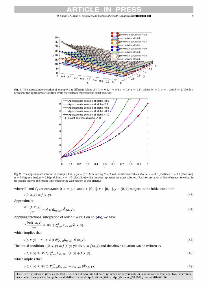
Fig. 1. The approximate solution of example 1 at different values of t (t = 0.2, t = 0.4, t = 0.6, t = 0.8), where M = 7, α = 1 and β = 2. The dotsrepresent the approximate solution while the surfaces represent the exact solution.

Fig. 2. The approximate solution of example 1 at (x, y) = (0.1, 0.1), setting β = 2 and for different values of α i.e. α = 0.6 (red line), α = 0.7 (blue line),α = 0.8 (green line), α = 0.9 (pink line), α = 1.0 (black line) while the dots represent the exact solution. (For interpretation of the references to colour inthis figure legend, the reader is referred to the web version of this article.)

where C1 and C2 are constants, 0 < α ≤ 1, and t ∈ [0, 1], x ∈ [0, 1], y ∈ [0, 1], subject to the initial condition

u(0, x, y) = f (x, y). (45)

Approximate


≈ Ψ (t)KM×M2 Ψ (x, y). (46)

Applying fractional integration of order α w.r.t. t on Eq. (46), we have

Iα∂u(t, x, y)∂tα

≈ Ψ (t)PαTM×MKM×M2 Ψ (x, y),

which implies that

u(t, x, y)− c1 ≈ Ψ (t)PαTM×MKM×M2 Ψ (x, y). (47)

The initial condition u(0, x, y) = f (x, y) yields c1 = f (x, y) and the above equation can be written as

u(t, x, y) ≈ Ψ (t)PαTM×MKM×M2 P(x, y)+ f (x, y), (48)

which implies that

u(t, x, y) ≈ Ψ (t)(PαTM×MKM×M2 + FM×M2)Ψ (x, y). (49)


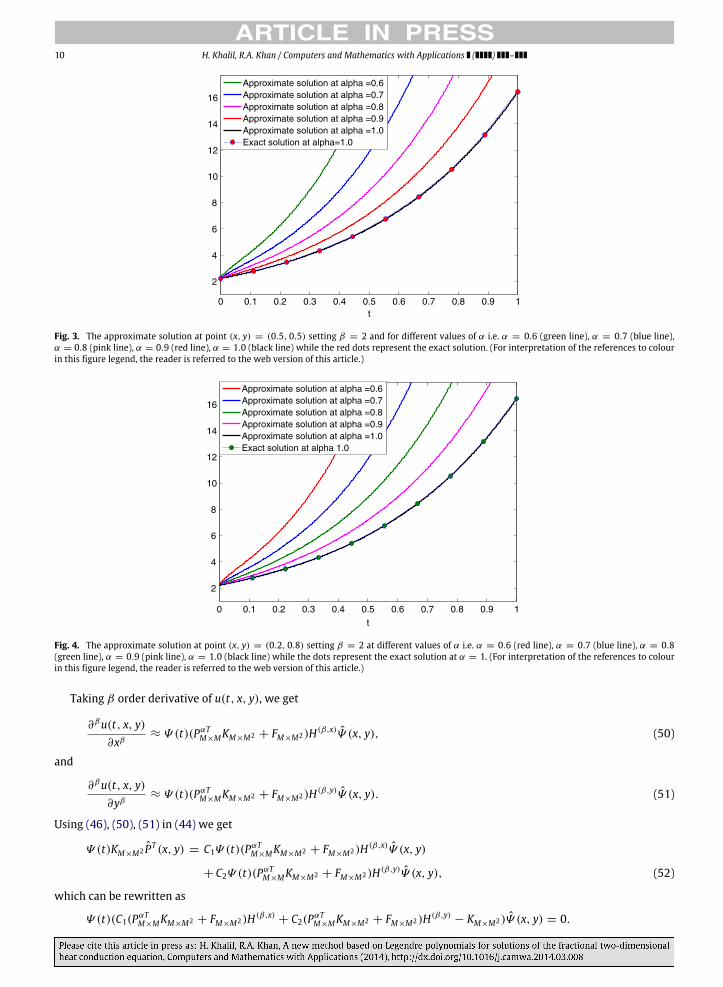
Fig. 3. The approximate solution at point (x, y) = (0.5, 0.5) setting β = 2 and for different values of α i.e. α = 0.6 (green line), α = 0.7 (blue line),α = 0.8 (pink line), α = 0.9 (red line), α = 1.0 (black line) while the red dots represent the exact solution. (For interpretation of the references to colourin this figure legend, the reader is referred to the web version of this article.)

Fig. 4. The approximate solution at point (x, y) = (0.2, 0.8) setting β = 2 at different values of α i.e. α = 0.6 (red line), α = 0.7 (blue line), α = 0.8(green line), α = 0.9 (pink line), α = 1.0 (black line) while the dots represent the exact solution at α = 1. (For interpretation of the references to colourin this figure legend, the reader is referred to the web version of this article.)

Taking β order derivative of u(t, x, y), we get

∂βu(t, x, y)∂xβ

≈ Ψ (t)(PαTM×MKM×M2 + FM×M2)H(β,x)Ψ (x, y), (50)

and


≈ Ψ (t)(PαTM×MKM×M2 + FM×M2)H(β,y)Ψ (x, y). (51)

Using (46), (50), (51) in (44) we get

Ψ (t)KM×M2 PT (x, y) = C1Ψ (t)(PαTM×MKM×M2 + FM×M2)H(β,x)Ψ (x, y)

+ C2Ψ (t)(PαTM×MKM×M2 + FM×M2)H(β,y)Ψ (x, y), (52)

which can be rewritten as

Ψ (t)(C1(PαTM×MKM×M2 + FM×M2)H(β,x) + C2(PαTM×MKM×M2 + FM×M2)H(β,y) − KM×M2)Ψ (x, y) = 0.


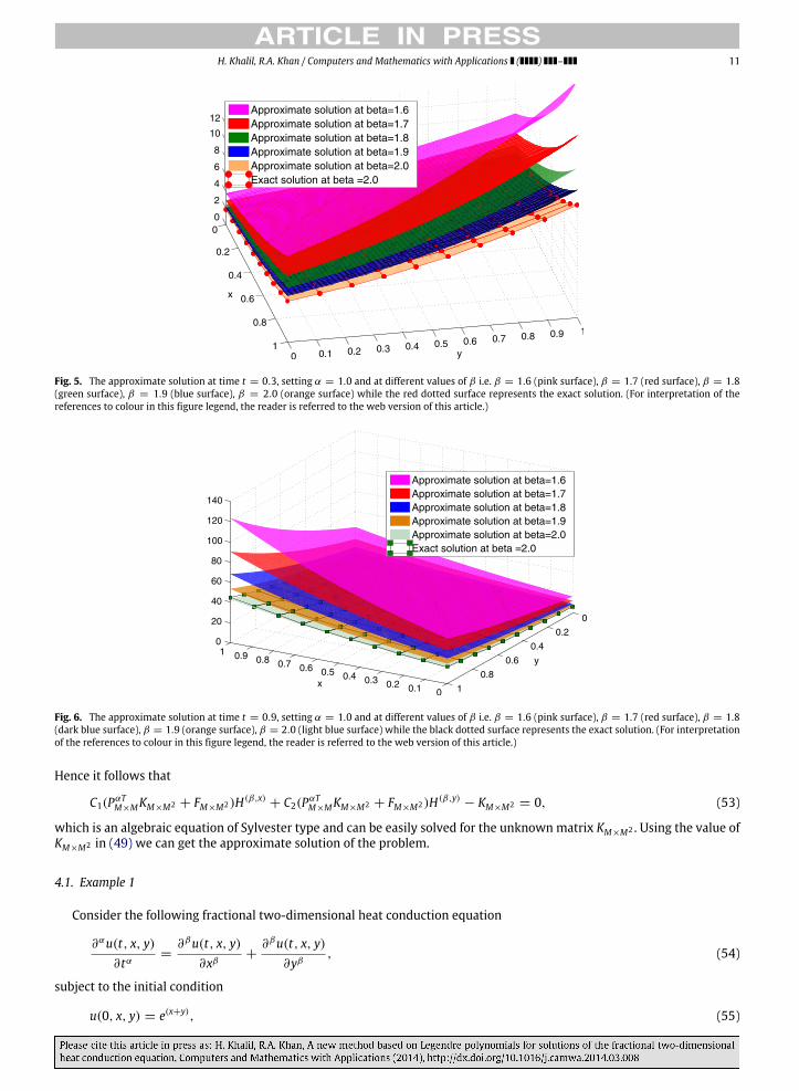
Fig. 5. The approximate solution at time t = 0.3, setting α = 1.0 and at different values of β i.e. β = 1.6 (pink surface), β = 1.7 (red surface), β = 1.8(green surface), β = 1.9 (blue surface), β = 2.0 (orange surface) while the red dotted surface represents the exact solution. (For interpretation of thereferences to colour in this figure legend, the reader is referred to the web version of this article.)

Fig. 6. The approximate solution at time t = 0.9, setting α = 1.0 and at different values of β i.e. β = 1.6 (pink surface), β = 1.7 (red surface), β = 1.8(dark blue surface), β = 1.9 (orange surface), β = 2.0 (light blue surface) while the black dotted surface represents the exact solution. (For interpretationof the references to colour in this figure legend, the reader is referred to the web version of this article.)

Hence it follows that

C1(PαTM×MKM×M2 + FM×M2)H(β,x) + C2(PαTM×MKM×M2 + FM×M2)H(β,y) − KM×M2 = 0, (53)

which is an algebraic equation of Sylvester type and can be easily solved for the unknownmatrix KM×M2 . Using the value ofKM×M2 in (49) we can get the approximate solution of the problem.

4.1. Example 1

Consider the following fractional two-dimensional heat conduction equation


=∂βu(t, x, y)

∂xβ+∂βu(t, x, y)

∂yβ, (54)

subject to the initial condition

u(0, x, y) = e(x+y), (55)


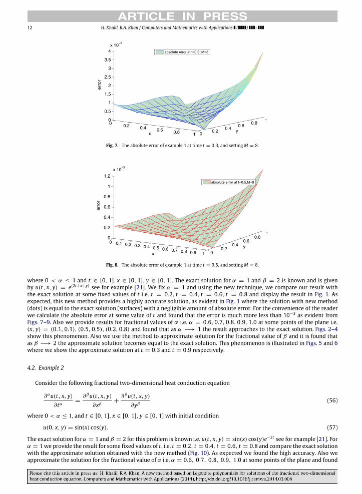
Fig. 7. The absolute error of example 1 at time t = 0.3, and settingM = 8.


where 0 < α ≤ 1 and t ∈ [0, 1], x ∈ [0, 1], y ∈ [0, 1]. The exact solution for α = 1 and β = 2 is known and is givenby u(t, x, y) = e(2t+x+y) see for example [21]. We fix α = 1 and using the new technique, we compare our result withthe exact solution at some fixed values of t i.e. t = 0.2, t = 0.4, t = 0.6, t = 0.8 and display the result in Fig. 1. Asexpected, this new method provides a highly accurate solution, as evident in Fig. 1 where the solution with new method(dots) is equal to the exact solution (surfaces) with a negligible amount of absolute error. For the convenience of the readerwe calculate the absolute error at some value of t and found that the error is much more less than 10−3 as evident fromFigs. 7–9. Also we provide results for fractional values of α i.e. α = 0.6, 0.7, 0.8, 0.9, 1.0 at some points of the plane i.e.(x, y) = (0.1, 0.1), (0.5, 0.5), (0.2, 0.8) and found that as α −→ 1 the result approaches to the exact solution. Figs. 2–4show this phenomenon. Also we use the method to approximate solution for the fractional value of β and it is found thatas β −→ 2 the approximate solution becomes equal to the exact solution. This phenomenon is illustrated in Figs. 5 and 6where we show the approximate solution at t = 0.3 and t = 0.9 respectively.

4.2. Example 2

Consider the following fractional two-dimensional heat conduction equation


=∂βu(t, x, y)

∂xβ+∂βu(t, x, y)

∂yβ(56)

where 0 < α ≤ 1, and t ∈ [0, 1], x ∈ [0, 1], y ∈ [0, 1] with initial condition

u(0, x, y) = sin(x) cos(y). (57)

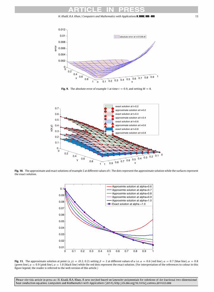
The exact solution for α = 1 and β = 2 for this problem is known i.e. u(t, x, y) = sin(x) cos(y)e−2t see for example [21]. Forα = 1we provide the result for some fixed values of t , i.e. t = 0.2, t = 0.4, t = 0.6, t = 0.8 and compare the exact solutionwith the approximate solution obtained with the new method (Fig. 10). As expected we found the high accuracy. Also weapproximate the solution for the fractional value of α i.e. α = 0.6, 0.7, 0.8, 0.9, 1.0 at some points of the plane and found


Fig. 9. The absolute error of example 1 at time t = 0.9, and setting M = 8.

Fig. 10. The approximate and exact solutions of example 2 at different values of t . The dots represent the approximate solutionwhile the surfaces representthe exact solution.

Fig. 11. The approximate solution at point (x, y) = (0.2, 0.2) setting β = 2 at different values of α i.e. α = 0.6 (red line), α = 0.7 (blue line), α = 0.8(green line), α = 0.9 (pink line), α = 1.0 (black line) while the red dots represent the exact solution. (For interpretation of the references to colour in thisfigure legend, the reader is referred to the web version of this article.)


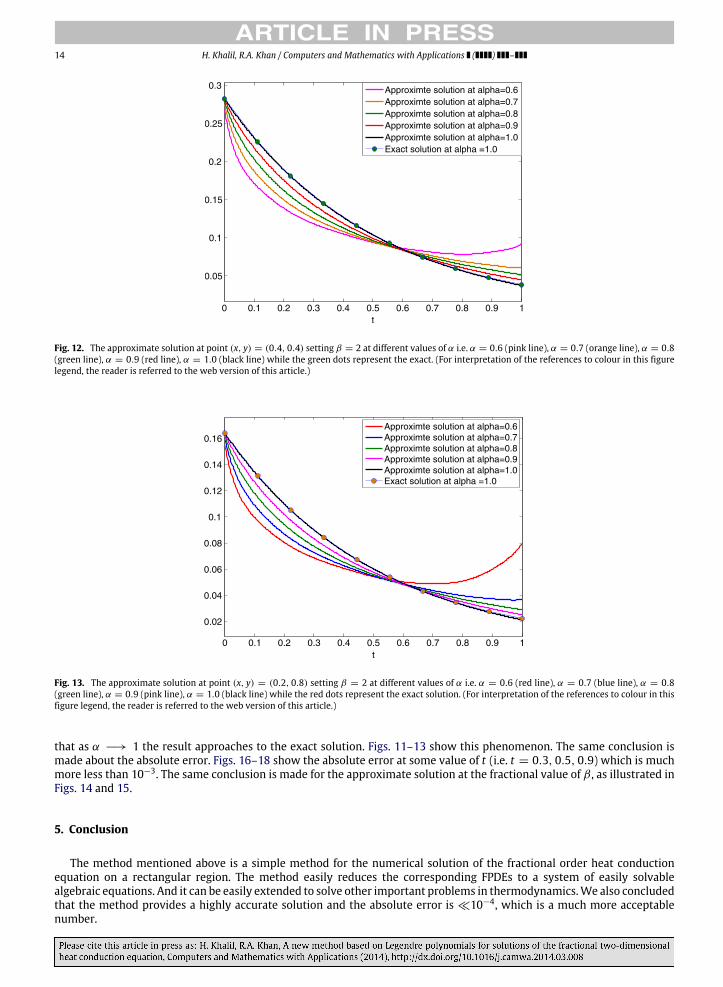
Fig. 12. The approximate solution at point (x, y) = (0.4, 0.4) setting β = 2 at different values of α i.e. α = 0.6 (pink line), α = 0.7 (orange line), α = 0.8(green line), α = 0.9 (red line), α = 1.0 (black line) while the green dots represent the exact. (For interpretation of the references to colour in this figurelegend, the reader is referred to the web version of this article.)

Fig. 13. The approximate solution at point (x, y) = (0.2, 0.8) setting β = 2 at different values of α i.e. α = 0.6 (red line), α = 0.7 (blue line), α = 0.8(green line), α = 0.9 (pink line), α = 1.0 (black line) while the red dots represent the exact solution. (For interpretation of the references to colour in thisfigure legend, the reader is referred to the web version of this article.)

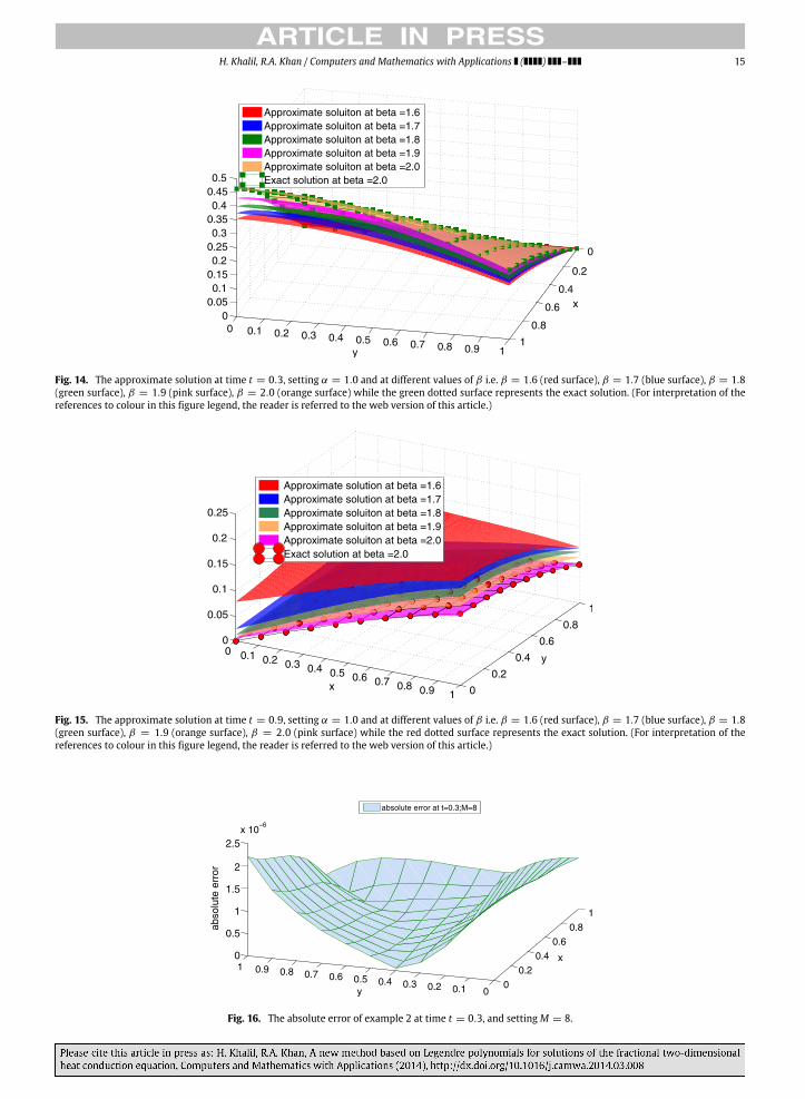
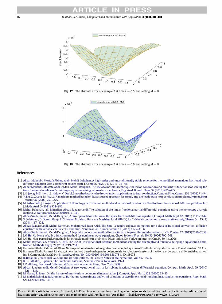
that as α −→ 1 the result approaches to the exact solution. Figs. 11–13 show this phenomenon. The same conclusion ismade about the absolute error. Figs. 16–18 show the absolute error at some value of t (i.e. t = 0.3, 0.5, 0.9) which is muchmore less than 10−3. The same conclusion is made for the approximate solution at the fractional value of β , as illustrated inFigs. 14 and 15.

5. Conclusion

The method mentioned above is a simple method for the numerical solution of the fractional order heat conductionequation on a rectangular region. The method easily reduces the corresponding FPDEs to a system of easily solvablealgebraic equations. And it can be easily extended to solve other important problems in thermodynamics.We also concludedthat the method provides a highly accurate solution and the absolute error is ≪10−4, which is a much more acceptablenumber.


Fig. 14. The approximate solution at time t = 0.3, setting α = 1.0 and at different values of β i.e. β = 1.6 (red surface), β = 1.7 (blue surface), β = 1.8(green surface), β = 1.9 (pink surface), β = 2.0 (orange surface) while the green dotted surface represents the exact solution. (For interpretation of thereferences to colour in this figure legend, the reader is referred to the web version of this article.)

Fig. 15. The approximate solution at time t = 0.9, setting α = 1.0 and at different values of β i.e. β = 1.6 (red surface), β = 1.7 (blue surface), β = 1.8(green surface), β = 1.9 (orange surface), β = 2.0 (pink surface) while the red dotted surface represents the exact solution. (For interpretation of thereferences to colour in this figure legend, the reader is referred to the web version of this article.)

abso

lute

err

or





References

[1] Akbar Mohebbi, Mostafa Abbaszadeh, Mehdi Dehghan, A high-order and unconditionally stable scheme for the modified anomalous fractional sub-diffusion equation with a nonlinear source term, J. Comput. Phys. 240 (2013) 36–48.

[2] Akbar Mohebbi, Mostafa Abbaszadeh, Mehdi Dehghan, The use of a meshless technique based on collocation and radial basis functions for solving thetime fractional nonlinear Schrödinger equation arising in quantum mechanics, Eng. Anal. Bound. Elem. 37 (2013) 475–485.

[3] J.H. Jeong,M.S. Jhon, J.S. Halow, V. Osdol, Smoothed particle hydrodynamics: applications to heat conduction, Comput. Phys. Comm. 153 (2003) 71–84.[4] Y. Liu, X. Zhang, M.-W. Lu, A meshless method based on least squares approach for steady and unsteady state heat conduction problems, Numer. Heat

Transfer 47 (2005) 257–275.[5] M. Akbarzade, J. Langari, Application of Homotopy perturbationmethod and variational iterationmethod to three dimensional diffusion problem, Int.

J. Math. Anal. 5 (2011) 871–880.[6] Mehdi Dehghan, Jalil Manafian, Abbas Saadatmandi, The solution of the linear fractional partial differential equations using the homotopy analysis

method, Z. Naturforsch. 65a (2010) 935–949.[7] Abbas Saadatmandi,Mehdi Dehghan, A tau approach for solution of the space fractional diffusion equation, Comput.Math. Appl. 62 (2011) 1135–1142.[8] S. Soleimani, D. Domiri Ganji, E. Ghasemi, M. Jalaal, Bararnia, Meshless local RBF-DQ for 2-D heat conduction: a comparative study, Therm. Sci. 15 (1)

(2011) 117–121.[9] Abbas Saadatmandi, Mehdi Dehghan, Mohammad-Reza Azizi, The Sinc–Legendre collocation method for a class of fractional convection–diffusion

equations with variable coefficients, Commun. Nonlinear Sci. Numer. Simul. 17 (2012) 4125–4136.[10] Abbas Saadatmandi, Mehdi Dehghan, A Legendre collocationmethod for fractional integro-differential equations, J. Vib. Control 17 (2013) 2050–2058.[11] J.H. He, Xu-Hong Wu, Exp-function method for nonlinear wave equations, Chaos Solitons Fractals 30 (3) (2006) 700–708.[12] J.H. He, Non-perturbative methods for strongly nonlinear problems, Dissertation, De-Verlag im Internet GmbH, Berlin, 2006.[13] Mehdi Deghan, Y.A. Yousefi, A. Lotfi, The use of He’s variational iteration method for solving the telegraph and fractional telegraph equations, Comm.

Numer. Methods Engrg. 27 (2011) 219–231.[14] Hammad Khalil, Rahmat Ali Khan, New operational matrix of inegration and coupled system of Fredholm integral equations. Transformation 10.1: 2.[15] Hammad Khalil, Rahmat Ali Khan, A newmethod based on legender polynomials for solution of system of fractional order partial differential equation,

Int. J. Comput. Math. (2014). http://dx.doi.org/10.1080/00207160.2014.880781. ID: 880781.[16] B. Ross (Ed.), Fractional Calculus and its Applications, in: Lecture Notes in Mathematiucs, vol. 457, 1975.[17] K.B. Oldhalm, J. Spainer, The Fractional Calculus, Academic Press, New York, 1974.[18] I. Podlubny, Fractional Differential Equations, Academic Press, New York, 1999.[19] Abbas Saadatmandi, Mehdi Dehghan, A new operational matrix for solving fractional-order differential equation, Comput. Math. Appl. 59 (2010)

1326–1336.[20] M. Gasea, T. Sauer, On the history of multivariate polynomial interpolation, J. Comput. Appl. Math. 122 (2000) 23–35.[21] M. Mahalakshmi, R. Rajaraman, G. Hariharan, Approximate analytical solutions of two dimensional transient heat conduction equations, Appl. Math.

Sci. 6 (2012) 3507–3518.

http://refhub.elsevier.com/S0898-1221(14)00131-X/sbref1












http://dx.doi.org/doi:10.1080/00207160.2014.880781







Documents

A new method based on Legendre polynomials for solutions of the fractional two-dimensional heat conduction equation