<アジア経済研究所学術研究リポジトリ ARRIDE> http://ir.ide.go.jp/dspace/

Title A New Measurement for International Fragmentation of theProduction Process: An International Input-Output Approach

Author(s) Inomata, Satoshi

Citation IDE Discussion Paper. No. 175. 2008.10

Issue Date 2008-10

URL http://hdl.handle.net/2344/798

Rights

INSTITUTE OF DEVELOPING ECONOMIES

IDE Discussion Papers are preliminary materials circulated to stimulate discussions and critical comments

IDE DISCUSSION PAPER No. 175

A New Measurement for International Fragmentation of the Production Process: An International Input-Output Approach Satoshi Inomata* October 2008

Abstract The paper investigates the possibility of constructing a new measurement for

analysing international fragmentation of the production process. It asserts that the current usage of relevant data, whether the trade shares of parts and components or the index of Vertical Specialisation, is quite unsatisfactory for measuring the phenomenon, since they critically lack the overall perspective of the entire structure of production chains.

The new measurement is formulated such that it captures every aspect of the vertical sequence of production linkages. It is based on the input-output model of Average Propagation Lengths, recently developed by Eric Dietzenbacher and others, which show the average number of production stages that are passed through for an exogenous change in one industry to affect another. By applying this model to the data of the Asian International Input-Output Tables, the index is able to measure the international dimension of production sharing and division of labour in East Asia.

Keywords: international fragmentation, production chains, input-output analysis, Average Propagation Lengths, Asian International Input-Output Tables, East Asia JEL classification: C67, C82, F02, F14, F15 * Director, Microeconomic Analysis Group, Development Studies Centre, IDE

(satoshi_inomata@ide.go.jp)

The Institute of Developing Economies (IDE) is a semigovernmental,

nonpartisan, nonprofit research institute, founded in 1958. The Institute

merged with the Japan External Trade Organization (JETRO) on July 1, 1998.

The Institute conducts basic and comprehensive studies on economic and

related affairs in all developing countries and regions, including Asia, the

Middle East, Africa, Latin America, Oceania, and Eastern Europe. The views expressed in this publication are those of the author(s). Publication does not imply endorsement by the Institute of Developing Economies of any of the views expressed within.

INSTITUTE OF DEVELOPING ECONOMIES (IDE), JETRO 3-2-2, WAKABA, MIHAMA-KU, CHIBA-SHI CHIBA 261-8545, JAPAN ©2008 by Institute of Developing Economies, JETRO No part of this publication may be reproduced without the prior permission of the IDE-JETRO.

1. Introduction During the last few decades there was a flourishing discussion on a new economic phenomenon of international trade; that is, the increasing number of segments in a production process, or production chains, has been rapidly and extensively relocated to different places of different countries. The international fragmentation of the production process caught the interest of many academics and policy-makers alike, and various analytical models were formulated thereafter in order to capture the dynamics of this new economic trend. Prompted by the earlier propositions of Ethier (1982), the theoretical side of international fragmentation underwent significant development through a series of studies in the 1990s. Based on the classic concept of comparative advantage, the theory and its major implications became well established and widely shared. What has lagged behind, however, is an empirical analysis. Although the relevant data has become increasingly available, the methodological aspect of constructing an appropriate measurement has yet to catch up. This paper proposes a new measurement for the international fragmentation of production process, in order to overcome such deficiency and contribute to the development of empirical analysis on the topics of current concern. The paper is organised as follows. The second section briefly reviews previous empirical studies and discusses the possible shortcomings of the measurements employed in those studies. In the third section a new measurement for international fragmentation is introduced, with an explanation of the underlying theoretical model and the basic picture of intercountry input-output data. The fourth section presents the calculation results using the new measurement, and compares the results with other types of indices. The fifth section summarises the discussion. 2. Literature review 2.1 Current methods of measuring international fragmentation In general, the major branch of empirical studies uses either (1) foreign trade statistics [Feenstra & Hanson (1996), Yeats (1998), Ng & Yeats (1999), Jones, Kierzkowski, &

Lurong (2005), Kimura & Ando (2005)] or (2) input-output tables [Campa & Goldberg (1997), Hummels, Ishii, & Yi (2001), Shrestha (2007), Uchida (2008)] as a principal data source. Each type of data has its own advantages and disadvantages, which are more or less reflected in the method of measurement chosen for the analysis of the topic. A representative study of the former category is Ng and Yeats (1999). Following the earlier approach developed in Yeats (1998), it sets forth a comprehensive analysis of production sharing in the East Asian region, using the trade data for parts and components of 60 manufacturing industries. It finds, as of 1996, that the share of the components trade accounted for one-fifth of the whole basket of imports and exports in East Asia. What is even more outstanding is the speed of increase. East Asia’s global exports of components from 1984 to 1996 grew at an annual rate of 15 % compared with 11 % for all manufacturing products. In particular, intra-regional trade rapidly intensified, with its share of total trade almost doubling from 25% to 46 %. Furthermore, the study proposes a new approach for using the Revealed Comparative Advantage index. Usually, the index indicates the international competitiveness of an industry by using export data of the country of concern. Ng and Yeats (1999) instead use the import data for parts and components, in order to illustrate the comparative advantage of a country in assembly operations. The study defines RCAa (“a” for “assembly”) and RCAp (“p” for “production”) as follows.

RCAa = [mr(i)/Mr]/[mw(i)/Mw]*100

RCAp = [xr(i)/Xr]/[xw(i)/Xw]*100

where mr(i): Country R’s imports of good i, Mr: Total imports of country R, mw(i): World’s imports of good i, Mw: Total imports of the World.

The same definitions are applied to x and X for export data (which forms a conventional index of RCA). By comparing these two indices for each country analysed, the study presents a profile of the national production cycle, i.e. whether a country is in the “assembly stage” or the “production stage” of manufacturing products. The study finds that international fragmentation in East Asia has been occurring in a way that confirms the Factor Proportion Theory, in that assembly operations, which are considered to be labour-intensive, are more prevalent in low-income countries like

Indonesia, Thailand and Malaysia, while the high income countries/regions such as Taiwan, Hong Kong and Singapore have already entered the “sunset stage” of assembly operations and are moving towards the production of parts and components. Turning to the application of input-output tables, the first to use such data for analysing international fragmentation was Campa and Goldberg (1997), in which the imported inputs of four industrialised countries, the U.S.A., Canada, the U.K., and Japan, are compared at three points in time. The study examines the impact of external shocks on the domestic production of manufacturing industries. Its argument generally centres around whether a country becomes more vulnerable to external shocks as a result of international fragmentation, and various indices of a country’s “external orientation” are devised for the analysis. The study however fails to make the best use of input-output tables. It only picks up and compares the values of imported inputs shown in the tables, which can claim no methodological advantage over a simple comparison of import data of intermediate goods taken from foreign trade statistics. The strength of an input-output table, and what makes it special, is indeed the information of production linkages that are derived from input-output relations between industries. In this regard, Hummels, Ishii and Yi (2001) present a simple yet tractable usage of input-output data, introducing a narrowly defined concept of international fragmentation. They define their Vertical Specialisation as the amount of intermediate inputs for the production of a good divided by the total output of that good, multiplied by the good’s export value. Put differently, it is the imported contents of an exported item. Within this input-output framework, a country’s Vertical Specialisation is represented in a matrix form as:

VS = uMX

where u is a summation vector, M is an import coefficient matrix, and X is an export vector. The study employs the input-output tables of ten OECD countries with 35 industrial sectors which are compared at two points of time, around 1970 and 1990.1 It shows that the Vertical Specialisation index is increasing in most of OECD countries except Japan, and that it tends to be higher for the countries with small domestic market.

1 The analysis is augmented with the data of Korea, Taiwan, Ireland and Mexico.

These findings have been confirmed more significantly for the East Asian countries in a recent study of Uchida (2008), which utilises the data of the Asian International Input-Output Tables for the years 1975-2000.2 Shrestha (2007) also uses the same data set for an analysis of the East Asian region, though it devises a slightly different framework of Vertical Specialisation. 2.2 The possible shortcomings of the present measurements Although the studies mentioned above have been repeatedly cited and referred to in a number of subsequent researches, a close examination of the concept of international fragmentation reveals that the present methods do not offer satisfactory measurements to describe the phenomenon. The theory of fragmentation predicts that if the production process of a certain final good consists of many segments of production blocks, or has potentials for further segmentation by the change in economies of scales, then there exists a lager opportunity for a fine division of labour that leads to the better allocation of resources and lower marginal cost of production. This is especially true if we allow for access to international markets, since the difference in factor endowments (and hence comparative advantages) are even more prominent across borders.3 It is quite evident, therefore, that the analysis of fragmentation concerns the number of production stages involved in a production process. It is a study to compare the alternative technologies that lead to the production of the same good, between one comprised of few production blocks and another with many.4 The empirical research thus requires an overall perspective for the entire structure of production chains. Not only does the size/magnitude of production linkages matter, but also the “length” of the chains, determined by the number of production blocks therein, provides important information for the analysis. In this respect, foreign trade statistics suffer from a critical drawback for the analysis of fragmentation. While the statistics are undoubtedly the most accessible data for the

2 The tables were constructed by the Institute of Developing Economies, JETRO. 3 See Jones & Kierzkowski (1990), and Deardorff (1998). 4 Deardorff (1998) defines ’fragmentation’ as “the splitting of a production process into two or more steps that can be undertaken in different locations but that lead to the same final product”.

study of international trade, and have become increasingly available for many countries,5 these statistics contain no information on the linkages between industries. The vertical structure of the production process cannot be depicted, which is supposed to be the analytical target of international fragmentation. The import and export values of parts & components offer a suggestion or a “clue” for considering the propensity of international fragmentation, yet it cannot depict the phenomenon per se. The index of Vertical Specialisation, on the other hand, offers significant methodological advances, in the sense that it explicitly incorporates the industrial linkages in its specification of the index. By utilising input-output tables with import matrices, it is able to quantify the international dimension of vertical linkages in the form of import contents embodied in exported items. The index, however, is also explicit in its limitation. Although it refers to the industrial linkage of certain segments of production chains, it cannot trace back the sequence by any more than two consecutive stages of production blocks. Vertical Specialisation, therefore, fails to provide a complete picture of entire production chains, and is bound to give us only a partial indication of the dynamics of international fragmentation.6 3. A new measurement for international fragmentation 3.1 The model In this section, a new measurement for international fragmentation is proposed. The method of constructing the new measurement is based on the model of Average Propagation Lengths, the latest technique of input-output analysis recently developed in Dietzenbacher et al. (2005).

5 The latest version of the harmonised system (version 3, 10 digits) offers approximately 850 categories of items described as “parts”, compared to 60 items in the SITC Revision 2 when Ng and Yeats conducted their study in 1999. 6 Hummels, Ishii and Yi (2001) also presents an alternative model that incorporates the overall domestic production linkages. The model, VS = uM(I-A)-1X where (I-A)-1 is a Leontief Inverse matrix, captures both the direct and indirect effects of the export demand on imports, by allowing domestic circulation of the external impact before it ultimately induces the import of intermediate goods.

This does not however solve the current problem since the Leontief Inverse as it is only gives a consequence of production spillover but cannot refer to its process. All different stages of the production process are “squashed and stamped” into an instantaneous picture of ex post equilibrium. The Leontief Inverse in this setting is just a black box regarding the vertical structure of production linkages.

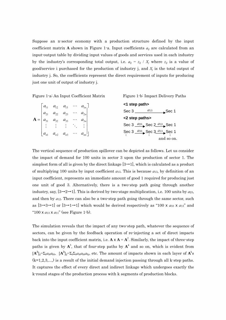
Suppose an n-sector economy with a production structure defined by the input coefficient matrix A shown in Figure 1-a. Input coefficients aij are calculated from an input-output table by dividing input values of goods and services used in each industry by the industry’s corresponding total output, i.e. aij = zij / Xj where zij is a value of good/service i purchased for the production of industry j, and Xj is the total output of industry j. So, the coefficients represent the direct requirement of inputs for producing just one unit of output of industry j.

Figure 1-a: An Input Coefficient Matrix Figure 1-b: Impact Delivery Paths

<1 step path> S

ec 3 Sec 1 a13

<

2 step paths> S

ec 3 Sec 2 Sec 1 Sec 3 Sec 3 Sec : : :

1 and so on.

a23 a12 a33 a13 ⎥

⎥⎥⎥⎥⎥

⎦

⎤

⎢⎢⎢⎢⎢⎢

⎣

⎡

=

nnnnn

n

n

n

aaaa

aaaaaaaaaaaa

321

3333231

2232221

1131211

A

The vertical sequence of production spillover can be depicted as follows. Let us consider the impact of demand for 100 units in sector 3 upon the production of sector 1. The simplest form of all is given by the direct linkage [3→1], which is calculated as a product of multiplying 100 units by input coefficient a13. This is because a13, by definition of an input coefficient, represents an immediate amount of good 1 required for producing just one unit of good 3. Alternatively, there is a two-step path going through another industry, say, [3→2→1]. This is derived by two-stage multiplication, i.e. 100 units by a23, and then by a12. There can also be a two-step path going through the same sector, such as [3→3→1] or [3→1→1] which would be derived respectively as “100 x a33 x a13” and “100 x a13 x a11” (see Figure 1-b). The simulation reveals that the impact of any two-step path, whatever the sequence of sectors, can be given by the feedback operation of re-injecting a set of direct impacts back into the input coefficient matrix, i.e. A x A = A2. Similarly, the impact of three-step paths is given by A3, that of four-step paths by A4 and so on, which is evident from [A2]ij=Σkaikakh，[A3]ij=ΣkΣhaikakhahj, etc. The amount of impacts shown in each layer of Aks (k=1,2,3,...,) is a result of the initial demand injection passing through all k-step paths. It captures the effect of every direct and indirect linkage which undergoes exactly the k-round stages of the production process with k segments of production blocks.

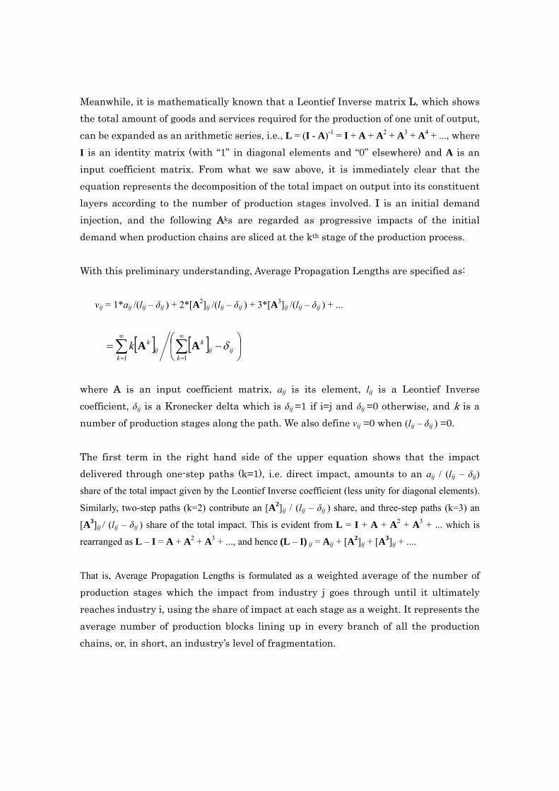
Meanwhile, it is mathematically known that a Leontief Inverse matrix L, which shows the total amount of goods and services required for the production of one unit of output, can be expanded as an arithmetic series, i.e., L = (I - A)-1 = I + A + A2 + A3 + A4 + ..., where I is an identity matrix (with “1” in diagonal elements and “0” elsewhere) and A is an input coefficient matrix. From what we saw above, it is immediately clear that the equation represents the decomposition of the total impact on output into its constituent layers according to the number of production stages involved. I is an initial demand injection, and the following Aks are regarded as progressive impacts of the initial demand when production chains are sliced at the kth stage of the production process. With this preliminary understanding, Average Propagation Lengths are specified as:

vij = 1*aij /(lij – δij ) + 2*[A2]ij /(lij – δij ) + 3*[A3]ij /(lij – δij ) + ...

[ ] [ ] ⎟⎠

⎞⎜⎝

⎛−= ∑∑

∞

=

∞

=ij

kij

k

kij

kk δ11

AA

where A is an input coefficient matrix, aij is its element, lij is a Leontief Inverse coefficient, δij is a Kronecker delta which is δij =1 if i=j and δij =0 otherwise, and k is a number of production stages along the path. We also define vij =0 when (lij – δij ) =0. The first term in the right hand side of the upper equation shows that the impact delivered through one-step paths (k=1), i.e. direct impact, amounts to an aij / (lij – δij)

share of the total impact given by the Leontief Inverse coefficient (less unity for diagonal elements).

Similarly, two-step paths (k=2) contribute an [A2]ij / (lij – δij ) share, and three-step paths (k=3) an

[A3]ij / (lij – δij ) share of the total impact. This is evident from L = I + A + A2 + A3 + ... which is

rearranged as L – I = A + A2 + A3 + ..., and hence (L – I) ij = Aij + [A2]ij + [A3]ij + ....

That is, Average Propagation Lengths is formulated as a weighted average of the number of production stages which the impact from industry j goes through until it ultimately reaches industry i, using the share of impact at each stage as a weight. It represents the average number of production blocks lining up in every branch of all the production chains, or, in short, an industry’s level of fragmentation.

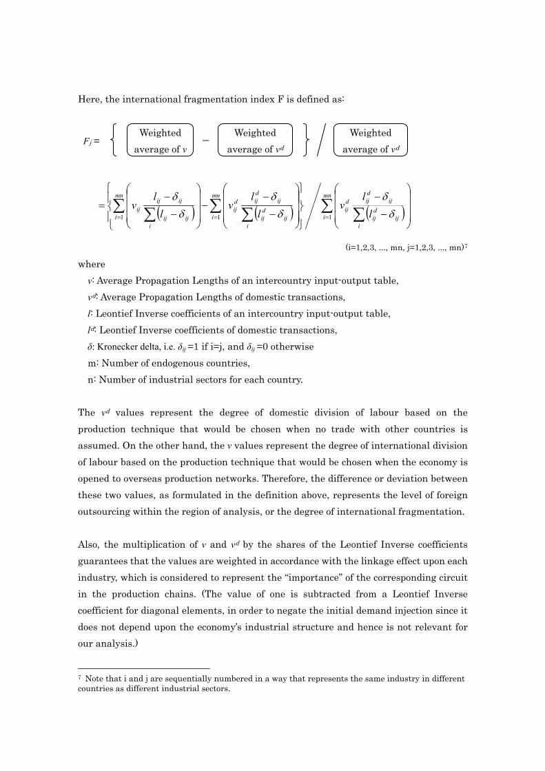
Here, the international fragmentation index F is defined as:

Fj = Weighted

average of v Weighted

average of vd Weighted

average of vd −

( ) ( ) ( )∑ ∑∑ ∑∑ ∑ === ⎟⎟⎟

⎠

⎞

⎜⎜⎜

⎝

⎛

−

−

⎪⎭

⎪⎬

⎫

⎪⎩

⎪⎨

⎧

⎟⎟⎟

⎠

⎞

⎜⎜⎜

⎝

⎛

−

−−

⎟⎟⎟

⎠

⎞

⎜⎜⎜

⎝

⎛

−

−=

mn

ii

ijdij

ijdijd

ij

mn

ii

ijdij

ijdijd

ij

mn

ii

ijij

ijijij l

lv

ll

vl

lv

111 δδ

δδ

δδ

(i=1,2,3, ..., mn, j=1,2,3, ..., mn)7

where v: Average Propagation Lengths of an intercountry input-output table, vd: Average Propagation Lengths of domestic transactions, l: Leontief Inverse coefficients of an intercountry input-output table, ld: Leontief Inverse coefficients of domestic transactions, δ: Kronecker delta, i.e. δij =1 if i=j, and δij =0 otherwise

m: Number of endogenous countries, n: Number of industrial sectors for each country.

The vd values represent the degree of domestic division of labour based on the production technique that would be chosen when no trade with other countries is assumed. On the other hand, the v values represent the degree of international division of labour based on the production technique that would be chosen when the economy is opened to overseas production networks. Therefore, the difference or deviation between these two values, as formulated in the definition above, represents the level of foreign outsourcing within the region of analysis, or the degree of international fragmentation. Also, the multiplication of v and vd by the shares of the Leontief Inverse coefficients guarantees that the values are weighted in accordance with the linkage effect upon each industry, which is considered to represent the “importance” of the corresponding circuit in the production chains. (The value of one is subtracted from a Leontief Inverse coefficient for diagonal elements, in order to negate the initial demand injection since it does not depend upon the economy’s industrial structure and hence is not relevant for our analysis.)

7 Note that i and j are sequentially numbered in a way that represents the same industry in different countries as different industrial sectors.

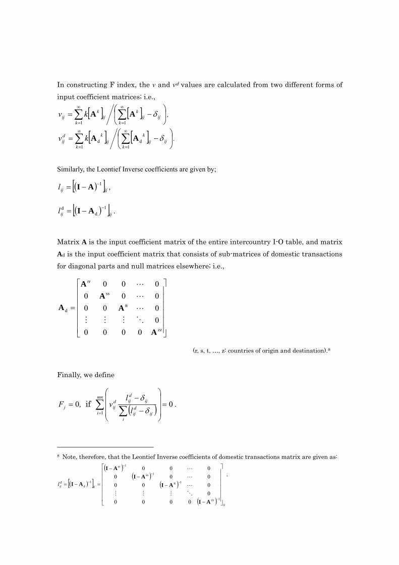
In constructing F index, the v and vd values are calculated from two different forms of input coefficient matrices; i.e.,

[ ] [ ] ⎟⎠

⎞⎜⎝

⎛−= ∑∑

∞

=

∞

=ij

kij

k

kij

kij kv δ

11AA ,

[ ] [ ] ⎟⎠

⎞⎜⎝

⎛−= ∑∑

∞

=

∞

=ij

kij

k

kij

kdij kv δ

1d

1d AA .

Similarly, the Leontief Inverse coefficients are given by;

( )[ ]ijijl 1−−= AI ,

( )[ ]ijijl 1d

d −−= AI .

Matrix A is the input coefficient matrix of the entire intercountry I-O table, and matrix Ad is the input coefficient matrix that consists of sub-matrices of domestic transactions for diagonal parts and null matrices elsewhere; i.e.,

⎥⎥⎥⎥⎥⎥

⎦

⎤

⎢⎢⎢⎢⎢⎢

⎣

⎡

=

zz

tt

ss

rr

d

00000000000000

A

AA

A

A

(r, s, t, …, z: countries of origin and destination).8

Finally, we define

( ) 001

=⎟⎟⎟

⎠

⎞

⎜⎜⎜

⎝

⎛

−

−= ∑ ∑=

mn

ii

ijdij

ijdijd

ijj ll

v,Fδ

δif .

8 Note, therefore, that the Leontief Inverse coefficients of domestic transactions matrix are given as:

( )[ ]

( )( )

( )

( ) ij

ijijl

⎥⎥⎥⎥⎥⎥

⎦

⎤

⎢⎢⎢⎢⎢⎢

⎣

⎡

−

−−

−

=−=

−

−

−

−

−

1zz

1tt

1ss

1rr

1d

d

00000000000000

AI

AIAI

AI

AI

.

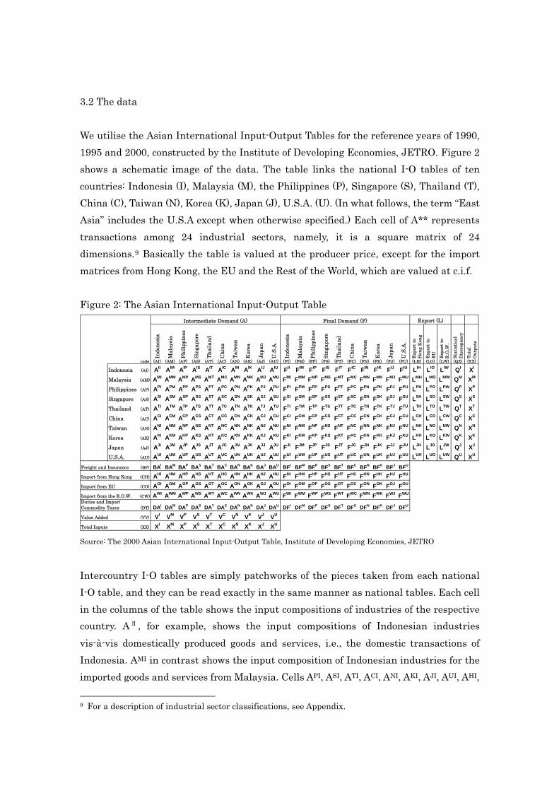
3.2 The data We utilise the Asian International Input-Output Tables for the reference years of 1990, 1995 and 2000, constructed by the Institute of Developing Economies, JETRO. Figure 2 shows a schematic image of the data. The table links the national I-O tables of ten countries: Indonesia (I), Malaysia (M), the Philippines (P), Singapore (S), Thailand (T), China (C), Taiwan (N), Korea (K), Japan (J), U.S.A. (U). (In what follows, the term “East Asia” includes the U.S.A except when otherwise specified.) Each cell of A** represents transactions among 24 industrial sectors, namely, it is a square matrix of 24 dimensions.9 Basically the table is valued at the producer price, except for the import matrices from Hong Kong, the EU and the Rest of the World, which are valued at c.i.f. Figure 2: The Asian International Input-Output Table

Indo

nesi

a

Mal

aysi

a

Phili

ppin

es

Sing

apor

e

Thai

land

Chi

na

Taiw

an

Kor

ea

Japa

n

U.S

.A.

Indo

nesi

a

Mal

aysi

a

Phili

ppin

es

Sing

apor

e

Thai

land

Chi

na

Taiw

an

Kor

ea

Japa

n

U.S

.A.

Exp

ort t

oH

ong

Kon

gE

xpor

t to

EU

Exp

ort t

oR

.O.W

.St

atis

tica

lD

iscr

epan

cyTo

tal

Out

puts

code (AI) (AM) (AP) (AS) (AT) (AC) (AN) (AK) (AJ) (AU) (FI) (FM) (FP) (FS) (FT) (FC) (FN) (FK) (FJ) (FU) (LH) (LO) (LW) (QX) (XX)

Indonesia (AI) AII AIM AIP AIS AIT AIC AIN AIK AIJ AIU FII FIM FIP FIS FIT FIC FIN FIK FIJ FIU LIH LIO LIW QI XI

Malaysia (AM) AMI AMM AMP AMS AMT AMC AMN AMK AMJ AMU FMI FMM FMP FMS FMT FMC FMN FMK FMJ FMU LMH LMO LMW QM XM

Philippines (AP) API APM APP APS APT APC APN APK APJ APU FPI FPM FPP FPS FPT FPC FPN FPK FPJ FPU LPH LPO LPW QP XP

Singapore (AS) ASI ASM ASP ASS AST ASC ASN ASK ASJ ASU FSI FSM FSP FSS FST FSC FSN FSK FSJ FSU LSH LSO LSW QS XS

Thailand (AT) ATI ATM ATP ATS ATT ATC ATN ATK ATJ ATU FTI FTM FTP FTS FTT FTC FTN FTK FTJ FTU LTH LTO LTW QT XT

China (AC) ACI ACM ACP ACS ACT ACC ACN ACK ACJ ACU FCI FCM FCP FCS FCT FCC FCN FCK FCJ FCU LCH LCO LCW QC XC

Taiwan (AN) ANI ANM ANP ANS ANT ANC ANN ANK ANJ ANU FNI FNM FNP FNS FNT FNC FNN FNK FNJ FNU LNH LNO LNW QN XN

Korea (AK) AKI AKM AKP AKS AKT AKC AKN AKK AKJ AKU FKI FKM FKP FKS FKT FKC FKN FKK FKJ FKU LKH LKO LKW QK XK

Japan (AJ) AJI AJM AJP AJS AJT AJC AJN AJK AJJ AJU FJI FJM FJP FJS FJT FJC FJN FJK FJJ FJU LJH LJO LJW QJ XJ

U.S.A. (AU) AUI AUM AUP AUS AUT AUC AUN AUK AUJ AUU FUI FUM FUP FUS FUT FUC FUN FUK FUJ FUU LUH LUO LUW QU XU

Freight and Insurance (BF) BAI BAM BAP BAS BAT BAC BAN BAK BAJ BAU BFI BFM BFP BFS BFT BFC BFN BFK BFJ BFU

Import from Hong Kong (CH) AHI AHM AHP AHS AHT AHC AHN AHK AHJ AHU FHI FHM FHP FHS FHT FHC FHN FHK FHJ FHU

Import from EU (CO) AOI AOM AOP AOS AOT AOC AON AOK AOJ AOU FOI FOM FOP FOS FOT FOC FON FOK FOJ FOU

Import from the R.O.W. (CW) AWI AWM AWP AWS AWT AWC AWN AWK AWJ AWU FWI FWM FWP FWS FWT FWC FWN FWK FWJ FWU

(DT) DAI DAM DAP DAS DAT DAC DAN DAK DAJ DAU DFI DFM DFP DFS DFT DFC DFN DFK DFJ DFU

Value Added (VV) VI VM VP VS VT VC VN VK VJ VU

Total Inputs (XX) XI XM XP XS XT XC XN XK XJ XU

Duties and ImportCommodity Taxes

Intermediate Demand (A) Final Demand (F) Export (L)

Source: The 2000 Asian International Input-Output Table, Institute of Developing Economies, JETRO

Intercountry I-O tables are simply patchworks of the pieces taken from each national I-O table, and they can be read exactly in the same manner as national tables. Each cell in the columns of the table shows the input compositions of industries of the respective country. AⅡ , for example, shows the input compositions of Indonesian industries vis-à-vis domestically produced goods and services, i.e., the domestic transactions of Indonesia. AMI in contrast shows the input composition of Indonesian industries for the imported goods and services from Malaysia. Cells API, ASI, ATI, ACI, ANI, AKI, AJI, AUI, AHI,

9 For a description of industrial sector classifications, see Appendix.

AOI, AWI, indicate the imports from other countries. BA* and DA* give the international freight & insurance and taxes on these import transactions. The 11th column from the left side of the table shows the compositions of goods and services that have gone to the final demand sectors of Indonesia. FII and FMI, for example, show respectively the goods and services produced domestically and those imported from Malaysia that flow into Indonesian final demand sectors. The rest of the column is read in the same manner as for the 1st column of the table. L*H, L*O, L*W are exports (vectors) to Hong Kong, the EU and the Rest of the World, respectively. V* and X* are value-added and total input/output, as seen in the conventional national I-O table. Q* represents the statistical discrepancies in each row. 4. Calculation results 4.1 Results for the international fragmentation in East Asia10 Figure 3 presents the calculation results by industrial sectors for the reference years of 1990, 1995 and 2000. They are aggregate figures for the whole East Asian region (manufacturing sectors only), and the values are averaged across countries using each industry’s gross output as weights. The capital-labour requirement ratio of each industry is given in parentheses below the sector code.11 The industry that showed the highest level of international fragmentation in the year 2000 was “017 Machinery”, while “018 Transport equipment” is catching up very rapidly, with a rate of increase of approximately 49%. These findings conform to our intuition that machinery sectors, especially Electronics and Automobiles, have been playing leading roles in the development of international value chains in East Asia.12 10 In calculating the Average Propagation Lengths, the number of iteration is set at k=10, yet this covers more than 98% of total impacts for most of the industrial sectors. 11 The capital-labour requirement ratio is calculated from the value-added coefficients of the Asian International Input-Output Table using the value-added items “Wage and salary” and “Operating surplus” as proxies. The K/L requirement ratio = ki/wi, where ki and wi are elements of row vectors k(I-A)-1 and w(I-A)-1 for industry i, respectively, and k and w are the value-added coefficient vectors, and A is the input coefficient matrix, of the intercountry I-O table. (Note that the ratio therefore accounts for the factor requirement of the whole range of production chains of an industry.) The values are averaged across countries using each industry’s gross output as weights，and then its period average is taken from the values of 1990, 1995 and 2000. 12 See Oikawa (2008).

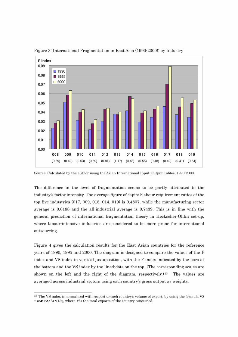
Figure 3: International Fragmentation in East Asia (1990-2000): by Industry

0.00

0.01

0.02

0.03

0.04

0.05

0.06

0.07

0.08

0.09

008 009 010 011 012 013 014 015 016 017 018 019

1990

1995

2000

F index

(0.89) (0.49) (0.53) (0.59) (0.81) (1.17) (0.48) (0.55) (0.48) (0.49) (0.41) (0.54)

Source: Calculated by the author using the Asian International Input-Output Tables, 1990-2000.

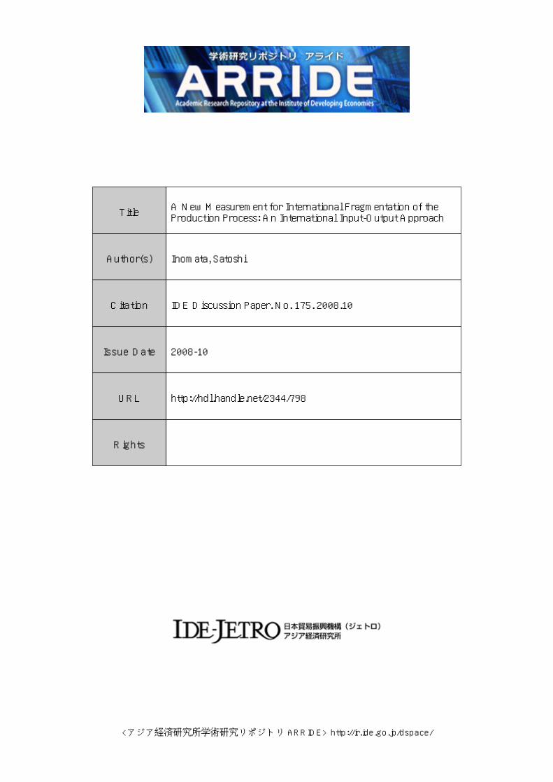
The difference in the level of fragmentation seems to be partly attributed to the industry’s factor intensity. The average figure of capital-labour requirement ratios of the top five industries (017, 009, 018, 014, 019) is 0.4807, while the manufacturing sector average is 0.6188 and the all-industrial average is 0.7439. This is in line with the general prediction of international fragmentation theory in Heckscher-Ohlin set-up, where labour-intensive industries are considered to be more prone for international outsourcing. Figure 4 gives the calculation results for the East Asian countries for the reference years of 1990, 1995 and 2000. The diagram is designed to compare the values of the F index and VS index in vertical juxtaposition, with the F index indicated by the bars at the bottom and the VS index by the lined-dots on the top. (The corresponding scales are shown on the left and the right of the diagram, respectively.) 13 The values are averaged across industrial sectors using each country’s gross output as weights.

13 The VS index is normalised with respect to each country’s volume of export, by using the formula VS = uM(I-A)-1X*(1/x), where x is the total exports of the country concerned.

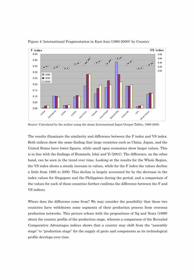
Figure 4: International Fragmentation in East Asia (1990-2000): by Country

0.00

0.05

0.10

0.15

0.20

0.25

0.30

0.35

0.40

0.45

CHINA

INDONESIA

JAPAN

KOREA

MALAYSIA

TAIWAN

PHILIPPIN

ES

SINGAPORE

THAILAND

USA

Whole R

egion

1990

1995

2000

0.00

0.20

0.40

0.60

0.80

VS indexF index

Source: Calculated by the author using the Asian International Input-Output Tables, 1990-2000.

The results illuminate the similarity and difference between the F index and VS index. Both indices show the same finding that large countries such as China, Japan, and the United States have lower figures, while small open economies show larger values. This is in line with the findings of Hummels, Ishii and Yi (2001). The difference, on the other hand, can be seen in the trend over time. Looking at the results for the Whole Region, the VS index shows a steady increase in values, while for the F index the values decline a little from 1995 to 2000. This decline is largely accounted for by the decrease in the index values for Singapore and the Philippines during the period, and a comparison of the values for each of these countries further confirms the difference between the F and VS indices. Where does the difference come from? We may consider the possibility that these two countries have withdrawn some segments of their production process from overseas production networks. This picture echoes with the propositions of Ng and Yeats (1999) about the country profile of the production stage, wherein a comparison of the Revealed Comparative Advantages indices shows that a country may shift from the “assembly stage” to “production stage” for the supply of parts and components as its technological profile develops over time.

Thus it is possible that Singapore from the early 1990s and the Philippines from the mid-1990s onwards started to supply domestically some part of production inputs, which had previously been purchased from overseas producers. Assembly operations may still be a principal job for them, yet they have successfully “internalised” some segments of production chains, possibly of upstream industries, after an intensive learning process of the production technology through participation in international production networks. This possibility, however, can be completely dropped out of the picture drawn by VS index, since it is able to shed a light on only a part of production chains, and, if unfortunate, the “internalised” segments could be the ones positioned beyond its analytical range. The F index, on the other hand, can grasp it as the model of Average Propagation Lengths captures the entire structure of vertical chains at every production stage of every single branch. The difference in the trend of index values, therefore, seems to reflect the difference in the analytical range of the F index and VS index.

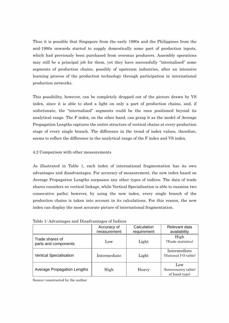
4.2 Comparison with other measurements As illustrated in Table 1, each index of international fragmentation has its own advantages and disadvantages. For accuracy of measurement, the new index based on Average Propagation Lengths surpasses any other types of indices. The data of trade shares considers no vertical linkage, while Vertical Specialisation is able to examine two consecutive paths; however, by using the new index, every single branch of the production chains is taken into account in its calculations. For this reason, the new index can display the most accurate picture of international fragmentation. Table 1: Advantages and Disadvantages of Indices Accuracy of

measurement Calculation requirement

Relevant data availability

Trade shares of parts and components Low Light

High (Trade statistics)

Vertical Specialisation Intermediate Light Intermediate

(National I-O table)

Average Propagation Lengths High Heavy Low

(Intercountry table) of Isard type)

Source: constructed by the author

On the other hand, the new index suffers from the practical problems of data availability and the burden it puts on calculation. Perhaps the calculation constraints are not as severe as ten years ago in terms of data processing capacity. However, since many researchers today are more used to working on a spreadsheet rather than with a mainframe, the users of Microsoft Excel will find out that the current version of the software does not allow the inversion of a matrix with considerably high order. The calculation of the Average Propagation Lengths for a full-scale intercountry I-O table could be a nasty job for them. The problem of data availability is even more salient. Foreign trade statistics are available for most of the UN member countries on a quarterly or monthly base. Input-output tables are also available for an increasing number of countries since the data constitutes the core apparatus of the System of National Accounts, (although the release frequency is much less than the other types of statistics; usually once in every five years). An intercountry input-output table, by contrast, is such a rarity. To the author’s knowledge, the full-scale, Isard-type multicountry tables have been constructed in the past only for the European and East Asian regions.14 One must thus admit, therefore, that for the experiment on East Asia presented in this section, it has only been the rare case of a happy marriage between the Average Propagation Lengths and the Asian International I-O Table that enabled this full-range analysis of international fragmentation. The above notwithstanding, nowadays there has been a rapid development in data processing capacity, and methodological advances for estimating intercountry I-O tables.15 The previous disadvantages are expected to become less and less inhibiting for researchers, and hence there is sufficient reason to acknowledge a greater application potential of the new measurement in the years to come. 5. Conclusion This paper investigated the possibility of constructing a new measurement for the

14 Asian International Input-Output Tables (1975-2000), by the Institute of Developing Economies, JETRO; EC-6 table (1959-75) by Schilderinck, EC-7 table (1977) by Langer, EC-7 tables (1965-85) by Linder and Oosterhaven, EU-10 tables (1985, 95) and EU-11 tables (1995, 2000) by Yoshinaga. 15 Especially the method developed through the collaboration of the University of Groningen and the Institute of Developing Economies, JETRO, provides a useful reference. See Oosterhaven et al. (2007).

analysis of international fragmentation. It pointed out that the current methods, whether using the trade shares of parts and components or the index of Vertical Specialisation, are unsatisfactory for measuring the phenomenon, since they critically lack an overall perspective of the entire structure of production chains. The new measurement is formulated such that it captures every aspect of the vertical sequence of production linkages. It is based on the input-output model of Average

Propagation Lengths, which gives the average number of production stages passed through by an exogenous change in one industry until it ultimately affects another. By applying this model to the data of intercountry input-output tables, this study demonstrated that the index is able to measure the international dimension of production sharing and division of labour. The results of the empirical study showed that in East Asia the machinery sector achieved the highest level of international fragmentation during the period between 1990 and 2000, while the cross-national analysis revealed that some countries like Singapore and the Philippines have gradually withdrawn from international production sharing in the region, possibly moving towards the phase of vertical integration of the production process. A comparison with other types of indices clarified the advantages and disadvantages of the new measurement, but it is concluded that the method will overcome the current problems in the near future and is expected to open up better prospects for the analysis of international fragmentation.

<References> Campa, J. and Goldberg, L. (1997), “The Evolving External Orientation of

Manufacturing Industries: Evidence from Four Countries”, NBER Working Paper no.5919.

Deardorff A.V. (1998), ‘Fragmentation in Simple Trade Models’, Research Seminar in International Economics, Discussion Paper No.422.

Dietzenbacher, E., Romero, L., and Bosma, N.S. (2005), ‘Using Average Propagation Lengths to Identify Production Chains in the Andalusian Economy’, Estudios de Economia Aplicada 23: 405-422.

Ethier,W.J. (1982), “National and International Returns to Scale in the Modern Theory of International Trade”, American Economic Review, 389-405.

Feenstra R.C. & G.H. Hanson (1996), “Foreign Investment, Outsourcing, and Relative Wages”, In: R.C. Feenstra, G.M. Grossman & D.A. Irwin (eds.), The Political Economy of Trade Policy; Papers in Honor of Jagdish Bhagwati, The MIT Press, Cambridge, 89-127.

Jones R.W. & H. Kierzkowski (1990), “The Role of Services in Production and International Trade: A Theoretical Framework”, In: R.W. Jones & A. O. Krueger (eds), The Political Economy of International Trade, Basil Blackwell, Oxford, 31-48.

Jones R., H. Kierzkowski, & C. Lurong (2005), ‘What Does Evidence Tell Us About Fragmentation and Outsourcing?’, International Review of Economics and Finance, Vol. 14, 305-316.

Hummels D., J. Ishii, & K-M. Yi (2001), ‘The Nature and Growth of Vertical Specialization in World Trade’, Journal of International Economics, Vol. 54, 75-96.

Kimura F. & M. Ando (2005), ‘Two-dimensional Fragmentation in East Asia: Conceptual Framework and Empirics’, International Review of Economics and Finance, Vol. 14, 317-348.

Ng F. & A. Yeats (1999), ‘Production Sharing in East Asia; Who Does What for Whom, and Why?’, Policy Research Working Paper 2197, The World Bank, Washington.

Oosterhaven J., Stelder D., and Inomata S. (2007), ‘Evaluation of Non-Survey International IO Construction Methods with the Asian-Pacific Input-Output Table’, IDE Discussion Papers No.114, IDE-JETRO.

Oikawa, H. M. (2008), ‘International Value Distribution in Asian Electronics and Automobile Industries: An Empirical Value Chain Approach’, IDE Discussion Papers No.172, IDE-JETRO.

Shrestha N. (2007), ‘Multi Country Vertical Specialization Dependence: A New Approach to the Vertical Specialization Study’, Hi-Stat Discussion Paper No. 208, Hitotsubashi University, Tokyo.

Uchida Y. (2008), ‘Vertical Specialization in East Asia: Some Evidence from East Asia Using Asian International Input-Output Tables from 1975 to 2000’, Chosakenkyu-Houkokusho, IDE-JETRO.

Yeats A.J. (1998), ‘Just How Big is Global Production Sharing?’, Policy Research Working Paper 1871, The World Bank, Washington.

Asian International Input-Output Table, 1990., IDE-JETRO. Asian International Input-Output Table, 1995., IDE-JETRO. Asian International Input-Output Table, 2000., IDE-JETRO.

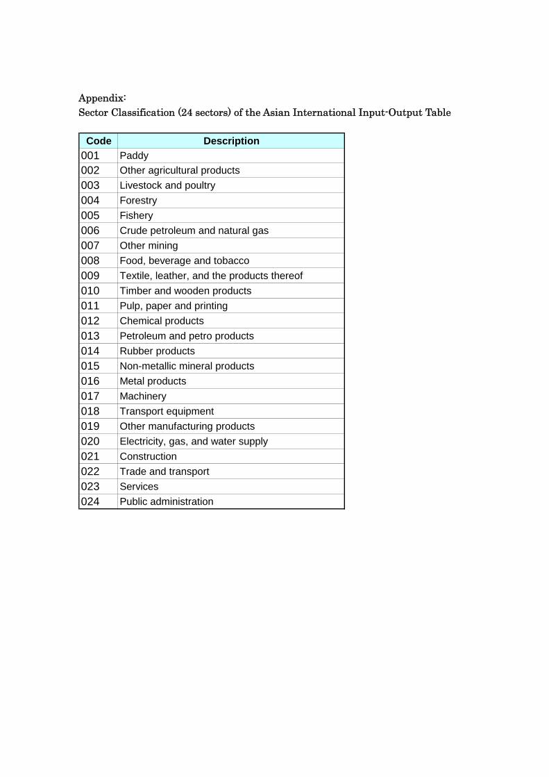
Appendix: Sector Classification (24 sectors) of the Asian International Input-Output Table

Code Description001 Paddy002 Other agricultural products003 Livestock and poultry004 Forestry005 Fishery006 Crude petroleum and natural gas007 Other mining008 Food, beverage and tobacco009 Textile, leather, and the products thereof010 Timber and wooden products011 Pulp, paper and printing012 Chemical products013 Petroleum and petro products014 Rubber products015 Non-metallic mineral products016 Metal products017 Machinery018 Transport equipment019 Other manufacturing products020 Electricity, gas, and water supply021 Construction022 Trade and transport023 Services024 Public administration