Portland State University Portland State University

PDXScholar PDXScholar

Engineering and Technology Management Faculty Publications and Presentations Engineering and Technology Management

1-1-1997

A New Measure of Baseball Batters Using DEA A New Measure of Baseball Batters Using DEA

Timothy R. Anderson Portland State University, tim.anderson@pdx.edu

Gunter P. Sharp Georgia Institute of Technology - Main Campus

Follow this and additional works at: https://pdxscholar.library.pdx.edu/etm_fac

Part of the Engineering Commons

Let us know how access to this document benefits you.

Citation Details Citation Details Anderson, Timothy R. and Sharp, Gunter P., "A New Measure of Baseball Batters Using DEA" (1997). Engineering and Technology Management Faculty Publications and Presentations. 19. https://pdxscholar.library.pdx.edu/etm_fac/19

This Post-Print is brought to you for free and open access. It has been accepted for inclusion in Engineering and Technology Management Faculty Publications and Presentations by an authorized administrator of PDXScholar. Please contact us if we can make this document more accessible: pdxscholar@pdx.edu.

A New Measure of Baseball Batters Using DEA

Timothy R. Anderson

Gunter P. Sharp

Department of Industrial and Systems Engineering

Georgia Institute of Technology, Atlanta, Georgia 30332-0205

Data Envelopment Analysis (DEA) is used to create an alternative to

traditional batting statistics called the Composite Batter Index (CBI).

Advantages of CBI over traditional statistics include the fact that players are

judged on the basis of what they accomplish relative to other players and

that it automatically accounts for changing conditions of the game that raise

or lower batting statistics. Historical results are examined to show how the

industry of baseball batting has matured and potential uses of CBI are

discussed.

The application of baseball suggests that random variation may have

an effect on CBI. We investigated this effect by creating noisy data sets

based on actual data sets and then compared the results, which revealed a

negative bias in the majority of cases. We then present and test an extension

to DEA for mitigating this effect of noise in evaluating a batter’s true “skill.”

Keywords: DEA, noise, baseball

2

0. Introduction

This paper starts by describing an interesting application of data envelopment

analysis (DEA) for evaluating baseball batters. First, a historical background on baseball

statistics is provided. Next, the DEA-based measure called the composite batter index

(CBI) is explained. Since CBI is based on DEA, it is an inherently relative measure and

has several advantages over traditional baseball statistics.

Next, CBI scores are computed historically for the years 1901 to 1993 in both the

American and National Leagues, (AL, NL), resulting in 186 different analyses. The

changing distributions of the scores are related to changes in the game. In particular, a

case is made that the “industry of baseball batting” can be said to be “maturing.” In later

years there are more CBI league leaders and a higher percentage of league leaders. The

same sort of historical analysis could be used to evaluate the “maturity” of other

industries such as automobile manufacturing by examining the number and distribution

of efficient manufacturers.

The last issue raised is that of the effect of noise. CBI is designed to measure

productivity or “how much a player produced in a year.” Another item of interest is

measuring the “skill” of a batter. First, simulation results demonstrate that using CBI to

estimate skill yields biased results. Since baseball batting is a stochastic process, the

number of hits a batter gets is not necessarily a perfect reflection of his skill. This

differentiation between estimating “productivity” and “skill” is important. More

important than the fact that a batter’s productivity score may be subject to this random

variation or “noise” is the fact that he is being compared on a relative measure to his

peers, all of whom also are subject to this noise. Once the importance of this noise

3

problem is established, a new procedure for reducing the effect of noise in DEA (and

therefore CBI) is described. Simulation results verify that this noise correction extension

to DEA can significantly reduce bias and mean squared error in estimating a batter’s skill

via CBI.

1. Background on Baseball Statistics

1.1. Fixed Weight Statistics

Baseball batting statistics can generally be categorized as one of two types,

traditional fixed weights and derived fixed weights. Examples of traditional fixed weight

statistics include the number of home runs (HR), batting average (BA), and slugging

average (SLG). In each case, a simple formula is used to calculate the statistic. These

statistics are usually the most popular with fans because they are the easiest to calculate

and understand. It is widely accepted though that these simple statistics do not provide

an accurate measure of player.

Operations researchers and baseball researchers have shown that more accurate

formulas can be determined in a variety of ways such as historical records and

simulation. These alternative measures are classified as derived fixed weight measures.

During the preceding thirty years, a variety of approaches have been used to analyze the

problem of determining weights. One method was to examine how a player's probability

distribution of hits affected the number of runs scored by a team in an inning. Examples

of these and other approaches can be found (Lindsey, 1963) (Cover and Keilers, 1977)

(Thorn and Palmer, 1984).

1.2. Variable Weight Statistics

4

A third type of baseball batting statistic, variable weight, was first developed

using DEA by (Mazur, 1995). Mazur used a zero dimensional input, three output model

which consisted of just batting average, home runs, and runs-batted-in (RBI). Mazur's

goal was to demonstrate the use of DEA for evaluating sports and not to provide a new

method for the baseball community to adopt. He justifies these outputs as being the triple

crown criteria and that they are three of the most commonly cited statistics by baseball

fans and writers. He goes on to state that other inputs and outputs could be used.

Mazur achieves his goal but the model would not be accepted by baseball

statisticians. Runs-batted-in is largely a function of the number of players on base when

the player bats and whether or not the pitcher decides to pitch around the hitter.

Therefore, it may depend more on a hitter's place in the batting order and the skills of his

teammates than on his own skills. Home runs are related in part to the number of at-bats

which is omitted from Mazur's model. Batting average does not reflect the value of

walks but this could be easily fixed by replacing this measure with on-base-percentage

(OBP). Despite questions about the model, Mazur accomplished his goal of

demonstrating the use of DEA in sports.

Another interesting application of DEA to baseball was in analyzing salary equity

(Howard and Miller, 1993). The authors used a 29-input, single-output model of salary.

As inputs, the model included official at-bats, runs-batted-in, runs scored, and fielding

average among others on both a single season and career total basis. The number of

seasons played was included as an input while walks were not. Although the choice of

inputs might be questioned in an evaluation of player skill or productivity, the inputs

used are often perceived as positives by the public and team management and a case

5

could therefore be made to include them in the author's model with regards to evaluating

salary equity. This model would not be an appropriate basis upon which to evaluate

overall player productivity though.

2. Advantages of DEA Based Approaches

A DEA based approach (or other variable weight method) has several advantages

over other techniques. One advantage is that it can provide a relative measure of a

player’s skill compared to players throughout the league. For example, when home runs

became easier to hit, traditional fixed weight statistics make it appear as if many players

have suddenly become much more skilled.

The classic example of this was the introduction of the so called lively baseball

along with rule changes affecting spitballs and scuffed balls in the late 1910s. The home

run totals immediately increased dramatically. It would be a mistake to attribute this

increase entirely to an increase in player skill. If it became “twice as easy” to hit a home

run in 1920, then a batter should hit twice as many home runs or else make up for it in

other areas. Other situations where this is useful would be when league expansion dilutes

pitching quality, when park sizes change, and when rule changes or reinterpretations

occur.

A numerical example illustrates the tendency of fixed weight measures to be

deceptively applied to cross era comparisons. It might be tempting to say that Bill Terry

was a much better hitter in 1930 when he hit 0.401 than was Carl Yastrzemski who hit

0.301 in 1968, even though they both led their respective leagues. This overlooks the

fact that they played in different eras under vastly different circumstances. In fact, the

league-wide batting average in 1930 was 0.312 while the AL average in 1968 was only

6

0.238. This means that Yastrzemski hit almost the same percentage above the league-

wide average as Bill Terry did (Gould, 1986). This led to extensions of the traditional

fixed weight methods such as relative batting average.

3. The CBI Model

3.1. DEA Formulation

First it is necessary to explain the model. The CBI model consists of one input

and five outputs. The input X is plate appearances, which is the number of official at-

bats plus the number of walks (also known as a base-on-balls or BB). Sacrifice flies and

sacrifice bunts are excluded from consideration at this time, but they could easily be

added for a variation of CBI. Hit-by-pitch values were excluded because the batter

usually has no intention getting hit by a hard object traveling at 90 miles/hour. The

outputs Y are the number of walks, singles, doubles, triples and home runs.

An input oriented CCR primal formulation was used for determining DEA

efficiency scores (Charnes, Cooper, and Rhodes, 1978). The standard CCR formulation

assumes constant returns to scale. This is a reasonable assumption in this application

because doubling the number of inputs (plate appearances) should result in double the

number of outputs (hits and walks.) A standard linear programming formulation of DEA

is given in Eq. 1 and is explained in more detail in a variety of sources such as (Seiford

and Thrall, 1990).

7

min ,

. . ,

' ,

, .

s t Y Y

X X

free

0

0 0

0

(1)

DEA determines a score for each player ranging between 0 and 1.0 to indicate

his productivity relative to the rest of the league. For example, if a player receives a

score of = 0.8, this means that some other hitter or combination of hitters in the league

could have produced at least as many of every type of hit in 20% fewer plate

appearances. Players receiving a score of 1.0 are considered “league-leaders” since they

could not be surpassed by any combination of other players in fewer opportunities or

plate appearances. The vector is a set of virtual multipliers. It describes the

combination of league leaders equals or exceeds the player studied.

3.2. Dominance Transformation

Initial results showed that some players were classified as league-leaders strictly

on the basis of an ability to obtain singles or walks. Although this could be quite

acceptable, further examination of these results showed that occasionally some of these

player evaluations were unreasonable since certain players were able to hit enough longer

hits to overcome a deficit in shorter hits and surpass these shorter hitting specialists.

A good illustration of this was in the National League in 1992. Andy van Slyke

and Tony Gwynn were both found to be efficient by DEA:

Player (1992) PA 1b 2b 3b HR BB

8

Tony Gwynn 566 129 27 3 6 46 Andy van Slyke 672 128 45 12 14 58

Basically, Tony Gwynn had a higher number of singles per plate appearance

(129/566) than any other player. On the other hand, Andy van Slyke had more walks,

doubles, triples, and home runs per plate appearance than Gwynn. In fact, Gwynn's

superiority at hitting singles was smaller than van Slyke's cumulative advantage at hitting

doubles, triples, and home runs:

129

566

128

672

45 12 14

672

27 3 6

5660 0046

.

Since van Slyke could have chosen to stop at first base instead of continuing on to

second on those hits, it is reasonable to conclude that longer hits require more skill than

singles. From a manager’s point of view, they are also more valuable. Therefore, it is

reasonable to conclude that van Slyke was actually more productive than Tony Gwynn.

This suggests a dominance relationship among the types of hits.

The dominance transformation of hits was performed as a preprocessing step by

simply adding each type of output (walk or hit) to the number of longer hits by that

player. Home runs were therefore left unchanged. The output of triples became the sum

of triples and home runs; doubles became the sum of doubles, triples, and home runs;

singles became the sum of singles, doubles, triples, and home runs. A walk was treated

as a type of hit inferior to a single, since it has less opportunity for runner advancement.

This meant that the walks output became the number of walks plus singles, doubles,

triples, and home runs.

9

The connection between the principle of dominance and the aggregation of

outputs is fully described in (Ali, Cook, and Seiford, 1991). It should be noted that this

aggregation technique has been shown to be valid only in the case of strict ordinal

relations. This means that hitting a home run is more difficult than a triple, rather than

“at least as difficult” as a triple.

The dominance relationship generally reduced the number of league leaders by

about fifty percent. All later analyses include this dominance relationship. The resulting

model and results are referred to as the Composite Batter Index or CBI.

4. Analysis Results

Separate CBI analyses were conducted on both the American League (AL) and

the National League (NL) for the years 1901 to 1993 (Thorn and Palmer, 1993). These

186 analyses provide interesting trend information and an ability to check the

reasonableness of the results. Historical results are shown for the AL in figures 1, 2, and

3. Only players with 350 or more at-bats with a single team in a season were included in

the analysis so that full time players were not compared against people that played the

equivalent of a half season or less. Hitters that played significantly less than a full season

such as platoon players, unknown rookies, and pitchers trying to hit could make

comparisons with full-time players unrealistic and were therefore excluded.

In 1993 the AL had five CBI league leaders: Frank Thomas, Juan Gonzalez, John

Olerud, Carlos Baerga, and Ken Griffey Jr. Meanwhile, the NL had only two league

leaders, due to the unusually dominating seasons of Barry Bonds and Andres Galarraga.

4.1. Apparent Trends

10

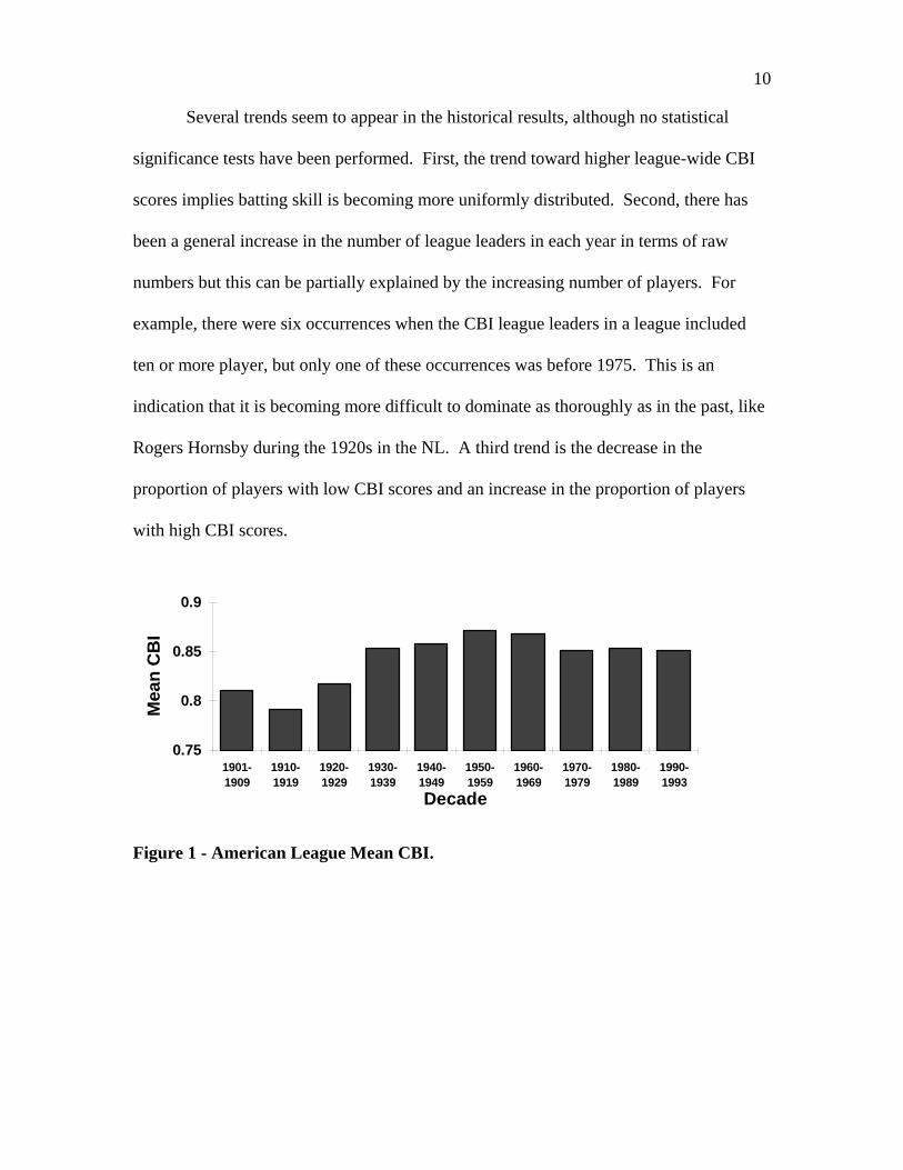
Several trends seem to appear in the historical results, although no statistical

significance tests have been performed. First, the trend toward higher league-wide CBI

scores implies batting skill is becoming more uniformly distributed. Second, there has

been a general increase in the number of league leaders in each year in terms of raw

numbers but this can be partially explained by the increasing number of players. For

example, there were six occurrences when the CBI league leaders in a league included

ten or more player, but only one of these occurrences was before 1975. This is an

indication that it is becoming more difficult to dominate as thoroughly as in the past, like

Rogers Hornsby during the 1920s in the NL. A third trend is the decrease in the

proportion of players with low CBI scores and an increase in the proportion of players

with high CBI scores.

0.75

0.8

0.85

0.9

1901-1909

1910-1919

1920-1929

1930-1939

1940-1949

1950-1959

1960-1969

1970-1979

1980-1989

1990-1993

Decade

Mea

n C

BI

Figure 1 - American League Mean CBI.

11

0

12

3

4

56

7

1901-1909

1910-1919

1920-1929

1930-1939

1940-1949

1950-1959

1960-1969

1970-1979

1980-1989

1990-1993

Decade

Pla

yers

per

Yea

r

Figure 2 - Average Number of CBI League Leaders (AL) per Year.

0

0.1

0.2

0.3

0.4

0.5

1901-1909

1910-1919

1920-1929

1930-1939

1940-1949

1950-1959

1960-1969

1970-1979

1980-1989

1990-1993

Decade

Fra

ctio

n o

f P

laye

rsw

ith

Hig

h/L

ow

CB

I %CBI >= 90

%CBI<=75

Figure 3 - Changing Distribution of CBI Scores over Time.

These results agree with observations by various researchers using more

traditional approaches (Gould, 1986). Gould found that the league standard deviation in

batting averages has dramatically and consistently declined since the turn of the century.

This helps explain why it has been so long since there has been a 0.400 hitter. As

variation decreases, a player must be a higher number of standard deviations above the

12

mean to reach the elusive 0.400 figure since rules have been changed to keep the league-

wide mean batting average near 0.270.

Only two players were ever determined to be the only league leader in a given

year: Rogers Hornsby (1922 and 1925) and Carl Yastrzemski (1967). Not surprisingly,

both players also received triple crowns in those years and would therefore have been the

only leaders based on Mazur's measure. More surprisingly, other triple crown recipients,

such as Lou Gehrig, Ted Williams, and Mickey Mantle, were never the sole league leader

on the basis of CBI.

4.2. Potential Application to Other Industries

It may be possible to generalize such historical trends and apply them to other

areas. In the early stage of an industry the efficiency scores of the entire industry might

be determined by only a few companies with technologies that work much better than

those of their competitors. Over time the technological advantage of the original

companies may dissipate as their competitors improve their operations. Graphically, this

could be visualized as other companies approaching or helping to form the efficiency

frontier. Figures 4 and 5 illustrate these general trends in relation to efficiency frontiers.

Figure 4 - Early Stage of an Industry.

13

Figure 5 - Mature Stage of an Industry.

The world automobile industry could be a good example of this industrial cycle.

In the 1940s and 1950s some of the most efficient car producers in world were in Detroit.

By the 1970s Japanese companies, such as Toyota, Honda, and Nissan had, not only

caught up with the American companies but also surpassed them in many ways by use of

techniques such as just-in-time production. The 1980s and 1990s have seen a frantic race

by the American companies to catch up. The result is that Ford and Chrysler may once

again lie on the efficiency frontier. Similar examples could be determined for other

industries such as ship building.

This type of historical analysis could be extended to indicate the maturity of an

industry or the diffusion of technologies. Applications could then be found in the area of

business and technology forecasting.

5. Effects of Noise

5.1. Motivation

A player receiving a low CBI score may try to rationalize his score by saying that

the frontier players had “lucky” seasons. The difference between a league leader and

another player with just a high CBI could be a single swing of the bat.

14

This can also be seen by thinking of a league with only ten identically skilled

players and a simplified CBI model that only used home runs as the only output.

Through simple random variation, there would typically be one player with more home

runs per plate appearance than any other player. The other nine players would have

lower CBI scores despite having identical skill. If we tried to use CBI to estimate the

relative skill of the ten players, the ten player league would have a mean CBI < 1, and

this value would therefore be a biased estimator of skill. This differentiation between

measuring productivity and underlying skill is important: in many applications skill

would be of more interest than relative production during a period of time. For example,

a baseball general manager may want a measure of skill in determining trade possibilities

to improve her team for the next season.

5.2. Simulating Noise

The effect of noise on DEA measures has not been fully addressed and has been

typically discussed with regards to strictly theoretical data sets. The application of

baseball batting provides a rich area in which to examine the effects of simple random

variation. Towards this end, the effects of noise on CBI were investigated. First, we

wanted to estimate how much of an effect noise could have on the data. This was done

by taking an actual data set, perturbing it with noise, and then comparing the CBI results

between the actual original data set and the noisy data set. Since baseball batting can be

reasonably approximated as a multinomial process, the noisy data set was generated as a

multinomial random variable by using event probabilities from the original data set.

15

5.3. Results

Analyses were conducted using nine different data sets, with the results illustrated

in figure 6. The mean CBI bias induced by noise was negative in the majority of the

cases. The typical bias was approximately -3% for the years examined. The average

mean squared error was about 0.004.

-0.04

-0.02

0

0.02

0.04

0.06

1910 1920 1930 1940 1950 1960 1970 1980 1990

Year

Mea

n B

ias

Figure 6 - Effect of Artificial Noise on Actual Data Sets. Mean bias of CBI scores.

16

Output 1

Output 2

Observed Efficiency Frontier

True Efficiency Frontier

Figure 7 - Example of Noise Biasing the Efficiency Frontier. The circle represents the

player's (or firm's) "true" skill. The lines represent the effect of noise and the end of the

line is then the observed data point.

Since the perturbed data set is multinomial with large N (at least 350), the change

in the data will be approximately symmetrically distributed with a mean of about zero.

The tendency of symmetrically distributed noise to lower efficiency scores by raising the

frontier is illustrated in figure 7. Clearly, cases can be generated where noise will lower

the efficiency frontier too and this occurred in two of the years studied. A positive mean

CBI bias may occur more frequently in applications with different noise distributions.

5.4. Noise Correction

A procedure has been developed and tested for reducing the effects of noise as

described in figure 8. Basically, the procedure consists of adjusting the observed data set

of players (or DMUs) to use in forming the virtual players against which the actual

observed player is compared.

17

1. Read input matrix (vector), X, and output matrix, Y, for all players X AB + BB for player 1 AB + BB for player 2

Y

walks for player 1 walks for player 2

singles for player 1 singles for player 2

doubles for player 1 doubles for player 2

triples for player 1 triples for player 2

home runs for player 1 home runs for player 2

2. Set Y0 equal to column i of Y 3. Derate outputs Y to form Z by use of statistical transformation for all players

except player i. For example, for player 1, the transformation would operate as the following:

X[player 1] (% walks for player 1) (1- % walks for player 1)

X[player 1] (% singles for player 1) (1- % singles for player 1)

X[player 1] (% doubles for player 1) (1- % doubles for player 1)

X[player 1] (% triples for player 1)(1- % triples for player 1)

X[player 1] (% home runs for player 1) (1- % home runs for player 1)

[ ]

[ ] [ ] [ ]

player npq

Z player Y player c player

1

1 1 1

4. Aggregate outputs to form the dominance relationship between the hits and walks. For example, in the case of player i, the aggregation would operate in the following manner:

Z player' [ ]

Z[player 1, walks] + Z[player 1, singles] + Z[player 1, doubles]

+ Z[player 1, triples] + Z[player 1, home runs] Z[player 1, singles] + Z[player 1, doubles]

+ Z[player 1, triples] + Z[player 1, home runs]Z[player 1, doubles] + Z[player 1, triples] + Z[player 1, home runs]

Z[player 1, triples] + Z[player 1, home runs]

Z[player 1, home runs]

1

5. Perform standard DEA with input X and output Z' upon player i.

Figure 8 - Procedure for Computing CBI of Player i with Statistical Extension.

A variety of methods could be used for adjusting the observed data set. We used

a simple adjustment method based on derating the observed data set by a fractional

multiple (c-value) of each player's standard deviation for each multinomial output. Given

the "true" data set, it is possible to find a c-value that will eliminate noise bias and reduce

18

the noise-induced mean squared error. Although these are interesting results, it is an

insufficient test since it relies on unobservable information (the "true" player skills.) The

optimal c-value is in part a function of the distribution of the data set.

5.5. Evaluation of Noise Correction

To test this procedure of correcting for noise, the nine years of data analyzed

earlier to show the effects of noise were examined in an attempt to mitigate the noise

influence. Before we could use the statistical extension, we needed to find an appropriate

c-value for each year. This required the creation of several extra data sets for each year.

The actual data set, designated set A, was assumed to represent the true skill of the

players. Data set B was created by adding multinomial noise to data set A, and then it

was treated as the observed data set. Data set C was created by adding multinomial noise

to data set B and was then used to "tune" the adjustment method by finding a c-value that

eliminated the noise bias in C relative to B. The c-values showed considerable variation

so 100 different data set C’s were generated and the mean c-value was determined and

used in the statistical extension procedure.

19

0.00

0.05

0.10

0.15

0.20

0.25

0.30

0.35

1910 1920 1930 1940 1950 1960 1970 1980 1990

Year

Mea

n c

-val

ue

Figure 9 - Mean c-value for Each Year.

The mean c-value (as shown in figure 9) was then used to adjust data set B, since

in general the distribution of data set C was similar to B. Note that a negative mean c-

value would call for increasing the values in the comparison set. This could be

appropriate in certain applications with significant asymmetric noise but since this

application had symmetric noise such correction would be inappropriate. Therefore

when the mean c-value was negative, a value of zero was used. This occurred once in the

nine years examined. The fact the recommended mean c-value increased as the number

of players in the league (see table 1) increased highlights the possible effect of noise in

large data set DEA problems.

20

Before Correction After CorrectionYear Players Mean Bias MSE Mean c Mean Bias MSE1910 49 -0.0329 0.0056 0.0000 -0.0329 0.00561920 56 0.0080 0.0039 0.1437 0.0200 0.00451930 49 -0.0342 0.0042 0.1549 -0.0200 0.00251940 59 -0.0104 0.0056 0.2176 0.0105 0.00411950 58 -0.0245 0.0040 0.2647 0.0012 0.00331960 50 -0.0357 0.0045 0.2808 -0.0039 0.00311970 76 -0.0216 0.0045 0.3258 0.0078 0.00401980 98 0.0551 0.0065 0.2921 0.0850 0.01101990 103 -0.0137 0.0032 0.2792 0.0135 0.0031

Table 1 - Results of Statistical Extension Procedure on Actual Data Sets with

Artificial Noise.

The mean c-value was then used to derate data set B. As shown in figure 10 and

table 1, the statistical correction improved the results in the majority of the years studied

on the basis of both mean bias and mean-squared-error. In the one case where a c-value

of zero was used, the statistically extended CBI analysis was identical to a regular CBI

analysis.

21

-150%

-100%

-50%

0%

50%

100%

1910 1920 1930 1940 1950 1960 1970 1980 1990

Year (American League)

Imp

rove

men

tBias

MSE

Figure 10 - Improvement Due to Statistical Extension.

It may be possible to improve the CBI noise correction results by applying

different statistical transformations (or derating methods) in step 3 of figure 8. The

statistical transformation used here was tailored to baseball batting but other applications

of DEA may be able to use different methods of derating to reduce noise bias. Although

the noise correction procedure may not be possible in all DEA applications, it does

illustrate the potential benefits of the statistical correction for noise and the need for

further work.

6. Conclusion

DEA was used to develop a new measure of baseball batter performance. This

measure, the composite batter index (CBI), is defined as the percentage of plate

appearances that would be required for the best virtual player to produce at least as much

as the player studied. Since power hitters tend to be compared to other power hitters and

contact hitters with other contact hitters, it provides a good measure of how well players

22

fulfill their roles on teams. It automatically adjusts to different conditions such as the

dead ball and lively ball eras by being an inherently relative measure. Analyses were

performed on actual historic baseball statistics for every year from 1901 to 1993, and

trends showing a maturation of the industry were discussed. CBI could be easily

extended to incorporate other factors such as home park and position played.

This application of DEA could also be used as an intuitive introduction to DEA

modeling. DEA is a powerful tool with many subtleties, but this power and flexibility

also bring the potential for modeling errors. For example, this application highlights the

importance of carefully examining the initial analysis results. As would be expected, this

examination revealed the need for ordinal relations between the outputs in this

application.

Next, it was demonstrated that DEA efficiency scores tend to be negatively biased

by noise that is approximately symmetrically distributed with a zero mean. This led to

the development of a procedure for extending DEA to correct for noise in the data sets.

The procedure calls for comparing each player (or DMU) against a derated data set of

other DMUs. This derating was performed by a statistical (or stochastic) transformation.

Different transformations could be applied in this step depending on the application. The

results of the noise mitigation extension to DEA show promise but also indicate that the

statistical transformation step needs refinement.

23

Acknowledgments

This material is based upon work supported under a National Science Foundation

Graduate Research Fellowship. This work used modified DEA subroutines provided by

the Material Handling Research Center (Hackman and Platzman, 1990).

24

References

Ali, A. I., W. D. Cook, and L. M. Seiford (1991), "Strict vs. Weak Ordinal Relations for Multipliers in Data Envelopment Analysis," Management Science, 37, 6. Charnes, A., Cooper, W.W., and Rhodes, E. (1978), "Measuring the Efficiency of Decision Making Units," European Journal of Operational Research, 2, 6. Cover, T. M. and C. W. Keilers, (1977), "An Offensive Earned-Run Average for Baseball," Operations Research, 25, 5. Gould, S. J. (1986), "Entropic Homogeneity Isn't Why No One Hits .400 Any More," Discover, 7, 8. Hackman, S. T. and L. Platzman (1990), WEA, Computer program for calculating DEA, sponsored by the Material Handling Research Center, Atlanta, GA. Howard, L. H. and J. L. Miller (1993), “Fair pay for fair play: estimating pay equity in professional baseball with data envelopment analysis," Academy of Management Journal, 36, 4. Lindsey, G. R. (1963), "An Investigation of Strategies in Baseball," Operations Research, 11, 4. Mazur, M. J. (1995), "Evaluating the Relative Efficiency of Baseball Players?" Data Envelopment Analysis: Theory, Methodology and Applications, Charnes, Cooper, Lewin, and Seiford, editors, Boston, MA: Kluwer Academic Press. Seiford, L. M. and R. M. Thrall (1990), "Recent Developments in DEA: The Mathematical Programming Approach to Frontier Analysis," Journal of Econometrics, 46. Thorn, J. and P. Palmer (1984), Hidden Game of Baseball, New York, NY: Doubleday. Thorn, J. and P. Palmer (1993), Total Baseball, 3rd Ed., New York, NY: HarperCollins.