A New Dynamic Mesh Method Applied to the Simulation of Selective Laser Melting

Kai Zeng, Deepankar Pal, Nachiket Patil, Brent Stucker

Department of Industrial Engineering, University of Louisville

Abstract

The process of Selective Laser Melting (SLM) involves the moving of a laser beam across a

powder bed to melt material layer by layer. From the standpoint of modeling, this simple

procedure is complicated to capture accurately. SLM involves very high laser intensity values, on the

order of 1010 W/m2 and a Heat Affected Zone (HAZ) that is orders of magnitude less than the

dimensions of the platform. Many computational models have been developed to study

temperature evolution in SLM, but most of these models only simulate a small part of the problem

with a fine mesh or the entire problem using a coarse mesh to avoid the computational burdens of

meshing the full problem with a fine mesh. In order to accurately capture the details of

temperature evolution anywhere in a full-sized part located anywhere in the build platform, in an

efficient manner, a new dynamic moving mesh method has been developed and implemented in

both ANSYS and in a unique Matlab code. This dynamic mesh has been shown to provide significant

computational enhancements over other solution methodologies, while enabling fine-scale

solutions anywhere in the domain space. A detailed comparison between various ways of solving

the SLM problem has been carried out to compare modeling approaches.

Introduction

Additive Manufacturing (AM) technologies have been improved, re-innovated and extended

tremendously since the idea of layer-by-layer fabrication from a CAD model was first developed [1].

As one of the most promising processes, SLM has been successfully applied to aerospace,

automotive, biomedical and other areas and shows great potential for application to additional

industrial problems [2]. As a result, there is a strong demand for SLM quality assurance metrics and

accurate simulation tools capable of predicting density, deformation, dimensions, mechanical

properties, microstructure, etc. Since laser heat energy is used to locally melt powder material, an

understanding of heat transfer in SLM is critical for properly simulating and controlling the process

to enable quality assurance and reproducibility.

Melt pool formation via a laser with high energy density is one of the most important

features driving the thermomechanics of the SLM process. Melt pool formation with short dwelling

times is accompanied with various other spatio-temporal thermal phenomena in the powder bed.

The surface tension induced on the surface of melt pool pulls adjacent unmolten powder, dragging

it into the melt pool[3]. This leads to rough surfaces either causing rake (blade) jams or aesthetically

unpleasing surface textures in the finished part. The melt pool size and its aspect ratio (L/d statistic

of the melt pool) are critical surface tension variables which affect to balling [4]. A complete and

thorough understanding of melt pool formation is therefore fundamental to further improvements

of the SLM process and fabricated products using this technology.

549

Accurate and controlled thermal profiles are a key to better control of melt pool dynamics.

A review of various methods for modeling & monitoring thermal profiles can be found in the

literature [5]. The FEM and thermal monitoring systems were identified as the two most common

ways of studying the melt pool and its evolution dynamics. Several FEM models have been

developed to study thermal distribution in SLM [6-11]. The Gaussian model for a heat source was

adopted in all of these models. Among those models, meshes used in [9, 11] are uniformly gridded

with grid sizes larger than the laser beam diameter, which doesn’t enable accurate modeling of the

Gaussian heat source and raises questions about the accuracy of the predictions. In addition, when

representing a large enough domain to capture part-size thermal phenomena with a mesh fine

enough to accurately represent the heat source, a huge number of nodes and elements must be

incorporated in the 3D model. This added overhead requires significant computational resources

and very high solution times. In [6-8, 10], various non-uniform meshes have been used to represent

the powder or Heat Affected Zones (HAZ). They have limitations as they represent the domain

either in 2 D or by using traditional adaptive refinements which restrict interfacial constraints

between fine and coarse nodes and element connectivity. In this paper, a FEM dynamic meshing

model has been developed to solve the tradeoff of accuracy and computing time using a mapped

fine-coarse (local-global) sub-modeling approach. The current model has been constructed in ANSYS

and a complete comparison against another model [12] coded in MATLAB is discussed as well.

Governing equation and boundary conditions

Heat energy is transferred and dissipated in four main modes when a laser beam hits the

powder bed surface in SLM; those are reflection, conduction, convection and radiation. For a typical

SLM machine such as EOS M270, fabrication takes place inside a closed build chamber purged using

an inert gas like Argon. The heat transfer process can be described by governing equation (1) which

follows the Fourier thermal principle [13].

λ(T)∇2T + q = ρ(T)c(T)∂T

∂t (1)

The substrate is preheated to a certain temperature prior to fabrication (typically 353K in an

EOS M270 machine). The prescribed temperature is described in equation (2) as an initial condition

of the problem.

T(x, y, z, 0) = T0 (2)

Equation (3) describes the connective boundary condition. Heat convection happens

between the powder bed surface and the surrounding environment.

−λ(T)∂T

∂z|z=H = h(T − Te) (3)

Assuming no heat loss at the bottom surface of the substrate, a thermal boundary condition

becomes:

T(x, y, 0, t) = T0 (4)

Where T is the temperature, λ the conductivity coefficient, ρ the density, c the heat capacity coefficient, q the internal heat, T0 the powder bed initial temperature, Te the environment

550

temperature, and h is the convective heat transfer coefficient. All x,y and z notations are according to the ASTM F2921 standard for denoting directions inside an Additive manufacturing machine.

The external heat flux q has been assumed to be a Gaussian heat flux (5):

q =2P

πr02 e

−2r2

r02

(5)

Where P is the laser power, 𝑟0 is the spot radius and r denotes the radial distance. Considering the porosity of the bed, the laser beam has a chance of penetrating into the

powder in the –z direction until it decays [14]. Penetration depends on the wavelength of laser beam and the porosity of the powder [15]. In this paper this penetration is ignored and the heat flux is modeled as a surface based boundary condition with Gaussian quadrature.

Material properties

The SLM process fabricates parts by melting the powder material in a layer by layer fashion.

Material transitions through an iterative cycle (powder bed to bulk-molten continuum to solid bulk

to remelting) several times very quickly due to multiple nearby passes of the laser beam and the

addition of subsequent layers. In this paper, Ti6Al4V powder is studied since it is a commonly used

material in SLM. Material properties such as λ, ρ and c have been varied with temperature, leading

to a non-linear thermal response. In addition, the latent heat of fusion and vaporization are

considered during phase changes. The enthalpy which is defined in equation (6) in ANSYS has been

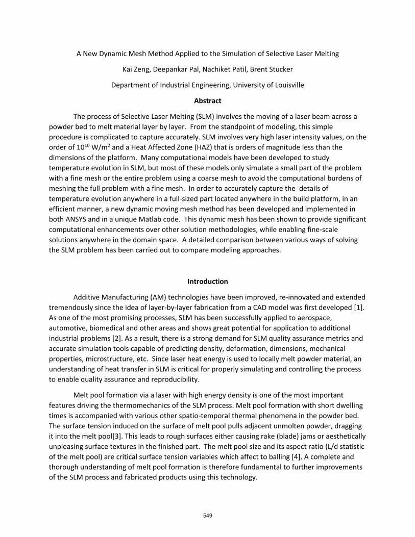
used to account for the latent heat of fusion and vaporization and Figure 1 shows the curve of

enthalpy with respect to temperature [16]. The phase change region is actually a very small zone

with little thermal variation, however the energy has an abrupt change because of the phase or

state transition.

𝐸𝑛𝑡ℎ𝑎𝑝𝑙𝑦 = ∫ ρ(T)c(T)dT (6)

Figure 1 Enthalpy vs Temperature curve

551

In order to compare the current results with results shown in [12], all the relevant

parameters including material properties, process parameters and mesh density have been kept the

same. The thermal conductivity and volumetric heat capacity of the Ti6Al4V can be found from [12].

All the other parameters are summarized in table 1.

Table 1: Process parameters used in the model

Process parameters

Laser power 180w Laser beam diameter 100μm

Scanning speed 1250mm/s Hatch space 100μm

Absorption rate 0.35

Dynamic meshing model

In order to simulate dynamic thermal evolution in SLM and to overcome the difficulties in model

size and computation speeds, a dynamic moving mesh strategy has been developed in ANSYS using its

functionality of sub-modeling. There are two commonly used ways of thermal modeling the SLM

problem. The first uses a uniform mesh and applies a moving heat flux to calculate the thermal history

[9, 11] in which either the model size is small or the element size is big. The other is to try to reduce the

number of element by strategies such as applying a local fine mesh in the laser beam area [6-8, 10].

However, these models usually illustrate the thermal distribution of only one spot rather than

continuous evolution of temperature. The model introduced in this paper is able to simulate thermal

evolution with time and its distribution in space by dynamically moving the mesh shown in figure 2

according to the scan pattern information.

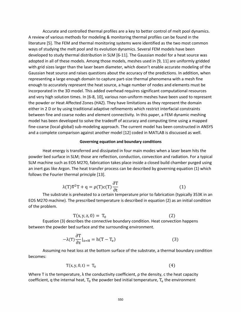
The domain used for simulating this problem is a 1x1x1.5mm 3 Dimensional cuboid. Figure 2

only illustrates the meshing strategy in the XY plane which is extruded in the –z direction. Since the

laser beam diameter is usually very small (100µm), it is the regime with highest thermal gradients and

therefore only a fine mesh with sub-beam diameter element size used for this zone is able to produce

near-accurate results beneficial for fully capturing the problem. Therefore, a fine mesh has been created

for the zone in which the laser beam and its neighboring HAZ zone has been included. A relatively coarse

mesh has been employed in the surrounding areas. This meshing strategy has advantages over previous

strategies by reducing the number of elements, enabling a fully 3D solution and enabling a higher

fidelity solution near the melt pool and HAZ so that the overall thermal distribution prediction has a

more correct slope when predicting thermal variations in the high gradient regions. The black lines in

figure 2 illustrate the xy domain of the model, the thick red box lines represent the HAZ zone and the

inner red box shows the zone of laser beam exposure. The mesh density in this model is the same as

that shown in [12]. Figure 3 shows one of the traditional scan patterns of the laser beam in SLM, which

has been applied in the model. The laser beam, which is located within the inner red box, moves and

follows the track shown in figure 3. In addition, the thick red box, which includes the HAZ, also moves

with the laser beam. The geometry of the model and corresponding boundary conditions are updated

step by step and has been coded using the ANSYS APDL.

552

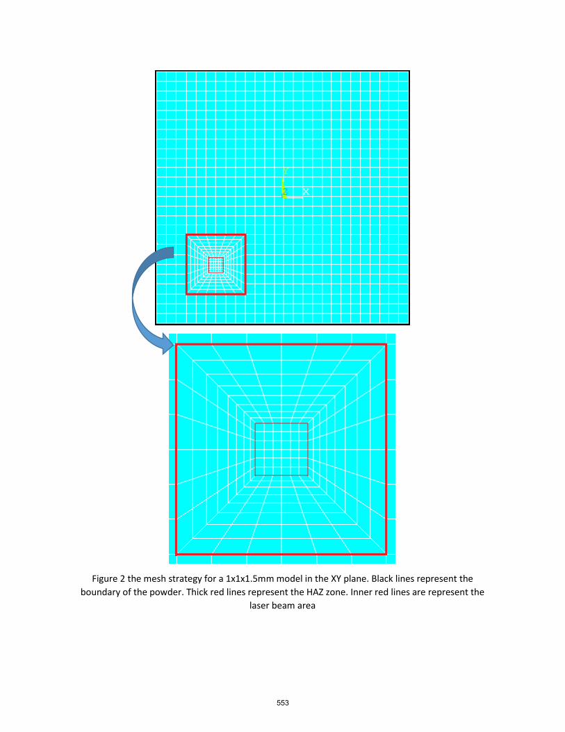
Figure 2 the mesh strategy for a 1x1x1.5mm model in the XY plane. Black lines represent the

boundary of the powder. Thick red lines represent the HAZ zone. Inner red lines are represent the

laser beam area

553

Results and Discussion

The thermal problem arising during SLM processing of Ti6Al4V with parameters from table 1 has

been simulated using the dynamic mesh. The results are shown in Figures 4, 6 and 7. In figure 4 using

the scan pattern shown in figure 3, the melt pool in several locations has been plotted. The melt pool

shows different shapes at different locations, as can be seen in figure 4. The melt pool at the initial

scanning position A is a circular thermal snapshot. With laser beam motion along the first track, the

melt pool slowly transforms to the shape shown at position B. The melt pool shape approaches to a

stable steady state shape by the end of the track and it changes to a different shape at position C when

the laser beam completes a scan vector and turns back for a new track. The melt pool shape will reach a

similar stable state as in the previous track, similar to position C in the new scan vector. Figure 5 shows a

typical SLM melt pool image for comparison [17].

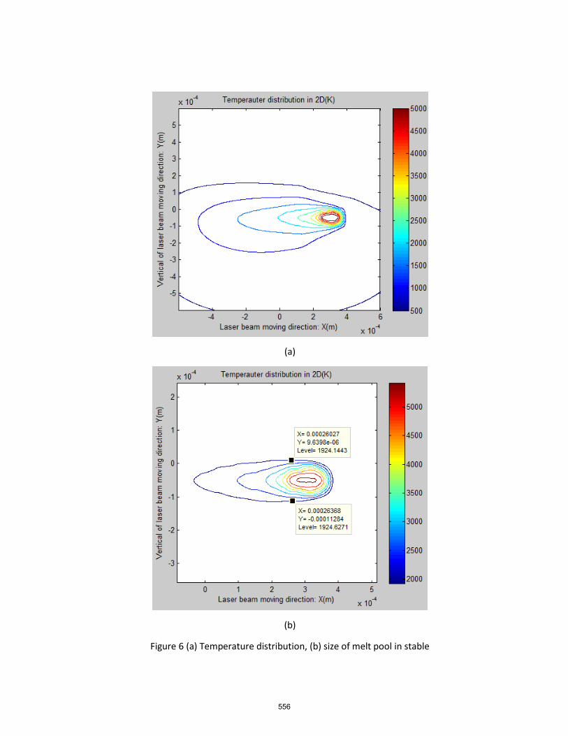
Figure 6(a) shows both the thermal distribution and a stable melt pool size and other low

temperature thermal contours at the center of the powder bed in the third layer. The low temperature

thermal contours are asymmetric due to the solidified bulk on one side and powder on the other side.

The stable melt pool width is about 112µm and its length is about 360µm which can be approximated

from thermal markers shown in figure 6(b). The stable melt pool shows symmetry with respect to the

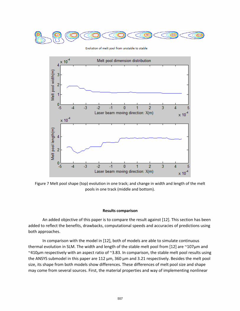
scanning center which is the horizontal axis in this model. Figure 7 is the evolution of the melt pool from

an unstable to a stable steady state. The melt pool shows asymmetry at several positions which are due

to the interaction with the previous track. This happens due to thermal accumulation with increasing

number of tracks. As soon as the laser beam turns back for a new track scan, the temperature close to

the point of track return is not able to cool down to the ambient temperature in the amount of time

available for it to do so. This forces a larger melt pool near turn locations and it reverses back to a stable

steady state after a short time. The bottom picture in figure 7 is the melt pool size history with the laser

beam movement in a particular track. Both the width and length of the melt pool approaches a stable

value. In addotopm, the width has faster convergence than the length.

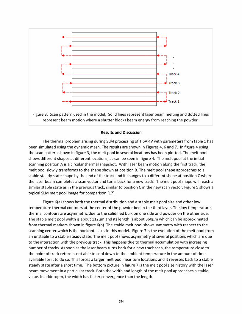
Figure 3. Scan pattern used in the model. Solid lines represent laser beam melting and dotted lines

represent beam motion where a shutter blocks beam energy from reaching the powder.

554

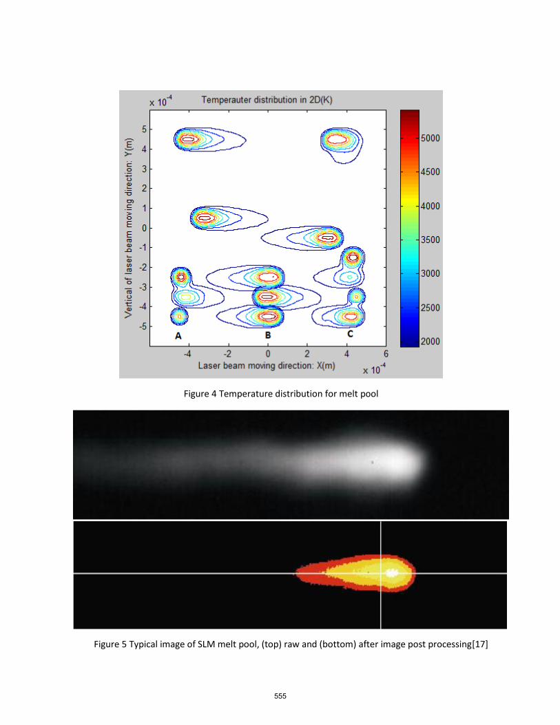
Figure 4 Temperature distribution for melt pool

Figure 5 Typical image of SLM melt pool, (top) raw and (bottom) after image post processing[17]

555

(a)

(b)

Figure 6 (a) Temperature distribution, (b) size of melt pool in stable

556

Results comparison

An added objective of this paper is to compare the result against [12]. This section has been

added to reflect the benefits, drawbacks, computational speeds and accuracies of predictions using

both approaches.

In comparison with the model in [12], both of models are able to simulate continuous

thermal evolution in SLM. The width and length of the stable melt pool from [12] are ~107µm and

~410µm respectively with an aspect ratio of ~3.83. In comparison, the stable melt pool results using

the ANSYS submodel in this paper are 112 µm, 360 µm and 3.21 respectively. Besides the melt pool

size, its shape from both models show differences. These differences of melt pool size and shape

may come from several sources. First, the material properties and way of implementing nonlinear

Figure 7 Melt pool shape (top) evolution in one track; and change in width and length of the melt

pools in one track (middle and bottom).

557

parameters may be different. The input of heat flux could also have effects since surface heat flux is

used in this paper rather than the volumetric heat flux in [12].

As discussed above, the model in this paper considers heat convection, phase change and

vaporization in the SLM process. It takes around 44 minutes to run the thermal picture for each

layer for the dimensions and mesh density shown in figure 2. It takes only 5 minutes for each layer

without considering the phase change and vaporization. The extra time for phase change and

vaporization is due to stricter convergence criteria when adding nonlinearities during the

calculation in ANSYS. The model is built in ANSYS 14.0 and the computer used to run the model is a

Dell Precision T1650 with 3.20GHz clock speed. A model with dimensions of 4x4x5mm runs for

about 11 hours for one layer of scanning simulation. For comparison, a model with similar

dimension and mesh density takes only 9 minutes using the further refined model employed in [12].

Therefore the approach described in [12] is ~66 times faster than a nearly identical dynamic model

run in ANSYS.

The SLM thermal problem is a highly specialized problem with extremely high energy input

in a tiny area, but which is applied recursively over a much larger part. Since ANSYS was not

designed specifically to solve this type of problem, it is not surprising that it takes much longer to

solve the model under consideration than the new approach developed in [12]. The success of the

ANSYS model is largely dependent on its advanced toolbox and it can serve as a useful method for

solving problems like SLM in the future.

Conclusions

Both ANSYS and the new finite element approach in [12] can simulate problems with spatio-

temporally periodic fluxes in small local area, such as the SLM process thermal problem. The model

in this paper overcomes the difficulty of building such problems in ANSYS. It provides a new way to

simulate SLM thermal problems for users trained in ANSYS. By comparison and contrast of the

model discussed in the paper against the model in [12] it is clear that although ANSYS can be used

to solve the SLM problem, other approaches have significant benefits for computational time and

efficiency.

Acknowledgement

The authors would like to acknowledge the Air Force Research Laboratory (AFRL) for support

through SBIR contract # FA8650-12-M-5153 provided to Mound Laser and Photonics Center (MLPC).

The formulations, modeling and validation activities involved in this work have been made possible

through a subcontract awarded to the University of Louisville (UL) by MLPC. The authors would like

to thank Dr. Larry Dosser, Mr. Kevin Hartke and Mr. Ron Jacobsen from MLPC and Mr. Tim Gornet

from Rapid Prototyping Center (RPC) at UL for access to experimental facilities during this work.

558

References

1. Gibson, I., D.W. Rosen, and B. Stucker, Additive manufacturing technologies: rapid prototyping to direct digital manufacturing. 2010: Springer.

2. Bremen, S., W. Meiners, and A. Diatlov, Selective Laser Melting. Laser Technik Journal, 2012. 9(2): p. 33-38.

3. Attar, E., Simulation of selective electron beam melting processes, 2011, Erlangen, Nurnberg, Univ., Diss., 2011.

4. Kruth, J.-P., et al., Selective laser melting of iron-based powder. Journal of Materials Processing Technology, 2004. 149(1): p. 616-622.

5. Zeng, K., D. Pal, and B. Stucker, A review of thermal analysis methods in Laser Sintering and Selective Laser Melting. Solid Freeform Fabrication Symposium, 2012(23): p. 796

6. Ibraheem, A.K., B. Derby, and P.J. Withers. Thermal and Residual Stress Modelling of the Selective Laser Sintering Process. in MATERIALS RESEARCH SOCIETY SYMPOSIUM PROCEEDINGS. 2003. Cambridge Univ Press.

7. Kolossov, S., et al., 3D FE simulation for temperature evolution in the selective laser sintering process. International Journal of Machine Tools and Manufacture, 2004. 44(2): p. 117-123.

8. Roberts, I., et al., A three-dimensional finite element analysis of the temperature field during laser melting of metal powders in additive layer manufacturing. International Journal of Machine Tools and Manufacture, 2009. 49(12): p. 916-923.

9. Song, B., et al., Process parameter selection for selective laser melting of Ti6Al4V based on temperature distribution simulation and experimental sintering. The International Journal of Advanced Manufacturing Technology, 2012. 61(9-12): p. 967-974.

10. Taylor, C.M., Direct laser sintering of stainless steel: thermal experiments and numerical modelling, 2004, The University of Leeds.

11. Zhang, D., et al., Select laser melting of W–Ni–Fe powders: simulation and experimental study. The International Journal of Advanced Manufacturing Technology, 2010. 51(5-8): p. 649-658.

12. Deepankar Pal , N.P., Khalid Rafia, Kai Zeng, Alleyce Moreland, Adam Hicks, David Beeler and Brent E. Stucker, A Feed Forward Dynamic Adaptive Mesh Refinement and De-refinement (FFD-AMRD) strategy for problems with non-linear spatiotemporally periodic localized boundary conditions Journal of applied physics, 2013.

13. Dowden, J.M., The mathematics of thermal modeling: an introduction to the theory of laser material processing. 2001: CRC Press.

14. Wang, X., et al., Direct selective laser sintering of hard metal powders: experimental study and simulation. The International Journal of Advanced Manufacturing Technology, 2002. 19(5): p. 351-357.

15. Li, J., L. Li, and F. Stott, Comparison of volumetric and surface heating sources in the modeling of laser melting of ceramic materials. International journal of heat and mass transfer, 2004. 47(6): p. 1159-1174.

16. Release, A., 12.0. ANSYS Theory Reference, 2009. 17. Kruth, J.-P., et al. Feedback control of selective laser melting. in Proceedings of the 3rd

International Conference on Advanced Research in Virtual and Rapid Prototyping. 2007.

559