Embed Size (px)
Citation preview

CENTRE NATIONAL DE LA RECHERCHESCIENTIFIQUE
A “New" Control Theory to Face the Challengesof Modern Technology
Romeo OrtegaLSS-Supelec, France
“A control theorist’s first instinct in the face of a new problem is to find a way to use the tools he
knows, rather that a commitment to understand the underlying phenomenon. This is not the failure of
individuals but the failure of our profession to foster the development of experimental control science.
In a way, we have become the prisoners of our rich inheritance and past successes”.
Y. C. Ho (1982).
Supelec, January 2012 – p. 1/91
CENTRE NATIONAL DE LA RECHERCHESCIENTIFIQUE
Layout
Introduction and Motivation
Control by Interconnection
Examples
Passivity–based Control
Mathematical Formulation
Applications
Mechanical systems
Power electronic systems
Electromechanical systems
Energy management
Transient stability of power systems
Wind speed estimation
Supelec, January 2012 – p. 2/91

CENTRE NATIONAL DE LA RECHERCHESCIENTIFIQUE
Introduction and Motivation
Supelec, January 2012 – p. 3/91

CENTRE NATIONAL DE LA RECHERCHESCIENTIFIQUE
Control Challenges in the Modern World
New engineering applications (including biomedical and others) exhibit:
Strong coupling between subsystems.
Mutually interacting, instead of cause–effect, relations.
Need for accurate, non–isolated, models.
Existing control theory, which adopts a signal–processing viewpoint, is inadequate toface those challenges.
Objective: Provide a new control paradigm, based on considerations of
energy,
dissipation and
interconnection.
Paradigmatic examples
Modern electrical (smart) grid
Interacting mechanical systems, e.g. teleoperators, cooperative robots...
Transportation systems
Bio–medical applications...
Supelec, January 2012 – p. 4/91
CENTRE NATIONAL DE LA RECHERCHESCIENTIFIQUE
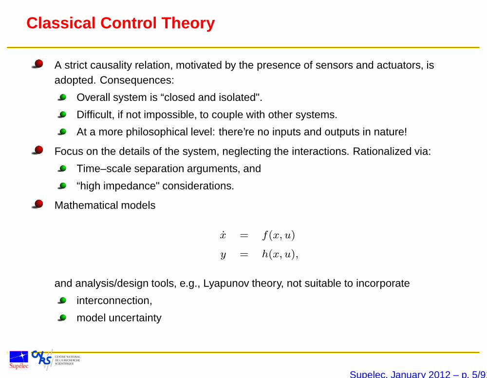
Classical Control Theory
A strict causality relation, motivated by the presence of sensors and actuators, isadopted. Consequences:
Overall system is “closed and isolated".
Difficult, if not impossible, to couple with other systems.
At a more philosophical level: there’re no inputs and outputs in nature!
Focus on the details of the system, neglecting the interactions. Rationalized via:
Time–scale separation arguments, and
“high impedance" considerations.
Mathematical models
x = f(x, u)
y = h(x, u),
and analysis/design tools, e.g., Lyapunov theory, not suitable to incorporate
interconnection,
model uncertainty
Supelec, January 2012 – p. 5/91
CENTRE NATIONAL DE LA RECHERCHESCIENTIFIQUE
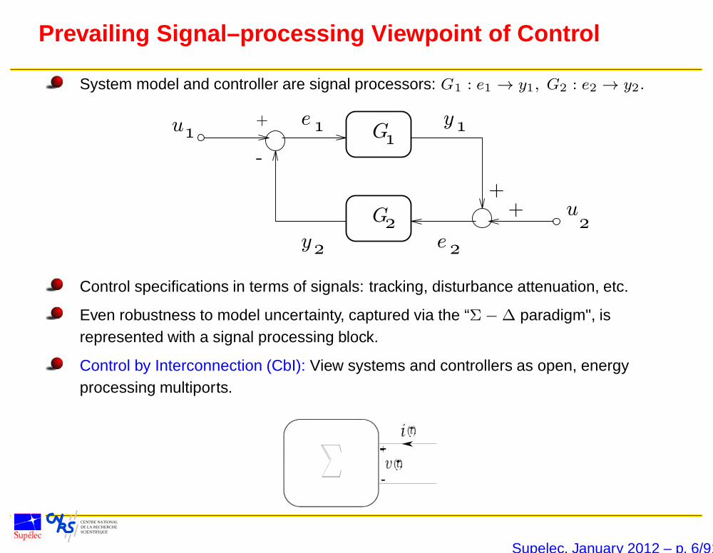
Prevailing Signal–processing Viewpoint of Control
System model and controller are signal processors: G1 : e1 → y1, G2 : e2 → y2.
1
2
+
+
-
+u y
u
y
1
2
1e
e 2
G
G2
1
Control specifications in terms of signals: tracking, disturbance attenuation, etc.
Even robustness to model uncertainty, captured via the “Σ−∆ paradigm", isrepresented with a signal processing block.
Control by Interconnection (CbI): View systems and controllers as open, energyprocessing multiports.
Supelec, January 2012 – p. 6/91

CENTRE NATIONAL DE LA RECHERCHESCIENTIFIQUE
Control by Interconnection
Supelec, January 2012 – p. 7/91
CENTRE NATIONAL DE LA RECHERCHESCIENTIFIQUE
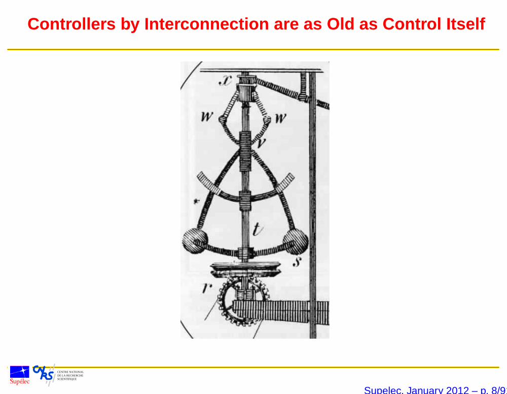
Controllers by Interconnection are as Old as Control Itself
Supelec, January 2012 – p. 8/91
CENTRE NATIONAL DE LA RECHERCHESCIENTIFIQUE
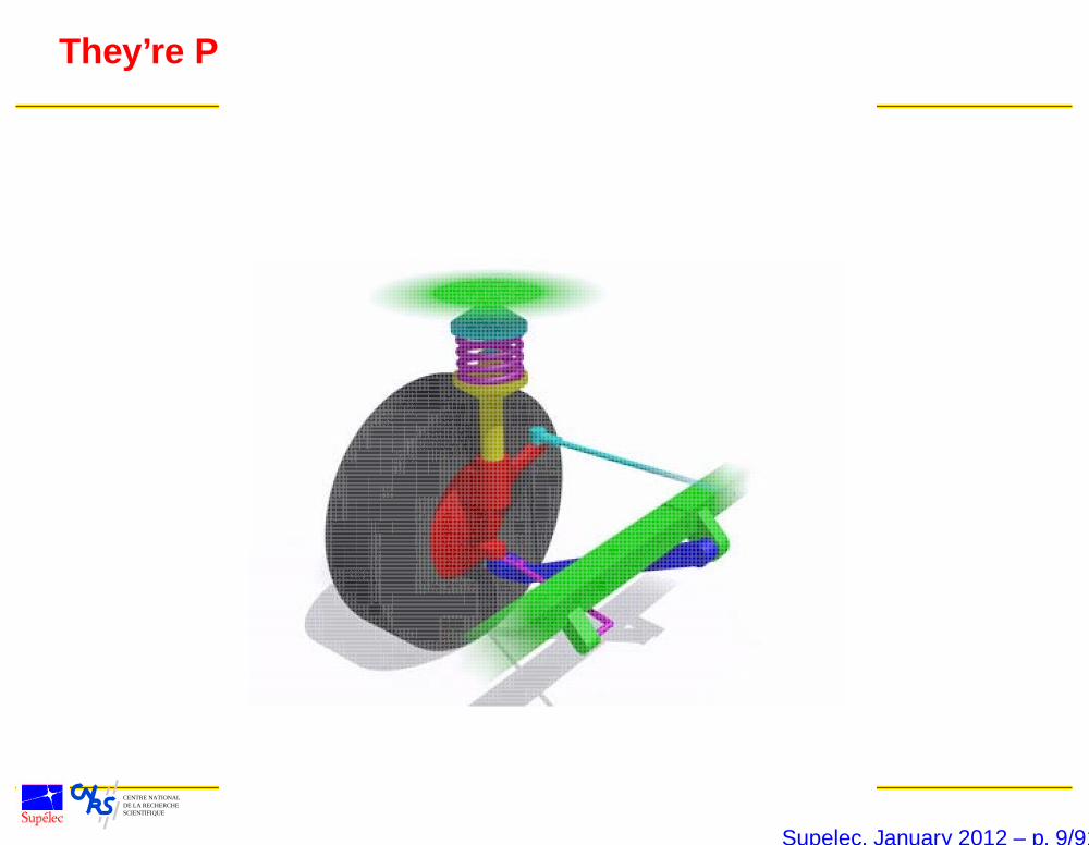
They’re Pervasive and Efficient
Supelec, January 2012 – p. 9/91

CENTRE NATIONAL DE LA RECHERCHESCIENTIFIQUE
Even in your Privy
Supelec, January 2012 – p. 10/91

CENTRE NATIONAL DE LA RECHERCHESCIENTIFIQUE
Interconnection Works Even if We Don’t Know Why!
(Spong’06): Synchronization by interconnection, an openproblem since the 17th century.♥
Supelec, January 2012 – p. 11/91
CENTRE NATIONAL DE LA RECHERCHESCIENTIFIQUE
Passivity: The Key Articulating Concept
Why is passivity important?
For physical systems it is a restatement of energy conservation.
Is a natural generalization (to NL dynamical systems) of positivity of matrices andphase-shift of LTI systems—sign preserving property.
Term Passivity–based Control (PBC) introduced in
R. Ortega and M. Spong, Adaptive Motion Control Of Rigid Robots: A Tutorial,Automatica, Vol. 25, No. 6, 1989, pp. 877-888,
to define a controller methodology whose aim is to render the closed–loop passive.
It was done in the context of adaptive control of robot manipulators.
Natural, because mechanical systems and parameter estimators define passive maps.
The paper
has been cited more than 900 times and
is the 13th most highly cited paper out of 4520 published in Automatica since1989.
PBC has more than 100,000 hits in Google scholar.
Supelec, January 2012 – p. 12/91

CENTRE NATIONAL DE LA RECHERCHESCIENTIFIQUE
Passivity–Based Control: An Energy–Processing Viewpoint
View plant as energy–transformation multiport devices
Physical systems satisfy (generalized) energy–conservation:
Stored energy = Supplied energy + Dissipation
Control objective in PBC: preserve the energy–conservation property but with desiredenergy and dissipation functions
Desired stored energy = New supplied energy + Desired dissipation
In other words
PBC = Energy Shaping + Damping Assignment
For general systems achieve a passivation objective
Three possible formulations.
State feedback either to passivize or to change the energy function (anddissipation).
Control by Interconnection (CbI)—plant and controller are energy–transformationdevices, whose energy is added up.
Decompose the system into passive (or passifiable) sub-blocks and design PBCsfor each one of them.
Supelec, January 2012 – p. 13/91

CENTRE NATIONAL DE LA RECHERCHESCIENTIFIQUE
Passivity as a Design Tool: Foundational Results
(Moylan and Anderson, TAC’73): Optimal systems define passive maps. Nonlinearextension of Kalman’s inverse optimal control result.
(Fradkov, Aut and Rem Control’76): Necessary and sufficient conditions for passivationof LTI systems via state feedback.
(Takegaki and Arimoto, ASME JDSM&C’81), (Jonckheere, European Conf Circ. Th.and Design’81): Potential energy shaping and damping injection as design tools formechanical and electromechanical systems—new energy function as Lyapunovfunction.
(Kokotovic and Sussmann, S&CL’89): Stabilization of a NL system in cascade with anintegrator using positive realness.
(Ortega, Automatica’91): Extension to cascade of two NL systems using Hill/Moylantheorem.
(Byrnes, Isidori and Willems, TAC’91): Complete geometric characterization ofpassifiable systems—via minimum phase and relative degree conditions.
Backstepping and forwarding are passivation recursive designs that overcome theobstacles of relative degree and minimum phase for systems with special structures.See e.g., (Astolfi, Ortega and Sepulchre, EJC’02).
Supelec, January 2012 – p. 14/91

CENTRE NATIONAL DE LA RECHERCHESCIENTIFIQUE
Advantages of PBC
Energy and dissipation are additive.
Applicable to NL systems.
Suitable to handle interconnections of open systems.
Model uncertainty, e.g., friction, naturally captured.
Shaping energy and dissipation there’s a handle on performance, not just stability
Respect, and effectively exploit, the structure of the system to
incorporate physical knowledge,
provide physical interpretations to the control action.
Energy conservation is a universal property, hence CbI is applicable to multi–domainphysical systems.
Energy serves as a lingua franca to communicate with practitioners.
There’s an elegant geometrical characterization of
power–conserving interconnections (via Dirac structures) and
passifiable NL systems (in terms of stable invertibility and relative degree)
Supelec, January 2012 – p. 15/91
CENTRE NATIONAL DE LA RECHERCHESCIENTIFIQUE
Applications
Mechanical systems: walking robots, bilateral teleoperators, pendular systems.
Chemical processes: mass–balance systems, inventory control, reactors.
Electrical systems: power systems, power converters.
Electromechanical systems: motors, magnetic levitation systems, windmill generators.
Transportation systems: underwater vehicles, surface vessels, (air)spacecrafts.
Control over networks: formation control, synchronization, consensus problems.
Hybrid systems: switched systems, hybrid passivity.
...
Supelec, January 2012 – p. 16/91

CENTRE NATIONAL DE LA RECHERCHESCIENTIFIQUE
Mathematical Formulation of CbI
Supelec, January 2012 – p. 17/91
CENTRE NATIONAL DE LA RECHERCHESCIENTIFIQUE
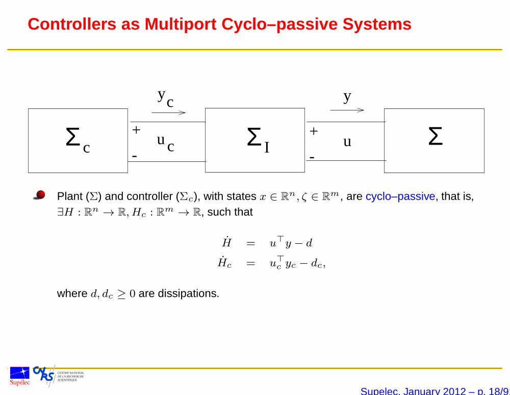
Controllers as Multiport Cyclo–passive Systems
cΣ-
+
-
+ Σu c
yc y
uΣ I
Plant (Σ) and controller (Σc), with states x ∈ Rn, ζ ∈ R
m, are cyclo–passive, that is,∃H : Rn → R, Hc : Rm → R, such that
H = u>y − d
Hc = u>c yc − dc,
where d, dc ≥ 0 are dissipations.
Supelec, January 2012 – p. 18/91
CENTRE NATIONAL DE LA RECHERCHESCIENTIFIQUE
Adding the Energies
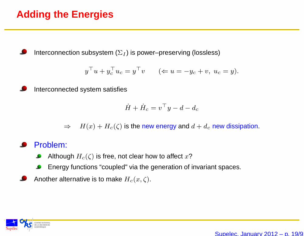
Interconnection subsystem (ΣI ) is power–preserving (lossless)
y>u+ y>c uc = y>v (⇐ u = −yc + v, uc = y).
Interconnected system satisfies
H + Hc = v>y − d− dc
⇒ H(x) +Hc(ζ) is the new energy and d+ dc new dissipation.
Problem:Although Hc(ζ) is free, not clear how to affect x?
Energy functions “coupled" via the generation of invariant spaces.
Another alternative is to make Hc(x, ζ).
Supelec, January 2012 – p. 19/91
CENTRE NATIONAL DE LA RECHERCHESCIENTIFIQUE
Invariant Function Method
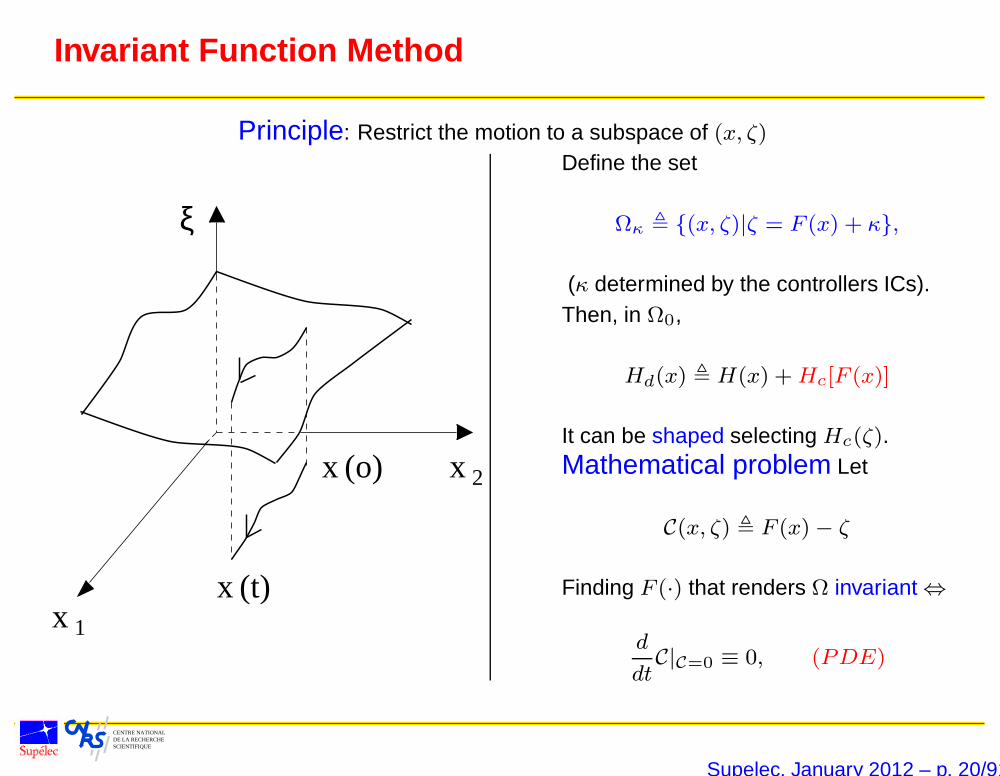
Principle: Restrict the motion to a subspace of (x, ζ)
1
x (t)
x (o) x
x
2
ξ
Define the set
Ωκ , (x, ζ)|ζ = F (x) + κ,
(κ determined by the controllers ICs).Then, in Ω0,
Hd(x) , H(x) +Hc[F (x)]
It can be shaped selecting Hc(ζ).Mathematical problem Let
C(x, ζ) , F (x)− ζ
Finding F (·) that renders Ω invariant ⇔
d
dtC|C=0 ≡ 0, (PDE)
Supelec, January 2012 – p. 20/91
CENTRE NATIONAL DE LA RECHERCHESCIENTIFIQUE
Suitable Model: Port–Hamiltonian Systems
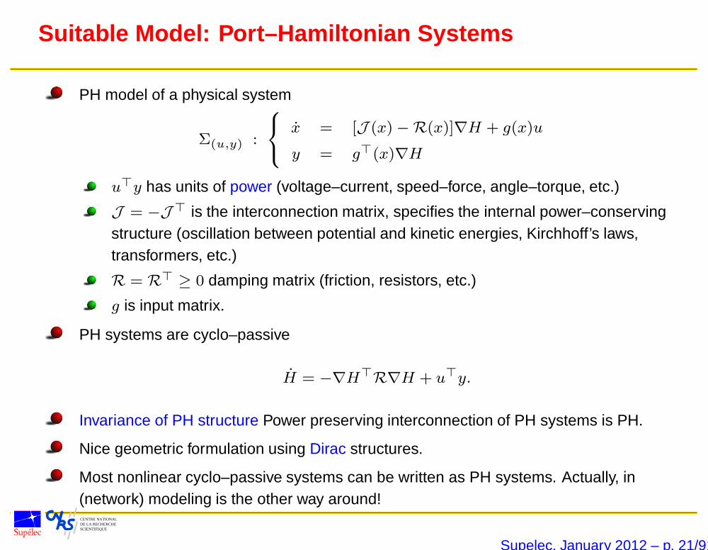
PH model of a physical system
Σ(u,y) :
x = [J (x)−R(x)]∇H + g(x)u
y = g>(x)∇H
u>y has units of power (voltage–current, speed–force, angle–torque, etc.)
J = −J> is the interconnection matrix, specifies the internal power–conservingstructure (oscillation between potential and kinetic energies, Kirchhoff’s laws,transformers, etc.)
R = R> ≥ 0 damping matrix (friction, resistors, etc.)
g is input matrix.
PH systems are cyclo–passive
H = −∇H>R∇H + u>y.
Invariance of PH structure Power preserving interconnection of PH systems is PH.
Nice geometric formulation using Dirac structures.
Most nonlinear cyclo–passive systems can be written as PH systems. Actually, in(network) modeling is the other way around!
Supelec, January 2012 – p. 21/91
CENTRE NATIONAL DE LA RECHERCHESCIENTIFIQUE
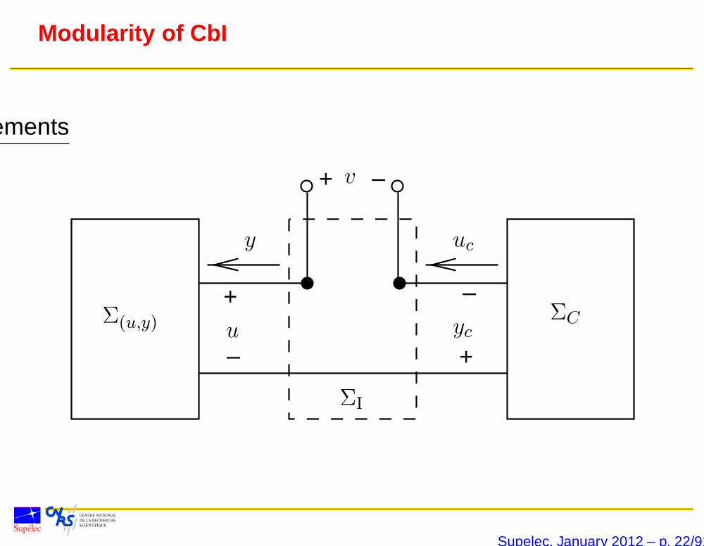
Modularity of CbI
PSfrag replacements
+
+
+
–
–
–
v
Σ(u,y) ΣC
ΣI
y
ycu
uc
Supelec, January 2012 – p. 22/91

CENTRE NATIONAL DE LA RECHERCHESCIENTIFIQUE
Mechanical Systems
Supelec, January 2012 – p. 23/91
CENTRE NATIONAL DE LA RECHERCHESCIENTIFIQUE
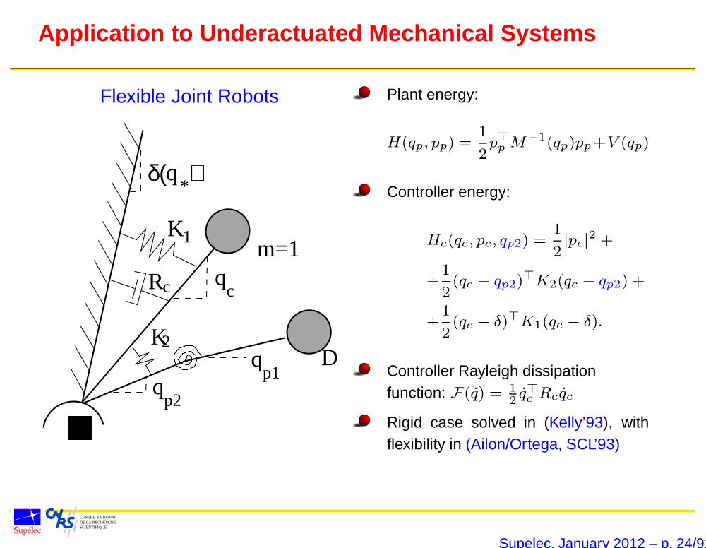
Application to Underactuated Mechanical Systems
Flexible Joint Robots
q c
q *
δ( )
q q
p1
p2
K 2
Rc
K 1m=1
D
Plant energy:
H(qp, pp) =1
2p>p M
−1(qp)pp+V (qp)
Controller energy:
Hc(qc, pc, qp2) =1
2|pc|
2 +
+1
2(qc − qp2)
>K2(qc − qp2) +
+1
2(qc − δ)>K1(qc − δ).
Controller Rayleigh dissipationfunction: F(q) = 1
2q>c Rcqc
Rigid case solved in (Kelly’93), withflexibility in (Ailon/Ortega, SCL’93)
Supelec, January 2012 – p. 24/91
CENTRE NATIONAL DE LA RECHERCHESCIENTIFIQUE
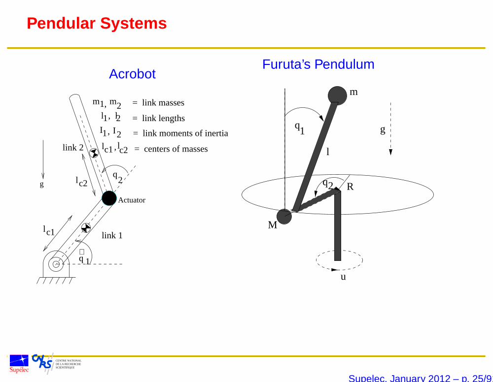
Pendular Systems
Acrobot
g
Actuator
l
l
c1
c2
link 2
link 1
q2
m m1, 2l , l1 2I I, 21
lc1 , lc2
= link masses
= link lengths
= link moments of inertia
= centers of masses
1q∼
Furuta’s Pendulum
q1
m
l
2q R
M
u
g
Supelec, January 2012 – p. 25/91
CENTRE NATIONAL DE LA RECHERCHESCIENTIFIQUE
Performance Improvement via Energy Shaping
Transient Performance of the Ball and Beam
Steep energy function ⇒ quick response but bad transient ♥
“Wider" energy function ⇒ slower response without overshoot transient ♥
No regulation of transient excursions ⇒ ball gets off the bar ♥
Limiting level sets ⇒ ball remains in the bar ♥
Smooth Swing–up of Underactuated Mechanical Systems
Acrobot ♥ In (Viola, et al.’08) first proof of stability including the lower half plane.
Furuta’s Pendulum ♥
Orbital Stabilization of Passive Walking Robot
Problem cannot be posed in terms of tracking, a natural approach is to regulatethe kinetic–potential energy exchange ♥
‘Achieved assigning an energy function like a "Mexican sombrero" ♥
Supelec, January 2012 – p. 26/91
CENTRE NATIONAL DE LA RECHERCHESCIENTIFIQUE
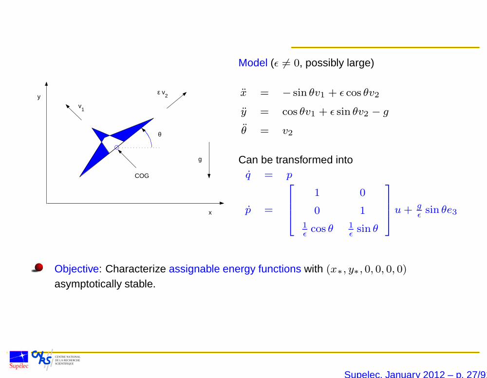
Strongly Coupled VTOL Aircraft
θ
x
y ε v
2
v1
g
COG
Model (ε 6= 0, possibly large)
x = − sin θv1 + ε cos θv2
y = cos θv1 + ε sin θv2 − g
θ = v2
Can be transformed intoq = p
p =
1 0
0 1
1εcos θ 1
εsin θ
u+ g
εsin θe3
Objective: Characterize assignable energy functions with (x∗, y∗, 0, 0, 0, 0)
asymptotically stable.
Supelec, January 2012 – p. 27/91
CENTRE NATIONAL DE LA RECHERCHESCIENTIFIQUE
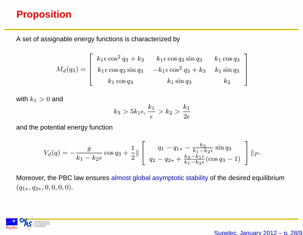
Proposition
A set of assignable energy functions is characterized by
Md(q3) =
k1ε cos2 q3 + k3 k1ε cos q3 sin q3 k1 cos q3
k1ε cos q3 sin q3 −k1ε cos2 q3 + k3 k1 sin q3
k1 cos q3 k1 sin q3 k2
with k1 > 0 and
k3 > 5k1ε,k1
ε> k2 >
k1
2ε
and the potential energy function
Vd(q) = −g
k1 − k2εcos q3 +
1
2‖
q1 − q1∗ − k3
k1−k2εsin q3
q2 − q2∗ + k3−k1εk1−k2ε
(cos q3 − 1)
‖P .
Moreover, the PBC law ensures almost global asymptotic stability of the desired equilibrium(q1∗, q2∗, 0, 0, 0, 0).
Supelec, January 2012 – p. 28/91
CENTRE NATIONAL DE LA RECHERCHESCIENTIFIQUE
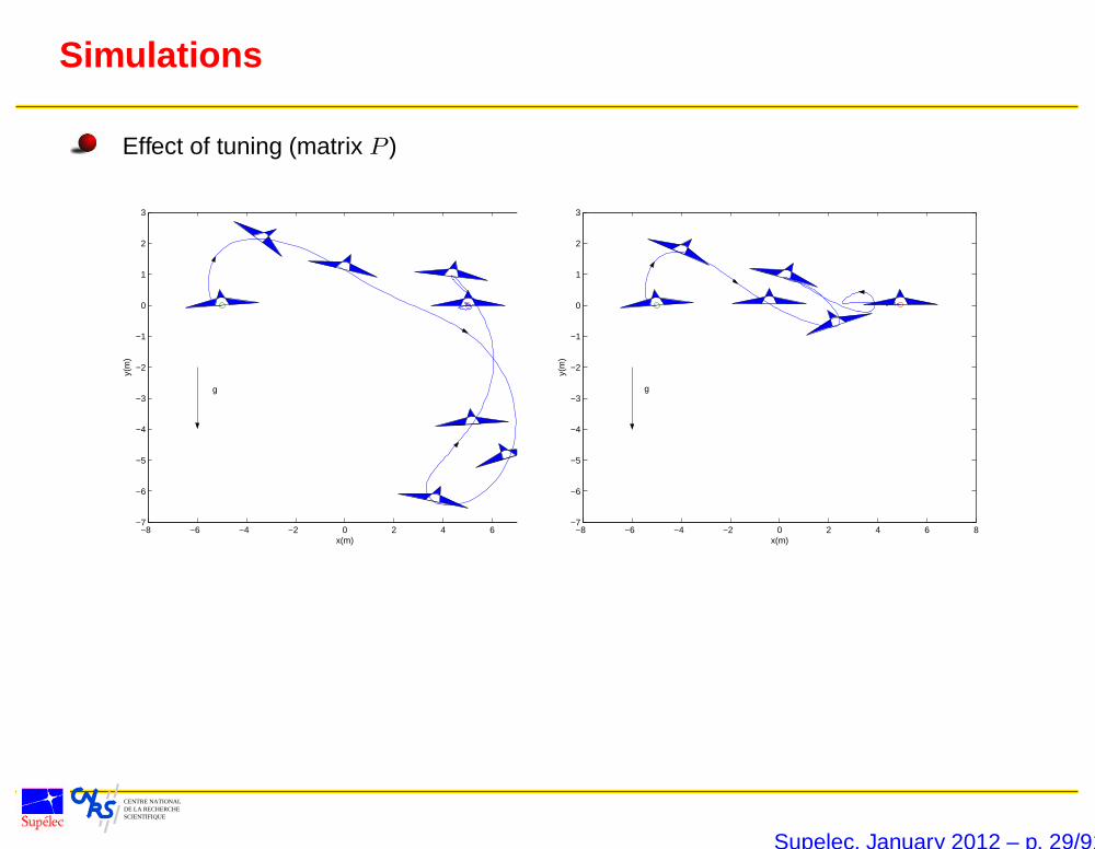
Simulations
Effect of tuning (matrix P )
−8 −6 −4 −2 0 2 4 6 8−7
−6
−5
−4
−3
−2
−1
0
1
2
3
x(m)
y(m
)
g
−8 −6 −4 −2 0 2 4 6 8−7
−6
−5
−4
−3
−2
−1
0
1
2
3
x(m)
y(m
)
g
Supelec, January 2012 – p. 29/91
CENTRE NATIONAL DE LA RECHERCHESCIENTIFIQUE
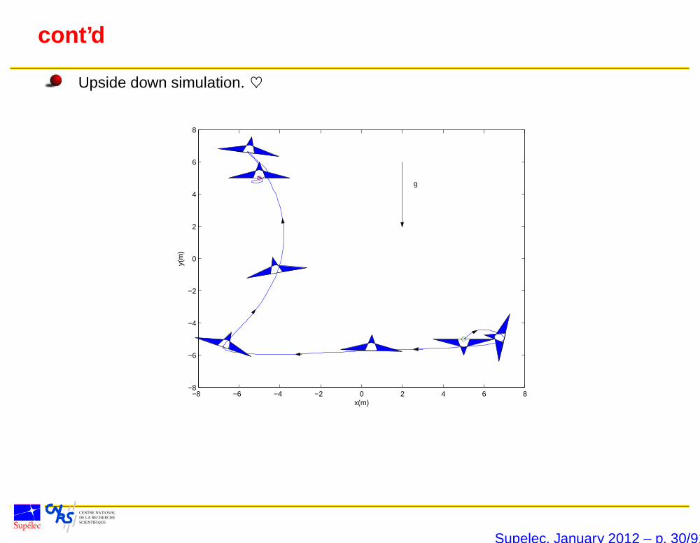
cont’d
Upside down simulation. ♥
−8 −6 −4 −2 0 2 4 6 8−8
−6
−4
−2
0
2
4
6
8
x(m)
y(m
)g
Supelec, January 2012 – p. 30/91
CENTRE NATIONAL DE LA RECHERCHESCIENTIFIQUE
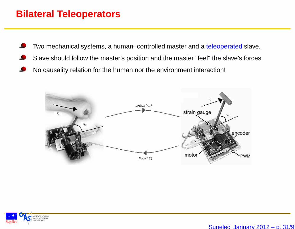
Bilateral Teleoperators
Two mechanical systems, a human–controlled master and a teleoperated slave.
Slave should follow the master’s position and the master “feel" the slave’s forces.
No causality relation for the human nor the environment interaction!
Supelec, January 2012 – p. 31/91
CENTRE NATIONAL DE LA RECHERCHESCIENTIFIQUE
cont’d
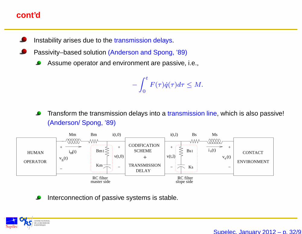
Instability arises due to the transmission delays.
Passivity–based solution (Anderson and Spong, ’89)
Assume operator and environment are passive, i.e.,
−
∫ t
0F (τ)q(τ)dτ ≤M.
Transform the transmission delays into a transmission line, which is also passive!(Anderson/ Spong, ’89)
TRANSMISSION DELAY
CODIFICATION SCHEME
ENVIRONMENT
CONTACT
RC filtermaster side
RC filterslope side
i(t,0)
v(t,0)
Bs
Km
Bm
Mm Bm Ms
Bs
Ks
i(t,l)
+
−
+ +
− −
+
−
h e
s
OPERATOR
HUMAN+
1 1mi (t)i (t)
v(t,l)v (t) v (t)
Interconnection of passive systems is stable.
Supelec, January 2012 – p. 32/91
CENTRE NATIONAL DE LA RECHERCHESCIENTIFIQUE
A Dual Problem
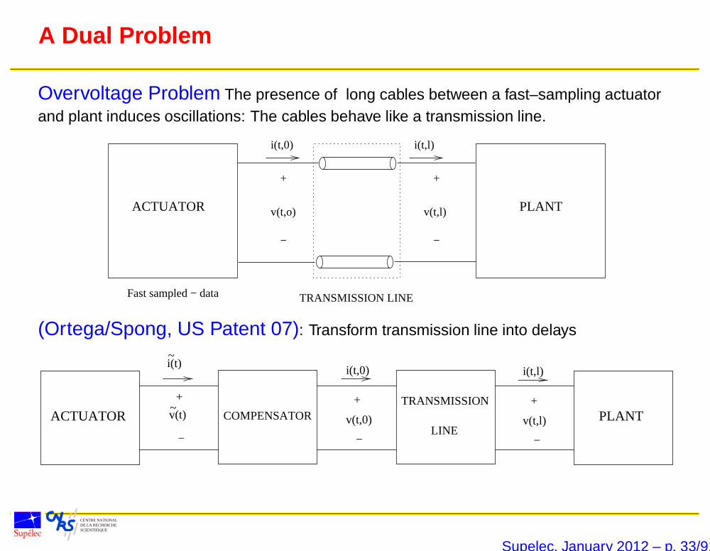
Overvoltage Problem The presence of long cables between a fast–sampling actuatorand plant induces oscillations: The cables behave like a transmission line.
v(t,l)v(t,o)
i(t,0) i(t,l)
+ +
− −
ACTUATOR
TRANSMISSION LINEFast sampled − data
PLANT
(Ortega/Spong, US Patent 07): Transform transmission line into delays
ACTUATOR PLANTCOMPENSATORTRANSMISSION
LINE
+
−
i(t,l)
v(t,l)
−
+
i(t,0)
v(t,0)
−
+
i(t)
v(t)~
~
Supelec, January 2012 – p. 33/91
CENTRE NATIONAL DE LA RECHERCHESCIENTIFIQUE
Synchronization of Uncertain Euler–Lagrange Systems
N Euler–Lagrange systems described by
Mi(qi)qi + Ci(qi, qi)qi + gi(qi) = τi,
where all parameters are unknown.
Interconnected through a communication channel
With unknown transmission delays.
Only weakly connected.
Objective: Find a dynamics controller that achieves either
synchronization, that is, qi(t) → qd(t), or
consensus, qi(t)− qj(t) → 0.
Reported in (Nuño, et al.’10)
Experiments between the UdG (Guadalajara) and UPCatalonya (Barcelona)interconnected via Internet
Three coordinated Phantoms ♥
Teleoperation between Guadalajara and Barcelona ♥
Supelec, January 2012 – p. 34/91

CENTRE NATIONAL DE LA RECHERCHESCIENTIFIQUE
Electrical Systems
Supelec, January 2012 – p. 35/91

CENTRE NATIONAL DE LA RECHERCHESCIENTIFIQUE
PI Control of Power Converters
Supelec, January 2012 – p. 36/91
CENTRE NATIONAL DE LA RECHERCHESCIENTIFIQUE
Problem Formulation
A large class of power converters are modeled by
x =
(J0 +
m∑
i=1
Jiui − R
)∇H(x) +
(G0 +
m∑
i=1
Giui
)E (SW )
where x ∈ Rn is the converter state (typically containing inductor fluxes and capacitor
charges), u ∈ Rm denotes the duty ratio of the switches, the total energy stored in
inductors and capacitors is
H(x) = 12x>Qx , Q = Q> > 0
Ji = −J>i i ∈ m := 0, . . . ,m are the interconnection matrices, R = R> ≥ 0
represents the dissipation matrix, and the vector Gi ∈ Rn contains the (possibly
switched) external voltage and current sources.
The control objective is to stabilize and equilibrium x? ∈ Rn.
It is desirable to propose simple, robust controllers.
(Hernandez, et al., IEEE TCST’10; ISIE’10)
Supelec, January 2012 – p. 37/91
CENTRE NATIONAL DE LA RECHERCHESCIENTIFIQUE
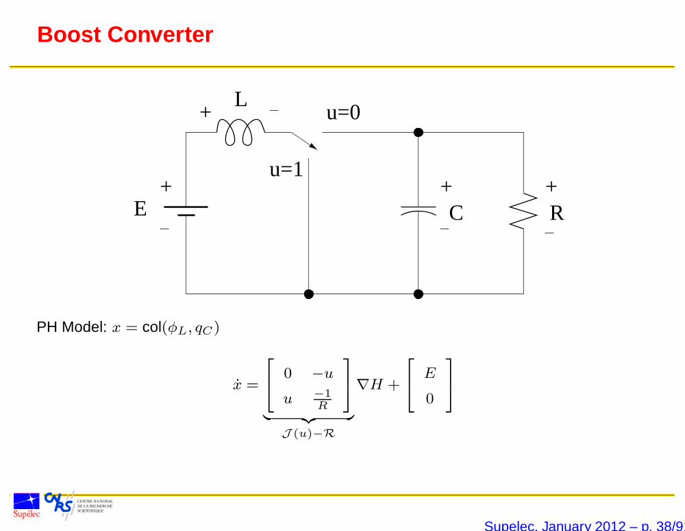
Boost Converter
+
L+
+E
u=0
u=1
C+
R
PH Model: x = col(φL, qC)
x =
0 −u
u −1R
︸ ︷︷ ︸J (u)−R
∇H +
E
0
Supelec, January 2012 – p. 38/91
CENTRE NATIONAL DE LA RECHERCHESCIENTIFIQUE
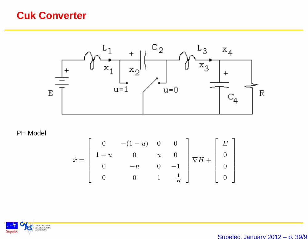
Cuk Converter
PH Model
x =
0 −(1− u) 0 0
1− u 0 u 0
0 −u 0 −1
0 0 1 − 1R
∇H +
E
0
0
0
Supelec, January 2012 – p. 39/91

CENTRE NATIONAL DE LA RECHERCHESCIENTIFIQUE
An Incremental Passivity Property
Let x∗ ∈ Rn be an admissible equilibrium point, that is, x∗ satisfies
0 =
(J0 +
m∑
i=1
Jiu∗i − R
)∇H(x∗) +
(G0 +
m∑
i=1
Giu∗i
)E,
for some u∗ ∈ Rm. The incremental model of the system for the output y = Cx, where
C :=
E>G>1 − (x∗)>QJ1
...
E>G>m − (x∗)>QJm
Q ∈ R
m×n,
is passive. More precisely, the system verifies the dissipation inequality V ≤ y>u, wherey∗ = Cx∗ and the (positive definite) storage function is given by
V (x) :=1
2(x− x∗)>Q(x− x∗).
Supelec, January 2012 – p. 40/91
CENTRE NATIONAL DE LA RECHERCHESCIENTIFIQUE
Corollary: Global Asymptotic Stabilization with a PI
Consider a switched power converter described by (SW) in closed loop with the PI controller
z = −y
u = −Kpy +Kiz,
where Kp,Ki ∈ Rm×m are symmetric positive definite matrices, y = Cx. For all initial
conditions (x(0), z(0)) ∈ Rn+m the trajectories of the closed–loop system are bounded and
such that
limt→∞
Cx(t) = 0.
Moreover,
limt→∞
x(t) = x∗,
if y is detectable, that is, if for any solution x(t) of the system the following implication is true:
Cx(t) ≡ Cx∗ ⇒ limt→∞
x(t) = x∗.
Supelec, January 2012 – p. 41/91
CENTRE NATIONAL DE LA RECHERCHESCIENTIFIQUE
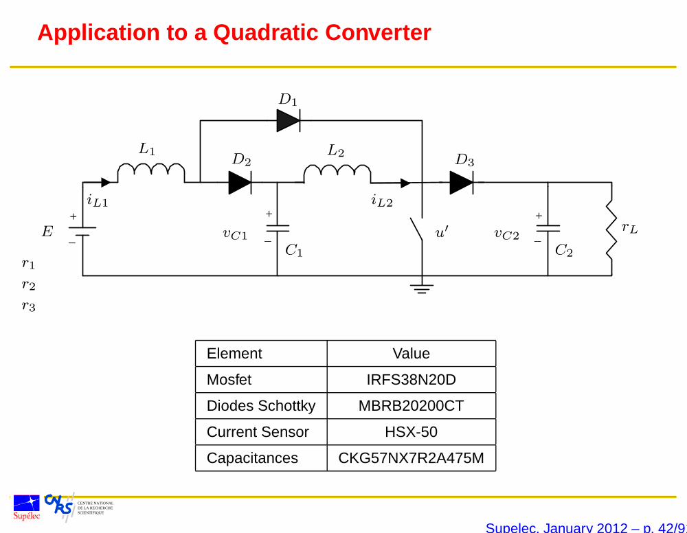
Application to a Quadratic Converter
+
_
+
_
+
_
PSfrag replacements
E
L1 L2
C1 C2
D1
D2 D3
iL1 iL2
vC1 vC2rLu′
r1
r2
r3
Element Value
Mosfet IRFS38N20D
Diodes Schottky MBRB20200CT
Current Sensor HSX-50
Capacitances CKG57NX7R2A475M
Supelec, January 2012 – p. 42/91
CENTRE NATIONAL DE LA RECHERCHESCIENTIFIQUE
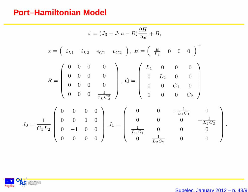
Port–Hamiltonian Model
x = (J0 + J1u−R)∂H
∂x+ B,
x =(iL1 iL2 vC1 vC2
), B =
(EL1
0 0 0)>
R =
0 0 0 0
0 0 0 0
0 0 0 0
0 0 0 1rLC2
2
, Q =
L1 0 0 0
0 L2 0 0
0 0 C1 0
0 0 0 C2
J0 =1
C1L2
0 0 0 0
0 0 1 0
0 −1 0 0
0 0 0 0
J1 =
0 0 − 1L1C1
0
0 0 0 − 1L2C2
1L1C1
0 0 0
0 1L2C2
0 0
.
Supelec, January 2012 – p. 43/91
CENTRE NATIONAL DE LA RECHERCHESCIENTIFIQUE
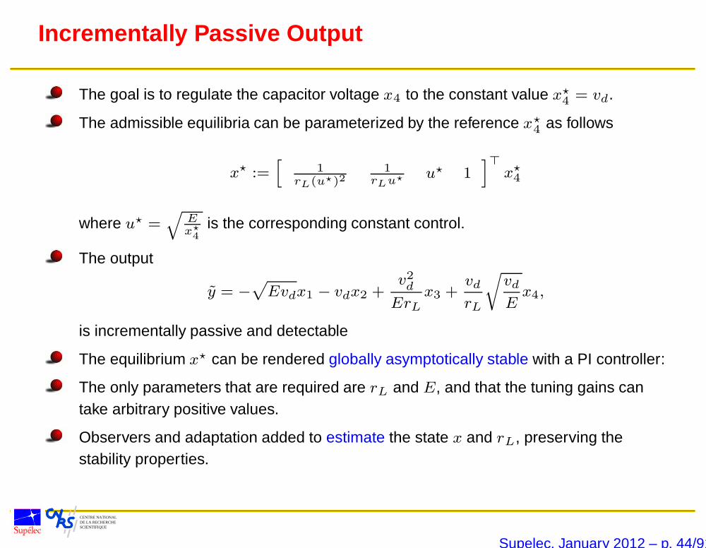
Incrementally Passive Output
The goal is to regulate the capacitor voltage x4 to the constant value x?4 = vd.
The admissible equilibria can be parameterized by the reference x?4 as follows
x? :=[
1rL(u?)2
1rLu? u? 1
]>x?4
where u? =√
Ex?4
is the corresponding constant control.
The output
y = −√Evdx1 − vdx2 +
v2dErL
x3 +vd
rL
√vd
Ex4,
is incrementally passive and detectable
The equilibrium x? can be rendered globally asymptotically stable with a PI controller:
The only parameters that are required are rL and E, and that the tuning gains cantake arbitrary positive values.
Observers and adaptation added to estimate the state x and rL, preserving thestability properties.
Supelec, January 2012 – p. 44/91
CENTRE NATIONAL DE LA RECHERCHESCIENTIFIQUE
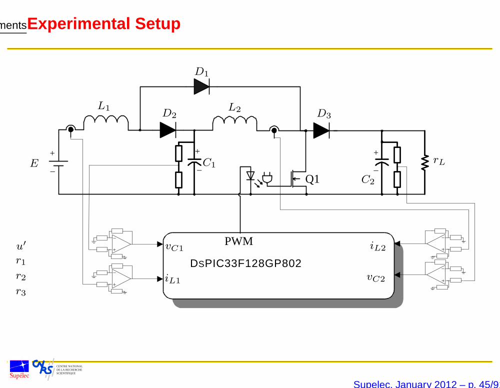
Experimental Setup
Q1
+
_
+
_
+
_
PWM
PSfrag replacements
E
L1 L2
C1
C2
D1
D2 D3
iL1
iL2vC1
vC2
rL
u′
r1
r2
r3
DSPIC33F128GP802
Supelec, January 2012 – p. 45/91
CENTRE NATIONAL DE LA RECHERCHESCIENTIFIQUE
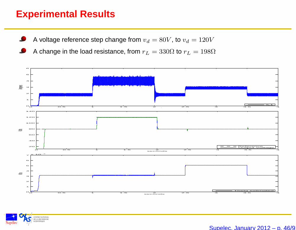
Experimental Results
A voltage reference step change from vd = 80V , to vd = 120V
A change in the load resistance, from rL = 330Ω to rL = 198Ω
0 0.5 1 1.5 2 2.5 3 3.5 40
1
2
3
4
5
6
Amperes
seconds
iL1
0 0.5 1 1.5 2 2.5 3 3.5 4
20
40
60
80
100
120
140
Volts
seconds
ReferenceOutput Voltage
0 0.5 1 1.5 2 2.5 3 3.5 40
1
2
3
4
5
6
7x 10
−3
Mho
seconds
Theta estimated
Supelec, January 2012 – p. 46/91
CENTRE NATIONAL DE LA RECHERCHESCIENTIFIQUE
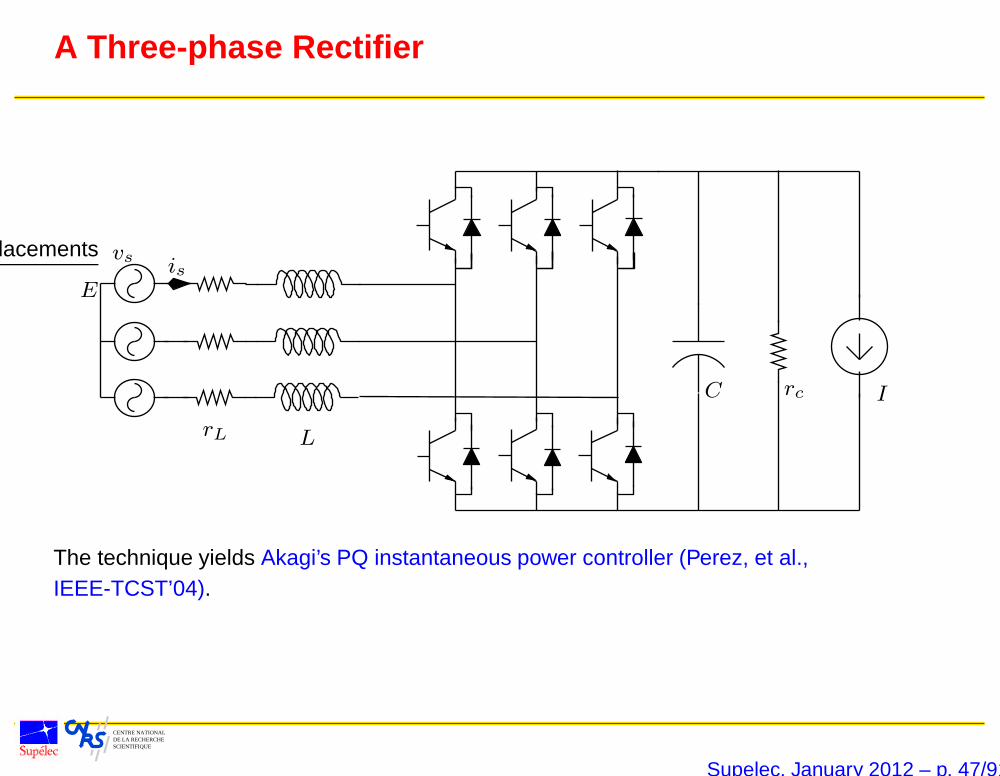
A Three-phase Rectifier
PSfrag replacements
E
vs
rL L
IC rc
is
The technique yields Akagi’s PQ instantaneous power controller (Perez, et al.,IEEE-TCST’04).
Supelec, January 2012 – p. 47/91

CENTRE NATIONAL DE LA RECHERCHESCIENTIFIQUE
Some Additional Results
An adaptive observer–based PBC for the SEPIC, (Jaafar, et al., ACC’12).
Control of converters in discontinuous conduction mode, (Allawieh, et al., IFAC’11).
An adaptive PBC for a unity power factor rectifier, (Escobar, et al., IEEE TCST’01).
Experimental comparison of several PWM controllers for a single-phase ac-dcconverter, (Karagiannis, et al., IEEE-TCST’03).
An adaptive controller for the shunt active filter considering a dynamic load and the lineimpedance, (Valdez, et al., IEEE-TCST’09).
Supelec, January 2012 – p. 48/91

CENTRE NATIONAL DE LA RECHERCHESCIENTIFIQUE
Transient Stability of Power Systems
Supelec, January 2012 – p. 49/91
CENTRE NATIONAL DE LA RECHERCHESCIENTIFIQUE
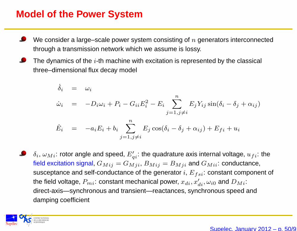
Model of the Power System
We consider a large–scale power system consisting of n generators interconnectedthrough a transmission network which we assume is lossy.
The dynamics of the i-th machine with excitation is represented by the classicalthree–dimensional flux decay model
δi = ωi
ωi = −Diωi + Pi −GiiE2i −Ei
n∑
j=1,j 6=i
EjYij sin(δi − δj + αij)
Ei = −aiEi + bi
n∑
j=1,j 6=i
Ej cos(δi − δj + αij) +Efi + ui
δi, ωMi: rotor angle and speed, E′qi: the quadrature axis internal voltage, ufi: the
field excitation signal, GMij = GMji, BMij = BMji and GMii: conductance,susceptance and self-conductance of the generator i, Efsi: constant component ofthe field voltage, Pmi: constant mechanical power, xdi, x′di, ωi0 and DMi:direct-axis—synchronous and transient—reactances, synchronous speed anddamping coefficient
Supelec, January 2012 – p. 50/91
CENTRE NATIONAL DE LA RECHERCHESCIENTIFIQUE
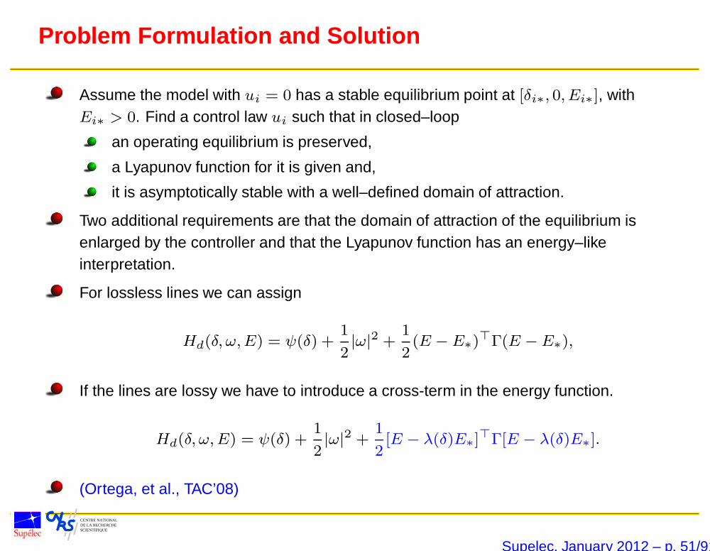
Problem Formulation and Solution
Assume the model with ui = 0 has a stable equilibrium point at [δi∗, 0, Ei∗], withEi∗ > 0. Find a control law ui such that in closed–loop
an operating equilibrium is preserved,
a Lyapunov function for it is given and,
it is asymptotically stable with a well–defined domain of attraction.
Two additional requirements are that the domain of attraction of the equilibrium isenlarged by the controller and that the Lyapunov function has an energy–likeinterpretation.
For lossless lines we can assign
Hd(δ, ω,E) = ψ(δ) +1
2|ω|2 +
1
2(E − E∗)
>Γ(E −E∗),
If the lines are lossy we have to introduce a cross-term in the energy function.
Hd(δ, ω,E) = ψ(δ) +1
2|ω|2 +
1
2[E − λ(δ)E∗]
>Γ[E − λ(δ)E∗].
(Ortega, et al., TAC’08)
Supelec, January 2012 – p. 51/91
CENTRE NATIONAL DE LA RECHERCHESCIENTIFIQUE
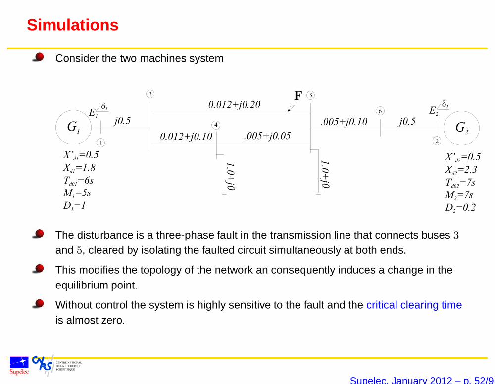
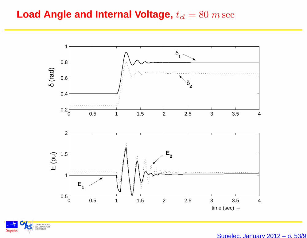
Simulations
Consider the two machines system
3
1
5
6
4
2
j0.5
0.012+j0.10
0.012+j0.20
.005+j0.05
.005+j0.10 j0.5E2
d2
1.0
+j0
1.0
+j0
G2G1
E1
d1
F
X’ =0.5
X =1.8
T =6s
M =5s
d1
d1
d01
1
D =11
X’ =0.5
X =2.3
T =7s
M =7s
D =0.2
d2
d2
d02
2
2
The disturbance is a three-phase fault in the transmission line that connects buses 3
and 5, cleared by isolating the faulted circuit simultaneously at both ends.
This modifies the topology of the network an consequently induces a change in theequilibrium point.
Without control the system is highly sensitive to the fault and the critical clearing timeis almost zero.
Supelec, January 2012 – p. 52/91
CENTRE NATIONAL DE LA RECHERCHESCIENTIFIQUE
Load Angle and Internal Voltage, tcl = 80 m sec
0 0.5 1 1.5 2 2.5 3 3.5 40.2
0.4
0.6
0.8
1δ
(rad
)
0 0.5 1 1.5 2 2.5 3 3.5 40.5
1
1.5
2
time (sec) →
E (
pu)
δ1
δ2
E1
E2
Supelec, January 2012 – p. 53/91
CENTRE NATIONAL DE LA RECHERCHESCIENTIFIQUE
Other Results
Derivation of a Lyapunov function for the full model (Zonetti, et al., ACC’12).
Actuation via flexible AC transmission systems, (Manjarekar, et al., Electrical PowerSystems Research’10, EJC’11).
Structure preserving models
Cyclo-dissipativity properties have been established and a linear controllerproposed – leads to an LMI test, (Guisto, et al., CDC’08).
“Full solution" using Lyapunov–based designs (Dib, et al., TAC’10), (Casagrande,et al., CDC’11).
Alternative formulation as a synchronization, not stabilization, problem, (Dib, et al.,ACC’11).
Immersing a pendular dynamics.
Existence solution for n machines.
Supelec, January 2012 – p. 54/91

CENTRE NATIONAL DE LA RECHERCHESCIENTIFIQUE
Electromechanical Systems
Supelec, January 2012 – p. 55/91
CENTRE NATIONAL DE LA RECHERCHESCIENTIFIQUE
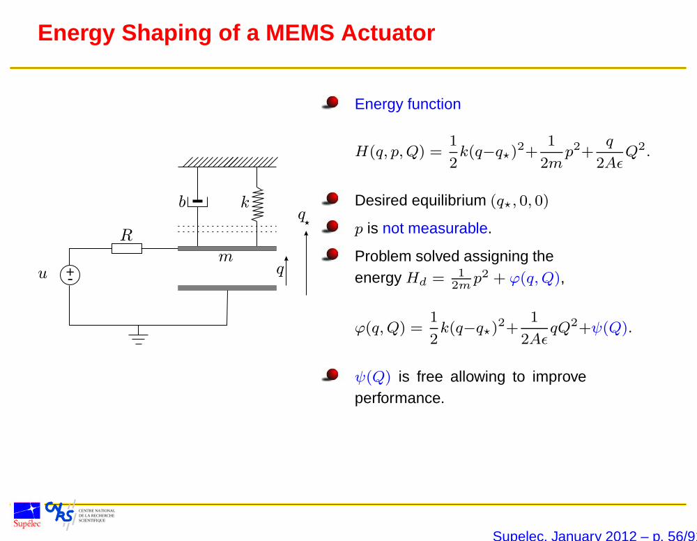
Energy Shaping of a MEMS Actuator
b k
u
R
q
q
m+-
Energy function
H(q, p,Q) =1
2k(q−q?)
2+1
2mp2+
q
2AεQ2.
Desired equilibrium (q?, 0, 0)
p is not measurable.
Problem solved assigning theenergy Hd = 1
2mp2 + ϕ(q,Q),
ϕ(q,Q) =1
2k(q−q?)
2+1
2AεqQ2+ψ(Q).
ψ(Q) is free allowing to improveperformance.
Supelec, January 2012 – p. 56/91
CENTRE NATIONAL DE LA RECHERCHESCIENTIFIQUE
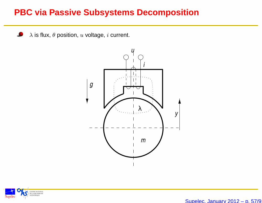
PBC via Passive Subsystems Decomposition
λ is flux, θ position, u voltage, i current.
u
i
y
g
m
λ
Supelec, January 2012 – p. 57/91
CENTRE NATIONAL DE LA RECHERCHESCIENTIFIQUE
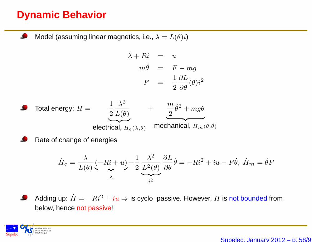
Dynamic Behavior
Model (assuming linear magnetics, i.e., λ = L(θ)i)
λ+ Ri = u
mθ = F −mg
F =1
2
∂L
∂θ(θ)i2
Total energy: H =1
2
λ2
L(θ)︸ ︷︷ ︸
electrical, He(λ,θ)
+m
2θ2 +mgθ
︸ ︷︷ ︸mechanical, Hm(θ,θ)
Rate of change of energies
He =λ
L(θ)(−Ri+ u)︸ ︷︷ ︸
λ
−1
2
λ2
L2(θ)︸ ︷︷ ︸
i2
∂L
∂θθ = −Ri2 + iu− F θ, Hm = θF
Adding up: H = −Ri2 + iu⇒ is cyclo–passive. However, H is not bounded frombelow, hence not passive!
Supelec, January 2012 – p. 58/91
CENTRE NATIONAL DE LA RECHERCHESCIENTIFIQUE
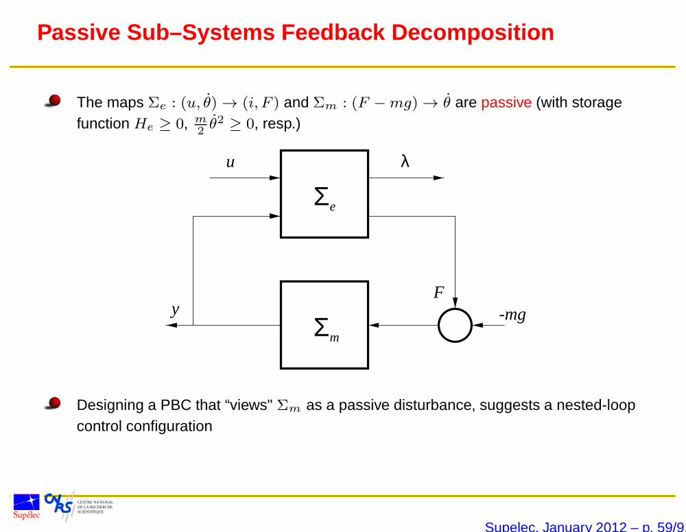
Passive Sub–Systems Feedback Decomposition
The maps Σe : (u, θ) → (i, F ) and Σm : (F −mg) → θ are passive (with storagefunction He ≥ 0, m
2θ2 ≥ 0, resp.)
u
F-mgy
λ
Σ
Σ
e
m
Designing a PBC that “views" Σm as a passive disturbance, suggests a nested-loopcontrol configuration
Supelec, January 2012 – p. 59/91
CENTRE NATIONAL DE LA RECHERCHESCIENTIFIQUE
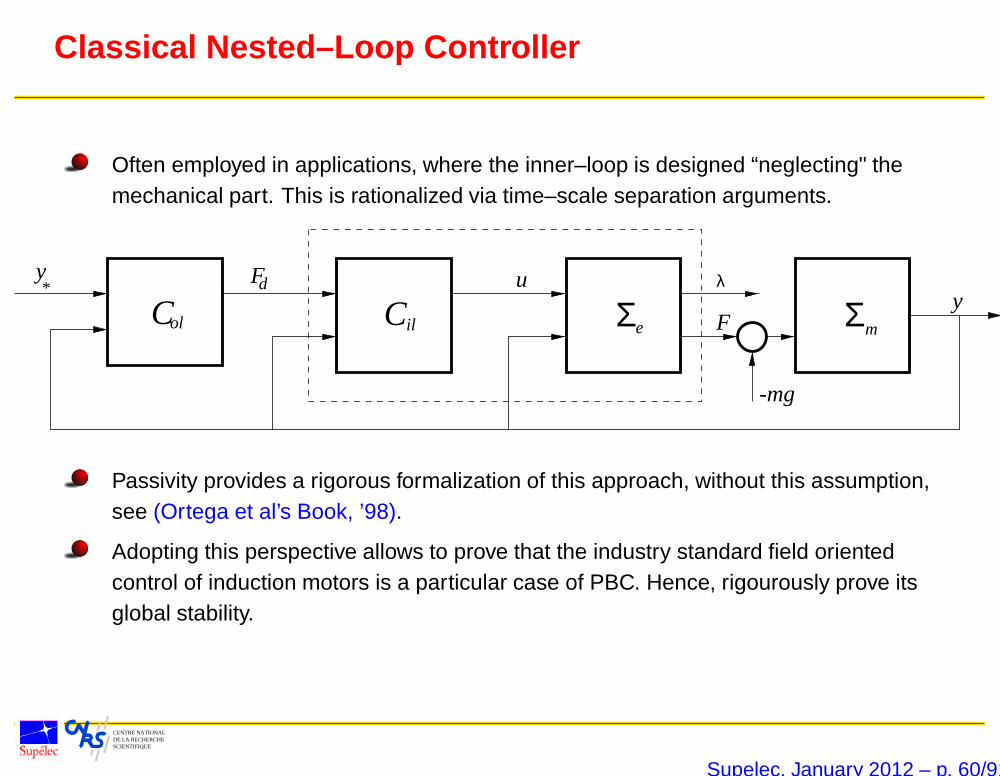
Classical Nested–Loop Controller
Often employed in applications, where the inner–loop is designed “neglecting" themechanical part. This is rationalized via time–scale separation arguments.
yu
F
-mg
λ
Col
Fd
Cil Σe Σm
y*
Passivity provides a rigorous formalization of this approach, without this assumption,see (Ortega et al’s Book, ’98).
Adopting this perspective allows to prove that the industry standard field orientedcontrol of induction motors is a particular case of PBC. Hence, rigourously prove itsglobal stability.
Supelec, January 2012 – p. 60/91
CENTRE NATIONAL DE LA RECHERCHESCIENTIFIQUE
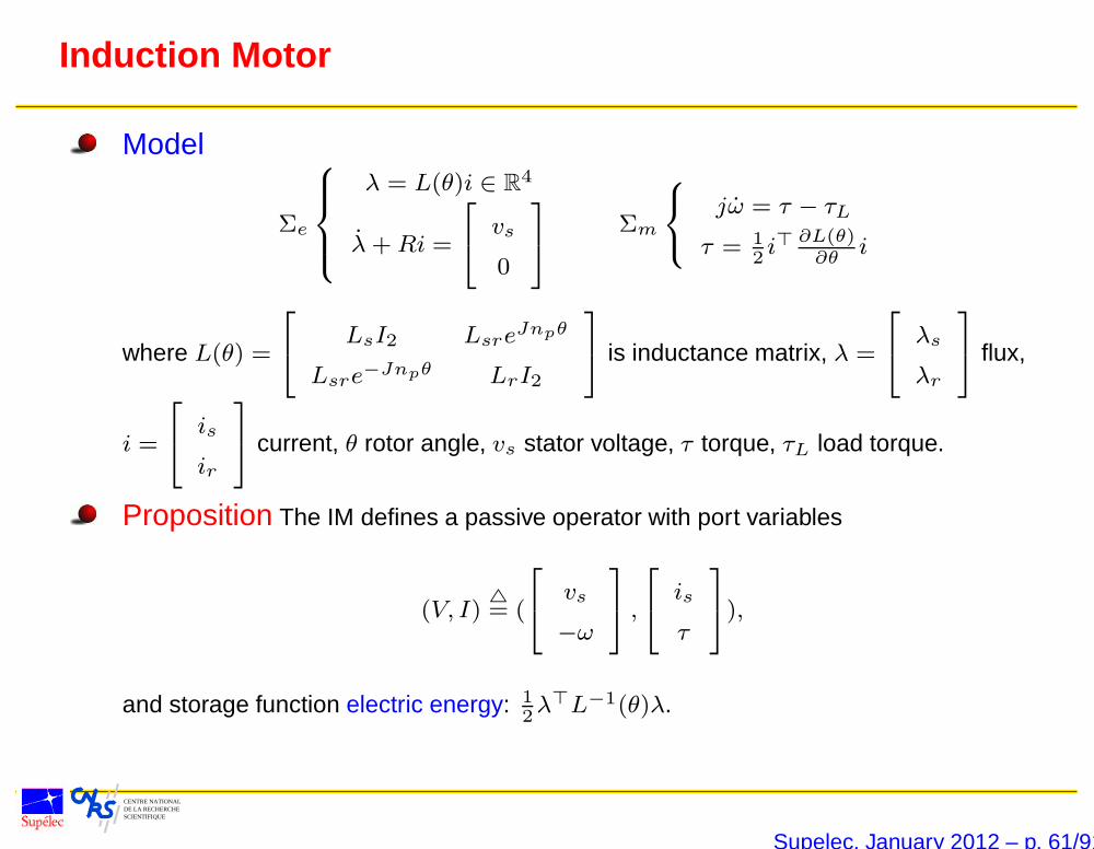
Induction Motor
Model
Σe
λ = L(θ)i ∈ R4
λ+Ri =
vs
0
Σm
jω = τ − τL
τ = 12i>
∂L(θ)∂θ
i
where L(θ) =
LsI2 Lsre
Jnpθ
Lsre−Jnpθ LrI2
is inductance matrix, λ =
λs
λr
flux,
i =
is
ir
current, θ rotor angle, vs stator voltage, τ torque, τL load torque.
Proposition The IM defines a passive operator with port variables
(V, I)4= (
vs
−ω
,
is
τ
),
and storage function electric energy: 12λ>L−1(θ)λ.
Supelec, January 2012 – p. 61/91
CENTRE NATIONAL DE LA RECHERCHESCIENTIFIQUE
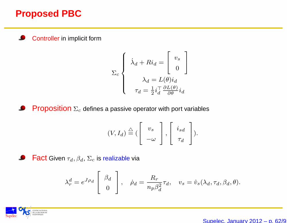
Proposed PBC
Controller in implicit form
Σc
λd +Rid =
vs
0
λd = L(θ)id
τd = 12i>d
∂L(θ)∂θ
id
Proposition Σc defines a passive operator with port variables
(V, Id)4= (
vs
−ω
,
isd
τd
).
Fact Given τd, βd, Σc is realizable via
λdr = eJρd
βd
0
, ρd =
Rr
npβ2d
τd, vs = vs(λd, τd, βd, θ).
Supelec, January 2012 – p. 62/91
CENTRE NATIONAL DE LA RECHERCHESCIENTIFIQUE
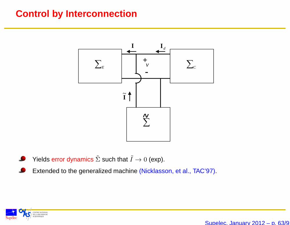
Control by Interconnection
∑E
∑C
∑
I dI
v -
+
I~
Yields error dynamics Σ such that I → 0 (exp).
Extended to the generalized machine (Nicklasson, et al., TAC’97).
Supelec, January 2012 – p. 63/91
CENTRE NATIONAL DE LA RECHERCHESCIENTIFIQUE
Some Additional Results
Sensorless control of PMSM with guaranteed stability properties, (Shah, et al.,IFAC’11).
PBC of doubly–fed induction machines, for energy management applications (Battle, etal., EJC’07).
CbI of doubly–fed induction machines, (Battle, et al., IJC’11).
Supelec, January 2012 – p. 64/91

CENTRE NATIONAL DE LA RECHERCHESCIENTIFIQUE
Dynamic Energy Router
Supelec, January 2012 – p. 65/91
CENTRE NATIONAL DE LA RECHERCHESCIENTIFIQUE
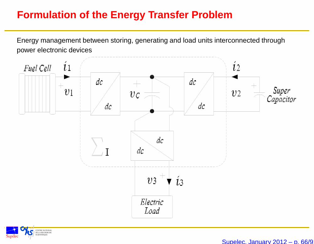
Formulation of the Energy Transfer Problem
Energy management between storing, generating and load units interconnected throughpower electronic devices
Supelec, January 2012 – p. 66/91
CENTRE NATIONAL DE LA RECHERCHESCIENTIFIQUE
Current Practice, Limitations and Objective
Assume that system operates in steady state
Translate power demand into current or voltage references
Track references with PI controllers in the power converters
Discriminate between fast and slow changing power demand via linear filtering
⇒ Behavior below par during transients and for fast changing demands
Our objective is to propose a ΣI that
Does not rely on steady–state considerations
Allows to incorporate dynamic restrictions of the units
Handles dissipation
Supelec, January 2012 – p. 67/91
CENTRE NATIONAL DE LA RECHERCHESCIENTIFIQUE
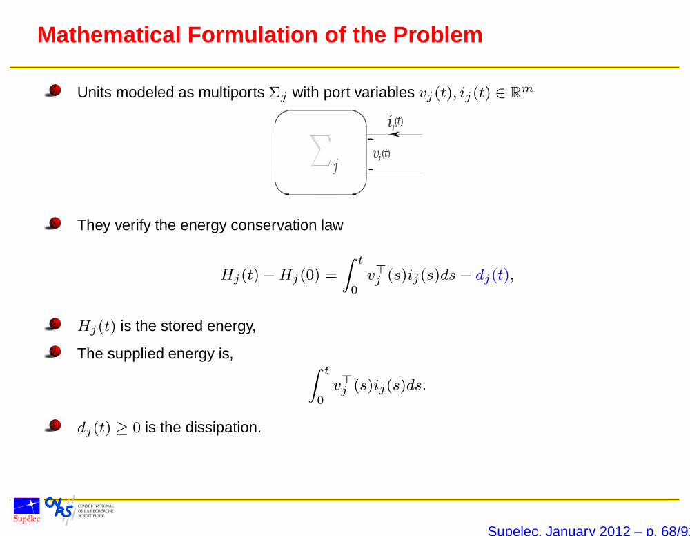
Mathematical Formulation of the Problem
Units modeled as multiports Σj with port variables vj(t), ij(t) ∈ Rm
They verify the energy conservation law
Hj(t)−Hj(0) =
∫ t
0v>j (s)ij(s)ds− dj(t),
Hj(t) is the stored energy,
The supplied energy is, ∫ t
0v>j (s)ij(s)ds.
dj(t) ≥ 0 is the dissipation.
Supelec, January 2012 – p. 68/91
CENTRE NATIONAL DE LA RECHERCHESCIENTIFIQUE
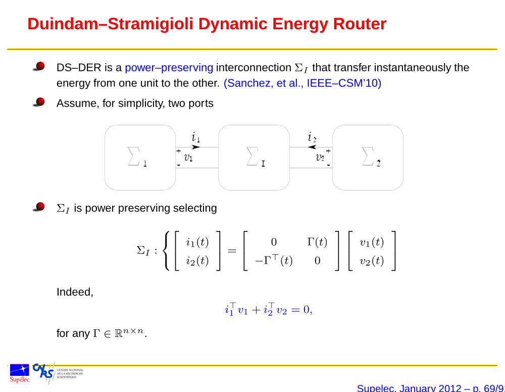
Duindam–Stramigioli Dynamic Energy Router
DS–DER is a power–preserving interconnection ΣI that transfer instantaneously theenergy from one unit to the other. (Sanchez, et al., IEEE–CSM’10)
Assume, for simplicity, two ports
ΣI is power preserving selecting
ΣI :
i1(t)
i2(t)
=
0 Γ(t)
−Γ>(t) 0
v1(t)
v2(t)
Indeed,
i>1 v1 + i>2 v2 = 0,
for any Γ ∈ Rn×n.
Supelec, January 2012 – p. 69/91
CENTRE NATIONAL DE LA RECHERCHESCIENTIFIQUE
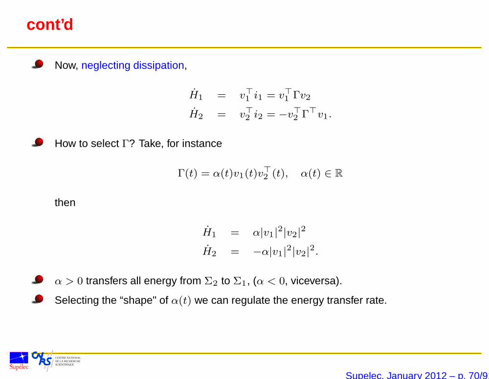
cont’d
Now, neglecting dissipation,
H1 = v>1 i1 = v>1 Γv2
H2 = v>2 i2 = −v>2 Γ>v1.
How to select Γ? Take, for instance
Γ(t) = α(t)v1(t)v>2 (t), α(t) ∈ R
then
H1 = α|v1|2|v2|
2
H2 = −α|v1|2|v2|
2.
α > 0 transfers all energy from Σ2 to Σ1, (α < 0, viceversa).
Selecting the “shape" of α(t) we can regulate the energy transfer rate.
Supelec, January 2012 – p. 70/91
CENTRE NATIONAL DE LA RECHERCHESCIENTIFIQUE
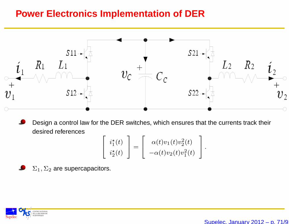
Power Electronics Implementation of DER
Design a control law for the DER switches, which ensures that the currents track theirdesired references
i?1(t)
i?2(t)
=
α(t)v1(t)v22(t)
−α(t)v2(t)v21(t)
.
Σ1,Σ2 are supercapacitors.
Supelec, January 2012 – p. 71/91
CENTRE NATIONAL DE LA RECHERCHESCIENTIFIQUE
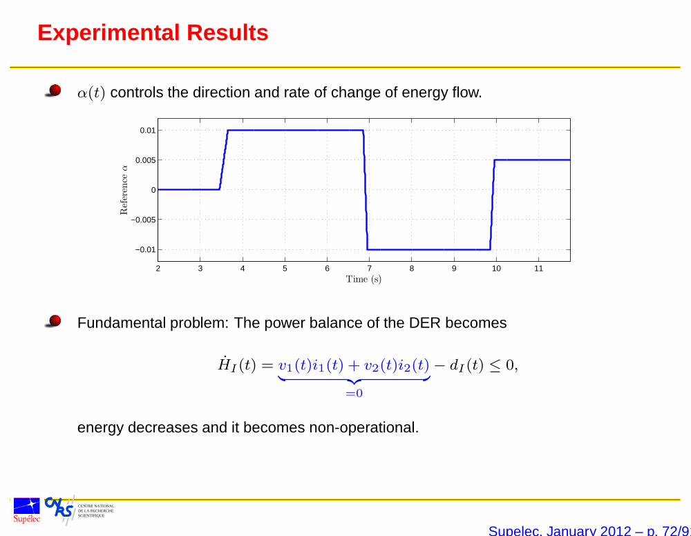
Experimental Results
α(t) controls the direction and rate of change of energy flow.
2 3 4 5 6 7 8 9 10 11
−0.01
−0.005
0
0.005
0.01R
efer
enceα
Time (s)
Fundamental problem: The power balance of the DER becomes
HI(t) = v1(t)i1(t) + v2(t)i2(t)︸ ︷︷ ︸=0
− dI(t) ≤ 0,
energy decreases and it becomes non-operational.
Supelec, January 2012 – p. 72/91
CENTRE NATIONAL DE LA RECHERCHESCIENTIFIQUE
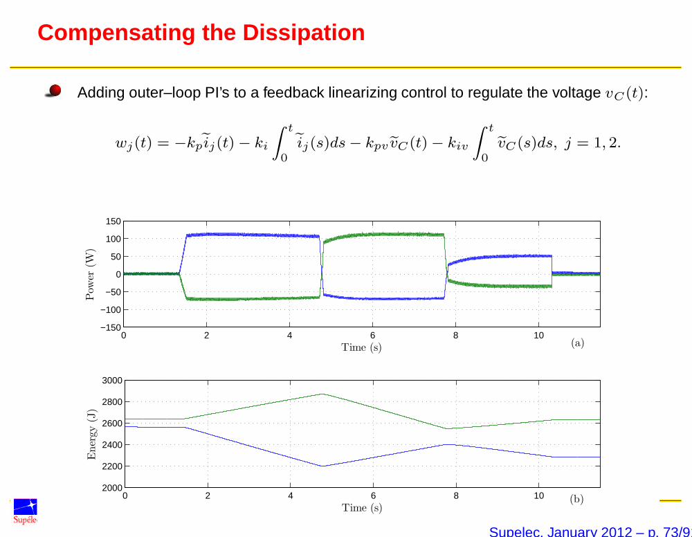
Compensating the Dissipation
Adding outer–loop PI’s to a feedback linearizing control to regulate the voltage vC(t):
wj(t) = −kp ij(t)− ki
∫ t
0ij(s)ds− kpv vC(t)− kiv
∫ t
0vC(s)ds, j = 1, 2.
0 2 4 6 8 10−150
−100
−50
0
50
100
150
Pow
er(W
)
Time (s) (a)
0 2 4 6 8 102000
2200
2400
2600
2800
3000
En
ergy
(J)
Time (s)(b)
Supelec, January 2012 – p. 73/91
CENTRE NATIONAL DE LA RECHERCHESCIENTIFIQUE
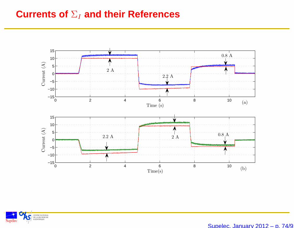
Currents of ΣI and their References
0 2 4 6 8 10−15
−10
−5
0
5
10
15
Cu
rren
t(A
)
Time (s)(a)
0 2 4 6 8 10−15
−10
−5
0
5
10
15
Cu
rren
t(A
)
Time(s)(b)
2.2 A
2.2 A
2 A
2 A0.8 A
0.8 A
Supelec, January 2012 – p. 74/91

CENTRE NATIONAL DE LA RECHERCHESCIENTIFIQUE
Voltage of DC Link
0 2 4 6 8 100
5
10
15
20
Vol
tage
(V)
Time (s)
Supelec, January 2012 – p. 75/91

CENTRE NATIONAL DE LA RECHERCHESCIENTIFIQUE
Proposed Solution: Abandon Power Preservation
Define mappings Fj(v) for the current references:
i?j (t) = Fj(v(t)), j ∈ N ,
Two different objectives:
Ensure the desired power dispatch, P ?j (t) = v>j (t)Fj(v(t)).
Compensate dissipation,∑N
j=1 v>j (t)Fj(v(t)) = dI (t).
Possible choice
Fj(v) = δjΠNk=1,k 6=j |vk|
2vj ,
N∑
j=1
δj(t) = dI(t).
If |vj(t)| ≥ ε > 0, fix
Fj(vj(t)) =P ?j (t)
|vj(t)|2vj(t),
with∑N
j=1 P?j (t) = dI(t).
Supelec, January 2012 – p. 76/91
CENTRE NATIONAL DE LA RECHERCHESCIENTIFIQUE
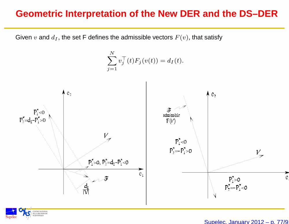
Geometric Interpretation of the New DER and the DS–DER
Given v and dI , the set F defines the admissible vectors F (v), that satisfy
N∑
j=1
v>j (t)Fj(v(t)) = dI (t).
Supelec, January 2012 – p. 77/91
CENTRE NATIONAL DE LA RECHERCHESCIENTIFIQUE
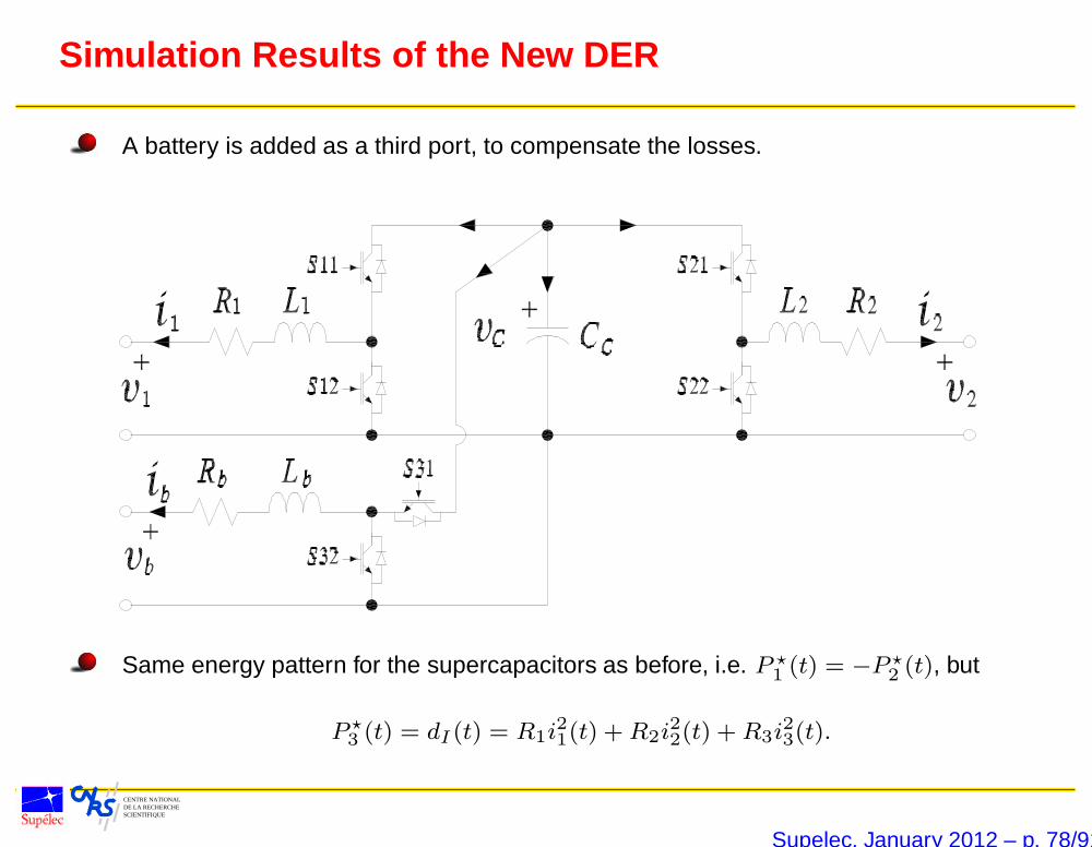
Simulation Results of the New DER
A battery is added as a third port, to compensate the losses.
Same energy pattern for the supercapacitors as before, i.e. P ?1 (t) = −P ?
2 (t), but
P ?3 (t) = dI (t) = R1i
21(t) + R2i
22(t) + R3i
23(t).
Supelec, January 2012 – p. 78/91
CENTRE NATIONAL DE LA RECHERCHESCIENTIFIQUE
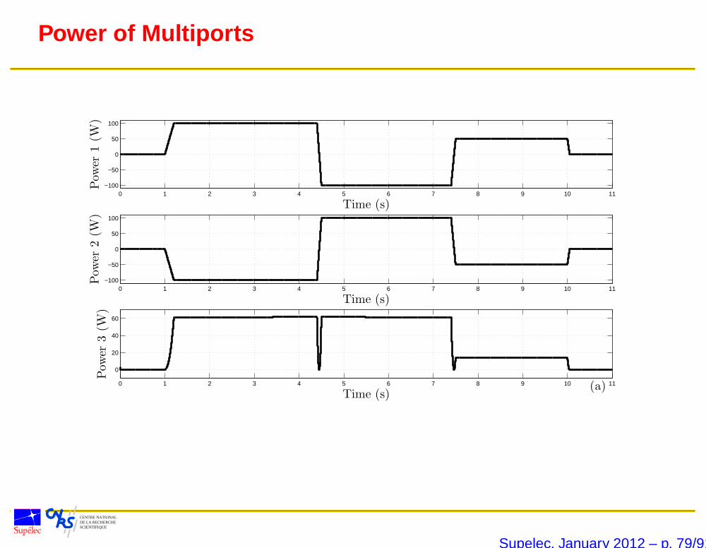
Power of Multiports
0 1 2 3 4 5 6 7 8 9 10 11−100
−50
0
50
100
Pow
er1
(W)
Time (s)
0 1 2 3 4 5 6 7 8 9 10 11−100
−50
0
50
100
Pow
er2
(W)
Time (s)
0 1 2 3 4 5 6 7 8 9 10 11
0
20
40
60
Pow
er3
(W)
Time (s)(a)
Supelec, January 2012 – p. 79/91
CENTRE NATIONAL DE LA RECHERCHESCIENTIFIQUE
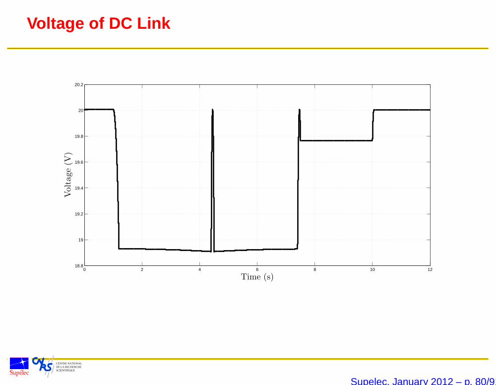
Voltage of DC Link
0 2 4 6 8 10 1218.8
19
19.2
19.4
19.6
19.8
20
20.2
Volt
age
(V)
Time (s)
Supelec, January 2012 – p. 80/91

CENTRE NATIONAL DE LA RECHERCHESCIENTIFIQUE
Some Additional Results
Power factor compensation is equivalent to cyclo–dissipasivation: The nonlinearnon–sinusoidal case, (Garcia, et al., IEEE-CSM’07).
Proof of passivity of a PEM fuel cell model, (Talj and Ortega, Automatica’11).
Passivity and robust PI control of the air supply system of a PEM fuel cell model, (Talj,et al., IEEE TIE’10).
Supelec, January 2012 – p. 81/91

CENTRE NATIONAL DE LA RECHERCHESCIENTIFIQUE
Wind Speed Estimation in WindmillSystems
Supelec, January 2012 – p. 82/91
CENTRE NATIONAL DE LA RECHERCHESCIENTIFIQUE
Mathematical Model of the Windmill System
System is a wind turbine and a generator.
The mechanical dynamics,
Jωm = Tm − Te, (Σ)
with J the rotor inertia, P is the number of pole pairs, ωm the mechanical speed, Tethe electrical torque, and the mechanical torque
Tm =Pw
ωm.
The mechanical power at the windmill shaft
Pw =1
2ρACp(
rωm
vw)v3w,
with Cp(λ), λ := rωm
vw, the power coefficient and vw the unknown wind speed, which
enters nonlinearly.
Supelec, January 2012 – p. 83/91
CENTRE NATIONAL DE LA RECHERCHESCIENTIFIQUE
Assumptions for Wind Speed Estimation
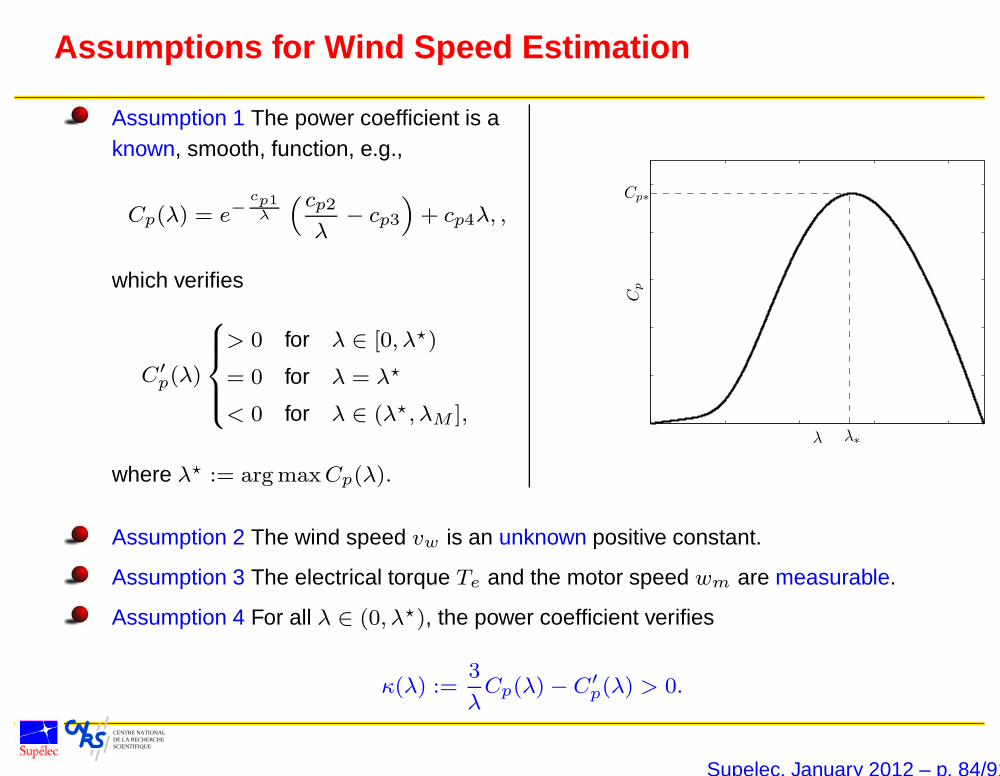
Assumption 1 The power coefficient is aknown, smooth, function, e.g.,
Cp(λ) = e−cp1λ
( cp2λ
− cp3
)+ cp4λ, ,
which verifies
C′p(λ)
> 0 for λ ∈ [0, λ?)
= 0 for λ = λ?
< 0 for λ ∈ (λ?, λM ],
where λ? := argmaxCp(λ).
λ
Cp
λ∗
Cp∗
Assumption 2 The wind speed vw is an unknown positive constant.
Assumption 3 The electrical torque Te and the motor speed wm are measurable.
Assumption 4 For all λ ∈ (0, λ?), the power coefficient verifies
κ(λ) :=3
λCp(λ)− C′
p(λ) > 0.
Supelec, January 2012 – p. 84/91
CENTRE NATIONAL DE LA RECHERCHESCIENTIFIQUE
Some Remarks
Cp(λ) can be easily obtained from experimental data, and the algorithm implementedfrom a table look–up.
Constant wind speed assumption only needed for the theory. An on–line estimator isable to track slowly–varying parameters, assumption justified by the time scaleseparation between the wind dynamics and the mechanical and electrical signals.
On–line estimators average the noise—in contrast with differentiator–based orextended Kalman filter schemes currently used.
Measuring wm and Te is standard practice in windmill systems.
Theory applicable also if blade pitch β is included, i.e., Cp(λ, β), or for more completedescriptions of the mechanical dynamics.
Assumption 4 is satisfied in normal operating range (for Region 2), where the torquecoefficient has negative slope. Indeed,
CT (λ) :=1
λCp(λ),
satisfies
C′T (λ) ≤ 0 ⇒ Assumption 4.
Supelec, January 2012 – p. 85/91
CENTRE NATIONAL DE LA RECHERCHESCIENTIFIQUE
Immersion and Invariance Parameter Estimators
Proposition (Liu, et al., TAC’10, SCL’11) Consider the system
x = F (t) + Φ(x, θ),
where x ∈ R, the function F (t) and the mapping Φ : R× R → R are known, and θ ∈ R is aconstant unknown parameter. Assume there exists a smooth mapping β : R → R such thatthe parameterized mapping
Qx(θ) := β′(x)Φ(x, θ)
is strictly monotone increasing. The I&I estimator
˙θI = −β′(x)
[F (t) + Φ(x, θI + β(x))
]
θ = θI + β(x),
is asymptotically consistent. That is, limt→∞ θ(t) = θ. for all (x(0), θI(0)) ∈ R× R, andF (t) such that (x(t), θ(t)) exist for all t ≥ 0.
Supelec, January 2012 – p. 86/91

CENTRE NATIONAL DE LA RECHERCHESCIENTIFIQUE
Verifying the Monotonicity Condition
Apply Proposition with x = ωm, θ = ωm and F (t) = − 1JTe(t).
Key step is to construct a function β(·), such that the parameterized function
Qωm(vw) = β′(ωm)Φ(ωm, vw)
is strictly monotonically increasing.
The latter is true if and only if its derivative is positive,
Q′ωm
(vw) = β′(ωm)∂Φ(ωm, vw)
∂vw
=ρAr
2Jvwβ
′(ωm)
[3vw
rωm
Cp
(rωm
vw
)− C′
p
(rωm
vw
)].
The term in brackets, is precisely κ(λ), hence the need for Assumption 4.
Supelec, January 2012 – p. 87/91
CENTRE NATIONAL DE LA RECHERCHESCIENTIFIQUE
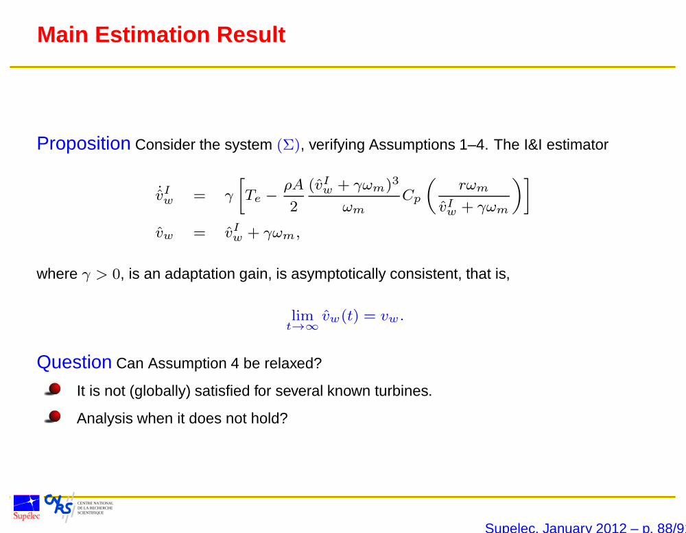
Main Estimation Result
Proposition Consider the system (Σ), verifying Assumptions 1–4. The I&I estimator
˙vIw = γ
[Te −
ρA
2
(vIw + γωm)3
ωm
Cp
(rωm
vIw + γωm
)]
vw = vIw + γωm,
where γ > 0, is an adaptation gain, is asymptotically consistent, that is,
limt→∞
vw(t) = vw.
Question Can Assumption 4 be relaxed?
It is not (globally) satisfied for several known turbines.
Analysis when it does not hold?
Supelec, January 2012 – p. 88/91
CENTRE NATIONAL DE LA RECHERCHESCIENTIFIQUE
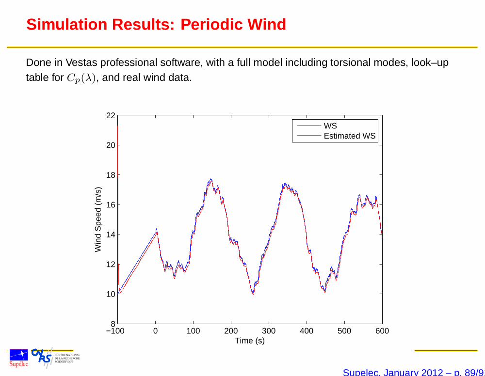
Simulation Results: Periodic Wind
Done in Vestas professional software, with a full model including torsional modes, look–uptable for Cp(λ), and real wind data.
−100 0 100 200 300 400 500 6008
10
12
14
16
18
20
22
Time (s)
Win
d S
peed
(m
/s)
WSEstimated WS
Supelec, January 2012 – p. 89/91
CENTRE NATIONAL DE LA RECHERCHESCIENTIFIQUE
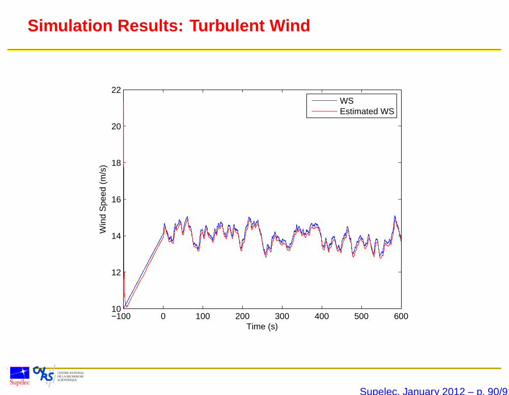
Simulation Results: Turbulent Wind
−100 0 100 200 300 400 500 60010
12
14
16
18
20
22
Time (s)
Win
d S
peed
(m
/s)
WSEstimated WS
Supelec, January 2012 – p. 90/91
CENTRE NATIONAL DE LA RECHERCHESCIENTIFIQUE
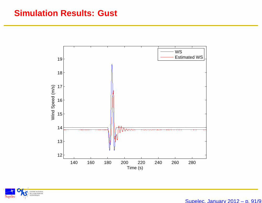
Simulation Results: Gust
140 160 180 200 220 240 260 280
12
13
14
15
16
17
18
19
Time (s)
Win
d S
peed
(m
/s)
WSEstimated WS
Supelec, January 2012 – p. 91/91