Embed Size (px)
Citation preview
A New Bayesian Unit Root Test in Stochastic
Volatility Models∗
Yong LiSun Yat-Sen University
Jun YuSingapore Management University
October 21, 2011
Abstract: A new posterior odds analysis is proposed to test for a unit root in volatility
dynamics in the context of stochastic volatility models. Our analysis extends the Bayesian
unit root test of So and Li (1999, Journal of Business and Economic Statistics)
in the two important ways. First, a numerically more stable algorithm is introduced to
compute Bayes factors, taking into account the special structure of the competing models.
Owing to its numerical stability, the algorithm overcomes the problem of the diverging
“size” in the marginal likelihood approach. Second, to improve the “power” of the unit
root test, a mixed prior specification with random weights is employed. It is shown that the
posterior odds ratio is the by-product of Bayesian estimation and can be easily computed
by MCMC methods. A simulation study examines the “size” and “power” performances
of the new method. An empirical study, based on time series data covering the subprime
crisis, reveals some interesting results.
Keywords: Bayes factor; Mixed Prior; Markov Chain Monte Carlo; Posterior odds ratio;
Stochastic volatility models; Unit root testing.
∗Li gratefully acknowledges the financial support of the Chinese Natural Science fund (No.70901077),the Chinese Education Ministry Social Science fund (No. 09YJC790266), the Fundamental Research Fundsfor the Central Universities and the hospitality during his research visits to Sim Kee Boon Institute forFinancial Economics at Singapore Management University. We would like to thank three referees fortheir constructive comments. Yong Li, Sun Yat-Sen Business School, Sun Yat-Sen University, Guangzhou,510275, China. Jun Yu, Sim Kee Boon Institute for Financial Economics, School of Economics and LeeKong Chian School of Business, Singapore Management University, 90 Stamford Road, Singapore 178903.Email: [email protected]. URL: http://www.mysmu.edu/faculty/yujun/.
1
1 Introduction
Whether or not there is a unit root in volatility of financial assets has been a long-standing
topic of interest to econometricians and empirical economists. There are several reasons
for this attention. First, the property of unit root has important implications for the
risk premium and asset allocations. For example, compared to a stationary volatility,
volatility with a unit root implies a stronger negative relation between the return and the
volatility (Chou, 1988). When there is a unit root in volatility, a rational investor should
constantly and permanently change the weighting of assets whenever a volatility shock
arrives. Second, motivated from the fact that volatility of financial assets is typically highly
persistent, econometric models which allow for a unit root in volatility have appeared.
Leading examples include the IGARCH model of Engle and Bollerslev (1986) and the log-
normal stochastic volatility (SV) model of Harvey et al. (1994). However, there is mixed
empirical evidence as to whether non-stationarity exists in volatility. Third, if there is
a unit root in volatility, the frequentist’s inference, which is often based on asymptotic
theory, is often more much complicated; see, for example, Park and Phillips (2001) and
Bandi and Phillips (2003) for the development of asymptotic theory for nonlinear models
with a unit root.
In a log-normal SV model, the volatility is often assumed to follow an AR(1) model
with the autoregressive coefficient ϕ. The test of unit root amounts to testing ϕ = 1.
The estimation of ϕ is complicated by the fact that volatility is latent. In recent years,
numerous estimation methods have been developed to estimate SV model; see, Shephard
(2005) for a review. It is possible to test for a unit root in volatility without estimate the
entire SV model, however. Harvey et al. (1994) suggested a classical unit root test by
estimating ϕ in the log-squared return process. There are two problems with such a test.
First, ϕ is less efficiently estimated. Second, all the classical unit root tests suffer from
large size distortions because the log-squared return process follows an ARMA(1,1) model
with a large negative MA root. This problem is well known in the unit root literature; see,
for example, Schwert (1989). To overcome the second problem, Wright (1999) proposed
to use the unit root test of Perron and Ng (1996). The severe distortion in size is nicely
mitigated although there are still some distortions left in some parameter settings.
To deal with the first problem, So and Li (1999, SL hereafter) proposed a Bayesian unit
root test approach based on the Bayes factor (BF). The test is implemented in two stages.
At stage 1, the two competing models are estimated by the Bayesian MCMC method.
As a full likelihood-based method, MCMC provides a more efficient estimate of ϕ than
2
the least squares estimate and other frequentist’s estimates of ϕ in the log-squared
return process, provided the model is corrected specified; see Andersen et al. (1999).
At stage 2, the BF is obtained from the MCMC samples. The BF is an important statistic
in the Bayesian literature and has served as the gold standard for Bayesian model testing
and comparison for a long time (Kass and Raftery, 1995; Geweke, 2007). However, it is
necessary to point out that the impact of prior specifications on BF is different from that on
estimation. For estimation, it is well-known that in large samples, prior distributions can
be picked for convenience because their effects on posterior distributions are insignificant
(Kass and Raftery, 1995). For BF, standard improper noninformative priors can not
be applied since such priors are defined only up to a constant, hence the resulting BF
is a multiple of an arbitrary constant. In fact, as pointed out by Kass and Raftery, if
a prior with a very large spread is used on some parameter under a model to make it
“noninformative”, this behavior will force the BF to favor its competitive model. This
problem is well-known as Jeffreys-Lindley-Bartlett’s paradox in the Bayesian literature.
Consequently, it should be very careful to apply the noninformative prior for a unit root
testing problem.
To avoid the difficulty, the prior distributions are generally taken to be proper and not
have too big a spread. Moreover, it is often suggested that for Bayesian model comparison,
an equal model prior should be used. This practice was followed by SL. However, it is
now known in the unit root literature that if a proper prior is adopted for parameters
and an equal weight is used to represent the prior model ignorance, there is a bias toward
stationary models; see, for example, Phillips (1991) and Ahking (2008). To alleviate this
problem, our first contribution of the paper is to propose a mixed prior distribution with
a random weight for the unit root test. The main idea is that when the prior information
is not available, we can obtain an estimate for the random weight when a vague prior is
assigned. If the data are generated from a unit root process, it can be expected that a
larger weight is assigned to the unit root process. In other words, we use it to adjust the
bias towards stationarity in the posterior odds analysis for unit root with the estimated
weight. This idea is related to what was proposed by Kalaylioglu and Ghosh
(2009). However, a key difference between our work and theirs is that we use
the BF to compare the competing models while Kalaylioglu and Ghosh used
the Bayesian credible interval.
Our second contribution lies in the computation of the BF. The computation of the BF
often involves high-dimensional integration and hence numerically demanding. SL applied
the marginal likelihood approach proposed by Chib (1995) to estimate the BF for the unit
3
root test. This approach is very general and has a very wide applicability. However, for
the SV models, the dimension of the parameters and the latent volatilities is very high,
the marginalization of the joint probability density over the parameters and the latent
variable poses a formidable computational challenge. In this paper, instead of calculating
the marginal likelihood, we derive a novel form for the BF by taking into account the
special structure of the competing models. In the new form, no marginalization is needed
and hence numerically it is more stable. It is shown that this evaluation of the BF in
the new form is a by-product of Bayesian MCMC estimation and hence it is trivial to
compute. This idea is related to Jacquier et al. (2004), Kou et al. (2005) and
Nicolae et al. (2008).
Our third contribution is that we perform the unit root test in a more general model
which allows for a fat-tailed conditional distribution and use real data from a period which
cover the recent subprime crisis. This test under this general set-up and with new data
suggests that the unit root model is more difficult to reject.
The remainder of this paper is organized as follows. In Section 2, we describe the
simple log-normal SV model and the problem of the unit root test. In Section 3, the new
approach for the posterior odds analysis of unit root is discussed. The performance of the
proposed unit root test procedure is examined using simulation data in Section 4. Section
5 considers some empirical applications. This paper is concluded in Section 6.
2 Stochastic Volatility Models
The simple log-normal SV model is of the form:
yt = exp(ht/2)ut, ut ∼ N(0, 1), (1)
ht = τ + ϕ(ht−1 − τ) + σvt, vt ∼ N(0, 1), (2)
where t = 1, 2, · · · , n, yt is the continuously compounded return, ht the unobserved log-
volatility, h0 ∼ N(τ, σ2
1−ϕ2
)when |ϕ| < 1, h0 ∼ N(τ, σ2) when ϕ = 1, and (ut, ηt) inde-
pendently standard normal variables for all t. This model can explain several important
stylized facts in the financial time series including volatility clustering, and its continuous
time version has been used to price options.
The primary concern of our paper is to test ϕ = 1 against |ϕ| < 1. SL (1999) proposed
a test by first estimating two competing models by a powerful MCMC algorithm – Gibbs
sampler. This Bayesian simulation based method generates samples from the joint pos-
terior distribution of the parameters and the latent volatility (so the data augmentation
4
technique is adopted here). After that, the posterior odds ratio was calculated using the
marginal likelihood method of Chib (1995).
To fixed the idea, let p(θ) be the prior distribution of the unknown parameter θ
(:= (τ, σ, ϕ) or (τ, σ) in the unit root case), y = (y1, · · · , yn) the observation vector,
h = (h1, · · · , hn) the vector of the latent variables. Exact maximum likelihood methods
are not possible because the likelihood p(y|θ) does not have a closed-form expression.
Bayesian methods overcome this difficulty by the data-augmentation strategy (Tanner and
Wong, 1987), namely, the parameter space is augmented from θ to (θ,h). By successive
conditioning and assuming prior independence in θ, the joint prior density is
p(τ, σ, ϕ,h) = p(τ)p(σ)p(ϕ)p(h0)
n∏t=1
p(ht|ht−1, θ). (3)
The likelihood function is
p(y|θ,h) =n∏
t=1
p(yt|ht). (4)
Obviously, both the joint prior density and the likelihood function are available analytically
provided analytical expressions for the prior distributions of θ are supplied. By Bayes’
theorem, the joint posterior distribution of the unobservables given the data is given by,
p(τ, σ, ϕ,h|y) ∝ p(τ)p(σ)p(ϕ)p(h0)n∏
t=1
p(ht|ht−1, θ)n∏
t=1
p(xt|ht). (5)
Gibbs sampler was used by SL to generate correlated samples from the joint posterior
distribution (5). In particular, it samples each variate, one at a time, from (5). When
all the variates are sampled in a cycle, we have one sweep. The algorithm is then re-
peated for many sweeps with the variates being updated with the most recent samples,
producing draws from Markov chains. With regularity conditions, the draws converge to
the posterior distribution at a geometric rate. By the ergodic theorem for Markov chains,
the posterior moments and marginal densities may be estimated by averaging the corre-
sponding functions over the sample. For example, one may estimate the posterior mean
by the sample mean, and obtain the credible interval from the marginal density. When the
simulation size is very large, the marginal densities can be regarded as the exact, enabling
exact finite sample inferences.
To explain the unit root test of SL, let M0 be the model formulated in the null hypoth-
esis (i.e. ϕ = 1), M1 the model formulated under the alternative hypothesis (i.e. ϕ is an
unknown parameter), π(Mk) the prior model probability density, p(y|Mk) the marginal
likelihood of model k, and p(Mk|y) the posterior probability densities, where k = 0, 1.
5
Under the Bayesian framework, testing the null hypothesis versus the alternative is equiv-
alent to comparing the two competing models, M0 versus M1. Given the prior model
probability density π(M0) and π(M1) = 1− π(M0), the data y produce a posterior model
density, p(M0|y) and p(M1|y) = 1− p(M0|y).Bayes’ theorem gives rise to
p(M0|y)p(M1|y)
=p(y|M0)
p(y|M1)× π(M0)
π(M1)(6)
that is
Posterior Odds Ratio (POR) = Bayes Factor (BF)× Prior Odds Ratio (7)
or
log01 (POR) = log01 (BF) + log01 (Prior Odds Ratio), (8)
where the BF is defined as the ratio of the marginal likelihood of the competing models.
If the prior odds is set to 1, as it is done in much of the Bayesian literature, the posterior
odds takes the same value as the BF. When the posterior odds is larger than 1, M0 is
favored over M1 and vice versus. In SL, the sign of log01(BF) was checked. If it is positive,
M0 is favored over M1. In general, one has to check the sign of log01(POR).
The marginal likelihood, p(y|Mk), can be expressed as
p(y|Mk) =
∫Ωk∪Ωh
p(y,h|θk,Mk)p(θk|Mk)dhdθk, (9)
where Ωk and Ωh are the support of θk and h, respectively. Alternatively, the marginal
likelihood can be expressed as
p(y|Mk) =
∫Ωk
p(y|θk,Mk)p(θk|Mk)dθk. (10)
As solving the integrals in (9) and (10) requires high-dimensional numerical integration,
Chib (1995) suggested evaluating the marginal likelihood by rearranging Bayes’ theorem
p(y|Mk) =p(y|θk,Mk)p(θk|Mk)
p(θk|y,Mk).
Thus, the log-marginal likelihood may be calculated by
ln p(y|θk,Mk) + ln p(θk|Mk)− ln p(θk|y,Mk) (11)
where θk is an appropriately selected high density point in estimated Mk and Chib sug-
gested using the posterior mean, θk. The first term of Equation (11) is the log-likelihood
6
evaluated at θk. Since it is marginalized over the latent volatilities, h, it is computationally
demanding and possibly numerically unstable. The second term is the log prior density
evaluated at θk and has to be specified by the econometrician. The third quantity involves
the posterior density which is only known up to a normality constant. The approximation
can be obtained by using a multivariate kernel density estimate based on the posterior
MCMC sample of θk.
To estimate θ, SL used the flat normal prior for τ , an inverse Gamma prior for σ2. For
ϕ, four different priors were used – uniform on the interval (0,1), truncated normal on (0,1),
two truncated Beta on (0,1). For the unit root test, the prior odds is set to 1. This choice
was argued to reflect prior ignorance. Simulation studies were conducted by SL to check
the performances of their Bayesian unit root test. While in general, their test perform
reasonably well, we identify we problems. First, the “size” diverges with the sample size.
Namely, when the sample size gets larger, the probability for the test to pick M0 when
the data are simulated from M0 is getting smaller. Since their empirical results suggest
that M1 is favored over M0, concerns about the diverged “size” are especially important.
Second, when ϕ is very close to 1, the test does not seem to have good “power” properties.
We argue that there is an obvious inconsistency between the choice of the prior of ϕ
and the choice of the prior odds. On the one hand, using a prior density whose support
exclude ϕ = 1 means that the researcher has no prior confidence about M0. On the other
hand, setting the prior odds to 1 implies that the researcher is equally confident about
the two competing model. It is well known in the unit root literature that the posterior
distribution is sensitive to the prior specification; see, for example, Phillips (1991), and
the discussion and the rejoinder in the same issue. From Equation (6) it is obvious that
the prior odds is important. As a result, it is reasonable to believe that the diverged “size”
may be due to the choice of the priors.
Consequently, we suggest two ways to improve the unit root test of SL. First, a com-
putationally easier and numerically more stable algorithm is introduced to compute the
BF, taking into account the special structure of the competing models. Our method com-
pletely avoids the calculation of marginal likelihood. Second, different priors for ϕ and
the model specification are employed. Our priors of ϕ allow for a positive mass at unity.
More important, a mixed model prior with random weights is used.
7
3 New Bayesian Unit Root Testing
3.1 A Set of Hierarchical Priors
Since we are concerned about the suitability of a prior for ϕ over (−1, 1) for the unit root
test, we first broaden the support of the prior distribution. In particular, we consider the
prior densities that assign a positive mass at unity. To be more specific, the prior is set to
f(ϕ) = πI(ϕ = 1) + (1− π)fC(ϕ)I(−1 < ϕ < 1), (12)
where I(x) is indicator function such that I(x) = 1 if x is true and 0 otherwise, π the
weight that represents the prior probability for model M0, and fC(ϕ) a proper distribution
that will be specified later. When π > 0, a positive mass is assignment to model M0.1The
mixed prior of this kind has been widely used in the unit root literature; see, for example,
Sims (1988) and Schotman and van Dijk (1991). In the SV literature, the same prior
was used in Kalaylioglu and Ghosh (2009).
As discussed before, when π(M0) = π(M1) = 0.5, POR takes the same value as the
BF, justifying the use of the BF for Bayesian model comparison. However, since we assign
probability π to model M0, when we specify the prior for ϕ, we have to assign π(M0) = π
to be logically consistent. In this case, the prior odds is π/(1− π). One choice for π is to
set π = 1/2. If so, POR is the same as the BF and we cannot improve the power of the
unit root test of SL. It is known in the unit root literature this prior tends favor stationary
or trend-stationary hypothesis; see, for example, Ahking (2008).
Alternatively, a uniform distribution over [0, 1] may be used for the hi-
erarchical specification of π to represent the prior ignorance. Based on the
mixture prior specification, Kalaylioglu and Ghosh (2009) used the posterior
confidence interval for unit root testing. Although the credible interval ap-
proach is simple to implement, it has some practical difficulties, as pointed
out in Robert (2002). First, the credible interval is not unique. Second, the
1In the unit root literature, for the autoregressive coefficient, an “objective” ignorance prior is the so-called Jeffreys or reference prior of Jeffreys (1961) and Berger and Bernardo (1992). As shown in Phillips(1991) these priors are intended to represent a state ignorance about the value of the autoregressioncoefficient and are very different from flat priors in the unit root testing problem. Unfortunately, thesepriors are improper and p(θk|Mk) = Ckf(θk) where f(θk) is a nonintegrable function and Ck is an arbitrarypositive constant. As a result the posterior odds can be rewritten as:
POR = BF =C0
C1
∫Ω0∪Ωh
p(y,h|θ0,M0)f(θ0)dhdθ0∫Ω1∪Ωh
p(y,h|θ1,M1)f(θ1)dhdθ1(13)
Thus, the posterior odds and the BF are not well defined since they both depend on the arbitrary constantsC0/C1. This is the reason why we decide not to use the Jeffrey’s prior to do the posterior odds analysisfor unit root.
8
credible interval approach typically does not have good behavior. Kalaylioglu
and Ghosh used the 95% symmetric posterior confidence interval for unit root
testing. Under the uniform hierarchical prior specification, it can be found
that, when the sample size was 500 and 1000, the “size” of the test is 0.21 and
0.11, suggesting the test is seriously distorted. Perhaps a better choice for
credible intervals is the highest posterior density (HPD) credible region. Un-
fortunately, the computation of the HPD credible region is usually demanding;
see Chen et al. (2000). In this paper, we deviate from Kalaylioglu and Ghosh
by using the posterior odds for unit root testing.
Ideally, a training sample should be selected to help determine the mean of π (denoted
by π), that may be used to compute the prior odds π/(1 − π). When π = 0.5, the POR
no longer takes the same value as the BF. If π > 0.5, log01(π/(1 − π)) > 0 and more
weight will be assigned to the positive mass at unity. In this case, compared with the BF,
the POR will favor more the unit root hypothesis. It is expected that this feature should
improve the power of the test because if data indeed come from a unit root model, it is
expected that π > 0.5. When data are generated from a stationary model, it is expected
that π < 0.5. Instead of splitting the entire sample into the training sample and the
sample for estimation, we estimate π from the entire sample in order to get the posterior
mean of π (say π), which is then used to compute the prior odds π/(1−π). By using the
same data to estimate the prior odds ratio and to calculate the BF, strictly
speaking, our approach is not a full Bayesian method. However, our proposed
idea shares the same spirit as that of Aitkin (1991) and Schotman and van
Dijk (1991). In Aitkin (1991) the data are re-used to get the prior distributions for the
parameters while in Schotman and van Dijk (1991) the threshold parameter of the defined
interval for ϕ is dependent on the data.
3.2 Computing Posterior Odds
Although the marginal likelihood approach proposed by Chib (1995) is very general and
has been applied in various studies (Kim, et al. 1998; Chib et al. 2002; Berg et al.
2004), it requires one to calculate the log-likelihood functions ln p(y|θk,Mk), k = 0, 1.
For the SV models, this is a challenging task. In this paper, we acknowledge that unit
root testing is a special model comparison problem which has the special structure to link
the competing models. The structure is that the two marginal likelihood functions have
the common latent variable which may be exploited to facilitate the computation of BF.
Instead of calculating the two marginal likelihood functions as suggested in Chib (1995),
9
in our method we only need to compute BF directly.
In a recent contribution, Jacquier, et al. (2004) proposed an efficient method to com-
pute BF for comparing the basic SV model with the fat-tailed SV model. They showed
that in the case the BF can be written as the expectation of the ratio of un-normalized
posteriors with respect to the posterior under the fat-tailed SV model. In addition,
Kou et al. (2005) and Nicolae et al. (2008) showed that for nested models, BF
can be written as the posterior mean of the likelihood ratio between the two
competing models. Here, we generalize these ideas by showing that the BF
for unit rooting testing also can be written as the complete likelihood ratio of
posterior quantities by introducing an appropriate weight function. To fix the
idea, let θ0 = (µ, σ2),θ1 = (µ, ϕ, σ2) and note that
B01 =
∫Ω0∪Ωh
p(θ0|M0)p(y,h|θ0,M0)
p(y|M1)dθ0dh
=
∫Ω1∪Ωh
p(θ0|M0)p(y,h|θ0,M0)w(ϕ|θ0)
p(y|M1)dϕdθ0dh
=
∫Ω1∪Ωh
p(θ0|M0)p(y,h|θ0,M0)w(ϕ|θ0)p(h,θ1|y,M1)
p(y,h,θ1|M1)dϕdθ1dh
=
∫Ω1∪Ωh
p(θ0|M0)w(ϕ|θ0)p(y,h|θ0,M0)
p(θ1|M1)p(y,h|θ1,M1)p(h,θ1|y,M1)dϕdθ1dh
where w(ϕ|θ0) is the an arbitrary weight function of ϕ conditional on θ0 such that∫w(ϕ|θ0)dϕ = 1
In practice, the prior distribution of the common parameter vector θ0 under two mod-
els is often specified as the same, that is p(θ0|M0) = p(θ0|M1). Furthermore, for the
purpose of the posterior odds analysis, p(ϕ|θ0,M1) is required to be a proper condi-
tional prior distribution. This distribution can be regarded as a weight function, then,
p(ϕ|θ0,M1)p(θ0|M1) = p(θ1|M1), hence,
B01 =
∫Ω1∪Ωh
p(θ0|M0)p(ϕ|θ0,M1)p(y,h|θ0,M0)
p(θ1|M1)p(y,h|θ1,M1)p(h,θ1|y,M1)dϕdθ1dh
=
∫Ω1∪Ωh
p(θ0|M1)p(ϕ|θ0,M1)p(y,h|θ0,M0)
p(θ1|M1)p(y,h|θ1,M1)p(h,θ1|y,M1)dϕdθ1dh
=
∫Ω1∪Ωh
p(y,h|θ0,M0)
p(y,h|θ1,M1)p(h,θ1|y,M1)dϕdθ1dh = E
p(y,h|θ0,M0)
p(y,h|θ1,M1)
(14)
where the expectation is with respect to the posterior distribution p(h,θ1|y,M1).
From (14), it can be seen that the BF is only a by-product of Bayesian estimation
of the SV model in the alternative hypothesis, namely, under the stationary case. Once
10
draws from Markov chains are available, the BF can be approximated conveniently and
efficiently by averaging over the MCMC draws. In fact, only one line of code is needed to
compute the BF. In detail, let h(s),θ(s)1 , s = 1, 2, · · · , S, be the draws, generated by the
MCMC technique, from the posterior distribution p(h,θ1|y,M1). The BF is approximated
by:
B01 =1
S
S∑s=1
p(y,h(s)|θ(s)
0 ,M0)
p(y,h(s)|θ(s)1 ,M1)
When the prior odds ratio is known, one can easily obtain the posterior odds ratio as in
(6) for the unit root test.
In the context of the simple log-normal SV model, suppose θ(1), ..., θ(S) and h(1), ..., h(S)
are the MCMC draws, then
B01 =1
S
S∑s=1
exp
−∑n
t=2(1− ϕ(s))(µ(s) − h(s)t−1)(2h
(s)t − h
(s)t−1(1 + ϕ(s))− µ(s)(1− ϕ(s)))
2(τ (s)
)2.
(15)
Hence, the posterior odds can be given by
p(M0|y)p(M1|y)
≈ B01 ×π
1− π(16)
where π is the plug-in estimate using the uniform hierarchical prior specifica-
tion.
4 A Simulation Study
In this section, we check the reliability of the proposed Bayesian unit root test procedure
using simulated data. For the purposes of comparison, the same design as in SL is adopted.
In particular, for ϕ, three true values are considered, 1,0.98,0.95, corresponding to the
nonstationary case, the nearly nonstationary case, and the stationary case. The other two
parameters are set at τ = −9, σ2 = 0.1. These values are empirically reasonable for daily
equity returns. Three different sample sizes have been considered, 500, 1000 and 1500.
The number of replications is always fixed at 100.
For the mixed prior of ϕ, three distributions have been considered for fC(ϕ) in (12),
namely, U(0, 1), Beta(10, 1), Beta (20, 2).2 These three distributions were used as the
priors for ϕ in SL. A key difference is that we mix them with a point mass at unity
with probability π and estimate π from actual data. Both the pure priors and the mixed
2SL used four prior distributions for ϕ. When implementing them in WinBUGS, unfortunately, wefound there was a trap error with the truncated normal prior. As a result, the truncate normal is notconsidered here.
11
prior are implemented in combination with our new way of computing the posterior odds.
Denote the Bayesian estimator in association with a pure prior by ϕ and that in association
with the mixed prior of the form (12) by ϕ.
It is important to emphasize that our proposed unit root approach involves two steps.
In the first step, the uniform prior defined in the interval (0,1) is assigned to the weight
π and a MCMC algorithm is implemented to fit the stationary model and to produce a
Bayesian estimate for π. In the second step, based on the estimated weight, we compute
log01(POR) for the unit root test using the same MCMC output.
Following the suggestion of Meyer and Yu (2000), we make the use of a freely available
Bayesian software, WinBUGS, to do the Gibbs sampling. WinBUGS provides an easy and
efficient implementation of the Gibbs sampler. It has been extensively used to estimate
various univariate and multivariate SV models in the literature; see for example, Yu (2005),
Huang and Xu (2009) and Yu and Meyer (2006). In each case, we simulated 15000 samples
with 10000 discarded as burn-in samples. The simulation studies are implemented using
R2WinBUGS (Sturtz, Ligges, and Gelman, 2005).
Tables 1-3 report the estimates of ϕ (obtained as the posterior mean of ϕ), the standard
errors of ϕ (SE hereafter, defined as the mean of the standard errors of ϕ, averaged across
the replications), the estimate of π, and the mean values of log01(POR) when the mixed
priors are used. When the pure priors are used, we reports the estimates of ϕ and the SE of
ϕ. The three tables correspond to the three different priors, respectively, and are compared
to Table 1 in SL where the BF is calculated using the marginal likelihood method.
The following conclusions may be drawn after we examine the three tables and compare
them to Table 1 in SL. First, the estimates of ϕ are always close to the true value and the
SEs are always small, suggesting MCMC provides reliable estimates on ϕ with both sets
of priors. Furthermore, the behavior of estimates improves (smaller bias and SE) when
the sample size increases. Second, when data are generated from a unit root model, using
a mixed prior always leads to better estimates of ϕ than using a pure prior. The bias is
smaller and the SE is also reduced. Third, in the two stationary cases, no prior dominates
the other although the pure priors tend to lead to a slightly smaller SE. There is no pattern
in the bias, however. Fourth, when 500 observations are generated from a stationary model
with ϕ = 0.98 and a pure uniform prior is used, SL found that log01(POR) took a wrong
sign, suggesting that on average a unit root model cannot be rejected even though data
are simulated from the stationary model. When the mixed priors are used, the sign of
log01(POR) becomes negative which is the correct sign. This piece of evidence suggests
that the mixed priors improve the power of the test. Fifth, when data are generated from
12
a unit root model, our estimate of π is always larger than 0.5. This result is encouraging
and, as it will be shown below, helps improve the “size” and “power” performances of our
test relative to the test of SL.
Table 4 reports the proportion of the correct decision over the 100 replications when
both the mixed priors and the pure priors are used in conjunction with the BF (15).
The results for the pure priors are compared to those reported in Table 2 of SL where
the marginal likelihood method was used. Several results emerge from Table 4 and the
comparison of Table 4 with Table 2 of SL. First, when the marginal likelihood method is
used to compute the BF, the “size” of the unit root test diverges. For example, the test
of SL chooses the correct model 96%, 86% and 85% of the time when 500 observations
are used but only 84%, 73% and 82% of the time when 1500 observations are used for the
three priors, respectively. This result is no way satisfactory because it suggests that more
data does one have, less reliable the unit root test is. When the BF is computed using
(15), without changing the priors of SL, we find the “size” does not diverge any more.
The correct model is chosen 83%, 70%, and 82% of the time when 500 observations are
used and 82%, 84%, and 89% of the time when 1500 observations are used. However, the
“type I” errors are not in acceptable range.
Second, comparing the performance of the pure priors and the mixed priors, the pure
priors seem to be have higher “power” than the mixed priors. However, when the sample
size is large or ϕ is not so close to unity, the difference in power disappear. Moreover, the
gain in “power” comes with the cost of lower “size”. This is true even when the sample size
is 1500. Third, formula (15) not only ensures a converging “size”, but also increases the
“power” of the unit root tests, when either the pure priors or the mixed priors are used.
For example, when ϕ = 0.98 and the sample size is 1000, the marginal likelihood approach
of SL has a power of 66% while the pure and the mixed Beta1 priors have a power of 98%
and 97%, respectively. The gain is remarkable because there is also substantial gain in
“size” at this sample size.
5 Empirical Studies
In the empirical studies, two sources of data are used. The first empirical study is based on
the data used by SL.3 To preserve space, however, we only report the empirical results for
3We wish to thank Mike So to share the data with us.
13
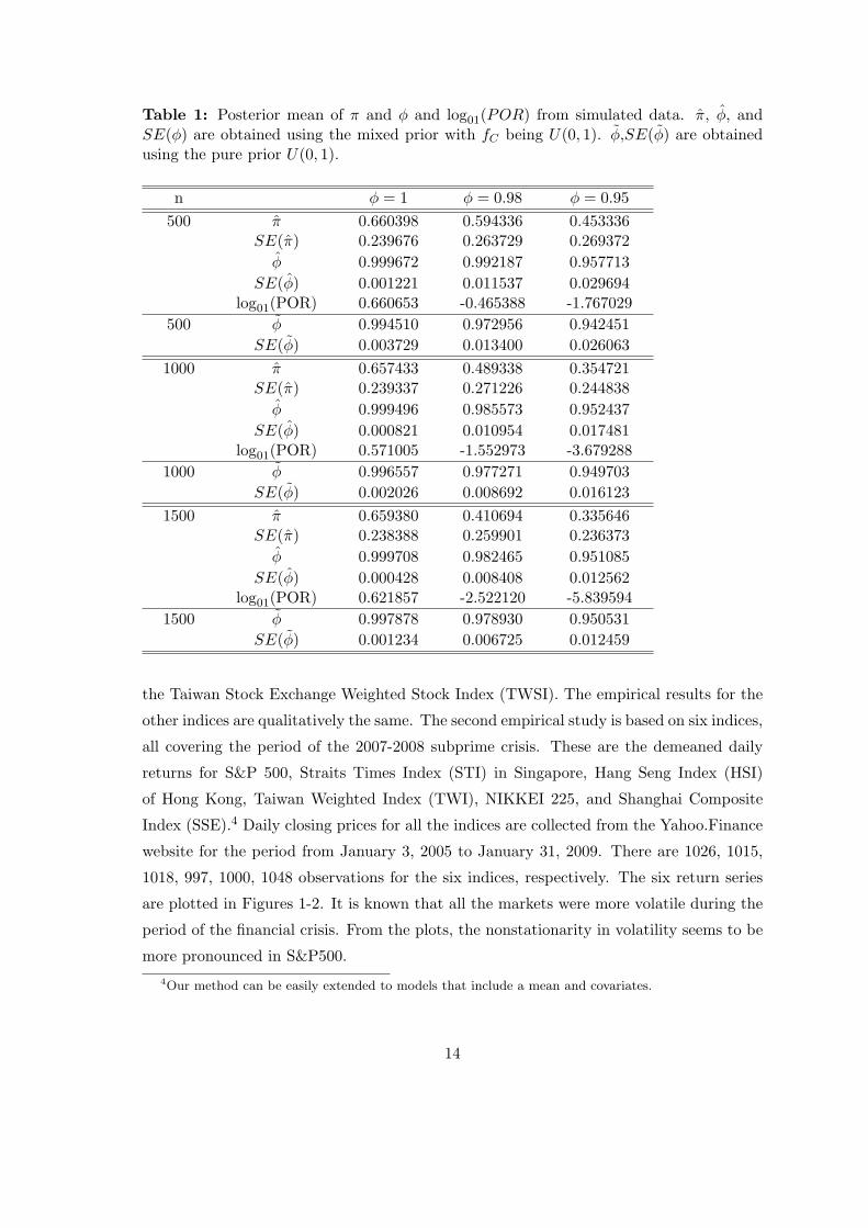
Table 1: Posterior mean of π and ϕ and log01(POR) from simulated data. π, ϕ, andSE(ϕ) are obtained using the mixed prior with fC being U(0, 1). ϕ,SE(ϕ) are obtainedusing the pure prior U(0, 1).
n ϕ = 1 ϕ = 0.98 ϕ = 0.95
500 π 0.660398 0.594336 0.453336SE(π) 0.239676 0.263729 0.269372
ϕ 0.999672 0.992187 0.957713
SE(ϕ) 0.001221 0.011537 0.029694log01(POR) 0.660653 -0.465388 -1.767029
500 ϕ 0.994510 0.972956 0.942451
SE(ϕ) 0.003729 0.013400 0.026063
1000 π 0.657433 0.489338 0.354721SE(π) 0.239337 0.271226 0.244838
ϕ 0.999496 0.985573 0.952437
SE(ϕ) 0.000821 0.010954 0.017481log01(POR) 0.571005 -1.552973 -3.679288
1000 ϕ 0.996557 0.977271 0.949703
SE(ϕ) 0.002026 0.008692 0.016123
1500 π 0.659380 0.410694 0.335646SE(π) 0.238388 0.259901 0.236373
ϕ 0.999708 0.982465 0.951085
SE(ϕ) 0.000428 0.008408 0.012562log01(POR) 0.621857 -2.522120 -5.839594
1500 ϕ 0.997878 0.978930 0.950531
SE(ϕ) 0.001234 0.006725 0.012459
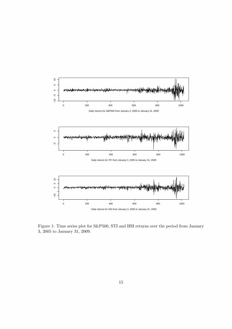
the Taiwan Stock Exchange Weighted Stock Index (TWSI). The empirical results for the
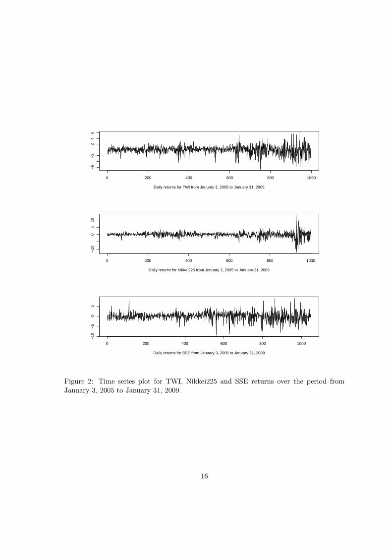
other indices are qualitatively the same. The second empirical study is based on six indices,
all covering the period of the 2007-2008 subprime crisis. These are the demeaned daily
returns for S&P 500, Straits Times Index (STI) in Singapore, Hang Seng Index (HSI)
of Hong Kong, Taiwan Weighted Index (TWI), NIKKEI 225, and Shanghai Composite
Index (SSE).4 Daily closing prices for all the indices are collected from the Yahoo.Finance
website for the period from January 3, 2005 to January 31, 2009. There are 1026, 1015,
1018, 997, 1000, 1048 observations for the six indices, respectively. The six return series
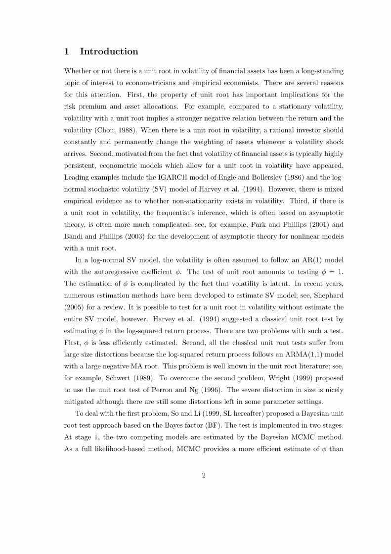
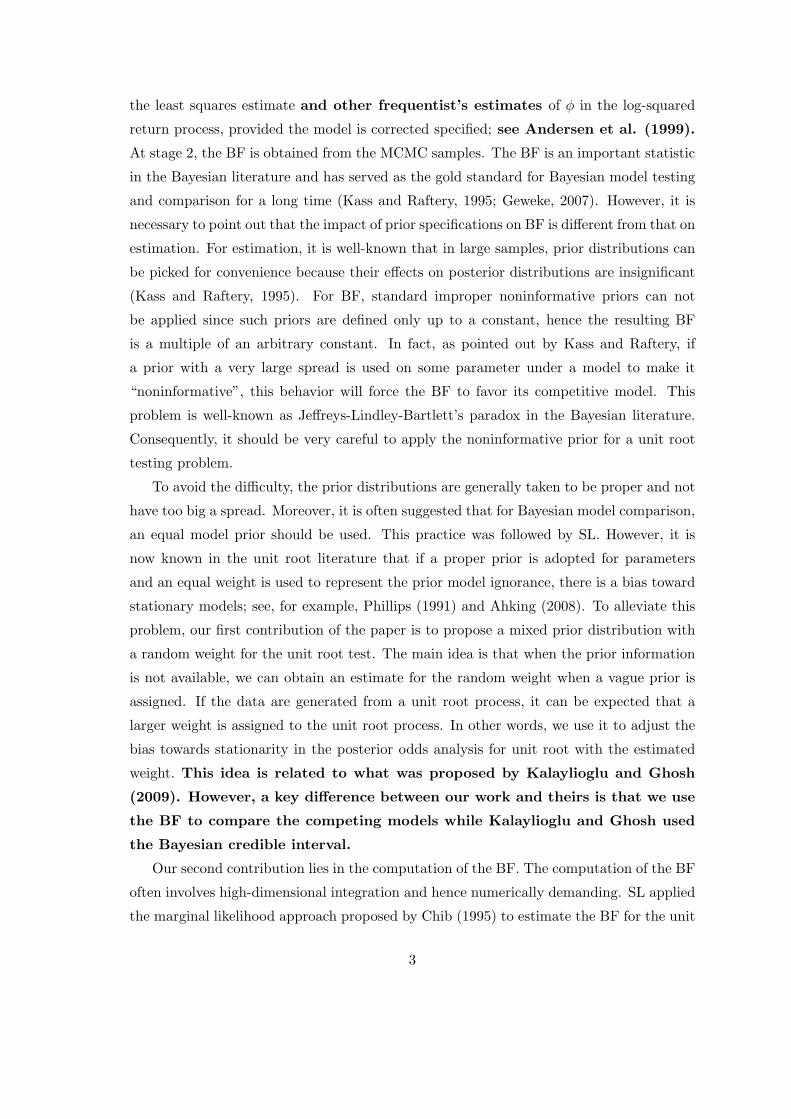
are plotted in Figures 1-2. It is known that all the markets were more volatile during the
period of the financial crisis. From the plots, the nonstationarity in volatility seems to be
more pronounced in S&P500.
4Our method can be easily extended to models that include a mean and covariates.
14
0 200 400 600 800 1000
−10
−5
05
10
Daily returns for S&P500 from January 3, 2005 to January 31, 2009
0 200 400 600 800 1000
−5
05
Daily returns for STI from January 3, 2005 to January 31, 2009
0 200 400 600 800 1000
−10
05
10
Daily returns for HSI from January 3, 2005 to January 31, 2009
Figure 1: Time series plot for S&P500, STI and HSI returns over the period from January3, 2005 to January 31, 2009.
15
0 200 400 600 800 1000
−6
−2
24
6
Daily returns for TWI from January 3, 2005 to January 31, 2009
0 200 400 600 800 1000
−10
05
10
Daily returns for Nikkei225 from January 3, 2005 to January 31, 2009
0 200 400 600 800 1000
−10
−5
05
Daily returns for SSE from January 3, 2005 to January 31, 2009
Figure 2: Time series plot for TWI, Nikkei225 and SSE returns over the period fromJanuary 3, 2005 to January 31, 2009.
16
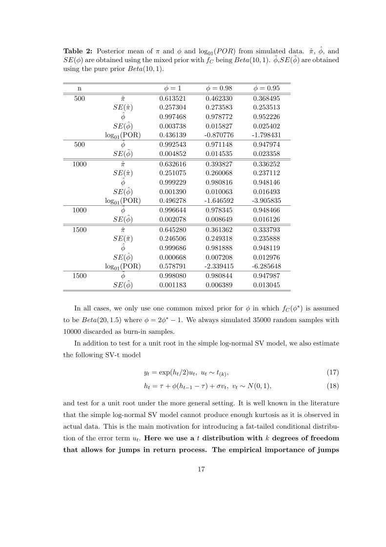
Table 2: Posterior mean of π and ϕ and log01(POR) from simulated data. π, ϕ, andSE(ϕ) are obtained using the mixed prior with fC being Beta(10, 1). ϕ,SE(ϕ) are obtainedusing the pure prior Beta(10, 1).
n ϕ = 1 ϕ = 0.98 ϕ = 0.95
500 π 0.613521 0.462330 0.368495SE(π) 0.257304 0.273583 0.253513
ϕ 0.997468 0.978772 0.952226
SE(ϕ) 0.003738 0.015827 0.025402log01(POR) 0.436139 -0.870776 -1.798431
500 ϕ 0.992543 0.971148 0.947974
SE(ϕ) 0.004852 0.014535 0.023358
1000 π 0.632616 0.393827 0.336252SE(π) 0.251075 0.260068 0.237112
ϕ 0.999229 0.980816 0.948146
SE(ϕ) 0.001390 0.010063 0.016493log01(POR) 0.496278 -1.646592 -3.905835
1000 ϕ 0.996644 0.978345 0.948466
SE(ϕ) 0.002078 0.008649 0.016126
1500 π 0.645280 0.361362 0.333793SE(π) 0.246506 0.249318 0.235888
ϕ 0.999686 0.981888 0.948119
SE(ϕ) 0.000668 0.007208 0.012976log01(POR) 0.578791 -2.339415 -6.285648
1500 ϕ 0.998080 0.980844 0.947987
SE(ϕ) 0.001183 0.006389 0.013045
In all cases, we only use one common mixed prior for ϕ in which fC(ϕ∗) is assumed
to be Beta(20, 1.5) where ϕ = 2ϕ∗ − 1. We always simulated 35000 random samples with
10000 discarded as burn-in samples.
In addition to test for a unit root in the simple log-normal SV model, we also estimate
the following SV-t model
yt = exp(ht/2)ut, ut ∼ t(k), (17)
ht = τ + ϕ(ht−1 − τ) + σvt, vt ∼ N(0, 1), (18)
and test for a unit root under the more general setting. It is well known in the literature
that the simple log-normal SV model cannot produce enough kurtosis as it is observed in
actual data. This is the main motivation for introducing a fat-tailed conditional distribu-
tion of the error term ut. Here we use a t distribution with k degrees of freedom
that allows for jumps in return process. The empirical importance of jumps
17

Table 3: Posterior mean of π and ϕ and log01(POR) from simulated data. π, ϕ, andSE(ϕ) are obtained using the mixed prior with fC being Beta(20, 2). ϕ,SE(ϕ) are obtainedusing the pure prior Beta(20, 2).
n ϕ = 1 ϕ = 0.98 ϕ = 0.95
500 π 0.637654 0.504941 0.376864SE(π) 0.247124 0.273527 0.253784
ϕ 0.997752 0.983746 0.947044
SE(ϕ) 0.003408 0.014309 0.025526log01(POR) 0.773400 -0.551413 -1.960837
500 ϕ 0.989874 0.972451 0.942477
SE(ϕ) 0.005208 0.012176 0.022994
1000 π 0.653888 0.425385 0.336909SE(π) 0.241840 0.264469 0.238225
ϕ 0.999518 0.981596 0.948867
SE(ϕ) 0.001055 0.010266 0.015704ˆlog01(POR) 0.954405 -1.579565 -3.945060
1000 ϕ 0.995418 0.976659 0.948180
SE(ϕ) 0.002178 0.008084 0.015282
1500 π 0.656273 0.366009 0.333473SE(π) 0.239154 0.249150 0.235813
ϕ 0.999561 0.979079 0.949505
SE(ϕ) 0.000560 0.007606 0.012501log01(POR) 0.999422 -2.668887 -6.001346
1500 ϕ 0.997143 0.977704 0.949588
SE(ϕ) 0.001303 0.006501 0.012410
was documented in a recent study by Li, et al. (2009). Relative to the normal
distribution, the t distribution will absorb some abnormal behavior in ht, as a result, we
expect that the volatility process, ht, is smoother, making the unit root model more dif-
ficult to reject. Following much of the literature, we rewrite the t distribution with a
normal scale mixture representation, namely,
ut|wt ∼ N(0, w−1t ), wt ∼ Γ(k/2, k/2).
It is easy to show that for the SV-t model, the BF has the same expression as in (15).
Table 5 report the posterior mean of ϕ, π, log01(BF) and log01(POR) for TWSI used by
SL. The empirical results based on the simple log-normal SV model suggest that although
the posterior mean of ϕ is so close to unity and the estimate of π is large than 0.5, we still
reject the unit root hypothesis. The marginal likelihood of the estimated stationary model
is so much larger than that of the estimated unit root model so that the adjustment from
18
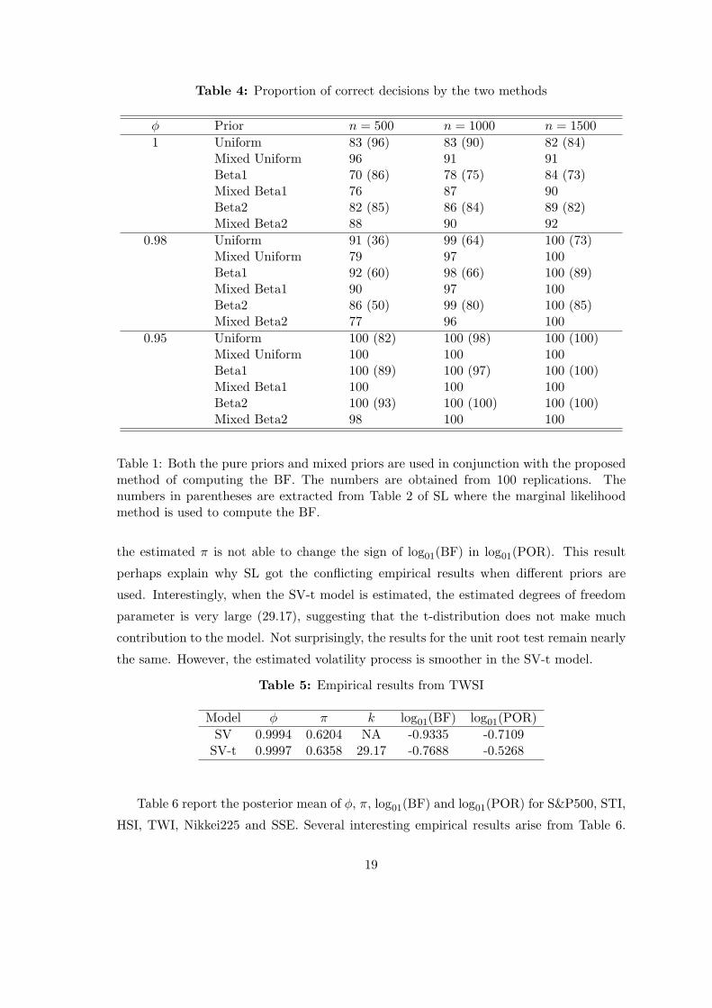
Table 4: Proportion of correct decisions by the two methods
ϕ Prior n = 500 n = 1000 n = 1500
1 Uniform 83 (96) 83 (90) 82 (84)Mixed Uniform 96 91 91Beta1 70 (86) 78 (75) 84 (73)Mixed Beta1 76 87 90Beta2 82 (85) 86 (84) 89 (82)Mixed Beta2 88 90 92
0.98 Uniform 91 (36) 99 (64) 100 (73)Mixed Uniform 79 97 100Beta1 92 (60) 98 (66) 100 (89)Mixed Beta1 90 97 100Beta2 86 (50) 99 (80) 100 (85)Mixed Beta2 77 96 100
0.95 Uniform 100 (82) 100 (98) 100 (100)Mixed Uniform 100 100 100Beta1 100 (89) 100 (97) 100 (100)Mixed Beta1 100 100 100Beta2 100 (93) 100 (100) 100 (100)Mixed Beta2 98 100 100
Table 1: Both the pure priors and mixed priors are used in conjunction with the proposedmethod of computing the BF. The numbers are obtained from 100 replications. Thenumbers in parentheses are extracted from Table 2 of SL where the marginal likelihoodmethod is used to compute the BF.
the estimated π is not able to change the sign of log01(BF) in log01(POR). This result
perhaps explain why SL got the conflicting empirical results when different priors are
used. Interestingly, when the SV-t model is estimated, the estimated degrees of freedom
parameter is very large (29.17), suggesting that the t-distribution does not make much
contribution to the model. Not surprisingly, the results for the unit root test remain nearly
the same. However, the estimated volatility process is smoother in the SV-t model.
Table 5: Empirical results from TWSI
Model ϕ π k log01(BF) log01(POR)
SV 0.9994 0.6204 NA -0.9335 -0.7109SV-t 0.9997 0.6358 29.17 -0.7688 -0.5268
Table 6 report the posterior mean of ϕ, π, log01(BF) and log01(POR) for S&P500, STI,
HSI, TWI, Nikkei225 and SSE. Several interesting empirical results arise from Table 6.
19
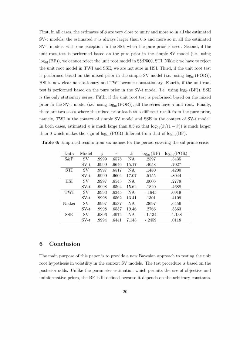
First, in all cases, the estimates of ϕ are very close to unity and more so in all the estimated
SV-t models; the estimated π is always larger than 0.5 and more so in all the estimated
SV-t models, with one exception in the SSE when the pure prior is used. Second, if the
unit root test is performed based on the pure prior in the simple SV model (i.e. using
log01(BF)), we cannot reject the unit root model in S&P500, STI, Nikkei; we have to reject
the unit root model in TWI and SSE; we are not sure in HSI. Third, if the unit root test
is performed based on the mixed prior in the simple SV model (i.e. using log01(POR)),
HSI is now clear nonstationary and TWI become nonstationary. Fourth, if the unit root
test is performed based on the pure prior in the SV-t model (i.e. using log01(BF)), SSE
is the only stationary series. Fifth, if the unit root test is performed based on the mixed
prior in the SV-t model (i.e. using log01(POR)), all the series have a unit root. Finally,
there are two cases where the mixed prior leads to a different result from the pure prior,
namely, TWI in the context of simple SV model and SSE in the context of SV-t model.
In both cases, estimated π is much large than 0.5 so that log01(π/(1− π)) is much larger
than 0 which makes the sign of log01(POR) different from that of log01(BF).
Table 6: Empirical results from six indices for the period covering the subprime crisis
Data Model ϕ π k log01(BF) log01(POR)
S&P SV .9999 .6578 NA .2597 .5435SV-t .9999 .6646 15.17 .4058 .7027
STI SV .9997 .6517 NA .1480 .4200SV-t .9999 .6604 17.07 .5155 .8044
HSI SV .9997 .6545 NA .0006 .2779SV-t .9998 .6594 15.62 .1820 .4688
TWI SV .9993 .6345 NA -.1645 .0919SV-t .9998 .6562 13.41 .1301 .4109
Nikkei SV .9997 .6537 NA .3697 .6456SV-t .9998 .6557 19.46 .2766 .5563
SSE SV .9896 .4974 NA -1.134 -1.138SV-t .9994 .6441 7.148 -.2459 .0118
6 Conclusion
The main purpose of this paper is to provide a new Bayesian approach to testing the unit
root hypothesis in volatility in the context SV models. The test procedure is based on the
posterior odds. Unlike the parameter estimation which permits the use of objective and
uninformative priors, the BF is ill-defined because it depends on the arbitrary constants.
20
As a result, an informative prior has to be used in order to do the posterior odds analysis.
To overcome this difficulty, one simple method suggested in Kass and Raftery (1995)
is to use part of the data as a training sample which is combined with the noninformative
prior distribution to produce an informative prior distribution. The BF is then computed
from the remainder of the data. However, the selection of the training sample may be
arbitrary. Other empirical measures, such as intrinsic BF of Berger and Pericchi (1996)
and fractional BF of O’Hagan (1995), also involve with theoretical or practical problems.
To the best of our knowledge, there is no satisfactory method to solve this Jeffreys-Lindley-
Bartlett’s paradox. In this paper, we propose to use a mixed informative prior distribution
with a random weight for the Bayesian unit root testing. The new method for computing
the BF is numerically stable and easy to implement. We illustrate the method using both
simulated data and real data. Simulations show that our method improve the performance
of the unit root test of So and Li (1999) in terms of both the “size” and the “power”.
Empirical analysis, based the equity data over the period covering the subprime crisis,
shows that the unit root hypothesis is not rejected when our method is used in the context
of the SV-t model.
Although our test suggests that the stationary AR model in volatility is inferior to the
unit root model, no mean the unit root model is the only way to produce high persistency
in volatility. Other models, which can potentially explain high persistency in volatility,
include the fractionally integrated SV models and the SV model with a shift in mean
and/or a shift in persistency. Although we do not pursuit this direction of research here,
our method can be adopted and modified to compare some of these alternative models.
There are two issues that warrant further investigation. First, BF is im-
portant for hypothesis testing and model selection. Kass and Raftery (1995)
gave rule-of-thumb critical values for BF for model compassion. In this paper,
we have used the critical value of 1 for making decisions. This means that we
simply choose the model with a larger marginal likelihood value. However, we
acknowledge that how to determine good critical values for BF is not trivial.
In fact, it can be easily shown that BF is a complex function of the observed
data, say, f(y). If the distribution of f(y) is known, the percentiles of the
distribution can be conveniently regarded as critical values. Unfortunately, in
most cases, the distribution of f(y) is not known. In this case, one can use a
simulation-based approach to obtain the distribution of f(y) and, hence, the
percentiles; see, for example, Vlachoes and Gelfand (2003). A natural choice
is to use a bootstrap method to obtain the distribution of f(y). However,
21
the implementation of the bootstrap method requires repetitive calculations
of BF and is usually time-consuming, especially for latent variable models.
Second, in general, Bayesian hypothesis testing is based on the assumption
that the model is correctly specified. If the model is misspecified, to the best
of our knowledge, there is no general result available on the impact of mis-
specification on the test. In the context of linear regression models, however,
a contribution was recently made by Muller (2011).
References
Ahking, F,W. (2004). The Power of the “Objective” Bayesian Unit-Root Test. Working
papers, University of Connecticut, Department of Economics.
Aitkin,M. (1991). Posterior Bayes factor (with discussion). Journal of the Royal Statis-
tical Society. Series B, 53(1), 111-142.
Andersen, T., Chung, H., Sorensen, R. (1999). Efficient method of moments
estimation of a stochastic volatility model: A Monte Carlo study. Journal
of Econometrics, 91, 61-87.
Bandi, F.M. and Phillips, P.C.B. (2003). Fully Nonparametric Estimation of Scalar
Diffusion Models. Econometrica, 71(1), 241-83.
Berg, A., Meyer, R., and Yu, J. (2004). Deviance information criterion for comparing
stochastic volatility models. Journal of Business and Economic Statistics, 22, 107-
120.
Berger, J.O. and Bernardo, J.M. (1992). On the development of reference prior method.
In J.M. Bernardo, J.O. Berger, A.P. Dawid, and A.F.M. Smith. Bayesian Statistics,
vol 4, pp.35-60. Oxford University Press,Oxford.
Berger, J.O. and Pericchi, L.R. (1996). The intrinsic Bayes factor for model selection
and prediction. Journal of the American Statistical Association, 91, 109-122.
Chen, M.H., Shao, Q.M. and Ibrahim, J.G. (2000). Monte Carlo Methods in
Bayesian Computation. Springer, New York.
Chib, S. (1995) Marginal likelihood from the Gibbs output. Journal of the American
Statistical Association, 90, 1313-1321.
22
Chib, S., Nardari, F. and Shephard, N. (2002). Markov chain Monte Carlo methods for
stochastic volatility models. Journal of Econometrics, 108, 281-316.
Chou, R.Y. (1988). Volatility Persistency and stock valuation: some empirical evidence
using GARCH. Journal of Applied Econometrics, 3, 279-294.
Engle, R.F. and Bollerslev, T. (1986). Modeling the persistence of conditional variances.
Econometric Reviews, 5, 1-50.
Geweke, J. (2007). Bayesian model comparison and validation. American Economic
Review, 97(2), 60-64.
Harvey, A.C., Ruiz, E. and Shephard, N. (1994). Multivariate stochastic variance models.
Review of Economic Studies, 61 , 247–264.
Huang, J. and L. Xu (2009), Stochastic Volatility Models for Asset Returns with Jumps,
Leverage Effect and Heavy-Tails: A Specification Analysis Based on MCMC, working
paper.
Jacquier, E., Polson, N. G. and Rossi, P. E. (2004). Bayesian analysis of stochastic
variance models with fat-tails and correlated errors. Journal of Econometrics, 12,
371-389.
Jeffreys, H. (1961). Theory of Probability. Clarendon Press,Oxford.
Kalaylioglu, Z. I. and Ghosh, S. K. (2009). Bayesian unit root tests for
stochastic volatility models. Statistical Methodology, 6, 189-201.
Kass, R. E. and Raftery, A. E. (1995). Bayes Factor. Journal of the Americana Statistical
Association, 90, 773-795.
Kim, S., Shephard, N. and Chib, S. (1998). Stochastic volatility: likelihood inference
and comparison with ARCH models. Review of Economic Statistics, 12, 361-393.
Kou, S.C., Xie, X.S. and Liu, J.S. (2005). Bayesian analysis of single-molecule
experiments. Applied Statistics, 54(3), 1-28.
Li, H., Wells, M., and Yu, C. (2009). A Bayesian Analysis of Return Dynam-
ics with Levy Jumps. Review of Financial Studies 21, 2345-2378.
Meyer, R. and Yu, J. (2000). BUGS for a Bayesian analysis of stochastic volatility
models. Econometrics Journal, 3, 198-215.
23
Muller, U.K. (2011). Risk of Bayesian inference in misspecified models, and sandwich
covariance matrix. Working paper.
Nicolae, D., Meng, X.L., and Kong, A. (2008). Quantifying the Fraction
of Missing Information for Hypothesis Testing in Statistical and Genetic
Studies. Statistical Science, 23, 287-331.
O’Hagan, A. (1995). Fractional Bayes factor of model comparison (with discussion).
Journal of Royal Statistical Society, Series, B, 57, 99-138.
Park, J.Y. and Phillips, P.C.B. (2001), Nonlinear regressions with integrated time series.
Econometrica, 69, 117-161.
Perron, P. and Ng, S. (1996). Useful Modifications to some Unit Root Tests with De-
pendent Errors and their Local Asymptotic Properties. The Review of Economic
Studies, 63, 435-463.
Phillips, P.C.B. (1991). Bayesian routes and unit roots: De rebus prioribus semper est
disputandum. Journal of Applied Econometrics, 6, 435-474.
Robert, C.P. (2001). The Bayesian choice. Springer, second edition.
Schotman, P. and van Dijk, H.K. (1991). A Bayesian analysis of the unit root in real
exchange rates. Journal of Econometrics, 49(1-2), 195-238.
Schwert, G.W. (1989). Tests for Unit Roots: A Monte Carlo Investigation. Journal of
Business and Economic Statistics, 7(2), 147-59.
Shephard, N. (2005). Stochastic Volatility: Selected Readings. Oxford: Oxford University
Press.
Sims, C.A. (1988). Bayesian skepticism on unit root econometrics. Journal of Economic
Dynamics and Control, 12, 463-464.
So, M.K.P. and Li, W.K. (1999). Bayesian unit-root testing in stochastic volatility mod-
els. Journal of Business and Economic Statistics, 17(4),491-496.
Sturtz, S, Ligges, U, Gelman, A. (2005). R2WinBUGS: A Package for Running Win-
BUGS from R. Journal of Statistical Software 12(3), 1-16.
Tanner, T.A. and Wong, W.H. (1996). The calculation of posterior distributions by data
augmentation. Journal of the American Statistical Association, 82, 528-549.
24

Vlachos, P.K. and Gelfand, A.E. (2003). On the calibration of Bayesian
model choice criteria. Journal of Statistical Planning and Inference, 111,
223-234.
Wright, J.H. (1999). Testing for a Unit Root in the Volatility of Asset Returns. Journal
of Applied Econometrics, 14(3), 309-18.
Yu, J. (2005). On leverage effect on stochastic volatility models. Journal of Econometrics,
127(2), 165-178.
Yu, J., and Meyer, R. (2006). Multivariate Stochastic Volatility Models: Bayesian Esti-
mation and Model Comparison. Econometric Reviews, 25, 361-384.
25


![Bayesian Techniques for Discrete Stochastic …Markov chain Monte Carlo (MCMC) methods for stochastic volatility (SV) models [139] and the availability of more or less standardized](https://img.pdfslide.us/doc/110x75/5f70bf2e87d6a31cac180ea2/bayesian-techniques-for-discrete-stochastic-markov-chain-monte-carlo-mcmc-methods.jpg)