A New Approach to Modelling Sector Stock Returns in China · A New Approach to Modelling Sector Stock Returns in China Chong, Terence Tai Leung and Li, Nasha and Zou, Lin The Chinese

Munich Personal RePEc Archive

A New Approach to Modelling Sector

Stock Returns in China

Chong, Terence Tai Leung and Li, Nasha and Zou, Lin

The Chinese University of Hong Kong, The Chinese University of

Hong Kong, A New Approach to Modelling Sector Stock Returns in

China

1 September 2016

Online at https://mpra.ub.uni-muenchen.de/80554/

MPRA Paper No. 80554, posted 02 Aug 2017 14:50 UTC

1

A New Approach to Modelling Sector Stock Returns in China

Terence Tai-Leung Chong

Nasha Li

Department of Economics

The Chinese University of Hong Kong

Lin Zou

Asset Allocation & Strategic Research Department

China Investment Corporation

1/9/2016

Abstract: This paper analyzes the relationship between excess stock returns and the

macroeconomy of China. A factor-augmented regression is applied to a panel of 123

monthly Chinese macroeconomic time series. Eight fundamental macroeconomic

factors are identified and used to examine the excess returns in industrial, commercial,

real estate and utilities sectors of the market. It is found that interest rate, output level,

as well as property supply factors possess explanatory power for sector stock returns

in China.

JEL Classification: C22, G1

Keywords: Factor-augmented regression; Excess stock returns; Common factors.

Address corresponding to: Terence Tai-Leung Chong, Department of Economics, The Chinese

University of Hong Kong, Shatin, N.T., Hong Kong. E-mail: [email protected]. Phone no.

852-3948193. Homepage: http://www.cuhk.edu.hk/eco/staff/tlchong/tlchong3.htm

2

INTRODUCTION

Macroeconomic variables are considered important in predicting stock returns.

However, most empirical studies on the impact of macroeconomic fundamentals on

equity returns focus only on a small set of predictors (Chen et al., 1986; Reilly and

Brown, 2000; Goyal and Welch, 2008). Chen et al. (1986) find that interest rates,

expected and unexpected inflation and industrial production are priced significantly.

Hamao (1988) investigates the Japanese stock market and obtains similar results.

Chen (1991) finds that the market excess return is negatively correlated with T-bill

rates and lagged production growth rates, but positively correlated to expected future

economic growth. Other variables that might be relevant are the risk-free rate of

return (Ang and Bekaert, 2007), money supply (Jensen et al., 1996), and consumption

and investment (Lettau and Ludvigson, 2001). Lamont (2000) finds that investment

plans can also be used to forecast stock returns. However, previous models containing

macroeconomic variables have been criticized for producing contradictory results. For

example, Shanken and Weinstein (1990) find that the statistical importance of macro

factors for equity returns has been discounted after the standard errors of estimates in

Chen et al. (1986) were revised. Goyal and Welch (2008) find that the in-sample and

out-of-sample performance of these predictors are unstable after revisiting the

performance of traditional predictors of equity premiums. Recent studies in this area

include Goh et al. (2013), Liang and Willett (2015) and Chen and Chiang (2016).

An explanation for the poor performance of the aforementioned variables is that they

fail to capture time-varying economic conditions (Bai, 2010). Investors are exposed to

a complex macroeconomic environment, where a vast number of economic factors

can affect market behavior and stock prices. Previous studies only partially capture

these economic factors due to the limited number of macro variables used. In this

paper, we use a large panel of macroeconomic data to explain the equity premium in

China. To avoid the dimensionality problem, we adopt factor analysis – used in

several recent studies – to summarize the information of the variables. Stock and

Watson (2002a) use principal component analysis (herein referred to as PCA) to

estimate common factors from the predictors and to evaluate the relationship between

common factors and the variable forecasted by linear regression. It is found that this

forecasting model outperforms conventional models when using a small number of

3

variables as independent variables. Stock and Watson (2002b) show that the common

factors obtained from the PCA consistently span the information space of the panel

data of the independent variables. Bernanke et al. (2005) propose a factor-augmented

vector autoregressive (FAVAR) approach, which incorporates the common factors

derived from macroeconomic series into the traditional structural VAR model to

estimate the effects of a monetary policy. It is found that FAVAR can properly identify

the mechanism of monetary transmission. Ludvigson and Ng (2007) apply the factor

model to test the risk-return relationship in the stock market. Ludvigson and Ng (2009)

compare the common factors estimated from the principal component method and

Gibbs sampling. It is shown that macroeconomic factors have statistically significant

explanatory power over excess bond returns.

This paper is the first work that applies the factor-augmented regression model to

explain excess stock returns in China. We contribute to the existing literature by

addressing two questions. Firstly, can the factors extracted from numerous data be

used to predict the equity excess returns in the China stock market? And secondly, do

these factors provide extra information after controlling for predetermined predictive

variables? Following Stock and Watson (2002a) and Ludvigson and Ng (2007, 2009),

the common factors from a large number of macroeconomic time series are used as

independent variables to explain excess stock returns. The estimation results suggest

that the macroeconomic factors contain important information on the stock market

that is not captured by traditionally selected predictor variables. Information related to

output level, interest rate, and property supply can help improve the predictability of

excess returns. In general, macroeconomic factors are able to explain most sectors

except for the commercial sector in China.1

The rest of this paper is organized as follows. Section 2 presents the model and

provides economic interpretations of the factors extracted. Section 3 describes the

data. Section 4 reports the empirical results for the one-month-ahead predictive

relationship. Section 5 concludes the paper.

FACTOR-AUGMENTED REGRESSION

The Factor Approach to Assess the Excess Equity Returns

A standard approach to assessing the predictability of excess equity returns, rxt+1, is to

4

select a set of K observed variables at time t, given by a 1K vector tZ , and

estimate the model

'

1 1t t trx Z . (2)

where 1 1t t trx r y , for 1,...,t T denotes the aggregate excess returns on the

stock market over time; 1tr is the return of the stock market from time t to time

1t , and ty is the risk-free rate at time t.

tZ

could include fundamentals, such as

the three Fama-French factors, term spread, credit spread, and the dividend-price ratio

(e.g., Fama and French, 1988). The above model can be extended to

' '

1 1t t t trx x Z

. (3)

where xt is a vector of macroeconomic variables, such as interest rate, inflation, and

industrial production (e.g., Chen et al., 1986). However, the inclusion of all candidate

macroeconomic predictors in a linear regression is technically infeasible. For example,

suppose we observe a T N panel of macroeconomic data with elements

'

1 2( , ,..., )t t t Nt

x x x x , t = 1,…, T. There would be 2N combinations to be considered

as the set of candidate predictors. Moreover, as the dimension of tx increases, the

regression quickly runs into the degrees-of-freedom problem, and the estimation

cannot be done when N K T .

To address the problem, we employ the factor approach to model the variations of a

large number of variables by a relatively few number of common factors. Suppose itx

can be represented by r common latent factors ft,

'

it i t itx f e (4)

where i is a r×1 vector of corresponding latent factor loadings, and ite is the

idiosyncratic error2. For example, if itx

measures the return of asset i in period t,

5

tf could be a vector of systematic risk, i will be the exposure to the risk factors,

and itx will be the idiosyncratic returns.

If these factors are observed, we can then replace Equation (3) by the following

factor-augmented regression

' '

1 1t t t trx F Z , (5)

where Ft can be ft or a subset of ft and its dimension is much smaller than that of tx

(r<<N), yet has good explanatory power of 1trx . Equation (2) is nested within the

factor-augmented regression equation (5). Through equation (5), we can test the

importance of itx via tF , even in the presence of tZ . In our study, tZ represents

the fundamental features, which contain the three Fama-French factors: market

premium, SMB (small [market capitalization] minus big), and HML (high

[book-to-market ratio] minus low).

Note that the common factorstf cannot be observed and need to be estimated from

data tx .

Estimation of Latent Factors (ft)

As defined previously, N is the number of cross-sectional units and T is the

number of time series observations. For 1,2,...,i N , 1,...,t T , a factor model

defined in equation (4) can be estimated by principal components analysis. Since the

common factors ft is not observed, will be estimated, and spans the same space as

ft when N, T →∞. Bai and Ng (2006) show that if 0T N as ,N T , the

sampling uncertainty from such estimation is negligible. Bai and Ng (2002) develop

the panel information criteria, IC2 criteria, to determine the optimal number of factors.

We first follow the method of Bai and Ng (2002) to search for the optimal number of

common factors. We then use the method in Connor and Korajzcyk (1986) to estimate

ft. According to Stock and Watson (2002a), the PCA can obtain a consistent estimate

6

of the information space, and is computationally straightforward compared to other

methods.

Since ft and λi cannot be separately identified, only a r×r factor matrix will be

identified. Let Ʌ ≡ ,… , ′. The T r estimated matrix ˆtf is T times the

r eigenvectors corresponding to the r largest eigenvalues of the T T matrix

' ( )xx TN in descending order, with the constraint / . Ir is an r-dimensional

identity matrix, and normalization can help obtain ' ˆˆ x f T . Intuitively, for time t ,

ˆtf is a linear combination of the N macro variables '

1 2( , ,..., )t t t Nt

x x x x . The linear

combination is chosen optimally to minimize the sum of squared residuals Ʌ .

DATA

The macroeconomic dataset used to estimate the principal components is a

balanced panel of 123 monthly series for 117 months, running from January 2000 to

September 2009. The entirety of the series is transformed for stationarity and

standardized for estimation purposes, applying for seasonal adjustments whenever

necessary. The dataset is drawn from CEIC Macroeconomic Databases for Emerging

and Developed Markets (CEIC). We use the data from GTA Research Service Center

(GTA) to construct a broad market profile in order to calculate the three Fama-French

factors for the Chinese stock market, with a focus on non-financial stocks.3 IPO

month returns can be problematic since many of the individual stocks have severe

price jumps during IPO month. We thus exclude the first-month return data of

individual stocks. Some listed companies experience negative book value of equity, so

we exclude these companies after their book values turn negative.4 We also exclude

stocks that cease trading for more than three months after listing. A total of 1719

stocks is included in our construction of a value-weighted portfolio. We only use

tradable shares to compute the market capitalization for all the companies.

All listed stocks are sorted according to two dimensions. The first dimension is the

market capitalization (i.e., based on tradable shares) divided into two groups with an

equal number of stocks – the small cap group (S) and the big cap group (B). The

7

second dimension is defined by the book-to-market ratio, with the highest ranked 30%

of stocks based on this ratio categorized as “high book-to-market” (H), the following

40% as “medium book-to-market” (M), and the last 30% as “low book-to-market” (L).

As a result, six portfolios are formed from the intersection of the two size and three

book-to-market ratio groups. All stocks are placed into the six categories and defined

by two dimensions: small/high, small/medium, small/low, big/high, big/medium,

big/low.

The predetermined independent variables are the Fama-French factors of SMB and

HML, which are derived in a way similar to that of Fama and French (1992) and

Wang and Xu (2004). We define a SMB variable, which is calculated as the difference

between the average return of the three small-cap portfolios (small/low, small/medium,

and small/high) and the average return of the three big-cap portfolios (big/low,

big/medium, and big/high), i.e.,

/ / / / / /

3 3

S L S M S H B L B M B HSMB

where /S L is the return of the group of small size and low book-to-market ratio,

/S M is the return of the group of small size and medium book-to-market ratio, and

/S H is the return of the group of small size and high book-to-market ratio, etc.

SMB measures the excess returns of small caps over big caps. We also define an HML

variable, which is the difference between the average return of the two high

book-to-market ratio portfolios (small/high, and big/high) and the average return of

two low book-to-market ratio portfolios (small/low and big/low), i.e.,

/ / / /

2 2

S H B H S L B LHML

,

HML measures the excess returns of value stocks over growth stocks.

8

Furthermore, market premium (i.e., the excess returns of the market portfolio) is

included in the investigation of sector index excess returns. Two types of excess

returns are considered in our study as dependent variables: market return and index

return. Excess market return, or monthly returns of the portfolio minus the monthly

risk-free rate, is derived from the constructed broad market (i.e., non-financial)

portfolios. Excess index return, or the monthly index returns minus the monthly

risk-free rate, is derived from sector indices, which include the industrial index,

commercial index, real estate index, and utilities index. The monthly risk-free rate is

the one-year lump-sum deposit and withdrawal time deposit interest rate, which we

obtain from GTA.

EMPIRICAL RESULTS

Common Factors

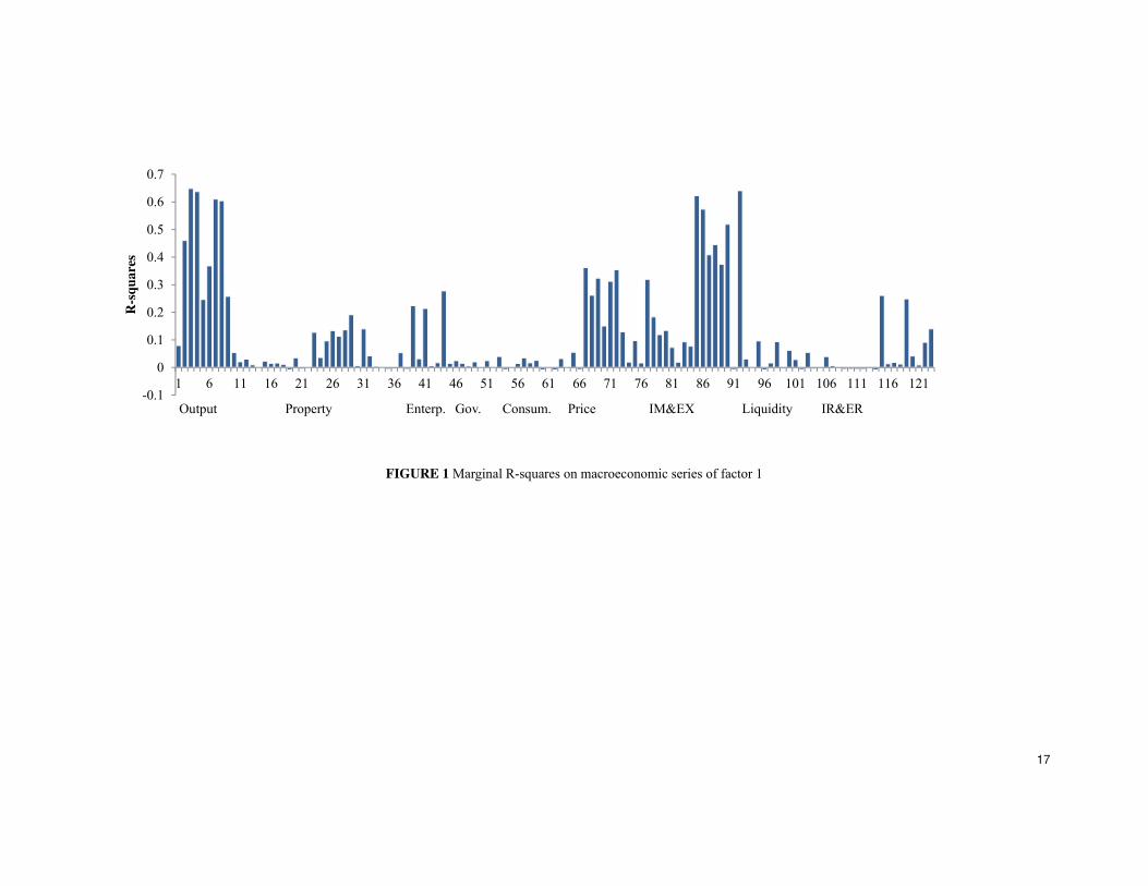
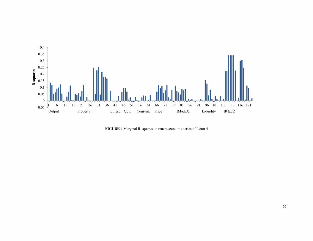
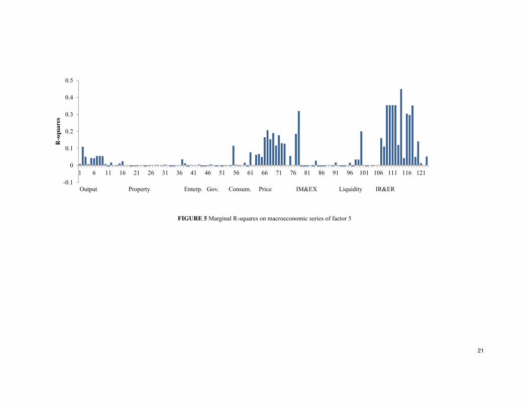
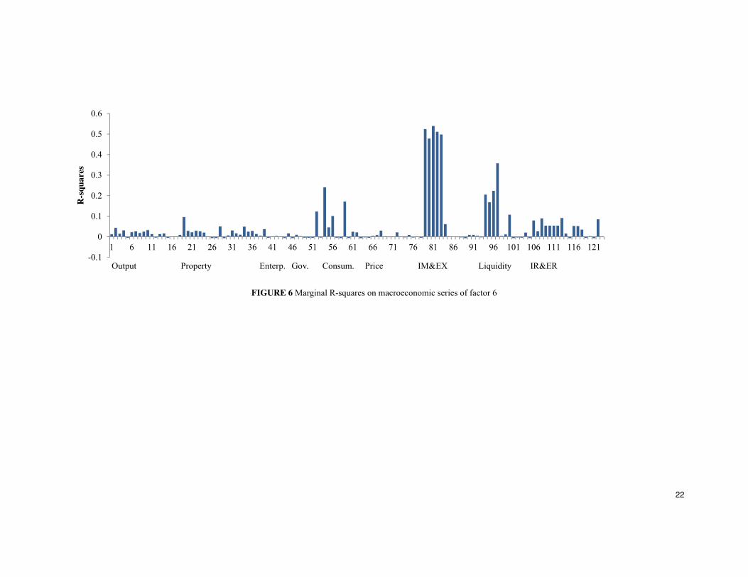
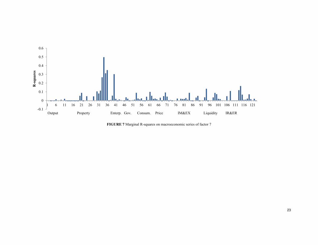
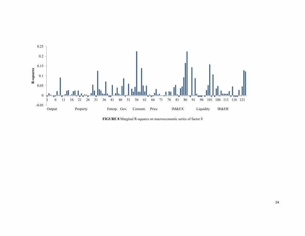
The factors are explained based on their marginal 2R . We utilize the eight common

factors stipulated in Bai and Ng’s (2002) 2IC criteria of and regress each series in the

macroeconomic dataset to obtain their marginal adjusted 2R and coefficients. The

marginal adjusted 2R indicates how closely each factor is moving with each data

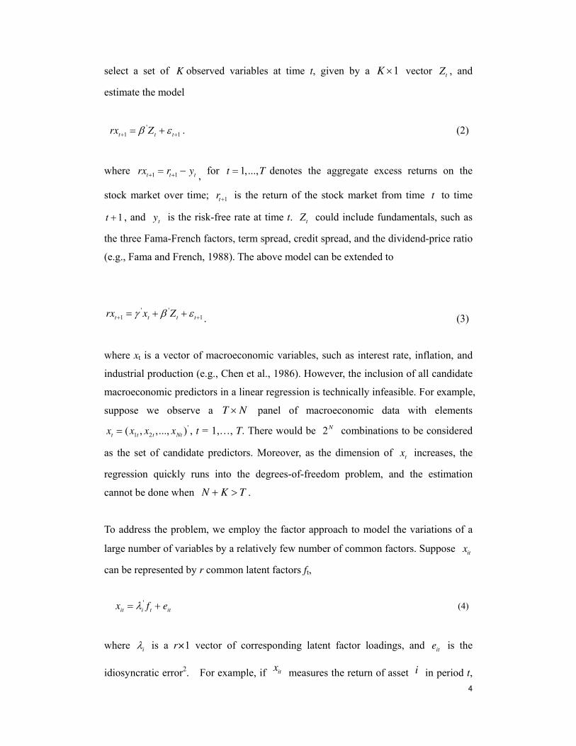
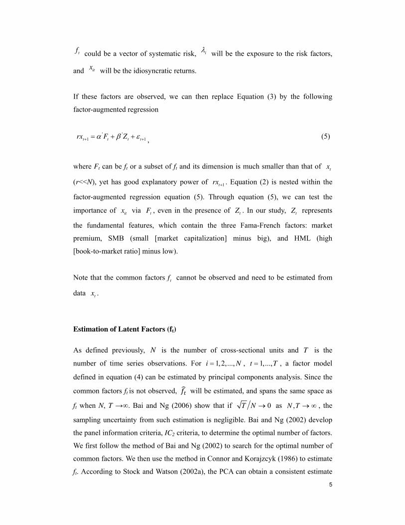
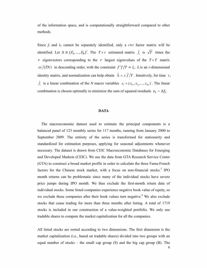
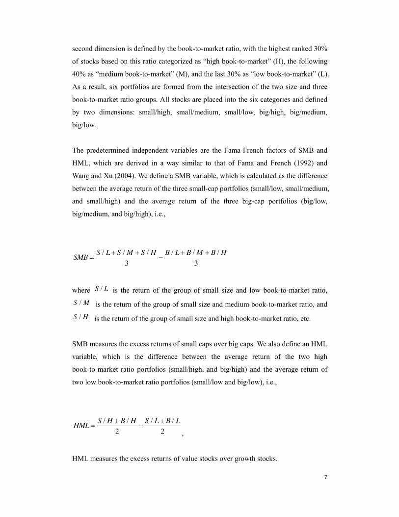
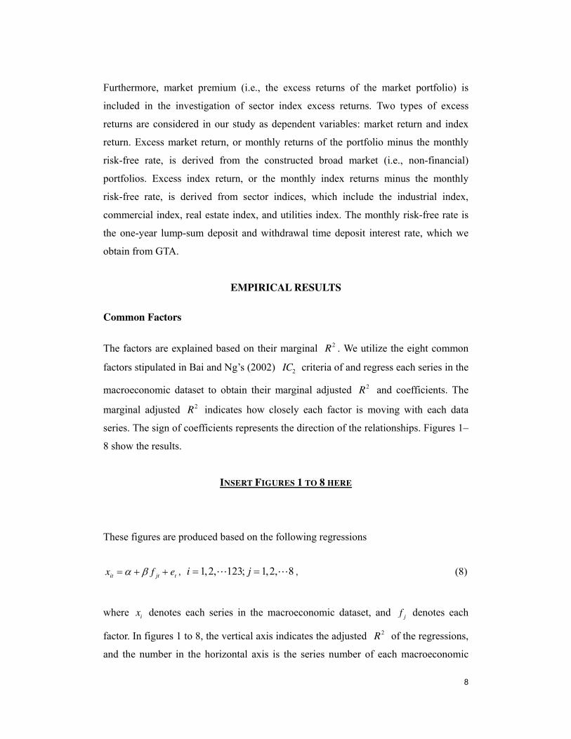
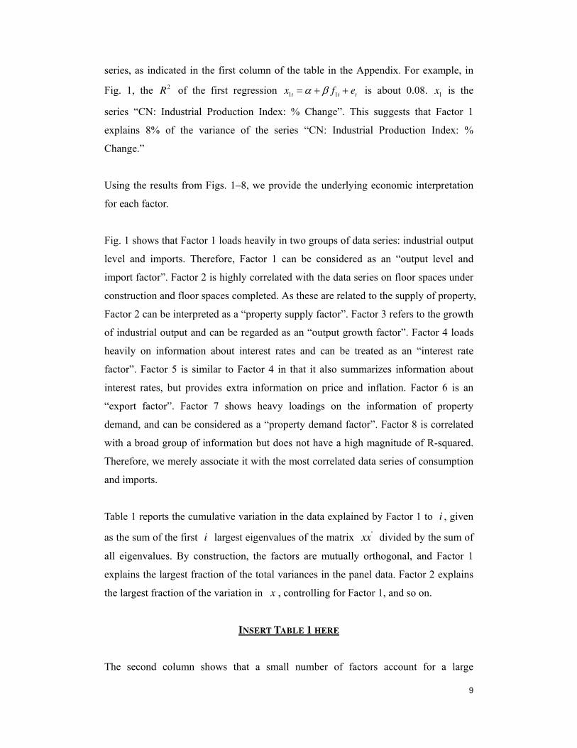
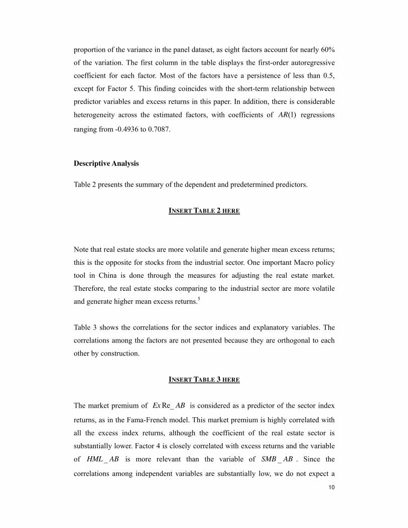
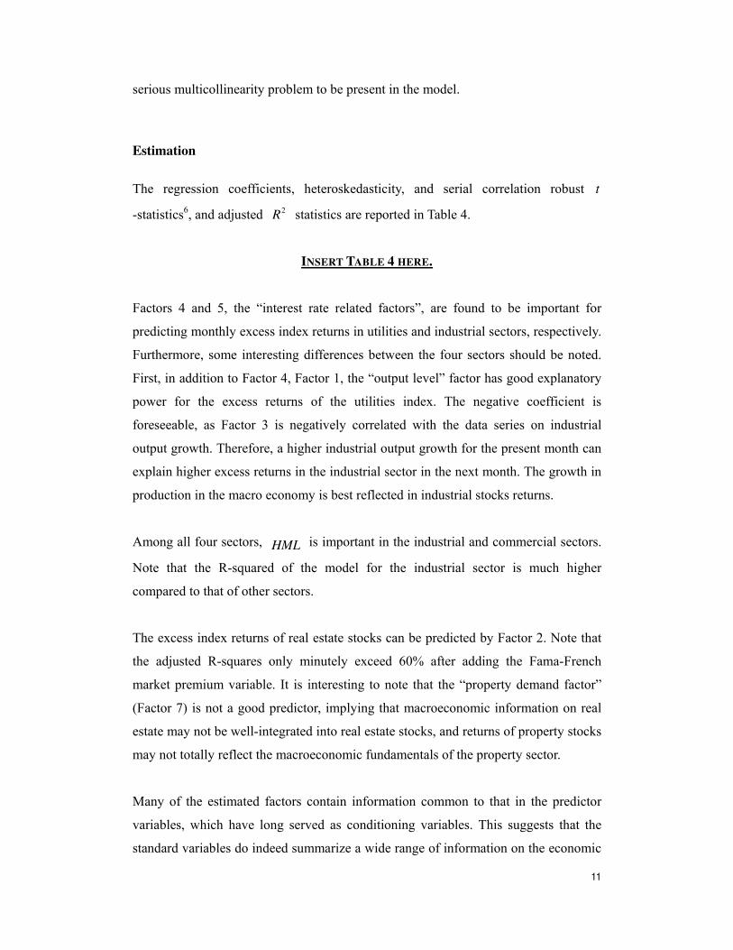
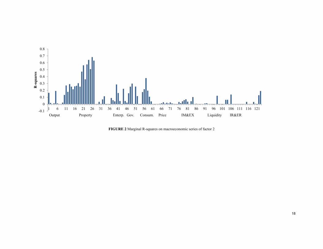
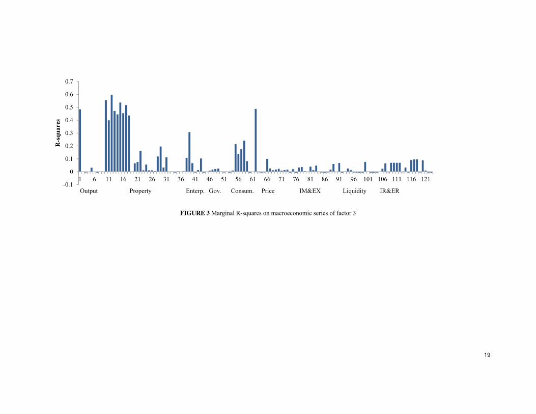
series. The sign of coefficients represents the direction of the relationships. Figures 1–

8 show the results.

INSERT FIGURES 1 TO 8 HERE

These figures are produced based on the following regressions

it jt tx f e , 1,2, 123; 1,2, 8i j , (8)

where ix denotes each series in the macroeconomic dataset, and j

f denotes each

factor. In figures 1 to 8, the vertical axis indicates the adjusted 2R of the regressions,

and the number in the horizontal axis is the series number of each macroeconomic

9

series, as indicated in the first column of the table in the Appendix. For example, in

Fig. 1, the 2

R of the first regression 1 1t t tx f e is about 0.08. 1x is the

series “CN: Industrial Production Index: % Change”. This suggests that Factor 1

explains 8% of the variance of the series “CN: Industrial Production Index: %

Change.”

Using the results from Figs. 1–8, we provide the underlying economic interpretation

for each factor.

Fig. 1 shows that Factor 1 loads heavily in two groups of data series: industrial output

level and imports. Therefore, Factor 1 can be considered as an “output level and

import factor”. Factor 2 is highly correlated with the data series on floor spaces under

construction and floor spaces completed. As these are related to the supply of property,

Factor 2 can be interpreted as a “property supply factor”. Factor 3 refers to the growth

of industrial output and can be regarded as an “output growth factor”. Factor 4 loads

heavily on information about interest rates and can be treated as an “interest rate

factor”. Factor 5 is similar to Factor 4 in that it also summarizes information about

interest rates, but provides extra information on price and inflation. Factor 6 is an

“export factor”. Factor 7 shows heavy loadings on the information of property

demand, and can be considered as a “property demand factor”. Factor 8 is correlated

with a broad group of information but does not have a high magnitude of R-squared.

Therefore, we merely associate it with the most correlated data series of consumption

and imports.

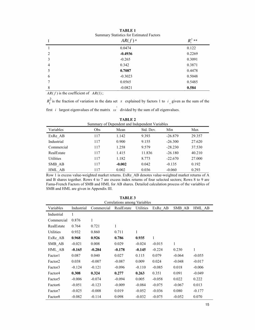
Table 1 reports the cumulative variation in the data explained by Factor 1 to i , given

as the sum of the first i largest eigenvalues of the matrix '

xx divided by the sum of

all eigenvalues. By construction, the factors are mutually orthogonal, and Factor 1

explains the largest fraction of the total variances in the panel data. Factor 2 explains

the largest fraction of the variation in x , controlling for Factor 1, and so on.

INSERT TABLE 1 HERE

The second column shows that a small number of factors account for a large

10

proportion of the variance in the panel dataset, as eight factors account for nearly 60%

of the variation. The first column in the table displays the first-order autoregressive

coefficient for each factor. Most of the factors have a persistence of less than 0.5,

except for Factor 5. This finding coincides with the short-term relationship between

predictor variables and excess returns in this paper. In addition, there is considerable

heterogeneity across the estimated factors, with coefficients of (1)AR regressions

ranging from -0.4936 to 0.7087.

Descriptive Analysis

Table 2 presents the summary of the dependent and predetermined predictors.

INSERT TABLE 2 HERE

Note that real estate stocks are more volatile and generate higher mean excess returns;

this is the opposite for stocks from the industrial sector. One important Macro policy

tool in China is done through the measures for adjusting the real estate market.

Therefore, the real estate stocks comparing to the industrial sector are more volatile

and generate higher mean excess returns.5

Table 3 shows the correlations for the sector indices and explanatory variables. The

correlations among the factors are not presented because they are orthogonal to each

other by construction.

INSERT TABLE 3 HERE

The market premium of Re_Ex AB is considered as a predictor of the sector index

returns, as in the Fama-French model. This market premium is highly correlated with

all the excess index returns, although the coefficient of the real estate sector is

substantially lower. Factor 4 is closely correlated with excess returns and the variable

of _HML AB is more relevant than the variable of _SMB AB . Since the

correlations among independent variables are substantially low, we do not expect a

11

serious multicollinearity problem to be present in the model.

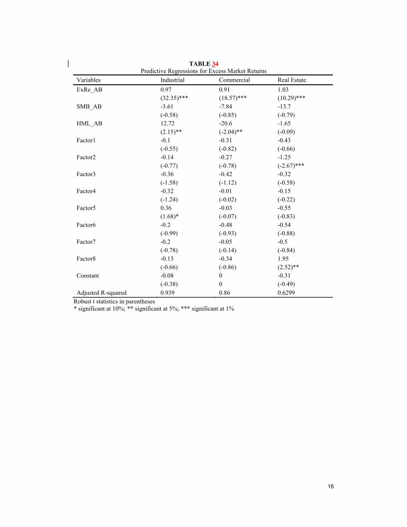
Estimation

The regression coefficients, heteroskedasticity, and serial correlation robust t

-statistics6, and adjusted 2

R statistics are reported in Table 4.

INSERT TABLE 4 HERE.

Factors 4 and 5, the “interest rate related factors”, are found to be important for

predicting monthly excess index returns in utilities and industrial sectors, respectively.

Furthermore, some interesting differences between the four sectors should be noted.

First, in addition to Factor 4, Factor 1, the “output level” factor has good explanatory

power for the excess returns of the utilities index. The negative coefficient is

foreseeable, as Factor 3 is negatively correlated with the data series on industrial

output growth. Therefore, a higher industrial output growth for the present month can

explain higher excess returns in the industrial sector in the next month. The growth in

production in the macro economy is best reflected in industrial stocks returns.

Among all four sectors, HML is important in the industrial and commercial sectors.

Note that the R-squared of the model for the industrial sector is much higher

compared to that of other sectors.

The excess index returns of real estate stocks can be predicted by Factor 2. Note that

the adjusted R-squares only minutely exceed 60% after adding the Fama-French

market premium variable. It is interesting to note that the “property demand factor”

(Factor 7) is not a good predictor, implying that macroeconomic information on real

estate may not be well-integrated into real estate stocks, and returns of property stocks

may not totally reflect the macroeconomic fundamentals of the property sector.

Many of the estimated factors contain information common to that in the predictor

variables, which have long served as conditioning variables. This suggests that the

standard variables do indeed summarize a wide range of information on the economic

12

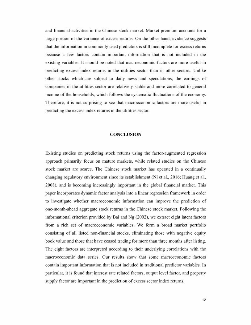
and financial activities in the Chinese stock market. Market premium accounts for a

large portion of the variance of excess returns. On the other hand, evidence suggests

that the information in commonly used predictors is still incomplete for excess returns

because a few factors contain important information that is not included in the

existing variables. It should be noted that macroeconomic factors are more useful in

predicting excess index returns in the utilities sector than in other sectors. Unlike

other stocks which are subject to daily news and speculations, the earnings of

companies in the utilities sector are relatively stable and more correlated to general

income of the households, which follows the systematic fluctuations of the economy.

Therefore, it is not surprising to see that macroeconomic factors are more useful in

predicting the excess index returns in the utilities sector.

CONCLUSION

Existing studies on predicting stock returns using the factor-augmented regression

approach primarily focus on mature markets, while related studies on the Chinese

stock market are scarce. The Chinese stock market has operated in a continually

changing regulatory environment since its establishment (Ni et al., 2016; Huang et al.,

2008), and is becoming increasingly important in the global financial market. This

paper incorporates dynamic factor analysis into a linear regression framework in order

to investigate whether macroeconomic information can improve the prediction of

one-month-ahead aggregate stock returns in the Chinese stock market. Following the

informational criterion provided by Bai and Ng (2002), we extract eight latent factors

from a rich set of macroeconomic variables. We form a broad market portfolio

consisting of all listed non-financial stocks, eliminating those with negative equity

book value and those that have ceased trading for more than three months after listing.

The eight factors are interpreted according to their underlying correlations with the

macroeconomic data series. Our results show that some macroeconomic factors

contain important information that is not included in traditional predictor variables. In

particular, it is found that interest rate related factors, output level factor, and property

supply factor are important in the prediction of excess sector index returns.

13

NOTES

1. Chong et al. (2013) investigate the transmission mechanism of monetary policy in China. It is

found that the repo rate, benchmark lending rate, and a market-based monetary stance have

little impact on the Chinese economy. The non-market-based measures of People's Bank of

China, such as growth rates of total loan and money supply, are effective in adjusting the real

economy and price level.

2. In classic factor analysis model, idiosyncratic disturbances have to be cross-sectionally

independent and temporally independent and identically distributed. These assumptions are

unlikely to be satisfied in our study, as a result, we adopt a dynamic factor structure, in which

the error terms are permitted to be both serially correlated and weakly cross-sectionally

correlated.

3. The number of financial companies is 30, which accounts for only about 1.64% of the total

companies across industries.

4. No more than 150 companies have experienced negative book values starting from 2000, they

are very small percentage of all the listed companies.

5. For the relationship between the real estate market and stock market in China, one is referred

to Zhang and Fung (2006).

6. Newey - West statistic with zero lag.

REFERENCES

Ang, A., Bekaert, G., & Wei, M. (2007). Do macro variables, asset markets, or surveys forecast

inflation better? Journal of Monetary Economics, 54, 1163-1212.

Bai, J. (2010). Equity premium predictions with adaptive macro indexes. Staff Reports no. 475,

Federal Reserve Bank of New York.

Bai, J., & Ng, S. (2002). Determining the number of factors in approximate factor models.

Econometrica, 70, 191-221.

Bai, J., & Ng, S. (2006). Confidence intervals for diffusion index forecasts and inference for

factor-augmented regressions. Econometrica, 74, 1133-1150.

Bernanke, B., Boivin, J., & Eliasz, P. (2005). Measuring the Effects of Monetary Policy: A

Factor-Augmented Vector Autoregressive (FAVAR) Approach. Quarterly Journal of

Economics, 120, 387-422.

Chen, X, & Chiang, T. C. (2016). Stock returns and economic forces—An empirical investigation

of Chinese markets. Global Finance Journal, 30, 45–65.

Chen, N. (1991). Financial investment opportunities and the macroeconomy. Journal of Finance,

46, 529-554.

Chen, N., Roll, R., Ross, S. (1986). Economic forces and the stock market. Journal of Business, 59,

383-403.

Chong, T. T. L., Leung, P. H., & He, Q. (2013). Factor-augmented VAR analysis of the monetary

policy in China. China Economic Review, 25, 88-104.

Connor, G., & Korajczyk, R. (1986). Performance measurement with the arbitrage pricing theory:

14

A new framework for analysis. Journal of Financial Economics, 15, 373-394.

Fama, E., & French, K. (1992). The cross-section of expected stock returns. The Journal of

Finance, 47, 427-465.

Fama, E., & French, K. (1988). Dividend yields and expected stock returns. Journal of Financial

Economics, 22, 3-25.

Goh, J.C., Jiang, F., Tu, J., & Wang, Y. (2013). Can US economic variables predict the Chinese

stock market? Pacific-Basin Finance Journal, 22, 69–87.

Hamao, Y. (1988). An empirical examination of the Arbitrage Pricing Theory: Using Japanese

data. Japan and the World Economy, 1, 45-61.

Huang, F., Su, J., & Chong, T. T. L. (2008). Testing for Structural Change in the Nontradable

Share Reform of the Chinese Stock Market. The Chinese Economy, 41(2), 24-33.

Jensen, G., Mercer, J., & Johnson, R. (1996). Business conditions, monetary policy, and expected

security returns. Journal of Financial Economics, 40, 213-237.

Lamont, O. (2000). Investment plans and stock returns. Journal of Finance, 55, 2719-2745.

Lettau, M., & Ludvigson, S. (2001). Consumption, aggregate wealth, and expected stock returns.

Journal of Finance, 56, 815-849.

Liang, P., & Willett, D. (2015). Chinese stocks during 2000–2013: Bubbles and busts or

fundamentals? The Chinese Economy, 48(3), 26-39.

Ludvigson, S., & Ng, S. (2007). The empirical risk-return relation: A factor analysis approach.

Journal of Financial Economics, 83, 171-222.

Ludvigson, S., Ng, S. (2009). Macro factors in bond risk premia. Review of Financial Studies,

22(12), 5027-5067.

Ni, J., Wohar, M. E., & Wang B. (2016). Structural breaks in volatility: The case of Chinese stock

returns. The Chinese Economy, 49(2), 81-93.

Shanken, J., Weinstein, M. (1990). Macroeconomic variables and asset pricing: Further results.

Manuscript University of Southern California.

Stock, J., & Watson, M. (2002a). Forecasting using principal components from a large number of

predictors. Journal of the American Statistical Association, 97, 1167-1179.

Stock, J., & Watson, M. (2002b). Macroeconomic forecasting using diffusion indexes. Journal of

Business and Economic Statistics, 20(2), 147-162.

Wang, F., & Xu, Y. (2004). What determines Chinese stock returns? Financial Analysts Journal,

60, 65-77.

Welch, I., Goyal, A., 2008. A comprehensive look at the empirical performance of equity

premium prediction. Review of Financial Studies, 21(4), 1455-1508.

Zhang, G., & Fung, H. G. (2006). On the imbalance between the real estate market and the stock

markets in China. The Chinese Economy, 39(2), 26-39.

15

TABLE 1 Summary Statistics for Estimated Factors

I ( )AR f * 2

iR **

1 0.0474 0.122

2 -0.4936 0.2269

3 -0.265 0.3091

4 0.342 0.3871

5 0.7087 0.4478

6 -0.3023 0.5048

7 0.0565 0.5485

8 -0.0821 0.584

( )AR f is the coefficient of (1)AR ;

2i

R is the fraction of variation in the data set x explained by factors 1 to i , given as the sum of the

first i largest eigenvalues of the matrix '

xx divided by the sum of all eigenvalues.

TABLE 2

Summary of Dependent and Independent Variables

Variables Obs Mean Std. Dev. Min Max

ExRe_AB 117 1.142 9.393 -26.879 29.357

Industrial 117 0.900 9.155 -26.300 27.620

Commercial 117 1.258 9.579 -28.230 37.530

RealEstate 117 1.415 11.836 -26.180 40.210

Utilities 117 1.182 8.773 -22.670 27.000

SMB_AB 117 -0.002 0.042 -0.135 0.192

HML_AB 117 0.002 0.036 -0.060 0.293

Row 1 is excess value-weighted market returns. ExRe_AB denotes value-weighted market returns of A

and B shares together. Rows 4 to 7 are excess index returns of four selected sectors; Rows 8 to 9 are

Fama-French Factors of SMB and HML for AB shares. Detailed calculation process of the variables of

SMB and HML are given in Appendix III.

TABLE 3

Correlations among Variables

Variables Industrial Commercial RealEstate Utilities ExRe_AB SMB_AB HML_AB

Industrial 1

Commercial 0.876 1

RealEstate 0.764 0.721 1

Utilities 0.932 0.860 0.711 1

ExRe_AB 0.968 0.926 0.786 0.935 1

SMB_AB -0.021 0.008 0.029 -0.024 -0.015 1

HML_AB -0.165 -0.284 -0.178 -0.145 -0.224 0.230 1

Factor1 0.087 0.040 0.027 0.115 0.079 -0.064 -0.055

Factor2 0.038 -0.007 -0.087 0.009 0.024 -0.048 -0.017

Factor3 -0.124 -0.121 -0.096 -0.110 -0.085 0.018 -0.006

Factor4 0.308 0.324 0.277 0.263 0.351 0.091 -0.049

Factor5 -0.006 -0.074 -0.094 0.005 -0.058 0.022 0.222

Factor6 -0.051 -0.123 -0.009 -0.084 -0.075 -0.067 0.013

Factor7 -0.025 -0.008 0.019 -0.052 -0.036 0.080 -0.177

Factor8 -0.082 -0.114 0.098 -0.032 -0.075 -0.052 0.070

16

TABLE 34

Predictive Regressions for Excess Market Returns

Variables Industrial Commercial Real Estate

ExRe_AB 0.97 0.91 1.03

(32.35)*** (18.57)*** (10.29)***

SMB_AB -3.61 -7.84 -13.7

(-0.58) (-0.85) (-0.79)

HML_AB 12.72 -20.6 -1.65

(2.15)** (-2.04)** (-0.09)

Factor1 -0.1 -0.31 -0.43

(-0.55) (-0.82) (-0.66)

Factor2 -0.14 -0.27 -1.25

(-0.77) (-0.78) (-2.67)***

Factor3 -0.36 -0.42 -0.32

(-1.58) (-1.12) (-0.58)

Factor4 -0.32 -0.01 -0.15

(-1.24) (-0.02) (-0.22)

Factor5 0.36 -0.03 -0.55

(1.68)* (-0.07) (-0.83)

Factor6 -0.2 -0.48 -0.54

(-0.99) (-0.93) (-0.88)

Factor7 -0.2 -0.05 -0.5

(-0.78) (-0.14) (-0.84)

Factor8 -0.13 -0.34 1.95

(-0.66) (-0.86) (2.52)**

Constant -0.08 0 -0.31

(-0.38) 0 (-0.49)

Adjusted R-squared 0.939 0.86 0.6299

Robust t statistics in parentheses * significant at 10%; ** significant at 5%; *** significant at 1%

17

FIGURE 1 Marginal R-squares on macroeconomic series of factor 1

-0.1

0

0.1

0.2

0.3

0.4

0.5

0.6

0.7

1 6 11 16 21 26 31 36 41 46 51 56 61 66 71 76 81 86 91 96 101 106 111 116 121

R-s

qu

are

s

Output Property Enterp. Gov. Consum. Price IM&EX Liquidity IR&ER

18


-0.1

0

0.1

0.2

0.3

0.4

0.5

0.6

0.7

0.8

1 6 11 16 21 26 31 36 41 46 51 56 61 66 71 76 81 86 91 96 101 106 111 116 121

R-s

qu

are

s


19


-0.1

0

0.1

0.2

0.3

0.4

0.5

0.6

0.7

1 6 11 16 21 26 31 36 41 46 51 56 61 66 71 76 81 86 91 96 101 106 111 116 121

R-s

qu

are

s


20


-0.05

0

0.05

0.1

0.15

0.2

0.25

0.3

0.35

0.4

1 6 11 16 21 26 31 36 41 46 51 56 61 66 71 76 81 86 91 96 101 106 111 116 121

R-s

qu

are

s


21


-0.1

0

0.1

0.2

0.3

0.4

0.5

1 6 11 16 21 26 31 36 41 46 51 56 61 66 71 76 81 86 91 96 101 106 111 116 121

R-s

qu

are

s


22


-0.1

0

0.1

0.2

0.3

0.4

0.5

0.6

1 6 11 16 21 26 31 36 41 46 51 56 61 66 71 76 81 86 91 96 101 106 111 116 121

R-s

qu

are

s


23


-0.1

0

0.1

0.2

0.3

0.4

0.5

0.6

1 6 11 16 21 26 31 36 41 46 51 56 61 66 71 76 81 86 91 96 101 106 111 116 121

R-s

qu

are

s


24


-0.05

0

0.05

0.1

0.15

0.2

0.25

1 6 11 16 21 26 31 36 41 46 51 56 61 66 71 76 81 86 91 96 101 106 111 116 121

R-s

qu

are

s


25

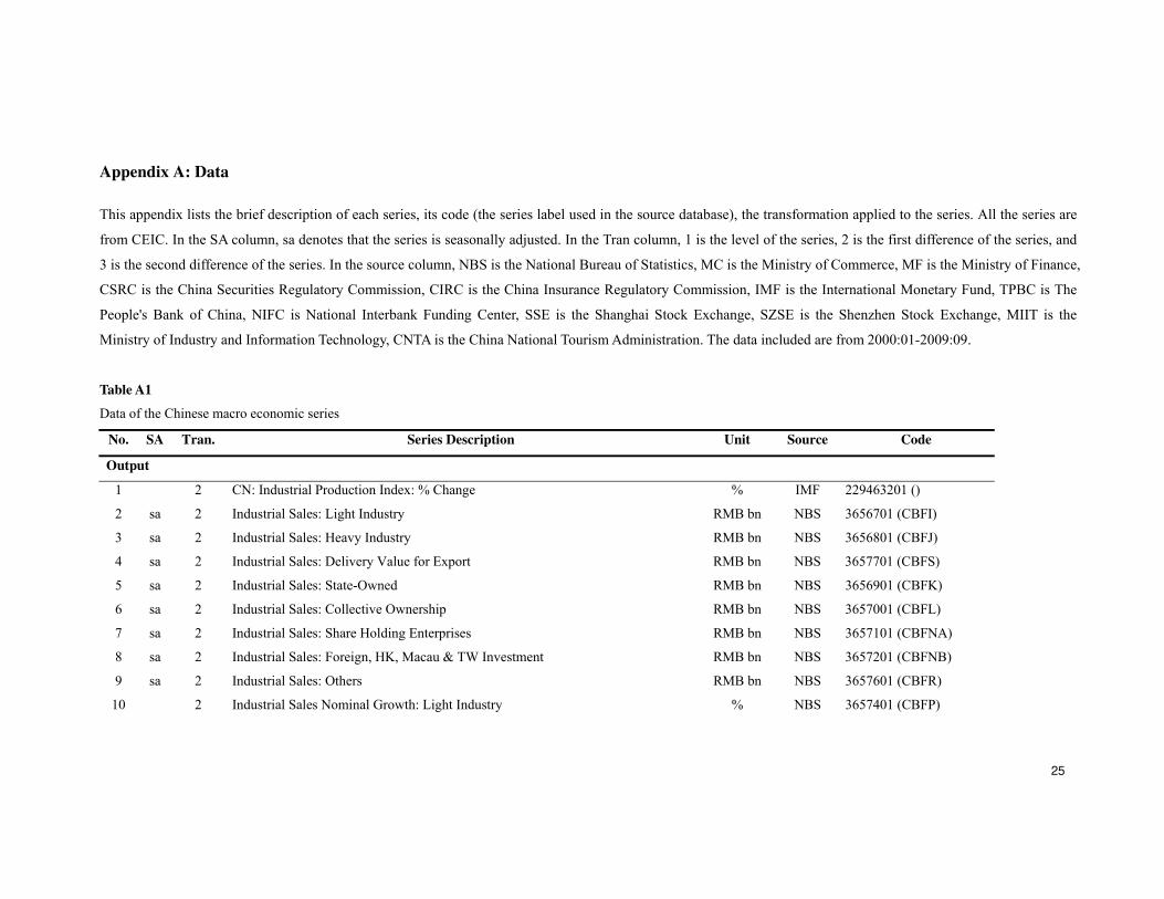
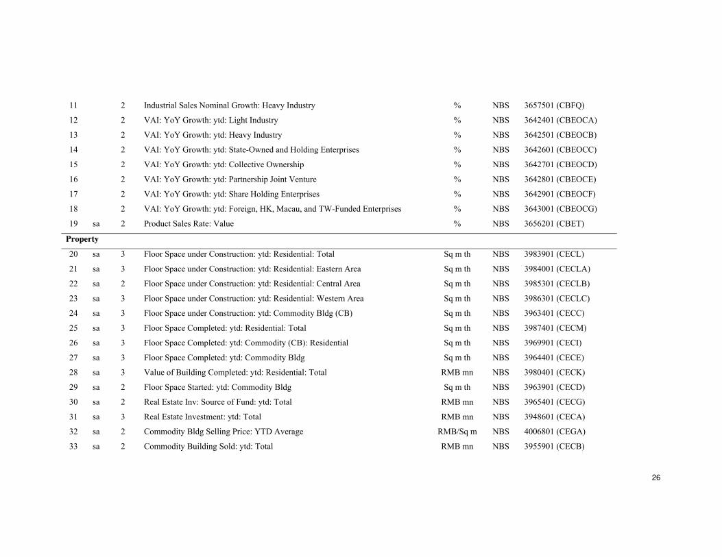
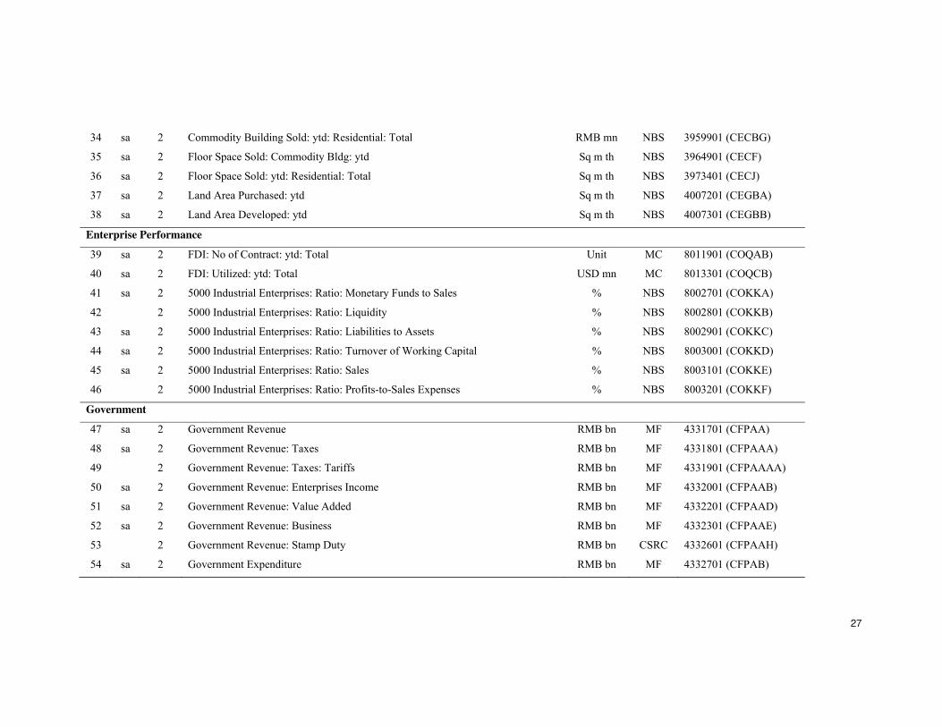
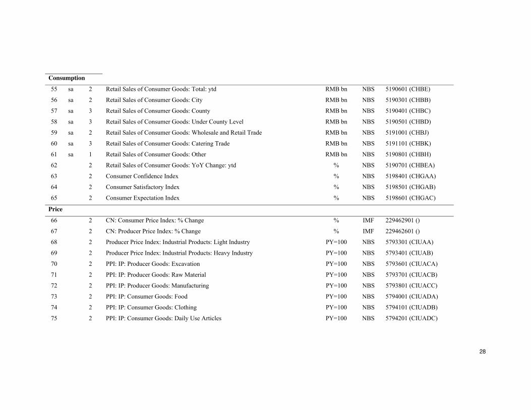
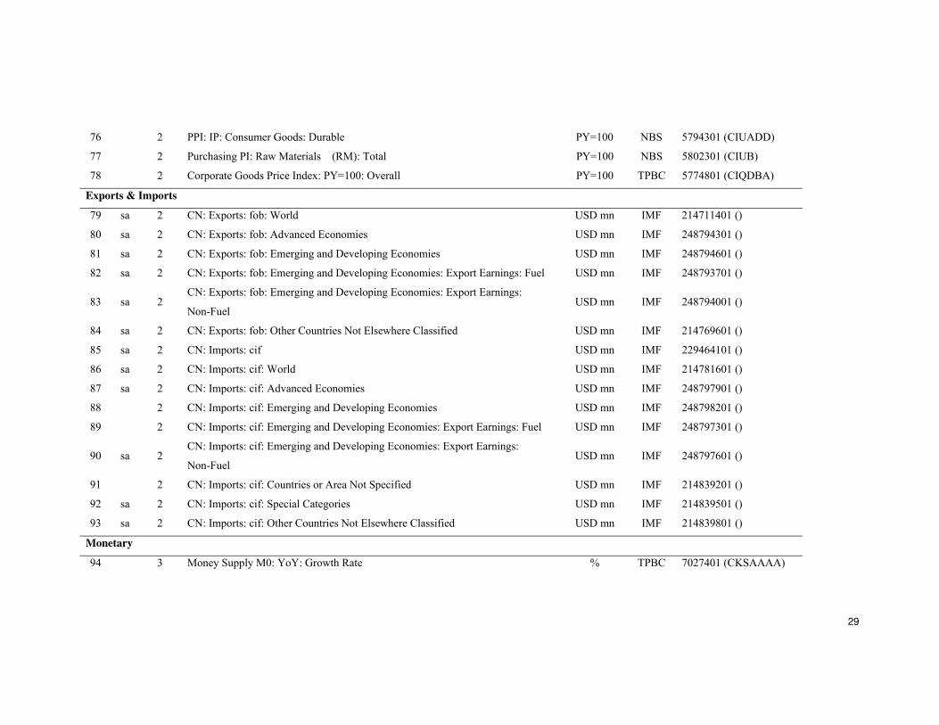
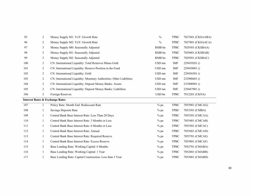
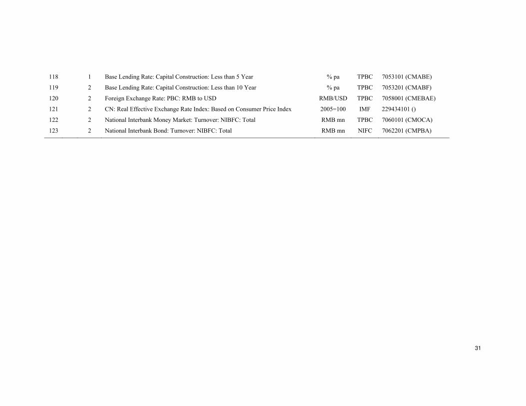
Appendix A: Data

This appendix lists the brief description of each series, its code (the series label used in the source database), the transformation applied to the series. All the series are

from CEIC. In the SA column, sa denotes that the series is seasonally adjusted. In the Tran column, 1 is the level of the series, 2 is the first difference of the series, and

3 is the second difference of the series. In the source column, NBS is the National Bureau of Statistics, MC is the Ministry of Commerce, MF is the Ministry of Finance,

CSRC is the China Securities Regulatory Commission, CIRC is the China Insurance Regulatory Commission, IMF is the International Monetary Fund, TPBC is The

People's Bank of China, NIFC is National Interbank Funding Center, SSE is the Shanghai Stock Exchange, SZSE is the Shenzhen Stock Exchange, MIIT is the

Ministry of Industry and Information Technology, CNTA is the China National Tourism Administration. The data included are from 2000:01-2009:09.

Table A1

Data of the Chinese macro economic series

No. SA Tran. Series Description Unit Source Code

Output

1 2 CN: Industrial Production Index: % Change % IMF 229463201 ()

2 sa 2 Industrial Sales: Light Industry RMB bn NBS 3656701 (CBFI)

3 sa 2 Industrial Sales: Heavy Industry RMB bn NBS 3656801 (CBFJ)

4 sa 2 Industrial Sales: Delivery Value for Export RMB bn NBS 3657701 (CBFS)

5 sa 2 Industrial Sales: State-Owned RMB bn NBS 3656901 (CBFK)

6 sa 2 Industrial Sales: Collective Ownership RMB bn NBS 3657001 (CBFL)

7 sa 2 Industrial Sales: Share Holding Enterprises RMB bn NBS 3657101 (CBFNA)

8 sa 2 Industrial Sales: Foreign, HK, Macau & TW Investment RMB bn NBS 3657201 (CBFNB)

9 sa 2 Industrial Sales: Others RMB bn NBS 3657601 (CBFR)

10 2 Industrial Sales Nominal Growth: Light Industry % NBS 3657401 (CBFP)

26

11 2 Industrial Sales Nominal Growth: Heavy Industry % NBS 3657501 (CBFQ)

12 2 VAI: YoY Growth: ytd: Light Industry % NBS 3642401 (CBEOCA)

13 2 VAI: YoY Growth: ytd: Heavy Industry % NBS 3642501 (CBEOCB)

14 2 VAI: YoY Growth: ytd: State-Owned and Holding Enterprises % NBS 3642601 (CBEOCC)

15 2 VAI: YoY Growth: ytd: Collective Ownership % NBS 3642701 (CBEOCD)

16 2 VAI: YoY Growth: ytd: Partnership Joint Venture % NBS 3642801 (CBEOCE)

17 2 VAI: YoY Growth: ytd: Share Holding Enterprises % NBS 3642901 (CBEOCF)

18 2 VAI: YoY Growth: ytd: Foreign, HK, Macau, and TW-Funded Enterprises % NBS 3643001 (CBEOCG)

19 sa 2 Product Sales Rate: Value % NBS 3656201 (CBET)

Property

20 sa 3 Floor Space under Construction: ytd: Residential: Total Sq m th NBS 3983901 (CECL)

21 sa 3 Floor Space under Construction: ytd: Residential: Eastern Area Sq m th NBS 3984001 (CECLA)

22 sa 2 Floor Space under Construction: ytd: Residential: Central Area Sq m th NBS 3985301 (CECLB)

23 sa 3 Floor Space under Construction: ytd: Residential: Western Area Sq m th NBS 3986301 (CECLC)

24 sa 3 Floor Space under Construction: ytd: Commodity Bldg (CB) Sq m th NBS 3963401 (CECC)

25 sa 3 Floor Space Completed: ytd: Residential: Total Sq m th NBS 3987401 (CECM)

26 sa 3 Floor Space Completed: ytd: Commodity (CB): Residential Sq m th NBS 3969901 (CECI)

27 sa 3 Floor Space Completed: ytd: Commodity Bldg Sq m th NBS 3964401 (CECE)

28 sa 3 Value of Building Completed: ytd: Residential: Total RMB mn NBS 3980401 (CECK)

29 sa 2 Floor Space Started: ytd: Commodity Bldg Sq m th NBS 3963901 (CECD)

30 sa 2 Real Estate Inv: Source of Fund: ytd: Total RMB mn NBS 3965401 (CECG)

31 sa 3 Real Estate Investment: ytd: Total RMB mn NBS 3948601 (CECA)

32 sa 2 Commodity Bldg Selling Price: YTD Average RMB/Sq m NBS 4006801 (CEGA)

33 sa 2 Commodity Building Sold: ytd: Total RMB mn NBS 3955901 (CECB)

27

34 sa 2 Commodity Building Sold: ytd: Residential: Total RMB mn NBS 3959901 (CECBG)

35 sa 2 Floor Space Sold: Commodity Bldg: ytd Sq m th NBS 3964901 (CECF)

36 sa 2 Floor Space Sold: ytd: Residential: Total Sq m th NBS 3973401 (CECJ)

37 sa 2 Land Area Purchased: ytd Sq m th NBS 4007201 (CEGBA)

38 sa 2 Land Area Developed: ytd Sq m th NBS 4007301 (CEGBB)

Enterprise Performance

39 sa 2 FDI: No of Contract: ytd: Total Unit MC 8011901 (COQAB)

40 sa 2 FDI: Utilized: ytd: Total USD mn MC 8013301 (COQCB)

41 sa 2 5000 Industrial Enterprises: Ratio: Monetary Funds to Sales % NBS 8002701 (COKKA)

42 2 5000 Industrial Enterprises: Ratio: Liquidity % NBS 8002801 (COKKB)

43 sa 2 5000 Industrial Enterprises: Ratio: Liabilities to Assets % NBS 8002901 (COKKC)

44 sa 2 5000 Industrial Enterprises: Ratio: Turnover of Working Capital % NBS 8003001 (COKKD)

45 sa 2 5000 Industrial Enterprises: Ratio: Sales % NBS 8003101 (COKKE)

46 2 5000 Industrial Enterprises: Ratio: Profits-to-Sales Expenses % NBS 8003201 (COKKF)

Government

47 sa 2 Government Revenue RMB bn MF 4331701 (CFPAA)

48 sa 2 Government Revenue: Taxes RMB bn MF 4331801 (CFPAAA)

49 2 Government Revenue: Taxes: Tariffs RMB bn MF 4331901 (CFPAAAA)

50 sa 2 Government Revenue: Enterprises Income RMB bn MF 4332001 (CFPAAB)

51 sa 2 Government Revenue: Value Added RMB bn MF 4332201 (CFPAAD)

52 sa 2 Government Revenue: Business RMB bn MF 4332301 (CFPAAE)

53 2 Government Revenue: Stamp Duty RMB bn CSRC 4332601 (CFPAAH)

54 sa 2 Government Expenditure RMB bn MF 4332701 (CFPAB)

28

Consumption

55 sa 2 Retail Sales of Consumer Goods: Total: ytd RMB bn NBS 5190601 (CHBE)

56 sa 2 Retail Sales of Consumer Goods: City RMB bn NBS 5190301 (CHBB)

57 sa 3 Retail Sales of Consumer Goods: County RMB bn NBS 5190401 (CHBC)

58 sa 3 Retail Sales of Consumer Goods: Under County Level RMB bn NBS 5190501 (CHBD)

59 sa 2 Retail Sales of Consumer Goods: Wholesale and Retail Trade RMB bn NBS 5191001 (CHBJ)

60 sa 3 Retail Sales of Consumer Goods: Catering Trade RMB bn NBS 5191101 (CHBK)

61 sa 1 Retail Sales of Consumer Goods: Other RMB bn NBS 5190801 (CHBH)

62 2 Retail Sales of Consumer Goods: YoY Change: ytd % NBS 5190701 (CHBEA)

63 2 Consumer Confidence Index % NBS 5198401 (CHGAA)

64 2 Consumer Satisfactory Index % NBS 5198501 (CHGAB)

65 2 Consumer Expectation Index % NBS 5198601 (CHGAC)

Price

66 2 CN: Consumer Price Index: % Change % IMF 229462901 ()

67 2 CN: Producer Price Index: % Change % IMF 229462601 ()

68 2 Producer Price Index: Industrial Products: Light Industry PY=100 NBS 5793301 (CIUAA)

69 2 Producer Price Index: Industrial Products: Heavy Industry PY=100 NBS 5793401 (CIUAB)

70 2 PPI: IP: Producer Goods: Excavation PY=100 NBS 5793601 (CIUACA)

71 2 PPI: IP: Producer Goods: Raw Material PY=100 NBS 5793701 (CIUACB)

72 2 PPI: IP: Producer Goods: Manufacturing PY=100 NBS 5793801 (CIUACC)

73 2 PPI: IP: Consumer Goods: Food PY=100 NBS 5794001 (CIUADA)

74 2 PPI: IP: Consumer Goods: Clothing PY=100 NBS 5794101 (CIUADB)

75 2 PPI: IP: Consumer Goods: Daily Use Articles PY=100 NBS 5794201 (CIUADC)

29

76 2 PPI: IP: Consumer Goods: Durable PY=100 NBS 5794301 (CIUADD)

77 2 Purchasing PI: Raw Materials (RM): Total PY=100 NBS 5802301 (CIUB)

78 2 Corporate Goods Price Index: PY=100: Overall PY=100 TPBC 5774801 (CIQDBA)

Exports & Imports

79 sa 2 CN: Exports: fob: World USD mn IMF 214711401 ()

80 sa 2 CN: Exports: fob: Advanced Economies USD mn IMF 248794301 ()

81 sa 2 CN: Exports: fob: Emerging and Developing Economies USD mn IMF 248794601 ()

82 sa 2 CN: Exports: fob: Emerging and Developing Economies: Export Earnings: Fuel USD mn IMF 248793701 ()

83 sa 2 CN: Exports: fob: Emerging and Developing Economies: Export Earnings:

Non-Fuel USD mn IMF 248794001 ()

84 sa 2 CN: Exports: fob: Other Countries Not Elsewhere Classified USD mn IMF 214769601 ()

85 sa 2 CN: Imports: cif USD mn IMF 229464101 ()

86 sa 2 CN: Imports: cif: World USD mn IMF 214781601 ()

87 sa 2 CN: Imports: cif: Advanced Economies USD mn IMF 248797901 ()

88 2 CN: Imports: cif: Emerging and Developing Economies USD mn IMF 248798201 ()

89 2 CN: Imports: cif: Emerging and Developing Economies: Export Earnings: Fuel USD mn IMF 248797301 ()

90 sa 2 CN: Imports: cif: Emerging and Developing Economies: Export Earnings:

Non-Fuel USD mn IMF 248797601 ()

91 2 CN: Imports: cif: Countries or Area Not Specified USD mn IMF 214839201 ()

92 sa 2 CN: Imports: cif: Special Categories USD mn IMF 214839501 ()

93 sa 2 CN: Imports: cif: Other Countries Not Elsewhere Classified USD mn IMF 214839801 ()

Monetary

94 3 Money Supply M0: YoY: Growth Rate % TPBC 7027401 (CKSAAAA)

30

95 2 Money Supply M1: YoY: Growth Rate % TPBC 7027601 (CKSAABA)

96 2 Money Supply M2: YoY: Growth Rate % TPBC 7027801 (CKSAACA)

97 3 Money Supply M0: Seasonally Adjusted RMB bn TPBC 7029301 (CKSBAA)

98 3 Money Supply M1: Seasonally Adjusted RMB bn TPBC 7029401 (CKSBAB)

99 3 Money Supply M2: Seasonally Adjusted RMB bn TPBC 7029501 (CKSBAC)

100 2 CN: International Liquidity: Total Reserves Minus Gold USD mn IMF 229439201 ()

101 2 CN: International Liquidity: Reserve Position in the Fund USD mn IMF 229438001 ()

102 2 CN: International Liquidity: Gold USD mn IMF 229436501 ()

103 2 CN: International Liquidity: Monetary Authorities: Other Liabilities USD mn IMF 232908601 ()

104 2 CN: International Liquidity: Deposit Money Banks: Assets USD mn IMF 232908901 ()

105 2 CN: International Liquidity: Deposit Money Banks: Liabilities USD mn IMF 229447901 ()

106 3 Foreign Reserves USD bn TPBC 7012201 (CKNA)

Interest Rates & Exchange Rates

107 1 Policy Rate: Month End: Rediscount Rate % pa TPBC 7055901 (CMCAG)

108 1 Savings Deposits Rate % pa TPBC 7053301 (CMBA)

109 1 Central Bank Base Interest Rate: Less Than 20 Days % pa TPBC 7055301 (CMCAA)

110 1 Central Bank Base Interest Rate: 3 Months or Less % pa TPBC 7055401 (CMCAB)

111 1 Central Bank Base Interest Rate: 6 Months or Less % pa TPBC 7055501 (CMCAC)

112 1 Central Bank Base Interest Rate: Annual % pa TPBC 7055601 (CMCAD)

113 1 Central Bank Base Interest Rate: Required Reserve % pa TPBC 7055701 (CMCAE)

114 1 Central Bank Base Interest Rate: Excess Reserve % pa TPBC 7055801 (CMCAF)

115 2 Base Lending Rate: Working Capital: 6 Months % pa TPBC 7052701 (CMABA)

116 1 Base Lending Rate: Working Capital: 1 Year % pa TPBC 7052801 (CMABB)

117 1 Base Lending Rate: Capital Construction: Less than 3 Year % pa TPBC 7053001 (CMABD)

31

118 1 Base Lending Rate: Capital Construction: Less than 5 Year % pa TPBC 7053101 (CMABE)

119 2 Base Lending Rate: Capital Construction: Less than 10 Year % pa TPBC 7053201 (CMABF)

120 2 Foreign Exchange Rate: PBC: RMB to USD RMB/USD TPBC 7058001 (CMEBAE)

121 2 CN: Real Effective Exchange Rate Index: Based on Consumer Price Index 2005=100 IMF 229434101 ()

122 2 National Interbank Money Market: Turnover: NIBFC: Total RMB mn TPBC 7060101 (CMOCA)

123 2 National Interbank Bond: Turnover: NIBFC: Total RMB mn NIFC 7062201 (CMPBA)

Documents

A New Approach to Modelling Sector Stock Returns in China · A New Approach to Modelling Sector Stock Returns in China Chong, Terence Tai Leung and Li, Nasha and Zou, Lin The Chinese