Embed Size (px)
Citation preview

A NEW APPROACH TO DATINGTHE REFERENCE CYCLE
Máximo Camacho, María Dolores Gadeaand Ana Gómez Loscos
Documentos de Trabajo N.º 1914
2019

A NEW APPROACH TO DATING THE REFERENCE CYCLE

A NEW APPROACH TO DATING THE REFERENCE CYCLE (*)
Máximo Camacho (**)
UNIVERSITY OF MURCIA
María Dolores Gadea (***)
UNIVERSITY OF ZARAGOZA
Ana Gómez Loscos (****)
BANCO DE ESPAÑA
Documentos de Trabajo. N.º 1914
2019
(*) M. Camacho and M. D. Gadea are grateful for the support of grants ECO2016-76178-P, 19884/GERM/15, and ECO2017-83255-C3-1-P and ECO2017-83255-C3-3-P (MICINU, AEI/ERDF, EU), respectively. All remaining errors are our responsibility. Data and codes that replicate our results are available from the authors’ websites. The views in this paper are those of the authors and do not represent the views of the Banco de España or the Eurosystem.(**) Department of Quantitative Analysis, University of Murcia. Campus de Espinardo, 30100 Murcia (Spain). Tel.: +34 868887982, fax: +34 868887905 and e-mail: [email protected].(***) Department of Applied Economics, University of Zaragoza. Gran Vía, 4, 50005 Zaragoza (Spain). Tel.: +34 976761842, fax: +34 976761840 and e-mail: [email protected].(****) Banco de España, Alcalá, 48, 28014 Madrid (Spain). Tel.: +34 913385817, fax: +34 915310059 and e-mail: [email protected].

The Working Paper Series seeks to disseminate original research in economics and fi nance. All papers have been anonymously refereed. By publishing these papers, the Banco de España aims to contribute to economic analysis and, in particular, to knowledge of the Spanish economy and its international environment.
The opinions and analyses in the Working Paper Series are the responsibility of the authors and, therefore, do not necessarily coincide with those of the Banco de España or the Eurosystem.
The Banco de España disseminates its main reports and most of its publications via the Internet at the following website: http://www.bde.es.
Reproduction for educational and non-commercial purposes is permitted provided that the source is acknowledged.
© BANCO DE ESPAÑA, Madrid, 2019
ISSN: 1579-8666 (on line)

Abstract
This paper proposes a new approach to the analysis of the reference cycle turning points,
defi ned on the basis of the specifi c turning points of a broad set of coincident economic
indicators. Each individual pair of specifi c peaks and troughs from these indicators is
viewed as a realization of a mixture of an unspecifi ed number of separate bivariate Gaussian
distributions whose different means are the reference turning points. These dates break the
sample into separate reference cycle phases, whose shifts are modeled by a hidden Markov
chain. The transition probability matrix is constrained so that the specifi cation is equivalent
to a multiple changepoint model. Bayesian estimation of fi nite Markov mixture modeling
techniques is suggested to estimate the model. Several Monte Carlo experiments are used
to show the accuracy of the model to date reference cycles that suffer from short phases,
uncertain turning points, small samples and asymmetric cycles. In the empirical section, we
show the high performance of our approach to identifying the US reference cycle, with little
difference from the timing of the turning point dates established by the NBER. In a pseudo
real-time analysis, we also show the good performance of this methodology in terms of
accuracy and speed of detection of turning point dates.
Keywords: business cycles, turning points, fi nite mixture models.
JEL classifi cation: E32, C22, E27.

Resumen
Este trabajo propone un nuevo procedimiento para estimar el fechado de los cambios
de fase (picos y valles) en un ciclo económico de referencia, a partir del fechado de los
cambios de fase en los ciclos económicos específi cos de un conjunto amplio de indicadores
económicos coincidentes. Cada pareja de picos y de valles específi cos, obtenida a partir
de esos indicadores, se considera una realización de una mixtura de un número
no especifi cado de distintas distribuciones gaussianas bivariantes, cuyas esperanzas
son los picos y los valles del ciclo de referencia. Las transiciones se modelizan a partir de una
cadena de Markov equivalente a un modelo de múltiples cambios estructurales.
Los parámetros se estiman con técnicas bayesianas. Con simulaciones de Monte Carlo,
se muestra la capacidad del modelo para fechar los cambios de fase de los ciclos económicos
de referencia generados, que incluyen características cíclicas muy diversas. Además, se
ilustra el funcionamiento empírico del modelo para determinar el fechado histórico del ciclo
de referencia de Estados Unidos a partir de un conjunto de indicadores económicos,
y se obtienen picos y valles muy similares a los del NBER. Por último, se realiza un
análisis en pseudo tiempo real, donde se muestran la precisión y la rapidez en la detección
de los puntos de cambio de fase cíclica.
Palabras clave: ciclos económicos, fechado de los puntos de cambio de fase cíclica,
modelos de Markov con mixturas fi nitas de distribuciones.
Códigos JEL: E32, C22, E27.

BANCO DE ESPAÑA 7 DOCUMENTO DE TRABAJO N.º 1914
1On the contrary, the average-then-date approach focuses on one (or a few) highly aggregated time series to datethe reference cycle.
2They define the different episodes as the NBER turning point dates ±12 months.
1 Introduction
Since the early work of Burns and Mitchell (1946), a classical problem in business cycle analysis has
been to make inferences about the reference cycle dates. These authors postulate that reference
cycle turning point dates can be identified by searching for clusters in specific cycle turning point
dates from a set of disaggregated coincident economic indicators, which typically cluster around
periods of recoveries and declines. In practice, although the distribution of the turning points of the
disaggregated series are routinely achieved by employing dating algorithms such as the monthly Bry
and Boschan (1971) and the quarterly Harding and Pagan (2002) procedures, the main challenge
of this date-then-average literature is to determine the aggregated reference cycle based on these
specific dates.1
From a set of series that are believed to be roughly coincident, Burns and Mitchell (1946) seek
to identify clusters of specific turning points by visual inspection. The authors mark off the zone
within which a succession of specific turning points cluster together with a central tendency and
proceed to refine the approximate dates based on expert judgment by a sequential process of trial
and error. Therefore, the procedure depends on judgments that inevitably condition the reference
dates and make it difficult to replicate and update.
Harding and Pagan (2006) is the first modern contribution to the approach of clustering specific
turning points to obtain reference dates. These authors consider individual turning points as sample
realizations of a (relatively small) number of economic indicators and propose a nonparametric
algorithm to codify the procedures used for extracting the economy-wide turning points. The
algorithm, which is updated in Harding and Pagan (2016), consists of a set of specific rules and
censoring procedures that find the dates that minimize a measure of the average distance between
these dates and the turning points in individual series. Chauvet and Piger (2008) examine the
ability of this algorithm to identify the NBER-referenced business cycle turning point dates in real
time.
Stock and Watson (2010) provide an interesting contribution by computing the reference cycles
as the means of individual series of turning points. Assuming a segmentation of the time span into
business cycle episodes, the data have a standard panel data structure. Then, the parameters can
be estimated by ordinary least squares in a specification with fixed effects, an unbalanced panel
and missing observations. Although the method contributes by producing standard errors for the
estimated reference cycle turning point dates, it takes the sequence of business cycles as given,
which considerably limits its empirical implementation.
Stock and Watson (2014) innovate in this literature by considering turning points as population
concepts. In their approach, turning points are local measures of the central tendency of the
population distribution of the set of disaggregated coincident economic indicators. In particular,
they focus on the mode as the estimator of the tendency of the kernel density of the sample of
individual turning point dates, conditional on the occurrence of a single phase shift in a given
episode covering a known time interval.2 One significant advantage of this framework is that
it provides the asymptotic distributions of the estimator, which allows them to make statistical
inference about the estimated reference cycle. However, they acknowledge that a natural extension
BANCO DE ESPAÑA 8 DOCUMENTO DE TRABAJO N.º 1914
of their method would be to examine estimators that simultaneously determine whether there is a
turning point and, if so, the date of the turning point.
This paper addresses the issue of determining the reference cycle by proposing an alternative
approach that overcomes the drawbacks of the existing methods and that can be implemented
making very minimal distributional assumptions. Our approach assumes that each individual pair
of peak and trough dates is a realization of a mixture of an unspecified number of separate bivariate
Gaussian distributions. The reference cycle dates are viewed as the means of these distributions,
around which the specific dates are clustered, breaking the time span of interest into segments cor-
responding to the periods occupied by the business cycles. The phase shifts across these cycles are
modeled by a discrete-time, discrete-state Markov process with the non-ergodic transition proba-
bility matrix constrained so that the model is equivalent to a multiple change-point model following
the lines suggested by Chib (1998). In this context, we use finite mixture models techniques to
determine the number of turning points of the reference cycle, to estimate the parameters for the
separate distributions, and to make statistical inference about the estimated reference cycle.
Therefore, our research contributes to the literature in several important ways. First, the
aggregate turning points are viewed as population concepts as in Stock and Watson (2010, 2014),
in our case, the distinct means of the separate Gaussian distributions. However, in our approach, the
estimates are not conditional on the known occurrence of a phase shift because both the number
and the dates of the turning points are estimated through the data in a single step. Second,
the method is also able to make statistical inference about the reference cycle turning points.
Consequently, one can evaluate the uncertainty in the determination of the turning point dates
by, for example, computing their confidence or credible intervals. Third, we extend the univariate
multiple change-point model of Chib (1998) to a multivariate framework.
We evaluate the ability of the mixture multiple-point change model to make statistical inference
about a reference cycle by means of several Monte Carlo experiments that try to capture some
basic stylized facts that characterize business cycle fluctuations. Among them, we include double
dip recessions, uncertain turning points, short samples of specific turning points and asymmetric
cycles, which appear when the disaggregated economic indicators are not roughly coincident. With
these simulations, we show that the model exhibits a remarkably high performance in determining
the number of distinct clusters, and that business cycle inferences and parameter estimates are
computed very accurately, even in the presence of these business cycle features.
Finally, we perform an empirical application that illustrates how the method developed in
this paper can be used by practitioners seeking to construct NBER-like reference cycles. The
disaggregated coincident economic indicators used to determine the reference cycle is the set of ten
monthly coincident indicators used by the Business Cycle Committee when determining the trough
of the Great Recession in the US. The estimated model, applied to the Bry-Boschan turning points
of this set of coincident indicators, is stable in this environment with no evidence of switching or
non-convergence problems. The number of distinct cycles, as in the case of the NBER-referenced
cycle, is eight, being the means, rather than the variances, the parameters that present the highest
ability to classify the draws into the separate cycles. Notably, although the NBER dates represent
the informal consensus of the committee members and our method is based on replicable statistical
rules, both dates roughly coincide.
In addition, we investigate the pseudo real-time performance of the mixture multiple-point
change model for dating the US business cycles over the past sixty years, with particular interest

BANCO DE ESPAÑA 9 DOCUMENTO DE TRABAJO N.º 1914
3If one considers separate episodes of trough-peak dates, the model can be described symmetrically by definingμk =
(μTk , μ
Pk
). This is discussed in more detail in the pseudo-real time application.
4The specific turning point dates could, for example, be the output of a variant of the Bry and Boschan (1971)dating algorithm. However, notice that this filtering step is just instrumental for the method to work.
in the ability of the model to accurately and quickly identify in real time the eight distinct NBER
peaks and troughs over this period. Our results suggest that the model identifies in real time each
of the NBER business cycle episodes, and the resulting pseudo real-time dating is in fairly close
proximity to the official dates. Remarkably, the model also provides a substantial improvement
over the NBERs business cycle dating committee in the speed with which the turning points are
identified, especially when dating the troughs. Overall, the model also tends to show some timing
advantages with respect to the dating methods described in Chauvet and Piger (2008), Hamilton
(2011), and Giusto and Piger (2017).
The rest of the paper is organized as follows. Section 2 describes the methodological consid-
erations when turning point dates are viewed as outcomes of a Markov-switching finite mixture
distribution whose phase shifts are restricted as in a multiple change-point model. Section 3 pro-
poses a Monte Carlo experiment to analyze the ability of the proposal to date business cycle
turning points. Section 4 examines the ability of this new approach to make inferences about the
NBER-referenced US business cycle turning points. Section 5 concludes.
2 Finite Markov mixture distribution
2.1 Baseline model
We assume that the reference cycle of the overall economy over a time span is determined by a
reference cycle chronology of K pairs of peak and trough dates. This set of reference turning
points allows us to partition the reference cycle into non-overlapping episodes of expansions and
recessions, each of which contain a single pair of reference turning point dates, μk =(μPk , μ
Tk
),
where μPk < μT
k < μPk+1 for all k = 1, . . . ,K, that separate the business cycle episodes.3
Although they are not observed, we can infer the reference turning points from a set of R
economic indicators. Let us collect the specific pairs of turning point dates of each coincident
indicator r in sets of size nr, with r = 1, ..., R.4 This produces a total of N = n1 + ... + nR
individual pairs of turning points, τ rj , with j = 1, . . . , nr and r = 1, ..., R, which are collected in
τ = (τ1, ..., τN ), where τi =(τPi , τTi
), i = 1, . . . , N .
Burns and Mitchell (1946) stated that the dates of specific turning points are concentrated
around the K distinct pairs of reference turning points. Therefore, it is reasonable to assume that
the distribution of specific turning points is heterogeneous across and homogeneous within the
reference turning points. A natural way to deal with this heterogeneity is to assume that τ has
a different probability distribution around each reference turning point. Due to the homogeneity
observed in the grouping of cyclical-specific turns, we assume that the empirical specific turning
point dates cluster around the different reference turning points. We deal with these two facts
by assuming that the turning points arise at each episode k from the same parametric family of
bivariate Gaussian distributions, whose different means are the reference turning points, μk, and
whose different covariance matrices are Σk.
Within this framework, we consider that the specific turning point dates are realizations of a
bivariate random variable arising from a mixture of K normal distributions. To view the mixture

BANCO DE ESPAÑA 10 DOCUMENTO DE TRABAJO N.º 1914
5Let τi and τi+1 be two consecutive pairs of turning point dates,(τPi , τT
i
)and
(τPi+1, τ
Ti+1
). The fact that they
are ordered implies that τPi < τP
i+1, and if τPi = τP
i+1, then τTi ≤ τT
i+1.6Among other, recent contributions on change-point modelling are Peluso et al. (2018), Chan and Koop (2014),
Fearnhead (2006), Giordani and Kohn (2008), and Ko et al. (2015).
where τ i = (τ1, ..., τi). The stochastic properties of this process are described by a (K × K)
transition matrix, P , whose rows sum to one.
In practice, the observed pairs of turning point dates τi are stacked in ascending order.5 In
addition, we have assumed that the reference turning points μk divide the time span into a set of
K non-overlapping episodes, which in business cycle analysis implies that μPk < μT
k < μPk+1, for all
k = 1, . . . ,K. Then, it follows that si ≤ si+1. Within this framework, it makes sense to consider
the model as driven by a nonergodic Markov chain, which captures the switch from one pair of
turning point dates to the following pair as a multiple structural break or multiple change-point
model. That is, once the Markov chain reaches a reference cycle date k for the first time, the
process remains there with probability pkk until it reaches the following reference cycle date k + 1
with probability 1− pkk, for k = 1, . . . ,K − 1. Once the Markov chain reaches the latest reference
cycle date, it remains there with probability one.
Following Chib (1998), the unobserved state variable would exhibit the following transition
probability matrix
P =
⎛⎜⎜⎜⎜⎜⎜⎜⎝
p11 1− p11 0 · · · 0
0 p22 1− p22 · · · 0...
. . .. . .
. . ....
0 0 pK−1K−1 1− pK−1K−10 · · · 0 1
⎞⎟⎟⎟⎟⎟⎟⎟⎠
. (2)
Note that this parameterization of the transition probability matrix automatically enforces the
order constraints on the reference turning point dates. In this case, P depends upon the set of
probabilities pkk, with k = 1, ...,K − 1, that are collected in the vector θP .6
Defining all the unknown parameters of the mixture distribution as θ = (θ1, ..., θK , θP ), where
θk = (μk,Σk) are the distribution parameters in group k, the density of the distribution of turning
points is given by the finite Markov mixture model
p(τi|θ, τ i−1
)=
K∑k=1
Pr(si = k|θk, τ i−1
)p(τi|θk, τ i−1
)(3)
where p(τi|θk, τ i−1
)is the Gaussian density, N (μk,Σk), with different means and covariance matri-
ces, and Pr(si = k|θk, τ i−1
)is the probability of sampling from group k, with 0 ≤ Pr
(si = k|θk, τ i−1
) ≤1, and
K∑k=1
Pr(si = k|θk, τ i−1
)= 1.
model as a hierarchical latent variable model, we assume that the reference cycle turning points
may be labeled through an unobservable state variable s taking values in the set {1, . . . ,K} in the
whole sequence of realizations, which are collected in S = (s1, . . . , sN ). This process is assumed to
follow a first-order K-state Markov chain, which implies that the probability of a change in regime
depends on the past only through the value of the most recent regime
Pr(τi = k|si−1 = l, ..., s1 = w, τ i−1) = Pr(si = k|si−1 = l) = plk, (1)
BANCO DE ESPAÑA 11 DOCUMENTO DE TRABAJO N.º 1914
7For further details on this topic, interested readers are referred to the excellent review by Fruhwirth-Schnatter(2006).
8We assume that S0 is independent of P . In the empirical example, the preliminary classification of turning pointdates is the output of a k-means type clustering algorithm.
9The probabilities pkk can be simulated by letting pkk = x1k/ (x1k + x2k), where x1k ∼ Gamma (ek1 +Nkk(S))and x2k ∼ Gamma (ek2(S) + 1).
for k = 1, ...,K − 1. In this expression, Nij(S) is the number of transitions from i to j, and,
according to the transition probability matrix assumed in (2), Nkk+1(S) = 1.9 Then, one can
sample θ(m)P from the complete-data posterior distribution p
(θP |S(m−1)).
Then, sampling Σ−1(m)k given S(m−1) and μ
(m−1)k is straightforward.
When sampling θ1, ..., θK , we propose using a prior which has μk coefficients and Σk covariances
that are independent of one another. When holding the bivariate mean μk of each group of turning
point dates fixed, under the same conjugate Wishart prior for each (inverse) covariance matrix
Σ−1k ∼W(c0k, C
−10k
), the posterior density is Σ−1k |μk, S, τ ∼W
(ck (S) , Ck (S)
−1), where
ck (S) = c0k +Nk(S) (7)
Ck (S) = C0k +∑i:si=k
(τi − μk) (τi − μk)′. (8)
The estimation of the parameters collected in the vector θ and the inference about S is performed
through a Markov Chain Monte Carlo (MCMC) method.7 The Gibbs sampler used to implement
the MCMC is started from some preliminary classification S(0) =(s(0)1 , ..., s
(0)N
), which reveals the
number of observations assigned to each k-th turning point, Nk(S(0)), and its sample means μ
(0)k ,
with k = 1, . . . ,K.8 The distribution of the parameters can be approximated by the empirical
distributions of simulated values by iterating the following steps for m = 1, ...,M0,M0+1, ...,M0+
M , where the first M0 are discarded to ensure the convergence of the Gibbs sampler.
STEP 1. Sample the model parameters θ(m) conditional on the classification S(m−1). For finitemixture models, it is common to assume that the parameters θ1, ..., θK are independent of the
distribution of θP , which implies that
p (θ) = p (θ1, ..., θK) p (θP ) . (4)
When sampling the transition probabilities assumed in (2), the Beta distribution is the standard
choice in the context of modeling time-series models that are subject to multiple change-points.
Following Chib (1998), we assume that pkk are independent a priori and follow Beta distributions,
pkk ∼ Beta (ek1, ek2). They remain independent a posteriori and also follow Beta distributions
pkk|S ∼ Beta (ek1 (S) , ek2 (S)), where
ek1 (S) = ek1 +Nkk(S), (5)
ek2 (S) = ek2 +Nkk+1(S), (6)
2.2 Bayesian estimation using the Gibbs sampler

BANCO DE ESPAÑA 12 DOCUMENTO DE TRABAJO N.º 1914
10Note that the prior mean duration of each episode k is (ek1 + ek2) /ek2. Thus, we are assuming that the priorexpected duration of each episode is approximately 60 months in the empirical applications.
11Alternative priors appear, for example, in Robert (1996) and Bensmail et al. (1997). In addition, if the variancesare similar across groups, we could consider a hierarchical prior on Σk by assuming that c0k > 0, C0k ∼ W (g0, G0),where G0 is selected such that E(C0k) = I.
12In the applications, we set Pr(s0 = 1|θ, τ0
)= 1, and Pr
(s0 = k|θ, τ0
)= 0 for k = 2, ...,K.
In addition, when maintaining the covariances Σk of each group of turning point dates, under
the prior for each mean μk ∼ N (b0k, B0k), the posterior density is μk|Σk, S, τ ∼ N (bk (S) , Bk (S)),
where
Bk (S) =(B−10k +Nk(S)Σ
−1k
)−1(9)
bk (S) = Bk (S)
⎛⎝B−10k b0k +Σ−1k
∑i:si=k
τi
⎞⎠ . (10)
Again, one can easily sample μ(m)k given S(m−1) and Σ
−1(m)k .
A variety of priors can be used in the context of Markov-switching mixture models to implement
the Gibbs sampler. Following Chib (1998), for each row k = 1, ...,K − 1, we use the same priors
for each group, setting ek1 = 6 and ek2 = 0.1.10 For the independent Normal-Wishart parameters,
we work with the noninformative priors b0k = 0, c0k = 0, B0k = 1000I2, and C0k = I2.11
STEP 2. Multi-move sampling of the classification S(m) conditional on the parameters θ(m).
The multi-move Gibbs procedure is based on sampling the whole path S from its conditional
posterior distribution, which, according to the properties of the first-order Markov chain, can be
viewed as
Pr (S|θ, τ) = Pr(sN |θ, τN
)N−1∏i=1
Pr(si|si+1, θ, τ
i), (11)
where τ i = (τ1, ..., τi).
Hamilton (1989) describes a filter to obtain the filtered probabilities of each state, Pr(si = k|θ, τ i).
Starting from an initial value Pr(s0 = k|θ, τ0), the following two steps are carried out recursively
for i = 1, ..., N .12 First, the one-step ahead prediction
Pr(si = k|θ, τ i−1) = K∑
l=1
plk Pr(si−1 = l|θ, τ i−1) (12)
where Pr(τi|θ, τ i−1
)=
K∑k=1
p(τi|si = k, θ, τ i−1
)Pr
(si = k|θ, τ i−1).
Sampling the states using (11) starts by sampling the state of the last observation sN from the
smoothed probability Pr(sN |θ, τN
), which coincides with the last filtered probability. In particular,
we generate a random number, u, from a uniform distribution between 0 and 1. Then, we compute
w as the number of times thatk∗∑k=1
Pr(sN = k|θ, τN)
< u, k∗ = 1, ...,K. Finally, we sample sN
as 1 + w. Now, one can sample si, i = N − 1, N − 2, ..., 1, by comparing again its conditional
is computed. Second, when the i-th turning point is added, the filtered probability is updated as
follows
Pr(si = k|θ, τ i) = p
(τi|si = k, θ, τ i−1
)Pr
(si = k|θ, τ i−1)
Pr (τi|θ, τ i−1) , (13)

BANCO DE ESPAÑA 13 DOCUMENTO DE TRABAJO N.º 1914
13Note that the permutation sampler described by Fruhwirth-Schnatter (2001) that consists of reordering the valuesof the draws in order to fulfill the state-identifying restrictions does not apply easily in this multivariate framework.
As documented by, among others, Fruhwirth-Schnatter (2001), the posterior of the mixture
model could have K! different modes. Accordingly, the unconstrained MCMC sampler described
above could have identifiability problems because it is subject to potential label switching prob-
lems. To identify the model, we use the identifiability constraint that the draws must imply a
segmentation of the time span into K non-overlapping episodes, i.e., μP (m)k < μ
T (m)k < μ
P (m)k+1 for all
k = 1, . . . ,K.13 To ensure that the restrictions apply, we employ the rejection sampling, which is
achieved by discarding the draws that do not satisfy the constraints and the sampler is implemented
again until the condition is satisfied.
2.3 The number of clusters of turning point dates
We have assumed so far that the number of components, K, was known. However, in practice, one
needs to infer the number of groups of specific turning point dates that are cohesive and form a
distinct cluster separate from other clusters of specific business cycle turning point dates. Notably,
despite the huge effort made in this area, the problem of choosing the number of clusters is still
unsolved. So, with the aim of robustness, we follow several different approaches in the empirical
analysis, which appear in the excellent review by Celeux and Fruhwirth-Schnatter (2018).
Among the likelihood-based methods, the simplest case is to choose the model with the number
of components K that reaches the highest marginal likelihood, log p(τ |θK ,MK
), from a set of
potential values of {1, . . . ,K∗}, where the upper bound K∗ is specified by the user, MK is a
mixture model of K components, and θK is the dK-dimensional vector of its maximum likelihood
estimated parameters.
Since this method tends to choose models with a large number of components, we also consider
selecting criteria that introduce an explicit penalty term for model complexity. The Akaike model
choice procedure is based on choosing the value of K for which AICK = −2 log p(y|θK
)+ 2dK
reaches a minimum. Alternatively, one can choose the model that minimizes Schwarz’s criterion,
which is often formulated in terms of minimizing BICK = −2 log p(y|θK
)+ dK log (N).14
We also base the selection of the number of components by choosing the model with the
number of components that maximizes the quality of the classification. For this purpose, we define
the entropy as
ENK = −N∑i=1
K∑k=1
p (si = k|τi, θ) log p (si = k|τi, θ) , (15)
which measures how well the data are classified given a mixture distribution. The entropy takes
the value of 0 for a perfect partition of the data and a positive number that increases as the quality
of the classification deteriorates.
14In practice, Akaike’s criterion tends to favor more complex models than Schwarz’s criterion since the latterpenalizes over-fitted models more heavily.
distribution Pr(si|si+1, θ, τ
i)with random numbers generated from a uniform distribution. For
example, if si+1 = l, the conditional distribution of si = j is
Pr(si = j|si+1 = l, θ, τ i
)=
pjl Pr(si = j|θ, τ i−1)
K∑k=1
pkl Pr (si = k|θ, τ i−1). (14)

BANCO DE ESPAÑA 14 DOCUMENTO DE TRABAJO N.º 1914
One interesting option is to combine the aim of selecting a model with an optimal number of
components (as in the case of the likelihood-based methods) with the aim of obtaining a model
with a good partition of the data (as proposed by model selection criteria based on entropy mea-
sures). For this purpose, we also consider choosing a model whose number of components minimizes
BICK+ENK , which is a metric that penalizes not only model complexity but also misclassification.
In this context, Kass and Raftery (1995) show that a useful way to compare two models with
different numbers of clusters Ki and Kj , is to compute twice the natural logarithm of the Bayes
factor Bij , which is the ratio of the two integrated likelihoods that correspond to the models with
Ki and Kj clusters, respectively. Fraley and Raftery (2002) points out that this measure can be
approximated by the difference between the two corresponding BIC
2 log (Bij) ≈ BIC(Ki)−BIC(Kj). (16)
This quantity provides a measure of whether the data increases or decreases the odds of a model
with Ki clusters relative to a model with Kj clusters. Kass and Raftery (1995) propose that values
of 2 log (Bij) less than 2 correspond to weak evidence in favor of the model with Kj clusters, values
between 2 and 6 to positive evidence, between 6 and 10 to strong evidence, and greater than 10 to
very strong evidence.
2.4 Data problems
The application of finite Markov mixture models to turning point data presents two data challenges.
The first is that finite mixtures of Gaussian distributions are defined for continuous data. However,
the turning point dates are obtained from coincident indicators that are usually sampled at monthly
or quarterly frequencies and this generates a discontinuity challenge.
For example, when the coincident indicators are sampled at monthly frequencies, turning points
are dates of format Y Y Y Y.mm, which refers to monthmm of year Y Y Y Y . In this case, the distance
between the eleventh month and the twelfth month of a year is lower than that betwen the twelfth
month of the same year and the first month of the following year. To overcome this drawback, we
propose the transformation of the turning points to dates Y Y Y Y.d, where d = 1/12(mm−1), which
can obviously be changed back to recover the results in the standard monthly calendar dates.15
The second challenge of this approach is that the individual turning points are collected from
sets of disaggregated economic indicators and some of them might not be available for the full span.
In practice, some indicators are reported with lags exhibiting missing observations in the latest
months while others are available only for a diminished time span because they are not available
at the beginning of the sample. In our context, this is rarely a problem since it only implies that
the probability distributions of turning points at early and end dates must be estimated from a
relatively lower number of observations due to missing data.
3 Simulation analysis
In this section, we set up several experiments to analyze the performance of the mixture multiple
change-point model to determine the correct number of distinct clusters of specific turning point
15In a similar fashion, when the coincident indicators are sampled at quarterly frequency, the dates Y Y Y Y.q aretransformed into dates Y Y Y Y.d, where d = 1/4(q − 1).

BANCO DE ESPAÑA 15 DOCUMENTO DE TRABAJO N.º 1914
/ ( )16To facilitate computations, the covariances are set to zero.
dates, to classify each specific turning point in its correct cluster, and to estimate the reference cycle
dates and their covariances. The experiments are designed to guide practitioners as to whether our
proposal works as a dating method of reference cycles of regions with business cycle characteristics
similar to those that have largely been examined in the related literature.
3.1 Experiment design
We start the experiment by simulating a basic scenario, called Case 0, in which we simulate the
specific turning point dates from 1000 mixtures of three bivariate Gaussian distributions. For each
of these mixtures, the specific dates are generated around three pairs of reference cycle dates, the
means of the Gaussian distributions, that agree with the average characteristics of the NBER-
designated reference cycle in a monthly calendar. Without loss of generality, we set the first
reference peak, μP1 , to 1980.01. In accordance with the average duration of the NBER expansions
and recessions, the distance between each reference peak and the following reference trough is set
to 11.1 months and the distance between each reference trough and the following reference peak is
set to 58.4 months.
For each of these three pairs of reference dates, we sample 300 specific dates from bivariate
Gaussians distributions whose means, μk, are the reference dates and whose covariance matrices,
Σk, are the average of the covariance matrices that are estimated when the model is applied to
the ten monthly US coincident indicators that are the basis of the section devoted to the empir-
ical application.16 For each of the 1000 simulations, we generate 2500 draws from the posterior
distributions although we discard the first 500 to mitigate the effect of initial conditions.
Apart from Case 0, we evaluate the efficacy of the mixture multiple change-point model to
make inference about the reference cycle by including simulations that capture some other empirical
regularities in business cycle analysis. According to the NBER analysis of the US business cycle, a
typical reference cycle may contain unusually long recessions like the Great Recession, which was
the longest since the Great Depression. To account for this possibility, in the same fashion as in
Case 0, Case 1 simulates a reference cycle whose last recession lasts 18 months. In addition, some
recessions are followed by a brief expansion, known as double dip recessions, such as the two dated
by the NBER in the eighties. This case is labeled in the simulations as Case 2, whose reference
cycle includes an expansion lasting only 12 months.
The effect of determining the specific dates from a set of low quality coincident indicators is
examined in Cases 3, 4 and 5. Case 3 tries to capture the scenario where the reference turning point
dates are hard to identify because their clusters of specific turning point dates are disperse, that is,
they are widely scattered. The simulations in Case 3 use a data generating process whose variances
are twice as large as the average of the estimated variances of the empirical application. Case 4
simulates the situation where some indicators are not available at the beginning of the sample,
which implies computing inference about the first clusters from a smaller set of observations. In
this case, we generate only 50 observations for the first cluster. Case 5 accounts for the scenario
where the specific dates are obtained from a small set of indicators, so the total number of simulated
specific dates is 50 in this case.
Cases 0 to 5 assume that we are able to collect coincident indicators of the aggregate business
cycle. However, in practice, some indicators might have lead or lag patterns for some clusters,

BANCO DE ESPAÑA 16 DOCUMENTO DE TRABAJO N.º 1914
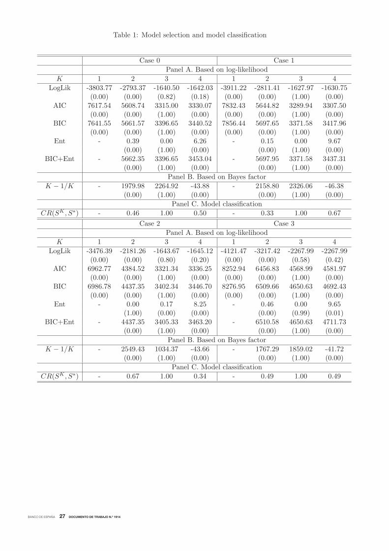
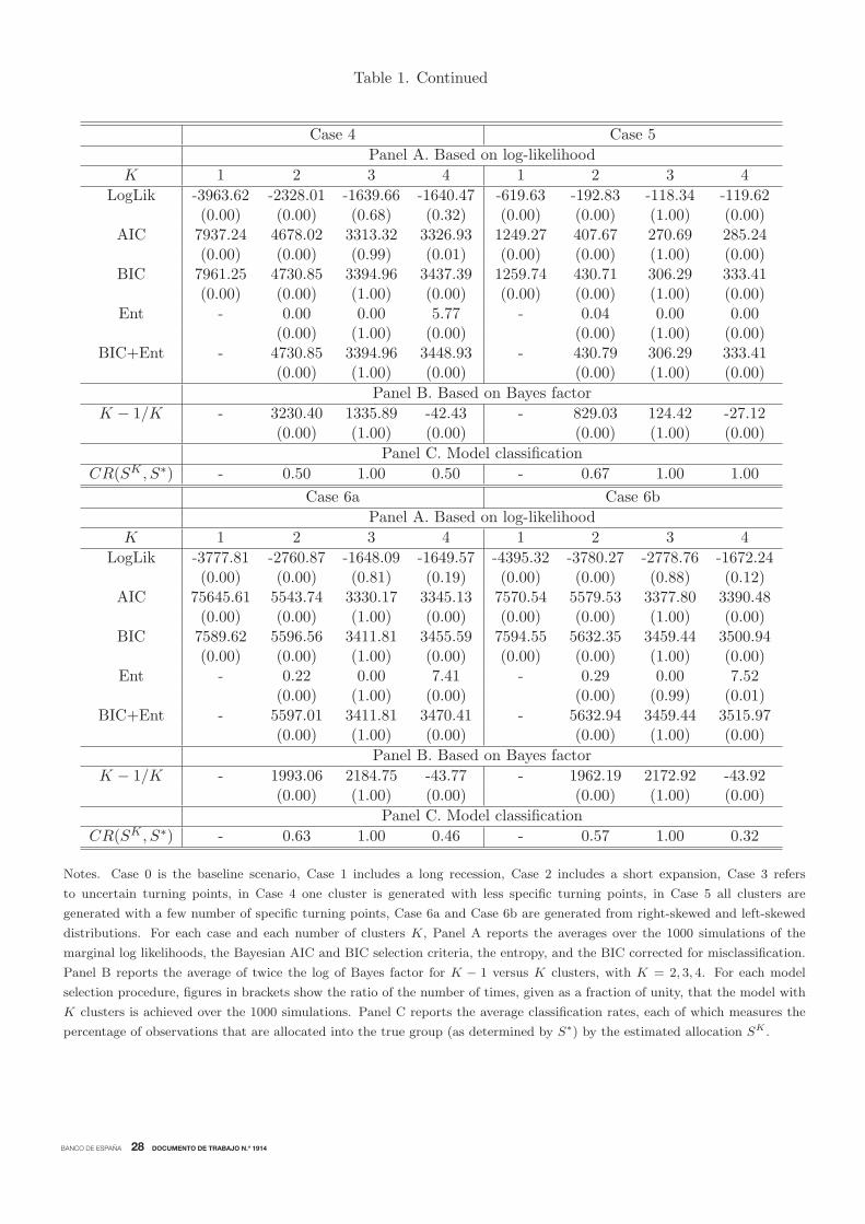
We examine the accuracy of the mixture multiple change-point model approach in grouping the
simulated data set of pairs of specific turning point dates in the correct number of clusters in Table
1. For this purpose, we estimate a set of models MK for K = 1, ....,K∗, with K∗ = 4, and compute
the measures described in Section 2.3 for each K in each of the 1000 simulations from Case 0 to
Case 6b. For each case, the first two panels of the table report the average values of the measures
that determine the number of clusters over the 1000 simulations. In addition, in brackets, the table
shows the ratio of the number of times that the model selection procedure chooses model MK over
the total number of simulations, which estimates the probability that the model selection procedure
chooses K clusters in the mixture model.
The table shows that the measures used to determine the number of clusters unequivocally indi-
cate that the synthetic reference cycle generated in this simulation contains three separate clusters
of pairs of specific turning point dates for each of the cases that we consider in the simulation. For
example, for Case 0, the reported average log value of the estimated marginal likelihood reaches
a maximum of −1640.50 for K = 3 clusters. The averages of AIC, BIC and BIC corrected by
misclassification reach their respective minimums of 3315.00, 3396.65, and 3396.65 also for K = 3
clusters.17
Continuing with Case 0, the average of the entropy associated with the model with three
clusters is zero, indicating a perfect classification of the simulated specific turning points. Finally,
the sequence of averaged (twice the log of) Bayes factors also points toK = 3 because the differences
of the averaged BICs are well above the values that indicate strong evidence for the model with
larger number of clusters for the comparisons of the models with K = 1 versus K = 2 and the
models with K = 2 versus K = 3. However, increasing K from 3 to 4 clusters implies that the
difference of the averaged BICs of the models with K = 3 versus K = 4 is −43.88, which decreases
the averaged odds of a model with K = 4 clusters relative to a model with K = 3 clusters. Notably,
regardless of the model selection procedure, the ratios reported in brackets show that the mixture
model is estimated with the right number of three clusters in all the simulations.18
It is worth pointing out that, although we use Case 0 to describe the table, the accuracy of the
mixture multiple change-point model approaching to determining the correct number of clusters
is consistent regardless of the case being considered. For each of these cases, the model selection
procedures described in this section unambiguously chooses K = 3 clusters even if long recessions,
short expansions, low quality of indicators, low number of indicators, or non-coincident indicators
were involved in the dating procedure.
17Note that BIC coincides with BIC corrected by misclassification for K = 3 because, in this case, the averagedentropy is zero.
18The only exception is the marginal likelihood, which overestimate the number of clusters 18% of the time becausethis method tends to choose models with a large number of components.
which will result in skewness around these clusters of turning points. To examine the effect of
departures from the symmetry implied by the Gaussian mixtures, in Cases 6a and 6b, we simulate
the specific turning points from right-skewed and left-skewed distributions, respectively, by com-
puting a mixture of two distributions. The first one is a normal distribution with the true mean
parameters and the second one is a normal distribution that displaces the mean parameters by -3
months in Case 6a and by +3 months in Case 6b. The proportion of the two distributions is 90%
and 10%, respectively.
3.2 Model selection

BANCO DE ESPAÑA 17 DOCUMENTO DE TRABAJO N.º 1914
where #{s(m)i = k
}counts the number of times that observation i is allocated to cluster k across
the M replications, with k = 1, . . . ,K. A natural classification indicator SK =(sK1 , . . . , sKN
)that
arises from the classification probabilities of a Markov-switching mixture model with K clusters will
associate each observation τi with component k, i.e. sKi = k, if Pr (si = k|θ) reaches a maximum
at k over the K components.
Let S∗ = (s∗1, . . . , s∗N ) be the true allocation of the simulated data. To measure the ability of a
mixture model to assign any specific pair of turning points to the kth group with the classification
indicator SK when it actually arises from that group according to the true classification S∗, we use
where I{sKi =s∗i } takes the value of one whenever observation i is classified by SK in the same cluster
as the true allocation S∗ and zero when this observation is misclassified. Evidently, an allocation
SK with a classification rate of 1 indicates perfect classification because sKi = s∗i for all i = 1, . . . , N .
For each case, the extent to which the selection of the number of clusters in the mixture model
of simulated pairs of turning point dates determines a good partition of the underlying reference
date is examined in the last panel of Table 1. The table reports the average value over the 1000
simulations of the classification rate for various numbers of clusters. For example, in Case 0, when
the number of clusters is under-fitted, which occurs when K = 2, only 46% of the observations are
allocated in the correct cluster. The classification rate of the model with an over-fitted number of
clusters K = 4 is 0.5, indicating that about half of the observations are misclassified. Notably, the
classification rate of the model that correctly uses K = 3 clusters is one, which implies that, on
average, all the observations are allocated correctly.
Again, although we used Case 0 as a basis to describe the results reported in Table 1, a detailed
inspection of this table reveals that all the results obtained for Case 0 are consistent for each of the
cases that we consider in the simulation study. This highlights the valuable ability of the model
to provide an accurate classification of the specific pairs of turning point dates into the different
phases of the reference cycle even when the latter contains double dip recessions, uncertain turning
points, short samples of specific turning points, and asymmetric cycles, which appear when the
disaggregated economic indicators are not coincident.
3.4 Model estimation
In this section, we use the MCMC draws for each of the 1000 simulations for the analysis of the
accuracy of the mixture multiple change-point model to recover the true parameters of the means
and the variances of the K distributions of the mixture.
3.3 Model classification
In addition to model selection, it is worth examining the ability of the Markov-switching mixture
model to provide a posterior classification of the simulated pairs of specific turning point dates into
the different time partitions provided by the reference dates. For this purpose, for each of the 1000
simulations, we estimate the posterior classification probabilities from the 2000 MCMC draws by
the corresponding relative frequency from the retained state draws
Pr (si = k|θ) = 1
M#
{s(m)i = k
}, (17)
the classification rateN
CR(SK , S∗
)=
1
N
N∑i=1
I{sKi =s∗i }, (18)
BANCO DE ESPAÑA 18 DOCUMENTO DE TRABAJO N.º 1914
To check for the accuracy of the model to estimate the means, the first panel of Table 2
shows the Mean Squared Errors (MSE) as the averages over the 1000 simulations of the squared
differences between the posterior means and the true reference dates. Compared to the values
of the true reference dates, which range from 1980 to 2000, the estimated MSE, which range
from 1.50 to 10.17, indicate that the estimated parameter values tend to be very close to the true
parameter values. This high precision in parameter estimation is also observed in the low MSE
in the comparison of the posterior variances and the traces of the covariance matrices and their
respective true values.
Notably, these accurate results are consistent regardless of the case being evaluated, even in
the cases where inference about the reference cycle is computed from a reduced set of coincident
indicators or from a set of low-quality indicators. However, the accuracy in recovering the true
parameters diminishes a bit when the specific reference dates are computed from non-coincident
indicators.
4.1 Dating the historical turning points
The set of disaggregated coincident economic indicators that we use to evaluate the method is
based on the latest available decisions of the NBER Business Cycle Dating Committee about the
timing of the US business cycle turning points. In its most recent memorandum explaining the
June 2009 trough (NBER Business Cycle Dating Committee 2010), the Committee mentions that
it pays particular attention to ten monthly indicators when determining the trough of the Great
Recession in the US reference cycle.19 These indicators are a measure of monthly GDP that has been
developed by the private forecasting firm Macroeconomic Advisers, three measures of monthly GDP
and GDI that have been developed by Stock and Watson (2010b), real manufacturing and trade
sales, industrial production, real personal income excluding transfers, the payroll and household
measures of total employment, and an aggregate of hours of work in the total economy. Although
the number of available observations differs across indicators due to different starting dates and
different release lags, the largest sample spans the period from January 1959 to August 2010, during
which there were eight complete NBER-referenced business cycles.20
The first step of the empirical illustration consists of identifying the individual chronologies of
turning points in each of the ten indicators. To this end, we apply the peak and trough dating algo-
20The Great Recession of 2008 marked the last complete cycle in our sample. Therefore, no further specific turningpoint is detected since then and the sample is still valid to compute historical dates.
19An Excel spreadsheet containing the data for the indicators of economic activity considered by the committee isavailable at
mirror.nber.org/cycles/BCDCFiguresData100920 ver5.xls
The objective of this section is to provide an empirical assessment of the extent to which the
mixture multiple change-point model described in this paper is able to compute accurate inferences
about the reference business cycle turning points in an empirical example with real data. For this
purpose, we focus on the comparison of chronologies of two methods of dating the US reference
cycle: the NBER-referenced business cycle dates, which serves as the standard for accuracy, and
the reference dates obtained from the mixture multiple change-point model.
4 Empirical results
BANCO DE ESPAÑA 19 DOCUMENTO DE TRABAJO N.º 1914
rithm code implemented by Watson (1994), who followed the lines suggested by Bry and Boschan
(1971).21 Figure 1 provides a preliminary inspection of the data by plotting the kernel density
estimator of the bivariate distribution of the resulting pairs of specific peaks and troughs. The
figure reveals that the distribution of turning points is multimodal, exhibiting various modes that
cluster the individual turning points around periods of NBER-referenced recoveries and declines.
The modes of the kernel density of pairs of specific peaks and troughs suggest that the tentative
number of different clusters in the reference cycle could be eight, which correspond with the distinct
local maxima.
To determine the number of clusters formally, we estimate a set of models MK for K =
1, ....,K∗, with K∗ = 9, and compute the measures described in Section 2.3 for each K, whose
21In short, the algorithm isolates local minima and maxima of each of the ten indicators, subject to constraints onboth the length and amplitude of expansions and contractions.
estimates are reported in Table 3. The first column of the table shows that the log of the marginal
likelihood increases uninterruptedly when the number of clusters increases from K = 1 to K = 9,
where it reaches a peak at −53.48. This corresponds with K = 9, although this value is very
close to that obtained for K = 8, −54.33. Although this suggests choosing K = 9, the marginal
likelihood does not take into account the number of parameters in model selection and tends to
overestimate the number of clusters.
Regarding model selection criteria that introduce penalties in model selection, the reported
values in Table 3 of AIC, BIC and BIC corrected by misclassification reach their minimums of
202.66, 297.01, and 297.01, respectively, when K = 8. This indicates that the US reference cycle
requires eight separate cycles. In addition, the entropy of the mixture model with eight clusters
is zero, showing that the model produces a clear segmentation of the reference cycle. Finally, the
sequence of (twice the log of) Bayes factors that compare two models with K − 1 and K different
numbers of clusters, with K = 1, . . . , 9, also points to K = 8. The differences of the BICs are
above the numbers favoring K in the comparison of models with K − 1 versus K clusters, for
K = 1, . . . , 8. However, the difference of the BICs that compares a model with K = 9 versus a
model with K − 1 = 8 becomes negative (−22.25), which supports the conclusion that there is
strong empirical evidence that the number of complete cycles in the US reference cycle from 1959
to 2010 is eight, as the NBER-referenced chronology establishes.
The likelihood-based methods and the entropy measures used to choose the number of clusters
do not reveal which are the parameters that determine the formation of the different clusters and do
not evaluate the extent to which the mixture model provides a good partition of the time span as the
NBER chronology establishes. To examine these questions, we consider sampling representations
from the rejection sampler described in Section 2, which is a very useful tool for visualizing the
posterior mixture distribution. For each of the eight clusters, Figure 2 displays the two-dimensional
scatter plots of the MCMC draws for(μPk , μ
Tk
)in Panel A and for
(μPk ,Σ11,k
)and
(μTk ,Σ22,k
)in
Panel B. From these scatter plots, it is obvious that the component parameters differ mainly in the
means, which present the highest ability to divide the draws into the eight separate groups, whereas
the variances are quite similar for many groups. In addition, Panel A suggests that the clusters of
turning points alternate sequentially, supporting the nonergodic behavior imposed in the transition
matrix to capture the transitions across the distinct business cycles, as a multiple-change model,
which roughly occur about at the NBER-designated turning points.

BANCO DE ESPAÑA 20 DOCUMENTO DE TRABAJO N.º 1914
Figure 3 shows diagnostic plots of the post burn-in draws from the conditional distributions
of μPk , μ
Tk , log (|Σk|) and pk,k and pk,k+1 for each of the K = 8 clusters. These panels help us to
detect potential convergence problems or label switching, which arise when the mixture likelihood
function is not invariant to relabeling the components of a mixture model. The paths of the draws
show that the rejection sampler that imposes, μP (m)k < μ
T (m)k < μ
P (m)k+1 , for all k = 1, . . . ,K, is
useful to prevent label switching because the sampler stays within the modal regions corresponding
to the initial labeling. So, these regions are well separated from the others leading to a unique
labeling.
Table 4 evaluates the mixture multiple change-point model in terms of its capacity to determine
the NBER reference cycle dates. The columns labeled as NBER and MSMM report the reference
22The credible intervals, which range from 0.08 to 1.08 years for peaks and from 0.07 to 1.98 years for troughs,provide a precise estimate of the reference dates.
23The only exception is the 2001 trough, which is located only four months after the NBER dating. The difficultiesof identifying this mild recession have been documented in Kliesen (2003) and Hamilton (2011).
24
Although the ex-post identification of the reference cycle turning points is of great interest in itself,
doing this on an out-of-sample basis is a bigger challenge (Hamilton, 2011). In this section, we
evaluate both the accuracy and the speed with which the mixture multiple change-point model
would have dated the US reference cycle as additional specific cycle turning points were appearing
in (pseudo) real time. Again, the NBER chronology is the basis of comparison.
cycle dates as determined by the NBER and our Markov-Switching Mixture Model. The distinct
means are estimated from the posterior distributions with the help of the rejection Gibbs sampler
algorithm for the mixture model. Using the outputs of the MCMC algorithm, this table also reports,
in brackets, the range of values of the posterior probability distributions that includes 95% of the
probability.22 It is evident that the mixture model replicates the NBER peak and trough dates
very accurately. The method provides exact matches for one peak and three troughs, differing by
less than one quarter either way in the date of the remaining turning points.23 On average, the
method locates the peaks about one and a half months before and the troughs about one sixth of
a month after the NBER dating. Remarkably, there are no instances in which an NBER turning
point date is not matched by a similar date produced by the MSMM model, whose 95% credible
intervals include the NBER-referenced dates in all the episodes.
To provide the results with additional economic meaning, it is worth examining the ability of
the mixture multiple change-point model to provide a posterior classification of the specific turning
point dates into the different business cycles of the US reference cycle. With this aim, we estimate
the posterior classification probabilities Pr (si = k|θ), with k = 1, . . . , 8 and i = 1, . . . , N , from
the MCMC draws through the corresponding relative frequency of the retained state draws, as
described in Section 3. Figure 4, which plots the estimated classification probabilities for each
cluster, shows that the model clearly classifies each specific date, whose classification probabilities
are always close to either 1 or 0. In addition, the probabilities agree with the multiple change-point
behavior of the model, with a large persistence of each state and probabilities that increase nearly
to unity after each structural break that occurs about the turning point dates identified by the
NBER. Thus, the probabilities support the view that the mixture multiple change-point model
performs a segmentation of the time span into non-overlapping business cycle episodes that agrees
with the NBER-referenced cycles.
4.2 Pseudo real-time performance
BANCO DE ESPAÑA 21 DOCUMENTO DE TRABAJO N.º 1914
y g ( ) ( )24Producing real-time vintages is unfeasible because the historical records of some of the ten indicators are not
available.
For this purpose, we use the same data of ten coincident economic indicators described in
the in-sample analysis, which are available from 1959.01 to 2010.08. However, we develop here
a pseudo real-time analysis that consists of computing inferences from successive partitions (one-
month enlargements) of the latest available data set.24 In short, the new information provided by
the ten economic indicators is incorporated into the model month by month as we enlarge the data
set and the model converts the turning point detection into a classification problem. Each month,
the model determines whether the set of incoming specific turning points dates generates a separate
cluster, which would imply that a phase change occurs. To avoid false signals, we follow Chauvet
and Piger (2008) and require that the Bayes factor indicates an increase in the number of clusters
for 3 consecutive months, to confirm that a new reference cycle turning point has appeared. In
addition, since the reference cycle dates are the means of the clusters of the specific dates, we do
not date the new reference turning point until the new specific turning points appear in at least
one-third of the macroeconomic indicators.25
Table 5 evaluates the capacity of the mixture multiple change-point model to date the US
reference cycle in pseudo real time. For a comparative assessment, the left panel reports the NBER
peaks and troughs and the months of their respective announcements, while the right panel displays
the estimated reference cycle turning point chronology produced by the mixture multiple change-
point model and the months when the model detects the phase changes. Using the sample of the
posterior draws, the table reports not only the sample means as point estimates but also the credible
intervals, which are constructed using the 2.5% and 97.5% sample quantiles. Then, comparing
the NBER dates with those established by MSMM measures the accuracy, while comparing the
official months of the announcements with the months in which MSMM identifies the phase changes
quantifies the speed of detection.
The specification whose clusters are determined by Gaussian distributions with means(μPk , μ
Tk
),
the peaks and troughs of the reference cycle, is called peak-trough MSMM. On the other hand,
the model that determines a reference cycle beginning with a trough and whose specific troughs
and peaks are clustered around the means of bivariate Gaussians distributions(μTk , μ
Pk
), is called
trough-peak MSMM. The recursive analysis starts with a vintage of data that covers the period
1959.01-1966.01, which includes one pair of NBER peak-trough dates. Using this sample, we
identify the specific turning points for each indicator by implementing the Bry-Boschan dating
algorithm. Then, we employ the Bayes factor of the peak-trough MSMM model to confirm that
there is only one cluster of specific turning point dates, which is generated from a bivariate normal
density whose means are the first pair of peak-trough reference dates. According to the figures
reported in Figure 5, μP1 and μT
1 are dated in 1960.03 and 1961.02, respectively.
Now, the sample is enlarged by adding one month of observations to each of the ten indicators
and the Bry-Boschan algorithm is re-estimated for the period 1959.01-1966.02. If the outcome of
the dating algorithm does not include any new specific peak, the vintage of data is enlarged again
with the observations of a new month. On the contrary, when a new specific peak is detected by
the Bry-Boschan algorithm, we follow the simple automatic procedure of creating its artificial pair
(trough) by adding the average duration of the preceding recessions to that peak (the preliminary
25Estimating the means with only the early available specific turning points would erroneously produce ex-anteestimates lower than the ex-post estimates.

BANCO DE ESPAÑA 22 DOCUMENTO DE TRABAJO N.º 1914
trough will be replaced by the actual trough as soon as it is detected by Bry-Boschan when new
data arrive). In this way, we increase the sample month by month and estimate the peak-trough
MSMM model with the enlarged outcomes of the Bry-Boschan algorithm. The recursive updated
estimation of the first cluster stops when the Bayes factor that compares the model with K = 1
versus the model with K = 2 indicates that a new cluster has appeared. As Table 5 reports, this
happens in 1971.06 and the peak μP2 is dated in 1969.11.
The procedure described above does not guarantee an accurate estimation of the trough μT2
because it could be partially based on artificial specific troughs. The approach we follow to detect
the following trough is to move to the trough-peak MSMM model as soon as a new peak is detected.
In this case, we omit the peak dated in 1960.03, which converts the reference cycle in a sequence
of clusters centered in pairs of troughs and peaks. Then, the procedure follows the same rules
described above: (i) the sample is updated by one period; (ii) the Bry-Boschan routine is used to
detect new troughs, which are matched up with artificial peaks that guarantee that the current
expansion will last the average of the preceding expansions (replaced by actual peaks when they
appear as the outcome of the Bry-Boschan algorithm); and (iii) the peak-trough MSMM model is
estimated and the Bayes factor that compares the trough-peak MSMM model with K = 1 versus
the model with K = 2 is computed. The automatic procedure continues until K = 2 is preferred
to K = 1, which happens in 1971.06 as reported in Table 5. At this point, we date the trough μT2
in 1970.11 and we move again to the trough-peak MSMM model with the aim of detecting a new
phase change and dating the following peak μP3 .
This automatic procedure goes back and forth from the peak-trough model to the trough-peak
model when new turning points are detected, increasing the sample month by month and applying
the classification procedure provided by MSMM to the enlarged data sets until the end of the
sample in 2010.08. Table 5 examines the success of an analyst who applies MMSM to date the
NBER reference cycle turning point dates in (pseudo) real time each month between 1966.01 and
2010.08, both in terms of timeliness and accuracy. Beginning with the accuracy, the dates assigned
to the reference cycle turning points in pseudo real time are in close agreement to those determined
by the NBER, although the precision of these estimates varies across episodes. The mixture model
produces the same turning points as the NBER in one out of eight peaks and in five out of eight
troughs, and are within a quarter of each other in all but one case. The noticeable exception is
the peak dated in 1989.12 by our method, well before the peak dated in 1990.07 by the NBER,
suggesting that this peak is associated with a leading pattern of some of the coincident indicators.
It is remarkable that the credible intervals contain the NBER dates in all cases.
The following question of interest is the timeliness with which this accurate identification is
achieved. For this purpose, in Table 5 we report the number of months after the NBER turning
point dates that the NBER and MSMM require to identify these turning points. The figures show
a systematic and significant improvement over the NBER in the speed with which business cycle
turning points are identified. On average, MSMM allowed the peaks to be identified 4.4 months
earlier than NBER, and this improvement increases to 11.2 months in the case of troughs. This
improvement over the NBERs business cycle dating committee timeliness when dating the troughs
has been documented by Chauvet and Piger (2008) and Giusto and Piger (2017). Although we were
precluded from using true real time data as they did, we find that MSMM tends to improve the
timeliness of their dating proposals. In addition, MSMM also provides a substantial improvement

BANCO DE ESPAÑA 23 DOCUMENTO DE TRABAJO N.º 1914
in the speed with which the dating methods surveyed by Hamilton (2011) identify the turning
points of the Great Recession.
5 Conclusion
Since the early work of Burns and Mitchell (1946), the reference cycle is viewed as a sequence of
business cycle fluctuations occurring at about the same turning points in many economic activities,
where the dates of the shifts determine the reference dates. However, the fact that the cyclical
turns of different processes are concentrated around certain points in time does not imply that
dating the reference cycle is merely a matter of counting the economic time series that rise and
that fall at about the same time. In fact, dating the reference cycle has been the source of much
debate in both the research literature and policy. The approach pursued in this paper to date the
reference cycle is based on aggregating the specific turning points from a set of coincident economic
indicators.
In our novel proposal, the set of specific turning points dated from a set of coincident indicators
is viewed as a sequence of data with a natural ordering which can be broken down into segments
by the reference cycle turning points. In particular, the specific turning points are supposed to
be drawn from the same Gaussian distribution within each segment, but from different Gaussian
distributions in different segments. Thus, the set of bivariate individual turning points are con-
sidered to arise from a mixture distribution where the different model parameters are assumed to
evolve according to a latent random discrete-state Markov process with the transition probabilities
constrained as in the multiple-change break point model proposed by Chib (1998). In this repre-
sentation, the means of the different Gaussian distributions are viewed as natural estimates of the
reference cycle turning points and the state probabilities are used to determine the change points
of the different reference cycles and to classify the specific turning point dates into the different
business cycles of the reference cycle. In this context, standard Bayesian estimation of finite Markov
mixture modeling techniques is suggested to estimate the model.
The reliability of the proposed framework is validated with simulated data in a Monte Carlo
experiment that try to mimic some stylized facts of business cycle analyses such as short business
cycle phases, uncertain turning points, short samples and specific cycles that come from non-
coincident indicators. The results suggest that the method is very accurate to determine the
number of clusters, to classify the set of specific turning points and to recover the true parameters,
regardless of the stylized business cycle fact being analyzed.
Finally, although the mixture multiple change-point model determines the reference cycle dates
from a set of individual coincident indicators without prior knowledge of any pre-specified dating,
it has been evaluated in terms of its capacity to generate the NBER reference cycle dates. For
this purpose, we use the list of ten coincident indicators employed by the NBER Business Cycle
Committee to determine the trough of the Great Recession. A first benefit of using our method to
determine the historical reference cycle is its replicability. In contrast to the committee approach,
which largely relies on judgment, our automatic method is simple and easy to replicate. Remarkably,
we find that the differences between the ex-post NBER-referenced turning points and the reference
cycle estimated with the mixture multiple change-point model that we propose are almost negligible.
So, it can be used with the aim of performing an ex-post dating the reference cycle of another region
or time.

BANCO DE ESPAÑA 24 DOCUMENTO DE TRABAJO N.º 1914
A second benefit of using our proposal to determine business cycle phase changes is timeliness
because the dating committee announces the turning points with a considerable lag. For example,
the committee announced the December 2007 peak in December 2008 and the June 2009 trough in
September 2010. We evaluate the (pseudo) real-time ability of our proposed algorithm to identify
business cycle turning points in the US economy accurately and in a timely fashion. We find that
our method identifies the dates of the NBER-references turning points very accurately and with a
remarkable speed. Thus, the proposed framework is also a very promising tool for ex-ante detection
and estimation of business cycle turning points.
BANCO DE ESPAÑA 25 DOCUMENTO DE TRABAJO N.º 1914
References
[1] Bensmail, H., Celeux, A., Raftery, E., and Robert, C. 1997. Inference in model-based cluster
analysis. Statistics and Computing 7: 1-10.
[2] Burns, A., Mitchell, W. 1946. Measuring Business Cycles. New York: National Bureau of
Economic Research.
[3] Bry, G., and Boschan, Ch. 1971. Cyclical Analysis of Time Series: Procedures and Computer
Programs. New York: National Bureau of Economic Research.
[4] Business Cycle Dating Committee. 2010. Determination of the June 2009 trough in economic
activity. National Bureau of Economic Research. http://www.nber.org/cycles/sept2010.html.
[5] Celeux, G., Fruhwirth-Schnatter, S., and Robert, C. 2018. Model selection for mixture models.
In G. Celeux, and C. Robert (eds.), Handbook of Mixture Analysis. Boca Raton, FL: CRC
Press.
[6] Chan, J. and Koop, G. 2014. Modelling breaks and clusters in the steady states of macroeco-
nomic variables. Computational Statistics and Data Analysis 76: 186-193.
[7] Chauvet, M., and Piger, J. 2008. A comparison of the real-time performance of business cycle
dating methods. Journal of Business and Economic Statistics 26: 42-49.
[8] Chib, S. 1998. Estimation and comparison of multiple change-point models. Journal of Econo-
metrics 86: 221-241.
[9] Fearnhead, P. 2006. Exact and efficient Bayesian inference for multiple change-point problems.
Statistics and Computing 16: 203-213.
[10] Fraly, Ch. and Raftery, E. 2002. Model-Based Clustering, Discriminant Analysis, and Density
Estimation. Journal of the American Statistical Association 97:458, 611-631.
[11] Fruhwirth-Schnatter, S. 2001. Markov Chain Monte Carlo estimation of classical and dynamic
switching and mixture models. Journal of the American Statistical Association 96: 194-209.
[12] Fruhwirth-Schnatter, S. 2004. Estimating marginal likelihoods for mixture and Markov switch-
ing models using bridge sampling techniques. The Econometrics Journal 7: 143-167.
[13] Fruhwirth-Schnatter, S. 2006. Finite Mixture and Markov Switching models. Springer Series
in Statistics. New York, NY: Springer.
[14] Giordani, P. and Kohn, R. 2008. Efficient Bayesian inference for multiple change-point and
mixture innovation models. Journal of Business and Economic Statistics 26: 66-77.
[15] Giusto, A., and Piger, J. 2017. Identifying business cycle turning points in real time with
vector quantization. International Journal of Forecasting 33: 174-184.
[16] Hamilton, J. 1989. A new approach to the economic analysis of nonstationary time series and
the business cycles. Econometrica 57: 357-384.
BANCO DE ESPAÑA 26 DOCUMENTO DE TRABAJO N.º 1914
[17] Hamilton, J. 2011. Calling recessions in real time. International Journal of Forecasting 27:
1006-1026.
[18] Harding, D., and Pagan, A. 2006. Synchronization of cycles. Journal of Econometrics 132:
59-79.
[19] Harding, D., and Pagan, A. 2016. The econometric analysis of recurrent events in macroeco-
nomics and finance. New Jersey: Princeton University Press.
[20] Kass, R., and Raftery, A. 1995. Bayes factors. Journal of the American Statistical Association
90: 773-795.
[21] Kliesen, K. 2003. The 2001 recession: How was it different and what developments may have
caused it? Federal Reserve Bank of St. Louis Review September/October: 23-37.
[22] Ko, S., Chong, T., and Ghosh P. 2015. Dirichlet process hidden Markov multiple change-point
model. Bayesian Analysis 10: 275-296.
[23] Peluso, S., Chib, S., and Mira, A. 2018. Semiparametric multivariate and multiple change-point
modeling. Bayesian Analysis, forthcoming.
[24] Robert, C. 1996. Mixtures of distributions: Inference and estimation. In W. Gilks, S. Richard-
son, and D. Spiegelhalter (eds.), Markov Chain Monte Carlo in practice. London: Chapman
and Hall.
[25] Stock, J., and Watson, M. 2010a. Indicators for dating business cycles: cross-history selection
and comparisons. American Economic Review: Papers and Proceedings 100: 16-19.
[26] Stock, J., and Watson, M. 2010b. New Indexes of Monthly GDP, available at
http://www.princeton.edu/˜ mwatson/mgdp gdi.html.
[27] Stock, J., and Watson, M. 2014. Estimating turning points using large data sets. Journal of
Econometrics 178: 368-381.
[28] Watson, M. 1994. Business-cycle durations and postwar stabilization of the US economy. Amer-
ican Economic Review 84: 24-46.
BANCO DE ESPAÑA 27 DOCUMENTO DE TRABAJO N.º 1914
Table 1: Model selection and model classification
Case 0 Case 1
Panel A. Based on log-likelihood
K 1 2 3 4 1 2 3 4
LogLik -3803.77 -2793.37 -1640.50 -1642.03 -3911.22 -2811.41 -1627.97 -1630.75(0.00) (0.00) (0.82) (0.18) (0.00) (0.00) (1.00) (0.00)
AIC 7617.54 5608.74 3315.00 3330.07 7832.43 5644.82 3289.94 3307.50(0.00) (0.00) (1.00) (0.00) (0.00) (0.00) (1.00) (0.00)
BIC 7641.55 5661.57 3396.65 3440.52 7856.44 5697.65 3371.58 3417.96(0.00) (0.00) (1.00) (0.00) (0.00) (0.00) (1.00) (0.00)
Ent - 0.39 0.00 6.26 - 0.15 0.00 9.67(0.00) (1.00) (0.00) (0.00) (1.00) (0.00)
BIC+Ent - 5662.35 3396.65 3453.04 - 5697.95 3371.58 3437.31(0.00) (1.00) (0.00) (0.00) (1.00) (0.00)
Panel B. Based on Bayes factor
K − 1/K - 1979.98 2264.92 -43.88 - 2158.80 2326.06 -46.38(0.00) (1.00) (0.00) (0.00) (1.00) (0.00)
Panel C. Model classification
CR(SK , S∗) - 0.46 1.00 0.50 - 0.33 1.00 0.67
Case 2 Case 3
Panel A. Based on log-likelihood
K 1 2 3 4 1 2 3 4
LogLik -3476.39 -2181.26 -1643.67 -1645.12 -4121.47 -3217.42 -2267.99 -2267.99(0.00) (0.00) (0.80) (0.20) (0.00) (0.00) (0.58) (0.42)
AIC 6962.77 4384.52 3321.34 3336.25 8252.94 6456.83 4568.99 4581.97(0.00) (0.00) (1.00) (0.00) (0.00) (0.00) (1.00) (0.00)
BIC 6986.78 4437.35 3402.34 3446.70 8276.95 6509.66 4650.63 4692.43(0.00) (0.00) (1.00) (0.00) (0.00) (0.00) (1.00) (0.00)
Ent - 0.00 0.17 8.25 - 0.46 0.00 9.65(1.00) (0.00) (0.00) (0.00) (0.99) (0.01)
BIC+Ent - 4437.35 3405.33 3463.20 - 6510.58 4650.63 4711.73(0.00) (1.00) (0.00) (0.00) (1.00) (0.00)
Panel B. Based on Bayes factor
K − 1/K - 2549.43 1034.37 -43.66 - 1767.29 1859.02 -41.72(0.00) (1.00) (0.00) (0.00) (1.00) (0.00)
Panel C. Model classification
CR(SK , S∗) - 0.67 1.00 0.34 - 0.49 1.00 0.49
BANCO DE ESPAÑA 28 DOCUMENTO DE TRABAJO N.º 1914
Table 1. Continued
Case 4 Case 5
Panel A. Based on log-likelihood
K 1 2 3 4 1 2 3 4
LogLik -3963.62 -2328.01 -1639.66 -1640.47 -619.63 -192.83 -118.34 -119.62(0.00) (0.00) (0.68) (0.32) (0.00) (0.00) (1.00) (0.00)
AIC 7937.24 4678.02 3313.32 3326.93 1249.27 407.67 270.69 285.24(0.00) (0.00) (0.99) (0.01) (0.00) (0.00) (1.00) (0.00)
BIC 7961.25 4730.85 3394.96 3437.39 1259.74 430.71 306.29 333.41(0.00) (0.00) (1.00) (0.00) (0.00) (0.00) (1.00) (0.00)
Ent - 0.00 0.00 5.77 - 0.04 0.00 0.00(0.00) (1.00) (0.00) (0.00) (1.00) (0.00)
BIC+Ent - 4730.85 3394.96 3448.93 - 430.79 306.29 333.41(0.00) (1.00) (0.00) (0.00) (1.00) (0.00)
Panel B. Based on Bayes factor
K − 1/K - 3230.40 1335.89 -42.43 - 829.03 124.42 -27.12(0.00) (1.00) (0.00) (0.00) (1.00) (0.00)
Panel C. Model classification
CR(SK , S∗) - 0.50 1.00 0.50 - 0.67 1.00 1.00
Case 6a Case 6b
Panel A. Based on log-likelihood
K 1 2 3 4 1 2 3 4
LogLik -3777.81 -2760.87 -1648.09 -1649.57 -4395.32 -3780.27 -2778.76 -1672.24(0.00) (0.00) (0.81) (0.19) (0.00) (0.00) (0.88) (0.12)
AIC 75645.61 5543.74 3330.17 3345.13 7570.54 5579.53 3377.80 3390.48(0.00) (0.00) (1.00) (0.00) (0.00) (0.00) (1.00) (0.00)
BIC 7589.62 5596.56 3411.81 3455.59 7594.55 5632.35 3459.44 3500.94(0.00) (0.00) (1.00) (0.00) (0.00) (0.00) (1.00) (0.00)
Ent - 0.22 0.00 7.41 - 0.29 0.00 7.52(0.00) (1.00) (0.00) (0.00) (0.99) (0.01)
BIC+Ent - 5597.01 3411.81 3470.41 - 5632.94 3459.44 3515.97(0.00) (1.00) (0.00) (0.00) (1.00) (0.00)
Panel B. Based on Bayes factor
K − 1/K - 1993.06 2184.75 -43.77 - 1962.19 2172.92 -43.92(0.00) (1.00) (0.00) (0.00) (1.00) (0.00)
Panel C. Model classification
CR(SK , S∗) - 0.63 1.00 0.46 - 0.57 1.00 0.32
Notes. Case 0 is the baseline scenario, Case 1 includes a long recession, Case 2 includes a short expansion, Case 3 refers
to uncertain turning points, in Case 4 one cluster is generated with less specific turning points, in Case 5 all clusters are
generated with a few number of specific turning points, Case 6a and Case 6b are generated from right-skewed and left-skewed
distributions. For each case and each number of clusters K, Panel A reports the averages over the 1000 simulations of the
marginal log likelihoods, the Bayesian AIC and BIC selection criteria, the entropy, and the BIC corrected for misclassification.
Panel B reports the average of twice the log of Bayes factor for K − 1 versus K clusters, with K = 2, 3, 4. For each model
selection procedure, figures in brackets show the ratio of the number of times, given as a fraction of unity, that the model with
K clusters is achieved over the 1000 simulations. Panel C reports the average classification rates, each of which measures the
percentage of observations that are allocated into the true group (as determined by S∗) by the estimated allocation SK .
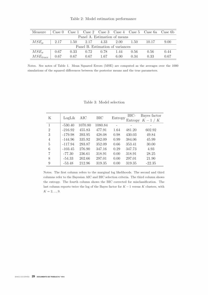
BANCO DE ESPAÑA 29 DOCUMENTO DE TRABAJO N.º 1914
Table 2: Model estimation performance
Measure Case 0 Case 1 Case 2 Case 3 Case 4 Case 5 Case 6a Case 6b
Panel A. Estimation of means
MSEμ 2.17 1.50 2.17 4.33 2.00 1.50 10.17 9.00
Panel B. Estimation of variances
MSEσ 0.67 0.33 0.72 0.78 1.44 0.56 0.56 0.44MSEtrace 0.67 0.67 0.67 1.67 6.00 0.34 0.33 0.67
Notes. See notes of Table 1. Mean Squared Errors (MSE) are computed as the averages over the 1000
simulations of the squared differences between the posterior means and the true parameters.
Table 3: Model selection
K LogLik AIC BIC EntropyBIC-Entropy
Bayes factorK − 1 / K
1 -530.40 1070.80 1080.84 - - -2 -216.92 455.83 477.91 1.64 481.20 602.923 -179.98 393.95 428.08 0.98 430.03 49.844 -144.96 335.92 382.09 0.99 384.06 45.995 -117.94 293.87 352.09 0.66 353.41 30.006 -103.45 276.90 347.16 0.29 347.73 4.937 -77.30 236.61 318.91 0.00 318.91 28.258 -54.33 202.66 297.01 0.00 297.01 21.909 -53.48 212.96 319.35 0.00 319.35 -22.35
Notes. The first column refers to the marginal log likelihoods. The second and third
columns refer to the Bayesian AIC and BIC selection criteria. The third column shows
the entropy. The fourth column shows the BIC corrected for misclassification. The
last column reports twice the log of the Bayes factor for K − 1 versus K clusters, with
K = 2, ..., 9.
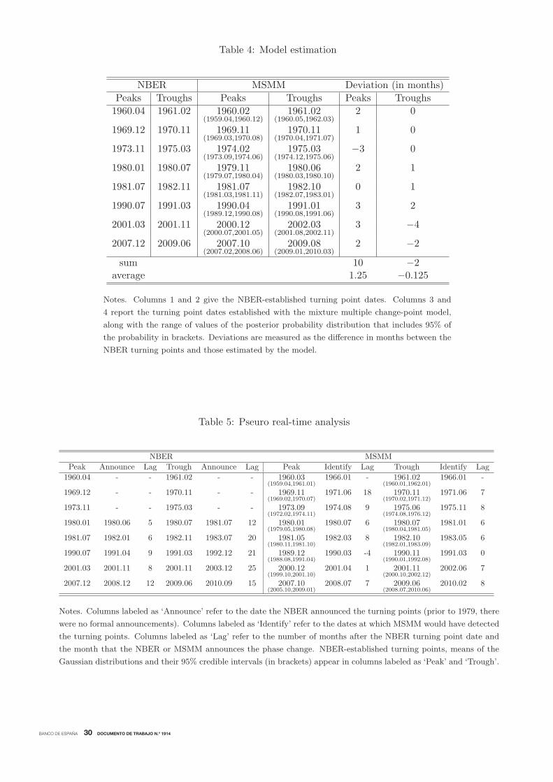
BANCO DE ESPAÑA 30 DOCUMENTO DE TRABAJO N.º 1914
Table 4: Model estimation
NBER MSMM Deviation (in months)
Peaks Troughs Peaks Troughs Peaks Troughs
1960.04 1961.02 1960.02(1959.04,1960.12)
1961.02(1960.05,1962.03)
2 0
1969.12 1970.11 1969.11(1969.03,1970.08)
1970.11(1970.04,1971.07)
1 0
1973.11 1975.03 1974.02(1973.09,1974.06)
1975.03(1974.12,1975.06)
−3 0
1980.01 1980.07 1979.11(1979.07,1980.04)
1980.06(1980.03,1980.10)
2 1
1981.07 1982.11 1981.07(1981.03,1981.11)
1982.10(1982.07,1983.01)
0 1
1990.07 1991.03 1990.04(1989.12,1990.08)
1991.01(1990.08,1991.06)
3 2
2001.03 2001.11 2000.12(2000.07,2001.05)
2002.03(2001.08,2002.11)
3 −42007.12 2009.06 2007.10
(2007.02,2008.06)2009.08
(2009.01,2010.03)2 −2
sum 10 −2average 1.25 −0.125
Notes. Columns 1 and 2 give the NBER-established turning point dates. Columns 3 and
4 report the turning point dates established with the mixture multiple change-point model,
along with the range of values of the posterior probability distribution that includes 95% of
the probability in brackets. Deviations are measured as the difference in months between the
NBER turning points and those estimated by the model.
Table 5: Pseuro real-time analysis
NBER MSMM
Peak Announce Lag Trough Announce Lag Peak Identify Lag Trough Identify Lag
1960.04 - - 1961.02 - - 1960.03(1959.04,1961.01)
1966.01 - 1961.02(1960.01,1962.01)
1966.01 -
1969.12 - - 1970.11 - - 1969.11(1969.02,1970.07)
1971.06 18 1970.11(1970.02,1971.12)
1971.06 7
1973.11 - - 1975.03 - - 1973.09(1972.02,1974.11)
1974.08 9 1975.06(1974.08,1976.12)
1975.11 8
1980.01 1980.06 5 1980.07 1981.07 12 1980.01(1979.05,1980.08)
1980.07 6 1980.07(1980.04,1981.05)
1981.01 6
1981.07 1982.01 6 1982.11 1983.07 20 1981.05(1980.11,1981.10)
1982.03 8 1982.10(1982.01,1983.09)
1983.05 6
1990.07 1991.04 9 1991.03 1992.12 21 1989.12(1988.08,1991.04)
1990.03 -4 1990.11(1990.01,1992.08)
1991.03 0
2001.03 2001.11 8 2001.11 2003.12 25 2000.12(1999.10,2001.10)
2001.04 1 2001.11(2000.10,2002.12)
2002.06 7
2007.12 2008.12 12 2009.06 2010.09 15 2007.10(2005.10,2009.01)
2008.07 7 2009.06(2008.07,2010.06)
2010.02 8
Notes. Columns labeled as ‘Announce’ refer to the date the NBER announced the turning points (prior to 1979, there
were no formal announcements). Columns labeled as ‘Identify’ refer to the dates at which MSMM would have detected
the turning points. Columns labeled as ‘Lag’ refer to the number of months after the NBER turning point date and
the month that the NBER or MSMM announces the phase change. NBER-established turning points, means of the
Gaussian distributions and their 95% credible intervals (in brackets) appear in columns labeled as ‘Peak’ and ‘Trough’.
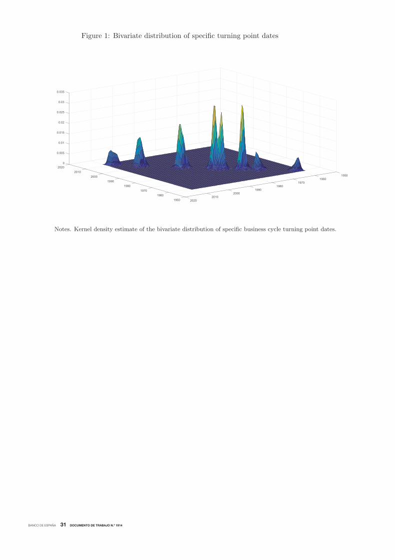
BANCO DE ESPAÑA 31 DOCUMENTO DE TRABAJO N.º 1914
Figure 1: Bivariate distribution of specific turning point dates
02020
0.005
0.01
2010
0.015
19502000
0.02
19601990
0.025
1970
0.03
1980 1980
0.035
1990197020001960 2010
1950 2020
Notes. Kernel density estimate of the bivariate distribution of specific business cycle turning point dates.
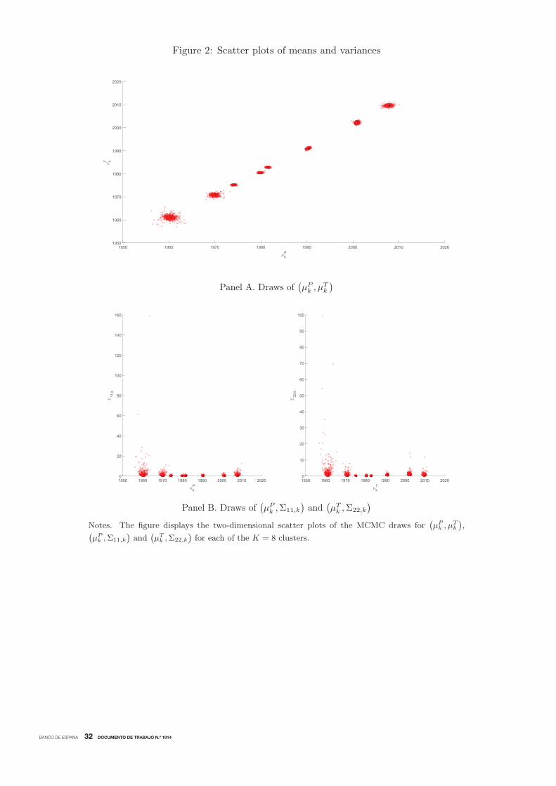
BANCO DE ESPAÑA 32 DOCUMENTO DE TRABAJO N.º 1914
Figure 2: Scatter plots of means and variances
1950 1960 1970 1980 1990 2000 2010 2020
μkP
1950
1960
1970
1980
1990
2000
2010
2020
μkT
1
2
3
4
5
6
7
8
Panel A. Draws of(μPk , μ
Tk
)
1950 1960 1970 1980 1990 2000 2010 2020
μkP
0
20
40
60
80
100
120
140
160
Σ11,k
1 2 3 4 5 6 7 8
1950 1960 1970 1980 1990 2000 2010 2020
μkT
0
10
20
30
40
50
60
70
80
90
100
Σ22,k
1 2 3 4 5 6 7 8
Panel B. Draws of(μPk ,Σ11,k
)and
(μTk ,Σ22,k
)Notes. The figure displays the two-dimensional scatter plots of the MCMC draws for
(μPk , μ
Tk
),
(μPk ,Σ11,k
)and
(μTk ,Σ22,k
)for each of the K = 8 clusters.
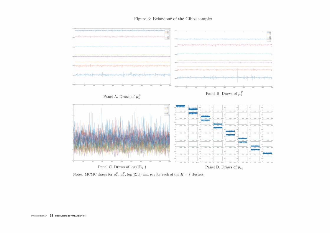
BANCO DE ESPAÑA 33 DOCUMENTO DE TRABAJO N.º 1914
Figure 3: Behaviour of the Gibbs sampler
0 200 400 600 800 1000 1200 1400 1600 1800 20001950
1960
1970
1980
1990
2000
2010k=1k=2k=3k=4k=5k=6k=7k=8
Panel A. Draws of μPk
0 200 400 600 800 1000 1200 1400 1600 1800 20001950
1960
1970
1980
1990
2000
2010
2020k=1k=2k=3k=4k=5k=6k=7k=8
Panel B. Draws of μTk
0 200 400 600 800 1000 1200 1400 1600 1800 2000-6
-5
-4
-3
-2
-1
0
1
2
3
4k=1k=2k=3k=4k=5k=6k=7k=8
Panel C. Draws of log (|Σk|) Panel D. Draws of pi,j
Notes. MCMC draws for μPk , μ
Tk , log (|Σk|) and pi,j for each of the K = 8 clusters.
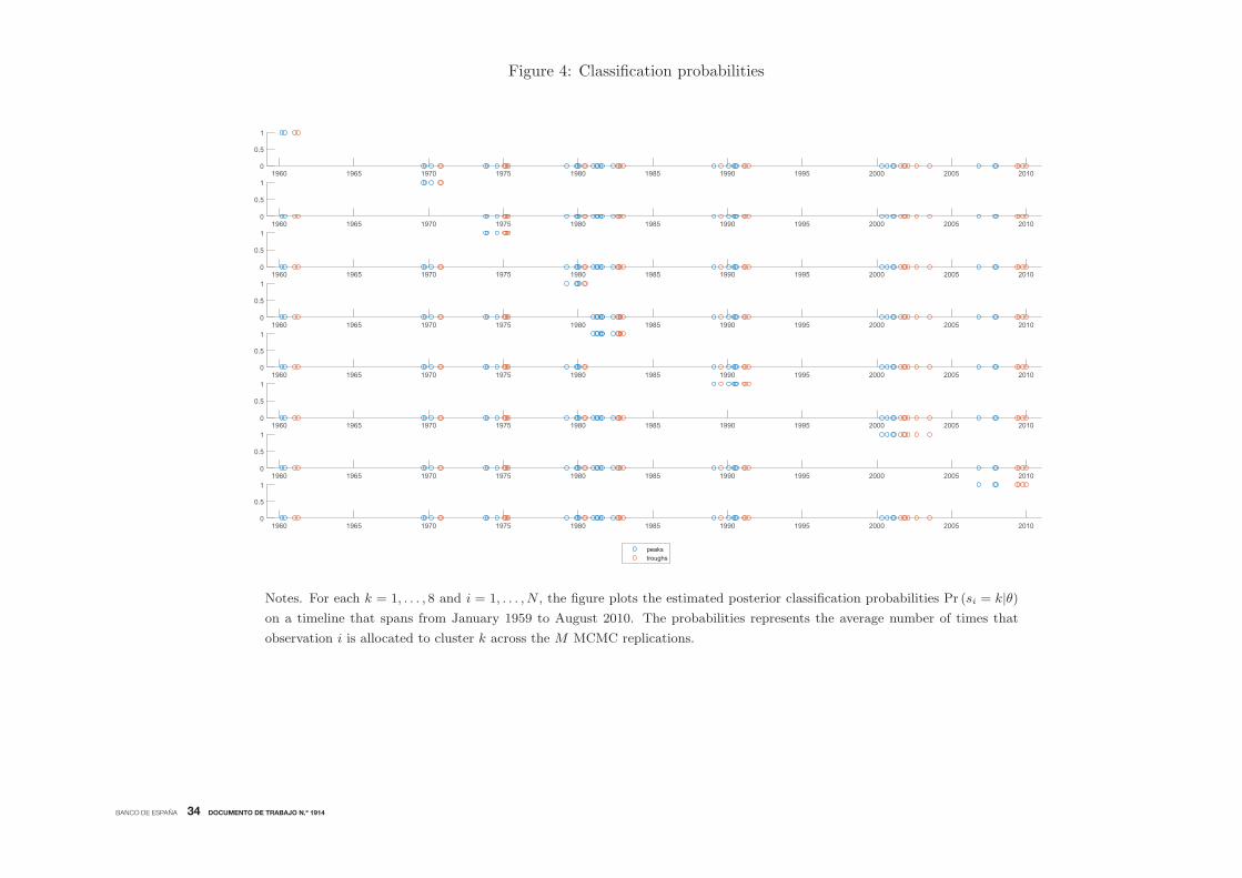
BANCO DE ESPAÑA 34 DOCUMENTO DE TRABAJO N.º 1914
Figure 4: Classification probabilities
1960 1965 1970 1975 1980 1985 1990 1995 2000 2005 20100
0.5
1
1960 1965 1970 1975 1980 1985 1990 1995 2000 2005 20100
0.5
1
1960 1965 1970 1975 1980 1985 1990 1995 2000 2005 20100
0.5
1
1960 1965 1970 1975 1980 1985 1990 1995 2000 2005 20100
0.5
1
1960 1965 1970 1975 1980 1985 1990 1995 2000 2005 20100
0.5
1
1960 1965 1970 1975 1980 1985 1990 1995 2000 2005 20100
0.5
1
1960 1965 1970 1975 1980 1985 1990 1995 2000 2005 20100
0.5
1
1960 1965 1970 1975 1980 1985 1990 1995 2000 2005 20100
0.5
1
peakstroughs
Notes. For each k = 1, . . . , 8 and i = 1, . . . , N , the figure plots the estimated posterior classification probabilities Pr (si = k|θ)on a timeline that spans from January 1959 to August 2010. The probabilities represents the average number of times that
observation i is allocated to cluster k across the M MCMC replications.
BANCO DE ESPAÑA PUBLICATIONS
WORKING PAPERS
1820 MARIO ALLOZA, PABLO BURRIEL and JAVIER J. PÉREZ: Fiscal policies in the euro area: revisiting the size of
spillovers.
1821 MARTA MARTÍNEZ-MATUTE and ALBERTO URTASUN: Uncertainty, fi rm heterogeneity and labour adjustments.
Evidence from European countries.
1822 GABRIELE FIORENTINI, ALESSANDRO GALESI, GABRIEL PÉREZ-QUIRÓS and ENRIQUE SENTANA: The rise and fall
of the natural interest rate.
1823 ALBERTO MARTÍN, ENRIQUE MORAL-BENITO and TOM SCHMITZ: The fi nancial transmission of housing bubbles:
evidence from Spain.
1824 DOMINIK THALER: Sovereign default, domestic banks and exclusion from international capital markets.
1825 JORGE E. GALÁN and JAVIER MENCÍA: Empirical assessment of alternative structural methods for identifying cyclical
systemic risk in Europe.
1826 ROBERTO BLANCO and NOELIA JIMÉNEZ: Credit allocation along the business cycle: evidence from the latest boom
bust credit cycle in Spain.
1827 ISABEL ARGIMÓN: The relevance of currency-denomination for the cross-border effects of monetary policy.
1828 SANDRA GARCÍA-URIBE: The effects of tax changes on economic activity: a narrative approach to frequent
anticipations.
1829 MATÍAS CABRERA, GERALD P. DWYER and MARÍA J. NIETO: The G-20 regulatory agenda and bank risk.
1830 JACOPO TIMINI and MARINA CONESA: Chinese exports and non-tariff measures: testing for heterogeneous effects at the
product level.
1831 JAVIER ANDRÉS, JOSÉ E. BOSCÁ, JAVIER FERRI and CRISTINA FUENTES-ALBERO: Households’ balance sheets and
the effect of fi scal policy.
1832 ÓSCAR ARCE, MIGUEL GARCÍA-POSADA, SERGIO MAYORDOMO and STEVEN ONGENA: Adapting lending policies
when negative interest rates hit banks’ profi ts.
1833 VICENTE SALAS, LUCIO SAN JUAN and JAVIER VALLÉS: Corporate cost and profi t shares in the euro area and the US:
the same story?
1834 MARTÍN GONZÁLEZ-EIRAS and CARLOS SANZ: Women’s representation in politics: voter bias, party bias, and electoral
systems.
1835 MÓNICA CORREA-LÓPEZ and BEATRIZ DE BLAS: Faraway, so close! Technology diffusion and fi rm heterogeneity in the
medium term cycle of advanced economies.
1836 JACOPO TIMINI: The margins of trade: market entry and sector spillovers, the case of Italy (1862-1913).
1837 HENRIQUE S. BASSO and OMAR RACHEDI: The young, the old, and the government: demographics and fi scal
multipliers.
1838 PAU ROLDÁN and SONIA GILBUKH: Firm dynamics and pricing under customer capital accumulation.
1839 GUILHERME BANDEIRA, JORDI CABALLÉ and EUGENIA VELLA: Should I stay or should I go? Austerity,
unemployment and migration.
1840 ALESSIO MORO and OMAR RACHEDI: The changing structure of government consumption spending.
1841 GERGELY GANICS, ATSUSHI INOUE and BARBARA ROSSI: Confi dence intervals for bias and size distortion in IV
and local projections – IV models.
1842 MARÍA GIL, JAVIER J. PÉREZ, A. JESÚS SÁNCHEZ and ALBERTO URTASUN: Nowcasting private consumption:
traditional indicators, uncertainty measures, credit cards and some internet data.
1843 MATÍAS LAMAS and JAVIER MENCÍA: What drives sovereign debt portfolios of banks in a crisis context?
1844 MIGUEL ALMUNIA, POL ANTRÀS, DAVID LÓPEZ-RODRÍGUEZ and EDUARDO MORALES: Venting out: exports during
a domestic slump.
1845 LUCA FORNARO and FEDERICA ROMEI: The paradox of global thrift.
1846 JUAN S. MORA-SANGUINETTI and MARTA MARTÍNEZ-MATUTE: An economic analysis of court fees: evidence from
the Spanish civil jurisdiction.
1847 MIKEL BEDAYO, ÁNGEL ESTRADA and JESÚS SAURINA: Bank capital, lending booms, and busts. Evidence from
Spain in the last 150 years.
1848 DANIEL DEJUÁN and CORINNA GHIRELLI: Policy uncertainty and investment in Spain.
1849 CRISTINA BARCELÓ and ERNESTO VILLANUEVA: The risk of job loss, household formation and housing demand:
evidence from differences in severance payments.
1850 FEDERICO TAGLIATI: Welfare effects of an in-kind transfer program: evidence from Mexico.
1851 ÓSCAR ARCE, GALO NUÑO, DOMINIK THALER and CARLOS THOMAS: A large central bank balance sheet? Floor vs
corridor systems in a New Keynesian environment.
1901 EDUARDO GUTIÉRREZ and ENRIQUE MORAL-BENITO: Trade and credit: revisiting the evidence.
1902 LAURENT CAVENAILE and PAU ROLDAN: Advertising, innovation and economic growth.
1903 DESISLAVA C. ANDREEVA and MIGUEL GARCÍA-POSADA: The impact of the ECB’s targeted long-term refi nancing
operations on banks’ lending policies: the role of competition.
1904 ANDREA ALBANESE, CORINNA GHIRELLI and MATTEO PICCHIO: Timed to say goodbye: does unemployment
benefi t eligibility affect worker layoffs?
1905 CORINNA GHIRELLI, MARÍA GIL, JAVIER J. PÉREZ and ALBERTO URTASUN: Measuring economic and economic
policy uncertainty, and their macroeconomic effects: the case of Spain.
1906 CORINNA GHIRELLI, JAVIER J. PÉREZ and ALBERTO URTASUN: A new economic policy uncertainty index for Spain.
1907 ESTEBAN GARCÍA-MIRALLES, NEZIH GUNER and ROBERTO RAMOS: The Spanish personal income tax:
facts and parametric estimates.
1908 SERGIO MAYORDOMO and OMAR RACHEDI: The China syndrome affects banks: the credit supply channel of
foreign import competition.
1909 MÓNICA CORREA-LÓPEZ, MATÍAS PACCE and KATHI SCHLEPPER: Exploring trend infl ation dynamics in Euro Area
countries.
1910 JAMES COSTAIN, ANTON NAKOV and BORJA PETIT: Monetary policy implications of state-dependent prices and wages.
1911 JAMES CLOYNE, CLODOMIRO FERREIRA, MAREN FROEMEL and PAOLO SURICO: Monetary policy, corporate
fi nance and investment.
1912 CHRISTIAN CASTRO and JORGE E. GALÁN: Drivers of productivity in the Spanish banking sector: recent evidence.
1913 SUSANA PÁRRAGA RODRÍGUEZ: The effects of pension-related policies on household spending.
1914 MÁXIMO CAMACHO, MARÍA DOLORES GADEA and ANA GÓMEZ LOSCOS: A new approach to dating the reference
cycle.
Unidad de Servicios AuxiliaresAlcalá, 48 - 28014 Madrid
E-mail: [email protected]