Embed Size (px)
Citation preview
Rev Deriv Res (2007) 10:87–150DOI 10.1007/s11147-007-9014-6
A new approach for option pricing under stochasticvolatility
Peter Carr · Jian Sun
Published online: 20 February 2008© Springer Science+Business Media, LLC 2008
Abstract We develop a new approach for pricing European-style contingent claimswritten on the time T spot price of an underlying asset whose volatility is stochastic.Like most of the stochastic volatility literature, we assume continuous dynamics forthe price of the underlying asset. In contrast to most of the stochastic volatility liter-ature, we do not directly model the dynamics of the instantaneous volatility. Instead,taking advantage of the recent rise of the variance swap market, we directly assumecontinuous dynamics for the time T variance swap rate. The initial value of this var-iance swap rate can either be directly observed, or inferred from option prices. Wemake no assumption concerning the real world drift of this process. We assume thatthe ratio of the volatility of the variance swap rate to the instantaneous volatility ofthe underlying asset just depends on the variance swap rate and on the variance swapmaturity. Since this ratio is assumed to be independent of calendar time, we term thiskey assumption the stationary volatility ratio hypothesis (SVRH). The instantaneousvolatility of the futures follows an unspecified stochastic process, so both the under-lying futures price and the variance swap rate have unspecified stochastic volatility.Despite this, we show that the payoff to a path-independent contingent claim can beperfectly replicated by dynamic trading in futures contracts and variance swaps ofthe same maturity. As a result, the contingent claim is uniquely valued relative to itsunderlying’s futures price and the assumed observable variance swap rate. In contrastto standard models of stochastic volatility, our approach does not require specifying themarket price of volatility risk or observing the initial level of instantaneous volatility.
P. Carr (B)Bloomberg LP, 731 Lexington Avenue, New York, NY 10022, USAe-mail: [email protected]
J. SunXE Capital Management, 24 West 40th Street, New York, NY 10018, USAe-mail: [email protected]
123
88 P. Carr, J. Sun
As a consequence of our SVRH, the partial differential equation (PDE) governing thearbitrage-free value of the contingent claim just depends on two state variables ratherthan the usual three. We then focus on the consistency of our SVRH with the standardassumption that the risk-neutral process for the instantaneous variance is a diffusionwhose coefficients are independent of the variance swap maturity. We show that thecombination of this maturity independent diffusion hypothesis (MIDH) and our SVRHimplies a very special form of the risk-neutral diffusion process for the instantaneousvariance. Fortunately, this process is tractable, well-behaved, and enjoys empiricalsupport. Finally, we show that our model can also be used to robustly price and hedgevolatility derivatives.
Keywords Option pricing · Stochastic volatility
1 Introduction
In this article, we consider the standard problem of valuing and hedging a contin-gent claim written on the price at expiry of some underlying asset. In contrast tothe standard model of Black and Scholes (1973) and Merton (1973), we assume thatboth the spot price and the instantaneous volatility of the claim’s underlying asset arestochastic and imperfectly correlated. The standard approach to derivative securityvaluation under stochastic volatility specifies the statistical dynamics and derives therisk-neutral dynamics of both quantities. As is well known, this approach requiresspecifying the market price of volatility risk. This specification is fraught with diffi-culty since this market price is not directly observable. Even if one manages to achievethe correct parametrization of the market price of volatility risk, the identification ofthese parameters and the initial instantaneous volatility from option prices can beproblematic in practice.
Fortunately, there is an alternative approach which bypasses the need to specify thedynamics of the market price of volatility risk. It also bypasses the need to observeor infer the instantaneous volatility. The approach is to model the statistical dynamicsof some process which is a known function of option prices. As the instantaneousvolatility of the underlying asset is intrinsic to option valuation, this function shouldhave the property that this instantaneous volatility can be expressed in terms of thisprocess. Since the risk-neutral relative drift of an option price is just the riskfree rate,the risk-neutral drift of the process can be calculated through Itô’s formula. If the sta-tistical process describing the function of options prices is assumed to be continuousover time, then all that remains is to model the statistical volatility of the process.
This approach was pioneered in Dupire (1992). Inspired by the pioneering contri-bution of Heath et al. (1992) to the analysis of interest rate derivatives, the functionof the option prices which Dupire chose was the entire term structure of forwardvariance swap rates. Assuming only positivity and continuity of the underlying assetprice, Dupire showed that a forward variance swap rate can be determined from thecost of forming a particular static position in options involving a continuum of strikeprices. As a result, the risk-neutral drift of the forward variance swap rate is zero. Once
123
A new approach for option pricing 89
one specifies the volatility of all forward variance swap rates, one also determines therisk-neutral dynamics of the instantaneous variance of the underlying.
Unfortunately, the determination of the initial curve of forward variance swap ratescan be tricky in practice due to the discreteness of strikes and maturities in optionsmarkets. Now that variance swaps trade outright, one can overcome the discrete strikesissue by direct observation of variance swap rates. However, the discreteness of matu-rities in the relatively nascent variance swap market still makes observation of theinitial continuum of variance swap rates tricky in practice.
To circumvent this problem, Duanmu (2004) proposes modelling the spot varianceswap rate of a single maturity.1 He assumes a particular diffusion process for the vari-ance swap rate and shows that the payoff to volatility derivatives of the same maturitycan be replicated by dynamic trading in variance swaps.
Like Duanmu, Potter (2004) also proposes completing markets by dynamic tradingin variance swaps of a single maturity. Like us, Potter examines the implications ofthis assumption for the valuation of contingent claims on price as well as for volatilityderivatives. To value these claims, he assumes that the instantaneous variance of theunderlying asset is an affine function of the variance swap rate. He then shows that thisassumption is a consequence of the dynamics assumed in several popular stochasticvolatility models. He also analyzes Duanmu’s model and shows that it is a special caseof his framework in which the instantaneous variance of the underlying asset is justthe variance swap rate.
Our analysis is similar to that of Duanmu and Potter in that we model the dynamicsof a variance swap rate of a single maturity. Like them and Dupire, we do not have tospecify the market price of volatility risk. The major difference between our work andall previous work is that we impose a special structure on the assumed dynamics ofthe variance swap rate. In particular, we assume that the ratio of the volatility of thevariance swap rate to the instantaneous volatility of the underlying asset just dependson the variance swap rate and the variance swap maturity. Since this ratio is assumed tobe independent of calendar time, we term this key assumption the stationary volatilityratio hypothesis (SVRH).
The instantaneous volatility of the futures follows an unspecified stochastic pro-cess, so both the underlying futures price and the variance swap rate have unspecifiedstochastic volatility. Despite this, we show that the payoff to a path-independent con-tingent claim can be perfectly replicated by dynamic trading in futures contracts andvariance swaps of the same maturity. As a result, no arbitrage implies that the contin-gent claim is uniquely valued relative to its underlying’s futures price and the assumedobservable variance swap rate. Under the SVRH, parsimony is achieved in that ourvaluation PDE depends only on two independent variables rather than the usual three.This speeds up numerical solution by an order of magnitude. The PDE to be numeri-cally solved is a second order linear elliptic PDE and hence standard solution methodsare available.
A standard assumption in the stochastic volalatility literature is that the statisticalprocess for instantaneous variance and the market price of variance risk are such that
1 The spot variance swap rate corresponds to the area under Dupire’s forward variance rate curve betweenthe valuation time and the option maturity.
123
90 P. Carr, J. Sun
the risk-neutral process for instantaneous variance is a diffusion. Assuming that amoney market account acts as numeraire, the coefficients of this risk-neutral diffusionprocess are independent of the variance swap maturity. In order to determine whetherour approach can be rendered consistent with this now standard approach, we inves-tigate the implications of this maturity independent diffusion hypothesis (MIDH) andour SVRH for the risk-neutral process followed by the instantaneous variance. Weshow that MIDH and SVRH together dictate that the risk-neutral drift of the instanta-neous variance must be a quadratic function of the instantaneous variance (with zerointercept). Furthermore, the normal volatility of the instantaneous variance must beproportional to its level raised to the power 3/2. Fortunately, we document that thisquadratic drift 3/2 process is tractable, well behaved, and enjoys a surprising amountof empirical support.
Although the MIDH and our SVRH determine the form of the risk-neutral driftof the instantaneous variance, they do not specify the statistical drift of this process.As a result, our pricing model places no restrictions on the market price of volatilityrisk. This is a big advantage of our approach over standard stochastic volatility modelswhich require that the market price of volatility risk be specified in order to uniquelyprice contingent claims.
The quadratic drift 3/2 process for instantaneous variance has many desirable prop-erties. For example, the instantaneous variance is always positive and never explodes.Also, the process is mean-reverting, where the speed of mean-reversion is propor-tional to the level of the process. The process yields closed form formulas for the jointFourier Laplace transform of returns and their quadratic variation. As a result, manyderivative securities on price and/or realized volatility can be valued. In particular,standard options on price can be valued via (fast) Fourier inversion. The quadraticdrift 3/2 process also yields closed form formulas for the variance swap rate and itsvolatility. Since the general formulas for these quantities are complicated, we focus onthe proportional drift subcase, which has very simple formulas for the variance swaprate and its volatility. Although this proportional drift risk-neutral process does notmean-revert to a positive level, we show that its statistical counterpart can have thisproperty, where the speed of mean-reversion is proportional to the level.
Finally, we examine the pricing of volatility derivatives in our model. Like contin-gent claims on price, these derivatives can be priced without specifying the marketprice of volatility risk or the initial level of the instantaneous variance. In contrast tocontingent claims on price, one need only dynamically trade variance swaps in order toreplicate the payoff of these claims. As a result, the price dynamics for the underlyingasset need not be specified.
An overview of this paper is as follows. The next section lays out our notationsand assumptions including our critical SVRH. The following section shows that aEuropean-style payoff for a path-independent claim can be replicated by dynamictrading in futures and variance swaps of the same maturity. It also derives a funda-mental elliptic PDE which governs the values of all European-style claims in ourmodel. The subsequent section deals with the issue that variance swaps may not tradeby showing that both the level of the variance swap rate and the gain on a variance swapposition can be accessed through options. The next section addresses the issue of cali-brating the model to market options prices. The subsequent section shows how Monte
123
A new approach for option pricing 91
Carlo simulation can be used to efficiently determine both values and Greeks. Thefollowing section examines the implications of further assuming that the risk-neutralprocess for instantaneous variance is a diffusion whose coefficients are independent ofthe variance swap maturity. We show that this maturity independent diffusion hypoth-esis (MIDH) and our SVRH imply a condition on the risk-neutral drift and diffusioncoefficients of the instantaneous variance. The next section shows that this conditionimplies that the risk-neutral process for the instantaneous variance is a quadratic drift3/2 process. The following section focusses on a subcase that yields simple formulasfor the variance swap rate and its volatility. The penultimate section extends our resultsto volatility derivatives. The final section summarizes the paper and makes suggestionsfor future research.
2 Assumptions and notation
Our objective is to price a path-independent claim of a fixed maturity T . To accomplishthis objective, we assume that over this period, the underlying asset trades continu-ously in a frictionless market. For simplicity, we assume zero interest rates over thisperiod. When one introduces positive interest rates, one needs to model the forwardor futures price of the underlying asset to achieve our results and hence we will modelone of these.
Let Ft be the time t futures price for maturity T , where we assume continuousmarking-to-market for simplicity. Let P denote the real world probability measure,also known as the statistical or physical measure. Under this measure, we assume thatthe underlying asset’s futures price process {Ft , t ∈ [0, T ]} is positive and continu-ous over time. The martingale representation theorem then implies that there existsstochastic processes µ and σ such that:
d Ft
Ft= µt dt + σt d Bt , t ∈ [0, T ], (1)
where Bt is standard Brownian motion under P. We refer to σ as the instantaneousvolatility. Since futures contracts are costless, µ is compensation for σ differing fromzero. We leave the processes µ and σ unspecified for the time being.
Instead, we will partially specify the dynamics of a variance swap rate. A varianceswap is an over-the-counter contract which now trades liquidly on several stock indi-ces and stocks. This contract has a single payoff occuring at a fixed time, which werequire to be T . The floating part of the payoff on a continuously monitored varianceswap on one dollar of notional is:
1
T
∫ T
0
(d Ft
Ft
)2
dt = 1
T
∫ T
0σ 2
t dt, (2)
from (1). At initiation, a variance swap has zero cost to enter. Since the floating partof the payoff is positive, a positive fixed amount is paid at expiration. When expressedas an annualized volatility, this fixed payment is called the variance swap rate. Letting
123
92 P. Carr, J. Sun
s0 be the initial variance swap rate, the final payoff of a variance swap on one dollarof notional is:
1
T
∫ T
0σ 2
t dt − s20 . (3)
Neuberger (1990) and Dupire (1992) independently show that if the underlyingprice process is positive and continuous as in (1), then the payoff to a variance swapcan be replicated without making any assumption on the dynamics of the instantaneousvolatility σ . However, the replicating strategy requires a static position in Europeanoptions of all strikes K > 0.
Following Duanmu (2004), we reverse the approach taken in Neuberger (1990) andDupire (1992). We treat a variance swap of a fixed maturity as the fundamental assetwhose price process is to be modelled. We treat a path-independent claim maturingwith the variance swap as the asset whose payoff is to be replicated by dynamic trad-ing in variance swaps and the option’s underlying asset. For now, we assume that avariance swap of maturity T trades continuously over [0, T ] in a frictionless market.We do not require that European options of any strike or maturity be available fortrading. We will relax the requirement that variance swaps trade in the section afternext.
At any time t prior to the common maturity T of the option, the futures, and thevariance swap, let st (T ) denote the fixed rate for a newly issued variance swap. Letwt (T ) = s2
t (T )(T − t) be the time t value of the claim which pays out a continuouscash flow of σ 2
u du for each u ∈ [t, T ]. Given the close relationship between w and s,we will henceforth abuse terminology by referring to w as the variance swap rate.
Under probability measure P, we assume that the variance swap rate process {wt , t ∈[0, T ]} is continuous over time and given by the solution to the following SDE:
dwt
wt=
(πw
t − σ 2t
wt
)dt + σw
t dWt , t ∈ [0, T ), (4)
where Wt is standard Brownian motion under P. Here, πw is an unspecified stochasticprocess which represents compensation for the process σw differing from zero. Theexpected growth rate in w is the difference of πw and the time t stochastic dividend
yield σ 2t
wt.
A key assumption which enables practically all of our results is that the ratio of thevolatility σw
t of the variance swap rate to the instantaneous volatility σt of the futuresis independent of time:
σwt
σt= α(wt ; T ), t ∈ [0, T ]. (5)
As the notation indicates, the volatility ratio α(w; T ) : R+ × R
+ �→ R+ is a known
function of w and T , but is independent of t and σ . We refer to this assumptionrepeatedly as the stationary volatility ratio hypothesis (SVRH). Since T is fixed in oursetting, we henceforth suppress the notational dependence of α(w) on T .
123
A new approach for option pricing 93
We close the partial specification of our two stochastic processes F and w byrequiring that:
d Bt dWt = ρdt, t ∈ [0, T ], (6)
where the correlation parameter ρ ∈ [−1, 1] is constant. Our final assumption is thatthere is no arbitrage.
Substituting (5) in (4) implies that the assumed dynamics of F and w are given by:
d Ft
Ft= µt dt + σt d Bt ,
dwt
wt=
(πw
t − σ 2t
wt
)dt + α(wt )σt dWt t ∈ [0, T ). (7)
Notice that the volatilities of F and w share a common component σ , whose dynam-ics are unspecified. A motivation for the sharing of this component is stochastic timechange. If business time runs at a different rate than calendar time, then σ becomes aproxy for business time and hence affects both volatilities. However, in contrast to otherwork on option pricing with stochastic time change, we do not specify the dynamicsof σ under P. The next section shows that we can nonetheless hedge path-independentclaims perfectly and hence price them uniquely.
3 Hedging and pricing path-independent claims
In this section, we show that the terminal payoff f (ST ) of a European-style path-independent claim maturing at T can be replicated by dynamic trading in futures andvariance swaps of maturity T . Consider some C2,2 function �(F, w) : R
+×R+ �→ R
and let �t denote the stochastic process induced by evaluating the function � at Ft
and wt :
�t ≡ �(Ft , wt ), t ∈ [0, T ]. (8)
Note that the function � does not depend on time or time to maturity. We can writethe assumed statistical dynamics in (7) for F and w as:
d Ft = µt Ft dt + σt Ft d Bt ,
dwt = (πwt wt − σ 2
t )dt + g(wt )σt dWt t ∈ [0, T ], (9)
where g(w) ≡ wα(w) and d Bt dWt = ρdt . Itô’s formula implies that:
123
94 P. Carr, J. Sun
�(FT , wT ) = �(F0, w0) +∫ T
0
∂
∂ F�(Ft , wt )d Ft +
∫ T
0
∂
∂w�(Ft , wt )dwt
+∫ T
0
[F2
t
2
∂2�
∂ F2 (Ft , wt ) + ρFt g(wt )∂2�
∂ F∂w(Ft , wt )
+g2(wt )
2
∂2�
∂w2 (Ft , wt )
]σ 2
t dt. (10)
Note that the instantaneous gain on a long position in a futures contract is d Ft , whilethe instantaneous gain on a long position in a variance swap is dwt + σ 2
t dt . Recog-
nizing, this, suppose that we add and subtract∫ T
0∂
∂w�(Ft , wt )σ
2t dt to the right hand
side of (10). Then �(FT , wT ):
= �(F0, w0) +∫ T
0
∂
∂ F�(Ft , wt )d Ft +
∫ T
0
∂
∂w�(Ft , wt )(dwt + σ 2
t dt)
+∫ T
0
[F2
t
2
∂2�
∂ F2 (Ft , wt ) + ρFt g(wt )∂2�
∂ F∂w(Ft , wt ) + g2(wt )
2
∂2�
∂w2 (Ft , wt )
−∂�(Ft , wt )
∂w
]σ 2
t dt. (11)
The last term in (11) represents the cash flow generated through time by the dynamictrading strategy consisting of holding ∂
∂ F �(Ft , wt ) futures and ∂∂w
�(Ft , wt ) varianceswaps at each t ∈ [0, T ). Since the path-independent claim which we wish to valuehas no intermediate payouts, suppose that the function �(F, w) is chosen to solve thefollowing second order linear elliptic PDE:
F2
2
∂2�
∂ F2 (F, w) + ρFg(w)∂2�
∂ F∂w(F, w) + g2(w)
2
∂2�
∂w2 (F, w)
−∂�
∂w(F, w) = 0, F > 0, w > 0. (12)
Further suppose that we restrict � by the boundary condition:
�(F, 0) = f (F), F > 0, (13)
where the contingent claim payoff function f need not be C2. Since zero is a naturalboundary for the futures price, suppose we further require that:
�(0, w) = f (0), w > 0. (14)
The solution of (12) subject to (13), (14), and growth conditions at w = ∞ and F = ∞is unique. Numerical methods such as finite differences or finite elements can be usedto efficiently determine �(F, w). In Sect. 6, we also explore Monte Carlo simulationand how this problem can be reduced to an ODE for the characteristic function of thelog price.
123
A new approach for option pricing 95
Since FT = ST and wT = 0, substitution of (12) and (13) in (11) implies:
f (ST ) = �(F0, w0) +∫ T
0
∂
∂ F�(Ft , wt )d Ft +
∫ T
0
∂
∂w�(Ft , wt )(dwt + σ 2
t dt).
(15)
Hence, the payoff f (ST ) can be perfectly replicated by charging �(F0, w0) initiallyand being long ∂
∂ F �(Ft , wt ) futures and ∂∂w
�(Ft , wt ) variance swaps at each t ∈[0, T ). Since time 0 was arbitrary, we refer to �(F, w) as the valuation function forthe contingent claim.
Notice that the boundary value problem to be solved for the claim value just involvestwo independent variables rather than the usual three. This speeds up numerical solu-tion by an order of magnitude compared to the usual boundary value problem arisingin SV models. Furthermore, the PDE (12) in this boundary value problem is just astandard linear second order elliptic PDE so standard solution methods are available.
As usual, the claim value and hedge ratios are independent of the processes µ andπw appearing in the statistical drifts of F and w respectively. In contrast to standardmodels of stochastic volatility, the option value and hedge ratios are also independentof the market price of volatility risk and the stochastic process for σ , even though thelatter affects the dynamics of both assets.
Notice that our arguments fail if the volatility of w depends on time for then theoption price must also depend on time. The PDE gains a third independent variableand the departure from zero of ∂�
∂t further induces dependence of � on the unknownσ dynamics. Even if the statistical σ dynamics are assumed to be known, the fact thatσ is not in general2 a known function of the price of a long-lived asset will re-intro-duce dependence on the market price of volatility risk. Hence, our ability to hedgeand price under unspecified stochastic volatility and risk premia hinges on our crucialassumption that the volatility of the variance swap rate w be independent of time. Theexistence of standard diffusion models of stochastic volatility with this property isaddressed in Sect. 8.
It may appear that all of the advantages accruing to variance swap rate modellingvanish if variance swaps are not available for trading. Fortunately, the next sectionshows that the variance swap level can be determined from option prices. Furthermore,the gain on a variance swap position can be accessed by a position in a delta-hedgedoption. It follows that the advantages outlined in this section can be realized even whenvariance swaps do not trade.
4 Illiquid variance swaps
In this section, we drop the assumption that variance swaps trade continuously. Wepropose two different methods by which one can observe the variance swap rate.The first method assumes that one can observe the price of T maturity options of all
2 However, it is well known that assuming mean-reversion for the risk-neutral process for σ 2 suffices tomake σ a known function of the variance swap rate.
123
96 P. Carr, J. Sun
strikes. In practice, only discrete strikes are available, but market participants routinelydetermine a complete implied volatility smile. This smile can be used to determinethe prices of options of all strikes and hence value variance swaps. For a given specifi-cation of the ratio of the volatility of the variance swap to the volatility of the futures,there is no guarantee that the model value of the option reproduces the market price.The next section shows how this ratio can be chosen so that the model reproducesmarket option prices.
Let Ct (K , T ) and Pt (K , T ) respectively denote the prices at time t ∈ [0, T ] ofEuropean calls and puts of strike K > 0 and fixed maturity date T . Assuming onlycontinuity of the underlying asset price, the payoff to a variance swap can be repli-cated by holding a static position in options of all strikes and furthermore dynamicallytrading the underlying futures. It follows that at any time t ∈ [0, T ], the variance swaprate can be determined from the prices of all out-of-the-money options:
wt (T ) =∫ Ft
0
2
K 2 Pt (K , T )d K +∫ ∞
Ft
2
K 2 Ct (K , T )d K , t ∈ [0, T ]. (16)
When w is calculated by (16), we refer to it as the synthetic variance swap rate.Suppose that we define:
θt (m, T ) ≡ Pt (K , T )1(K < Ft ) + Ct (K , T )1(K > Ft )
K, (17)
where:
m ≡ ln(Ft/K ). (18)
Financially, θt (k, T ) is the value at time t ∈ [0, T ] of an out-of the money optionper unit of strike expressed in terms of log moneyness m. Note that θ and m are bothdimensionless, so this transformation just removes the (arbitrary) dimensions fromthe dependent and independent variables. Performing the change of variables givenby (17) and (18) in the integrals in (16) implies:
wt (T ) = 2∫ ∞
−∞θt (m, T )dm, t ∈ [0, T ]. (19)
Hence, the variance swap rate is just twice the simple average of nondimensionalizedout-of-the-money option prices. By modelling the dynamics of this synthetic varianceswap rate, one can in turn value options, as shown in the last section. The end resultrelates the value of a given T maturity option to its underlying asset price and to thesimple average in (19). The dependence of each option price on the average is analo-gous to the situation in the CAPM where an individual stock is priced relative to themarket portfolio. We note that as a zero strike call is just the underlying asset, whichhas zero vega, it plays the role of the zero beta asset in the Black CAPM.
The second method for determining the variance swap rate is to imply it fromthe market price of a claim with a convex payoff such as a single European option.
123
A new approach for option pricing 97
Let Cmt be the market price of a claim at time t ∈ [0, T ], which has a convex payoff
γ (F) at T , such as (F − K )+ or (K − F)+. Then the variance swap rate wt is definedimplicitly by:
Cmt = C(Ft , wt ), t ∈ [0, T ], (20)
where the function C(F, w) solves the PDE (12) subject to a boundary conditionC(F, 0) = γ (F). In Sect. 6, we prove that the convexity of the payoff in F impliesthat ∂
∂wC(F, w) is positive. Hence, the implied variance swap rate is well-defined so
long as the market price of the option is arbitrage-free.As we have two methods for determining the variance swap rate, the question arises
as to whether one should use the synthetic variance swap rate or the implied varianceswap rate. When a market has many liquid options trading, the synthetic rate is pre-ferred as it is relatively robust. When a market does not have many liquid optionstrading, one is forced to use the implied rate.
Similarly, we have two ways to observe and access the instantaneous gain on a longposition in a variance swap dwt +σ 2
t dt . The first method is to simply replace the var-iance swap position by the static option component of its replicating portfolio. In thiscase, the replication strategy for a path-independent claim involves dynamic tradingin all options of maturity T . Given the bid ask spread operating in practice, such astrategy would be ruinous if implemented. Fortunately, the martingale representation(15) implies that for any claim with a convex payoff:
dC(Ft , wt )= ∂
∂ FC(Ft , wt )d Ft + ∂
∂wC(Ft , wt )(dwt +σ 2
t dt), t ∈ [0, T ). (21)
Dividing by ∂∂w
C(Ft , wt ) > 0 implies that the gain on the variance swap position canbe accessed by a position in a delta-hedged convex claim:
dwt + σ 2t dt = 1
∂∂w
C(Ft , wt )
[dC(Ft , wt ) − ∂
∂ FC(Ft , wt )d Ft
], t ∈ [0, T ).
(22)
Thus, the payoff on a path-independent claim can be replicated by dynamic tradingin futures and another claim of the same maturity which has a convex payoff, e.g. anoption. The same conclusion holds in standard models of stochastic volatility, but thereare three major differences in our analysis. First, the requirement that one can implythe instantaneous variance gets replaced by the requirement that one can observe thesynthetic variance swap rate or the implied variance swap rate. Second, the marketprice of volatility risk never has to be modelled. Third, the assumption on the drift anddiffusion coefficients of the instantaneous variance gets replaced by the modelling ofhow the volatility of the variance swap rate depends on the variance swap rate and itsmaturity.
The next section shows that this dependence can be determined from the marketprices of standard options at a fixed time. Hence, the model can be calibrated to themarket prices of standard options and then used to determine the dependence of these
123
98 P. Carr, J. Sun
option prices or other path-independent claims on the futures price and the varianceswap rate. It can also be used to price path-dependent claims such as volatility deriv-atives as we will show in the penultimate section.
5 Calibration
In the last two sections, we assumed that the actual, synthetic, or implied varianceswap rate for a fixed maturity was observable and we used it to price path-independentcontingent claims. The analysis assumed that the ratio of the variance swap volatilityto the underlying futures volatility was a known function of the variance swap rate andits maturity. Knowledge of this function is critical for valuing contingent claims anddetermining their dependence on the futures price and the variance swap rate. In thissection, we take market prices of standard options as given and use this informationto determine this critical function. In particular, we assume that market option pricesare observable for all strikes K > 0 and all maturities T > 0. As we continue to makeall of the assumptions of prior sections, it follows that market variance swap rates areobservable for all maturities T > 0.
We exploit the fact that options have payoffs that are linearly homogeneous in theirunderlying futures price F and their strike K . In fact, we define a contingent claimto be an option so long as its terminal payoff h(F, K ) is linearly homogeneous in Fand K , i.e.:
h(λF, λK ) = λh(F, K ), (23)
for all λ > 0. Let O(F, w; K ) : R+ × R
+ × R+ �→ R be the C2,2,2 function which
relates the price of an option to the contemporaneous futures price F , the varianceswap rate w, and the option strike K . For each fixed K > 0, O(F, w; K ) solves theelliptic PDE (12):
F2
2
∂2O(F, w; K )
∂ F2 + ρFg(w; T )∂2O(F, w; K )
∂ F∂w+ g2(w; T )
2
∂2O(F, w; K )
∂w2
= ∂O(F, w; K )
∂w, (24)
for F > 0, w > 0 subject to the lower Dirichlet boundary condition:
O(F, 0; K ) = h(F, K ). (25)
For any such payoff, it is easy to see that O(F, w; K ) is also linearly homogeneousin F and K , i.e.:
O(λF, w; λK ) = λO(F, w; K ), (26)
123
A new approach for option pricing 99
for all λ > 0. This is proved by showing that the PDE (24) is invariant to the changeof variables (F ′, K ′) = (λF, λK ). Euler’s Theorem then implies:
F∂
∂ FO(F, w; K ) = O(F, w; K ) − K
∂
∂KO(F, w; K ). (27)
Differentiating w.r.t. w implies:
F∂2
∂ F∂wO(F, w; K ) = ∂
∂wO(F, w; K ) − K
∂2
∂K∂wO(F, w; K ). (28)
It is also easy to show that:
F2 ∂2
∂ F2 O(F, w; K ) = K 2 ∂2
∂K 2 O(F, w; K ). (29)
Substituting (27) to (29) in (24) implies that:
∂2O(F, w; K )
∂w2
g2(w; T )
2+ ρ
[∂
∂wO(F, w; K ) − K
∂2O(F, w; K )
∂K∂w
]g(w; T )
= ∂O(F, w; K )
∂w− K 2
2
∂2O(F, w; K )
∂K 2 , K > 0, w > 0. (30)
Since the term structure of variance swap rates is assumed to be observable, thefunction w(T ) relating initial variance swap rates to their maturity T is known. Thisfunction is monotonically increasing in T and we further assume it is C2. Let T (w)
be the inverse of w, which is also observable, increasing, and C2. For F fixed at F0,let:
H(K , T ) ≡ O(F0, w(T ); K ), K > 0, T > 0, (31)
be the initial option price as a function of strike and maturity. Differentiating (31) w.r.t.w implies:
∂
∂wO(F0, w; K ) = ∂
∂TH(K , T )T ′(w), K > 0, T > 0. (32)
Differentiating (32) w.r.t. K implies:
∂2
∂w∂KO(F0, w; K ) = ∂2
∂T ∂KH(K , T )T ′(w), K > 0, T > 0. (33)
Differentiating (32) w.r.t. w implies:
∂2
∂w2 O(F0, w; K )= ∂2
∂T 2 H(K , T )(T ′(w))2+ ∂
∂TH(K , T )T ′′(w), K > 0, T > 0.
(34)
123
100 P. Carr, J. Sun
Substituting (32) to (34) in (30) implies that:
[∂2
∂T 2 H(K , T )(T ′(w))2 + ∂
∂TH(K , T )T ′′(w)
]g2(w; T )
2
+ρ
[∂
∂TH(K , T ) − K
∂2
∂T ∂KH(K , T )
]T ′(w)g(w; T )
= ∂
∂TH(K , T )T ′(w) − K 2
2
∂2 H(K , T )
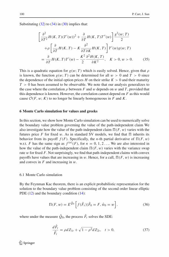
∂K 2 , K > 0, w > 0. (35)
This is a quadratic equation for g(w; T ) which is easily solved. Hence, given that ρ
is known, the function g(w; T ) can be determined for all w > 0 and T > 0 sincethe dependence of the initial option prices H on their strike K > 0 and their maturityT > 0 has been assumed to be observable. We note that our analysis generalizes tothe case where the correlation ρ between F and w depends on w and T , provided thatthis dependence is known. However, the correlation cannot depend on F as this wouldcause O(F, w; K ) to no longer be linearly homogeneous in F and K .
6 Monte Carlo simulation for values and greeks
In this section, we show how Monte Carlo simulation can be used to numerically solvethe boundary value problem governing the value of the path-independent claim Wealso investigate how the value of the path-independent claim �(F, w) varies with thefutures price F for fixed w. As in standard SV models, we find that � inherits itsbehavior from its payoff f (F). Specifically, the n-th partial derivative of �(F, w)
w.r.t. F has the same sign as f (n)(F), for n = 0, 1, 2 . . .. We are also interested inhow the value of the path-independent claim �(F, w) varies with the variance swaprate w for fixed F . Not surprisingly, we find that path-independent claims with convexpayoffs have values that are increasing in w. Hence, for a call, �(F, w) is increasingand convex in F and increasing in w.
6.1 Monte Carlo simulation
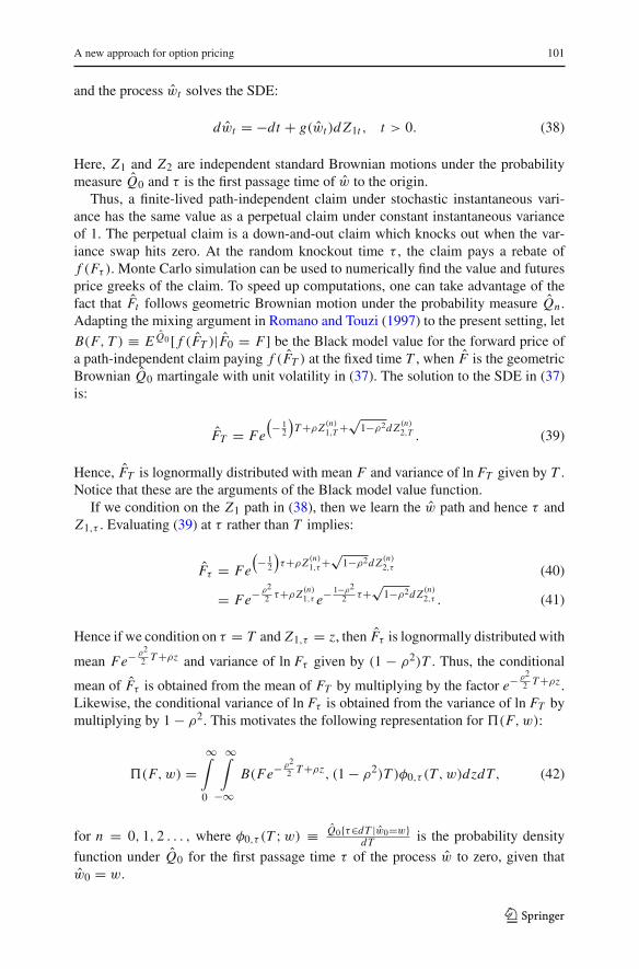
By the Feynman Kac theorem, there is an explicit probabilistic representation for thesolution to the boundary value problem consisting of the second order linear ellipticPDE (12) and the boundary condition (14):
�(F, w) = E Q0[
f (Fτ )|F0 = F, w0 = w]. (36)
where under the measure Q0, the process Ft solves the SDE:
d Ft
Ft= ρd Z1t +
√1 − ρ2d Z2t , t > 0, (37)
123
A new approach for option pricing 101
and the process wt solves the SDE:
dwt = −dt + g(wt )d Z1t , t > 0. (38)
Here, Z1 and Z2 are independent standard Brownian motions under the probabilitymeasure Q0 and τ is the first passage time of w to the origin.
Thus, a finite-lived path-independent claim under stochastic instantaneous vari-ance has the same value as a perpetual claim under constant instantaneous varianceof 1. The perpetual claim is a down-and-out claim which knocks out when the var-iance swap hits zero. At the random knockout time τ , the claim pays a rebate off (Fτ ). Monte Carlo simulation can be used to numerically find the value and futuresprice greeks of the claim. To speed up computations, one can take advantage of thefact that Ft follows geometric Brownian motion under the probability measure Qn .Adapting the mixing argument in Romano and Touzi (1997) to the present setting, let
B(F, T ) ≡ E Q0 [ f (FT )|F0 = F] be the Black model value for the forward price ofa path-independent claim paying f (FT ) at the fixed time T , when F is the geometricBrownian Q0 martingale with unit volatility in (37). The solution to the SDE in (37)is:
FT = Fe
(− 1
2
)T +ρZ (n)
1,T +√
1−ρ2d Z (n)2,T . (39)
Hence, FT is lognormally distributed with mean F and variance of ln FT given by T .Notice that these are the arguments of the Black model value function.
If we condition on the Z1 path in (38), then we learn the w path and hence τ andZ1,τ . Evaluating (39) at τ rather than T implies:
Fτ = Fe
(− 1
2
)τ+ρZ (n)
1,τ +√
1−ρ2d Z (n)2,τ (40)
= Fe− ρ2
2 τ+ρZ (n)1,τ e− 1−ρ2
2 τ+√
1−ρ2d Z (n)2,τ . (41)
Hence if we condition on τ = T and Z1,τ = z, then Fτ is lognormally distributed with
mean Fe− ρ2
2 T +ρz and variance of ln Fτ given by (1 − ρ2)T . Thus, the conditional
mean of Fτ is obtained from the mean of FT by multiplying by the factor e− ρ2
2 T +ρz .Likewise, the conditional variance of ln Fτ is obtained from the variance of ln FT bymultiplying by 1 − ρ2. This motivates the following representation for �(F, w):
�(F, w) =∞∫
0
∞∫
−∞B(Fe− ρ2
2 T +ρz, (1 − ρ2)T )φ0,τ (T, w)dzdT, (42)
for n = 0, 1, 2 . . . , where φ0,τ (T ;w) ≡ Q0{τ∈dT |w0=w}dT is the probability density
function under Q0 for the first passage time τ of the process w to zero, given thatw0 = w.
123
102 P. Carr, J. Sun
For many path-independent claims such as calls and puts, the Black model value in(42) is known in closed form. For such claims, one need only simulate the Q0 dynam-ics of w in (38). For each simulated w path terminating at wτ = 0, one just needsτ and Z1,τ to evaluate this closed form expression. The claim value is approximatedby averaging over paths. Since the barrier at zero is monitored continuously, a naivediscrete time Monte Carlo will tend to overvalue τ , producing upward bias in convexclaims. To remedy this, one can use Brownian bridges as discussed in Beaglehole et al.(1997), El Babsiri and Noel (1998), and in Andersen and Brotherton-Ratcliffe (1996).Alternatively, one can use large deviations as discussed in Baldi et al. (1999).
6.2 Partial derivatives
Since the process w in (38) is a univariate diffusion, a coupling argument impliesthat a rise in its initial value w weakly increases the first passage time to the ori-gin. If the payoff function f is convex, then since F is a Q0 martingale, the process{ f (Ft ), t > 0} is a Q0 submartingale. It follows that a rise in w causes � to increase.Hence, when f is convex, then the hedge ratio ∂�
∂w(F, w) is positive.
Similarly, one can use a coupling argument to show that the hedge ratio ∂�∂ F (F, w)
is nonnegative when f is increasing in F . More generally, the following theorem isproved in Appendix 1:
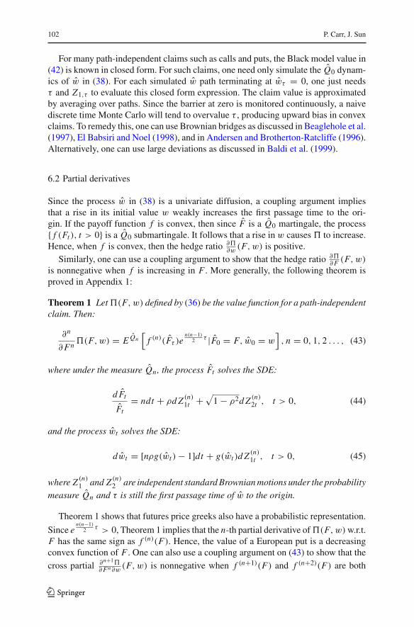
Theorem 1 Let �(F, w) defined by (36) be the value function for a path-independentclaim. Then:
∂n
∂ Fn�(F, w) = E Qn
[f (n)(Fτ )e
n(n−1)2 τ |F0 = F, w0 = w
], n = 0, 1, 2 . . . , (43)
where under the measure Qn, the process Ft solves the SDE:
d Ft
Ft= ndt + ρd Z (n)
1t +√
1 − ρ2d Z (n)2t , t > 0, (44)
and the process wt solves the SDE:
dwt = [nρg(wt ) − 1]dt + g(wt )d Z (n)1t , t > 0, (45)
where Z (n)1 and Z (n)
2 are independent standard Brownian motions under the probability
measure Qn and τ is still the first passage time of w to the origin.
Theorem 1 shows that futures price greeks also have a probabilistic representation.
Since en(n−1)
2 τ > 0, Theorem 1 implies that the n-th partial derivative of �(F, w) w.r.t.F has the same sign as f (n)(F). Hence, the value of a European put is a decreasingconvex function of F . One can also use a coupling argument on (43) to show that thecross partial ∂n+1�
∂ Fn∂w(F, w) is nonnegative when f (n+1)(F) and f (n+2)(F) are both
123
A new approach for option pricing 103
increasing in F . In particular, for n = 1, the vanna ∂2�∂ F∂w
(F, w) is nonnegative whenf (2)(F) and f (3)(F) are both increasing in F .
We can adapt the above mixing argument to also value futures price Greeks usingsimulation. As a special case of Theorem 1 with w = T and g(w) = 0:
∂n
∂ FnB(F, T ) = E Qn
[f (n)(FT )e
n(n−1)2 T |F0 = F
]
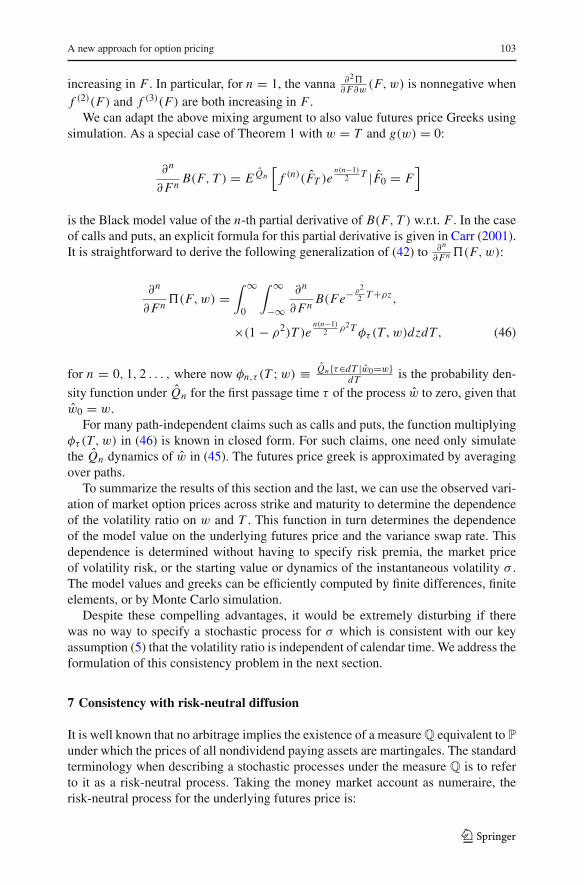
is the Black model value of the n-th partial derivative of B(F, T ) w.r.t. F . In the caseof calls and puts, an explicit formula for this partial derivative is given in Carr (2001).It is straightforward to derive the following generalization of (42) to ∂n
∂ Fn �(F, w):
∂n
∂ Fn�(F, w) =
∫ ∞
0
∫ ∞
−∞∂n
∂ FnB(Fe− ρ2
2 T +ρz,
×(1 − ρ2)T )en(n−1)
2 ρ2T φτ (T, w)dzdT, (46)
for n = 0, 1, 2 . . . , where now φn,τ (T ;w) ≡ Qn{τ∈dT |w0=w}dT is the probability den-
sity function under Qn for the first passage time τ of the process w to zero, given thatw0 = w.
For many path-independent claims such as calls and puts, the function multiplyingφτ (T, w) in (46) is known in closed form. For such claims, one need only simulatethe Qn dynamics of w in (45). The futures price greek is approximated by averagingover paths.
To summarize the results of this section and the last, we can use the observed vari-ation of market option prices across strike and maturity to determine the dependenceof the volatility ratio on w and T . This function in turn determines the dependenceof the model value on the underlying futures price and the variance swap rate. Thisdependence is determined without having to specify risk premia, the market priceof volatility risk, or the starting value or dynamics of the instantaneous volatility σ .The model values and greeks can be efficiently computed by finite differences, finiteelements, or by Monte Carlo simulation.
Despite these compelling advantages, it would be extremely disturbing if therewas no way to specify a stochastic process for σ which is consistent with our keyassumption (5) that the volatility ratio is independent of calendar time. We address theformulation of this consistency problem in the next section.
7 Consistency with risk-neutral diffusion
It is well known that no arbitrage implies the existence of a measure Q equivalent to P
under which the prices of all nondividend paying assets are martingales. The standardterminology when describing a stochastic processes under the measure Q is to referto it as a risk-neutral process. Taking the money market account as numeraire, therisk-neutral process for the underlying futures price is:
123
104 P. Carr, J. Sun
d Ft = √vt Ft d Bt , t ∈ [0, T ], (47)
where B is standard Brownian motion under Q. The risk-neutral drift of the futuresprice is zero, since futures contracts are costless. The process v in (47) is commonlyreferred to as the instantaneous variance. Under Q, the variance swap rate is the risk-neutral expected value of the remaining integral of v:
wt = EQ
[∫ T
tvudu
∣∣∣∣vt = v
], v ≥ 0, t ∈ [0, T ]. (48)
Under our SVRH, the risk-neutral process for w is given by:
dwt = −vt dt + g(wt )√
vt dWt , t ∈ [0, T ], (49)
where W is standard Brownian motion under Q. The risk-neutral drift of −vt dt in(55) reflects the fact that a long position in a variance swap results in a cash inflow ofvt dt at each instant of time. By Girsanov’s theorem, the two Brownian motions havethe same correlation under Q as they have under P:
d Bt dWt = ρdt. (50)
Suppose that in addition to (47) and (49), the risk-neutral dynamics of the instan-taneous variance rate are assumed to be given by:
dvt = a(t, vt )dt + b(t, vt )√
vt dWt , t ∈ [0, T ]. (51)
Notice that the Brownian motion W driving v is the same as the one driving w. Sincethe coefficients a and b in (51) are assumed to be independent of T , we refer to (51)as the maturity independent diffusion hypothesis (MIDH).
As we argue later, there is no economic justification for the MIDH. We believe thatthe only reason why the option pricing literature has adopted the MIDH is its inherenttractability and the lack of any plausible alternatives. Nonetheless, a great deal ofempirical work has been done testing the consistency of this class of models with thedata. Hence, it is of some interest to discern whether or not there is at least some sub-class of our stationary models for the w dynamics which is consistent with the MIDH(51). In the remainder of this section, we find a condition which the risk-neutral driftand diffusion coefficients of v must satisfy in order to meet both the MIDH and ourSVRH. In the next section, we find the only drift and diffusion functions for v whichmeet this condition.
Since we have Markovian dynamics for the instantaneous variance rate v, thereexists a C2,1 function w(v, t) : R
+ × [0, T ] �→ R+ such that the variance swap rate
wt is given by:
wt = w(t, vt ), t ∈ [0, T ]. (52)
123
A new approach for option pricing 105
By standard arbitrage arguments, this function w(t, v) solves the following secondorder linear parabolic PDE:
b2(t, v)v
2
∂2w
∂v2 (t, v) + a(t, v)∂w
∂v(t, v) + ∂w
∂t(t, v) = −v, (53)
on the domain t ∈ [0, T ], v ≥ 0. The function w is also subject to the terminalcondition:
w(T, v) = 0, v ≥ 0. (54)
The solution to the Cauchy problem consisting of (53) and (54) is unique.Applying Itô’s formula to (52) implies that the risk-neutral dynamics of the variance
swap rate w are given by:
dwt = −vt dt + ∂w
∂v(t, vt )b(t, vt )
√vt dWt , t ∈ [0, T ]. (55)
Since the form of the volatility function is invariant to the measure change, our objec-tive is to restrict the risk-neutral v dynamics so that the risk-neutral dynamics of w
obey:
dwt = −vt dt + g(wt )√
vt dWt , t ∈ [0, T ], (56)
where the function g(w) is independent of t and v. Comparing the diffusion coeffi-cients in (55) and (56), the question is whether one can specify the functions a(t, v)
and b(t, v) governing the risk-neutral dynamics of v in (51) so that:
∂w
∂v(t, v)b(t, v) = g(w(t, v)), t ∈ [0, T ], v ≥ 0, (57)
where w(t, v) solves (53) and (54) and g(w) is independent of t and v.Even if there exist solutions to (57), then a further open question is whether the
chosen g function gives sensible properties to w. For example, since v is a nonnegativeprocess, (48) implies that g(w) must be chosen so that w is also a nonnegative process:
wt ≥ 0, t ∈ [0, T ]. (58)
Furthermore, right at maturity, the variance swap rate is related to the instantaneousvariance rate by the following consistency condition:
limt↑T
wt
T − t= vT . (59)
Finally, since vT is finite, (59) implies the following terminal condition:
wT = 0. (60)
123
106 P. Carr, J. Sun
Since the nonnegativity condition (58), the consistency condition (59), and the terminalcondition (60) all refer to T , we will refer to them jointly as the T -conditions.
Since the coefficients of the w process in (56) are independent of t and the coeffi-cients of the v process in (51) are independent of T , it is not at all obvious whether thethree T -conditions can be achieved. Fortunately, the next section shows that the setof models satisfying both the SVRH and the MIDH is not empty. However, imposingthe SVRH on the class of maturity independent diffusion processes for v reduces therisk-neutral process for v to a diffusion with quadratic drift of the form p(t)vt + qv2
t
and with normal volatility proportional to v3/2t . Conversely, imposing the MIDH on
the class of time homogeneous continuous processes for w imposes a very specificstructure on the function g(w; T ) governing its normal volatility. Hence, the next sec-tion shows that only very specific risk-neutral processes for v and w are consistentwith the joint hypotheses of SVRH and MIDH.
8 The general solution to the consistency problem
This section shows that there exists a (maturity independent) risk-neutral diffusionprocess for v which is consistent with our SVRH. Fortunately, this process is bothempirically supported and tractable. The tractability arises from the fact that the jointFourier Laplace transform of returns and their quadratic variation can be derived inclosed form. We present this transform along with valuation formulas for the vari-ance swap rate and its volatility. The next section presents simpler formulas for thesequantities that arise in a subcase of the process presented in this section.
To emphasize which quantities are maturity dependent, the notation in this sec-tion will indicate maturity dependence whenever it is present. The following theoremshows that the SVRH and the MIDH completely determine the form of the risk-neutralprocess for v:
Theorem 2 The SVRH (5) and the MIDH (51) jointly imply that the risk-neutral pro-cess for the instantaneous variance is given by:
dvt = [p(t)vt + qv2t ]dt + εv
3/2t dWt , t ∈ [0, T ], (61)
where p is an arbitrary function of time and ε > 0 and q < ε2
2 are arbitrary constants.Furthermore, in the risk-neutral process for w:
dwt (T ) = −vt dt + g(wt (T ); T )√
vt dWt , t ∈ [0, T ], (62)
we must have g(0; T ) = 0 and gw(0; T ) = ε.
The proof of the above theorem is in Appendix 2. The content of Theorem 2 is thatonly a small set of risk-neutral processes for v are consistent with both our SVRH andthe MIDH. Theorem 4 of this section will also show that the function g governing thevolatility of w is much more restricted than as indicated in Theorem 2.
However, we caution that the small set of allowed processes for v and w is justas much due to the MIDH as our SVRH. The usual mechanism by which a maturity
123
A new approach for option pricing 107
independent risk-neutral diffusion process for v is derived is to assume a diffusionprocess for v under P and to assume that the market price of variance risk is a functionof just time t and the instantaneous variance v. To our knowledge, there is no economicjustification for either assumption. Rather, these assumptions are made solely for thepurpose of gaining the tractability associated with the risk-neutral v process being adiffusion. While tractability is a worthy objective, our approach of directly modellingthe variance swap rate dynamics already provides a tractable option pricing model.As a result, this justification for MIDH is absent in our setting. Consequently, anyunwelcome restrictions which the MIDH introduces to our setting can be banished bysimply rejecting it. We furthermore note that the maturity independence of the risk-neutral v process is only a consequence of the standard assumption that the moneymarket account serves as the numeraire. If the numeraire were instead some asset witha strictly positive payoff at T , then the drift and diffusion coefficients of v can dependon T . Hence, there is no need to have either maturity independence or a diffusionspecification for the risk-neutral process for the instantaneous variance.
Fortunately, the existing empirical literature examining the structure of the risk-neu-tral process for instantaneous variance is quite supportive of the one kind of processconsistent with both hypotheses. In particular, there is strong evidence in favor ofspecifying the diffusion coefficient of v as proportional to v
3/2t . There is also mildly
supportive evidence that the risk-neutral drift of v has the form p(t)vt +qv2t . The the-
oretical advantages of our SVRH models suggest that further empirical investigationalong these lines is warranted. However, should further testing reject the consistencyof the quadratic drift 3/2 process with the data, our view is that the theoretically andnumerically inferior MIDH should be jettisoned. Of course, we would advocate dis-posing of SVRH despite its advantages if direct empirical evidence were mountedagainst it.
Recall that the risk-neutral process for the underlying futures price is:
d Ft = √vt Ft d Bt , t ∈ [0, T ]. (63)
Theorem 2 implies that the v process in (63) satisfies the MIDH and our SVRH if andonly if:
dvt = [p(t)vt + qv2t ]dt + εv
3/2t dWt , t ∈ [0, T ], (64)
where p(t) is an arbitrary function of time, q < ε2
2 and ε > 0, and where:
d Bt dWt = ρdt. (65)
The reason for the upper bound on q becomes clear if we examine the process followedby:
Rt ≡ 1
vt, t ∈ [0, T ]. (66)
123
108 P. Carr, J. Sun
Employing Itô’s formula:
d Rt =[ε2 − q − p(t)Rt
]dt − ε
√Rt dWt , t ∈ [0, T ]. (67)
Thus, the reciprocal of V is just a special case of the affine drift square root process. Itis well known that this process avoids zero if ε2 −q > ε2
2 or equivalently q < ε2
2 . If qviolates this upper bound, then the v process can explode. As a result, we henceforthassume that q < ε2
2 . In fact, if q < 0, then by defining p(t) = κθ(t) and q = −κ forκ > 0, then (64) can be re-written as:
dvt = κvt [θ(t) − vt ]dt + εv3/2t dWt , t ∈ [0, T ]. (68)
Hence the risk-neutral process for v becomes mean-reverting, where the speed ofmean-reversion is proportional to v.
As (64) is actually more general than (68), we now further analyze the risk-neutral v process given in (64). With q respecting its upper bound, the results onthe reciprocal of v imply that the F and v processes respectively given by (63) and(61) never explode. Furthermore, for F0 > 0 and v0 > 0, the two processes are alwayspositive. If F0 = 0 or v0 = 0, then the corresponding process is trapped at the origin.As we assume that F0 > 0 and v0 > 0, this feature is of no economic consequence, butit does have the virtue of providing simple boundary conditions when employing finitedifferences. Although the v process is well-behaved under Q, Lewis (2000) shows thatoption pricing also requires that the v process have zero explosion probability underthe measure induced by taking the underlying asset as the numeraire. Feller’s explo-sion test implies that there is zero explosion probability under this measure if and onlyif ρ < 1
2ε. We henceforth impose this constraint which is automatically met if ρ ≤ 0
since ε > 0.The probability density function of RT is given in closed form in Cox et al. (1985),
when (67) is assumed to be time-homogeneous. It follows from (66) that the proba-bility density function for vT is also known by the change of variable formula, undertime-homogeneity. Other properties of the time-homogeneous version of the quadraticdrift 3/2 process are discussed in Ahn and Gao (1999), Andreasen (2001), Cox et al.(1980, 1985), Heston (1997), Lewis (2000), and Spencer (2003).
In particular, Heston (1997) points out that (64) is actually a generalization ofthe well-known CEV process, first proposed in Cox (1975). To see this, write therisk-neutral futures price process as:
d Ft
Ft= ηF
γ2
t d Bt , t ∈ [0, T ]. (69)
To ensure that F is a martingale rather than a strict local martingale, we require thatγ ∈ [0, 2]. Now let Vt ≡ V (Ft ) be the instantaneous variance rate, where from (69)the function V is defined by V (F) ≡ η2 Fγ for F > 0. Using Itô’s formula:
dVt = γ
2(γ − 1)V 2
t dt + γ V32
t d Bt , t ∈ [0, T ]. (70)
123
A new approach for option pricing 109
Hence, the CEV process can be obtained from (63) and (64) by setting p(t) = 0, q =γ2 (γ − 1), ε = γ , and ρ = 1.
By Girsanov’s theorem, the volatility of the instantaneous variance must have thesame form under P as it has under Q. Hence, Theorem 2 implies that the joint hypoth-eses of SVRH and MIDH force the normal volatility of v to be proportional to v
3/2t
under both P and Q. While this specification may seem unnatural, we note that if welet σt ≡ √
vt be the volatility, then Itô’s formula implies that the martingale part ofdσtσt
is ε2σt dWt . In words, the volatility of volatility is proportional to volatility. Hence,
the 3/2 specification is natural when posed in terms of the usual lognormal volatility.Although the 3/2 specification was derived purely from theoretical considerations,
it has received a surprisingly large amount of empirical support for both the statisticalprocess and the risk-neutral process. We first summarize the literature on the statisticalprocess. Using affine drift and a CEV specification for the volatility of instantaneousvariance, Ishida and Engle (2002) estimate the CEV power to be 1.71 for S&P500daily returns measured over a 30-year period. Javaheri (2004) also estimates this pro-cess on the time series of S&P500 daily returns, but with the CEV power constrainedto either be 0.5, 1.0, or 1.5. He concludes that for most of his filters, a power of 1.5outperforms the other two possible choices. Chacko and Viceira (1999) use SpectralGMM estimation on the same affine drift CEV process as in Ishida and Engle. Usingthe CRSP value weighted portfolio, they estimate the CEV power at 1.10 using weeklydata over a 35-year period and at 1.65 using monthly data over a 71-year period.
Two studies examine both the statistical process and the risk-neutral process.Poteshman (1998) examines S&P500 index option prices over a 7-year period andfinds that both the statistical and the risk-neutral drift of the instantaneous variance arenot affine. He also finds that the volatility of the instantaneous variance is an increasingconvex function of the instantaneous variance. Jones (2003) examines daily S&P100returns and implied volatilities over a 14-year period. Using this data, he first estimatesthe statistical version of the affine drift CEV process for the instantaneous variance.Using his time series of S&P100 daily returns, he finds the CEV power to be 1.33.Comparing the fit of this CEV model with the square root model on the option pricedata, he finds much better option pricing under the CEV model for 3- and 6- monthoptions. For shorter maturity options, all of his (purely continuous) models fail andso he concludes that jumps may be needed. Using the same data as in Jones (2003),Bakshi et al. (2004) look at a time series of S&P100 implied volatilities as capturedby V I X2. They estimate several models including an SDE of the form
dvt =(
α0 + α1vt + α2v2t + α3
vt
)dt + β2v
β3t dWt , t ∈ [0, T ]. (71)
They find that α2 and α3 are highly significant. They find that a linear drift model isrejected in favor of a nonlinear drift model. They find that the CEV power parameteris highly significant and estimate it at 1.27. They conduct a one sided t test on the nullhypotheseis that β3 ≤ 1 and reject this null. They conclude that β3 > 1 is needed tomatch the time series properties of the VIX index with CEV models.
We conclude that there is substantial evidence supporting a 3/2 power specifica-tion for the normal volatility of v. The evidence supporting the deterministically time
123
110 P. Carr, J. Sun
varying quadratic drift in Theorem 2 is weaker, but not inconsistent. The theoreticaland numerical advantages of the quadratic drift 3/2 process promulgated in Theorem2 suggests that further empirical work on this process is warranted.
Besides enjoying empirical support, the quadratic drift 3/2 process is also extremelytractable. Let Xt ≡ ln(Ft/F0) be the return process and let 〈X〉t ≡ ∫ t
0 vsds denoteits quadratic variation. Let EQ[eiu XT −s〈X〉T ] be the joint Fourier Laplace transform ofXT and 〈X〉T . Let EQ[eiu XT −s(〈X〉T −〈X〉t ]|Xt = x, vt = v] be the joint conditionalFourier Laplace transform of XT and 〈X〉T −〈X〉t . We now show that there is a closedform formula for the latter expression.
Theorem 3 Suppose that the risk-neutral process for the instantaneous variance isgiven by:
dvt = [p(t)vt + qv2t ]dt + εv
3/2t dWt , t ∈ [0, T ], (72)
where q < ε2
2 . Then the joint conditional Fourier Laplace transform of XT and〈X〉T − 〈X〉t is given by:
EQ[eiu XT −s(〈X〉T −〈X〉t
]|Xt = x, vt = v] = eiux �(γ − α)
�(γ )
(2
ε2 y(t, v)
)α
×M
(α; γ ; −2
ε2 y(t, v)
), (73)
where:
y(t, v) ≡∫ T
te∫ t ′
t p(u)dudt ′ × v, (74)
the confluent hypergeometric function M is defined as:
M(α; γ ; z) ≡∞∑
n=0
(α)n
(γ )n
zn
n! ,
α ≡ −(
1
2− q
ε2
)+
√(1
2− q
ε2
)2
+ 2λ
ε2 ,
γ ≡ 2
[α + 1 − q
ε2
], (75)
and where:
q ≡ q + ρεiu λ ≡ s + iu
2+ u2
2.
123
A new approach for option pricing 111
The proof of Theorem 3 is in Appendix 3. The result in Theorem 3 makes it straight-forward to numerically value many derivative securities written on XT and/or 〈X〉T .In particular, the prices of European options on FT can be quickly obtained via (fast)Fourier inversion. Assuming time homogeneity, Heston (1997) and Lewis (2000) haveindependently derived the conditional characteristic function of XT . Our result extendsthese previously derived results in two ways. First, we have the joint transform whichallows us to value both options on price and options on realized variance, or evenoptions on both. Second, we have obtained this joint Fourier Laplace transform despitethe fact that the risk-neutral drift of v contains an arbitrary function of time. This fea-ture allows one to calibrate the quadratic drift to an arbitrarily given term structure ofsay ATM implied volatilities or variance swap rates. It also allows one to generalizethe model by randomizing the level towards which the v process reverts. If the risk-neutral process for this level evolves independently of F and v then the risk-neutraldensity for a functional of this process can be chosen so as to gain consistency withan implied volatility skew.
We now turn to the implication of our SVRH and the MIDH for the form ofw(v, t; T ) and the form of the function g(w; T ) determining its normal volatility.The following theorem shows that both functions are determined in closed form.
Theorem 4 Suppose that the risk-neutral process for the instantaneous variance isgiven by:
dvt = [p(t)vt + qv2t ]dt + εv
3/2t dWt , t ∈ [0, T ], (76)
where q < ε2
2 . Then the variance swap rate valuation function w(t, v; T ) ≡ EQ[∫ Tt vudu
∣∣∣∣vt = v
]is given by:
w(t, v; T ) = h
(v ×
∫ T
te∫ t ′
t p(u)dudt ′)
, t ∈ [0, T ], v ≥ 0, T > 0, (77)
where:
h(y) =∫ y
0e− 2
ε2z z− 2q
ε2
∫ ∞
z
2
ε2 e2
ε2u u2qε2 −2
dudz. (78)
The risk-neutral process for the variance swap rate is given by:
dwt (T ) = −vt dt + g(wt (T ))√
vt dWt , t ∈ [0, T ], (79)
where:
g(w) = ε∂
∂yh(h−1(w)))h−1(w), w > 0, (80)
where h−1(w) is the inverse in w of h(w).
123
112 P. Carr, J. Sun
The proof of Theorem 4 is in Appendix 4. This proof makes it clear that the 3T -conditions (58) to (60) are all met. By the equivalence of Q and P, these conditionsalso hold for the statistical process for w provided that it retains the same form.
Clearly, the general forms for w and g are complicated. To address this deficiency,we offer three solutions. First, Appendix 4 shows that h solves the simple linear ODE:
ε2 y2
2
∂2
∂y2 h(y) + (qy − 1)∂
∂yh(y) + 1 = 0, y > 0, (81)
subject to h(0) = 0 and limy↓0
∂∂y h(y) = 1. Furthermore, Appendix 4 also shows that
g(w) solves the following nonlinear ODE:
g2(w)
2g′′(w) + ε
2g(w)g′(w) +
(q − 1 − ε2
2
)g(w) + ε = 0, (82)
subject to g(0) = 0 and g′(0) = ε. In applied work, it may be easier to numericallyevaluate these boundary value problems for h and g rather than their solution given inTheorem 4.
A second approach for dealing with the complexity of w and its volatility is toswitch attention from w to a related process. Suppose we define a stochastic process{yt ; t ∈ [0, T ]} by:
yt ≡ EQt
∫ T
te−q
∫ t ′t vuduvt ′dt ′, t ∈ [0, T ]. (83)
Note that the parameter q in (83) is the same as the one used in Theorem 2 and hence werequire q < ε2/2. A financial interpretation of y is that it represents the value at time tof the floating part of a dynamic trading strategy in variance swaps. For each t ′ ∈ [t, T ],this strategy holds e−q
∫ t ′t vudu variance swaps. Since the v process is Markovian in
itself and time, it follows that there exists a C1,2 function y(t, v) : [0, T ]×R+ �→ R
+such that:
yt = y(t, vt ), t ∈ [0, T ]. (84)
By the Feynman Kac Theorem, the function y(t, v) solves the following PDE:
ε2v3
2
∂2 y
∂v2 (t, v) +[
p(t)v + qv2] ∂y
∂v(t, v) + ∂y
∂t(t, v) = qvy(t, v) − v, (85)
on the domain t ∈ [0, T ], v ≥ 0. The function y is also subject to the terminalcondition:
y(T, v) = 0, v ≥ 0. (86)
The solution to the Cauchy problem consisting of (85) and (86) is unique.
123
A new approach for option pricing 113
Given that q and ε are both in the above Cauchy problem, it is remarkable thatgiven vt = v, the solution for the value of yt is always independent of both q and ε.Intuitively, the independence of y from q arises because the dynamic trading strategyin variance swaps offsets the dependence of w on q. The independence of y from ε
arises because y is just proportional to v:
yt =∫ T
te∫ t ′
t p(u)dudt ′ × vt , t ∈ [0, T ]. (87)
It is straightforward to verify that (87) solves (85) and (86). Applying Itô’s formula to(87), (76) implies that the risk-neutral dynamics of y are given by:
dyt = (qyt − 1)vt dt + εyt√
vt dWt , t ∈ [0, T ]. (88)
Hence, the level of y in (87) is independent of q and ε, but this level does dependon the function p. Conversely, the dynamics of y in (88) depends on q and ε, butthese dynamics are independent of the function p. Notice also that the y dynamicsin (88) are time homogeneous in both calendar time and business time defined by〈X〉t = ∫ t
0 vsds. Comparing (79) and (88), we see that although y has a slightly morecomplicated risk-neutral drift than w, it has much simpler volatility.
The definition (83) of y makes it clear that it is positive before T and vanishesright at T . Since the dynamics of y are independent of t and the dynamics of v areindependent of T , it is somewhat surprising that the process y is positive before T andvanishes right at T . The intuition for this result is best seen when p(t) = p. At first,this seems even more puzzling since v is then also a time homogeneous diffusion.However from (87):
yt = vte p(T −t) − 1
p. (89)
Hence, the ratio of the two time-homogeneous diffusion processes is just a functionof the time to maturity.
The process y has the same qualitative behavior as w in that they both proxy forboth time to maturity and the risk-neutral expectation of remaining volatility. Recallthat under SVRH, it is sufficient to use the pair (F, w) as state variables in place ofthe triple (F, v, t). Likewise, the time homogeneity of the y process makes it possibleto use use the pair (F, y) as state variables in place of this triple. Furthermore, themuch simpler form of the volatility of y suggests that the pair (F, y) should be usedin place of (F, w).
The definition (83) of y makes it clear that it reduces to w when q = 0. Thissuggests that the complexity of w vanishes if we simply assume that the risk-neutralprocess for v has no quadratic component. Compared to modelling the y process, thisthird approach for dealing with the complexity of w has the disadvantage of imposingstructure on the risk-neutral drift of v that may not be supported by the (options) data.However, it has the conceptual advantage of focussing our assumptions concerningprice dynamics on a static position in variance swaps, rather than a dynamic one.
123
114 P. Carr, J. Sun
As the traditional approach in the asset pricing literature has been to place structureon the price dynamics of a static position, the next section elaborates on this finalapproach for dealing with the complexity of w and its volatility.
9 Simple variance swap rate dynamics
This section shows that setting q = 0 in the risk-neutral drift of v leads to much simplervaluation formulas and dynamics for w. In particular, the value function w(v, t; T )
becomes proportional to v, while the function g(w; T ) governing w’s volatility be-comes proportional to w. Setting q = 0 in the risk-neutral drift of v does imply that itno longer mean reverts to a positive level. However, it should be remembered that thisproperty applies only to the risk-neutral process. We show that a standard specificationfor the market price of v risk results in a specification of the statistical v process whichis just the quadratic drift 3/2 process discussed in the last section. Hence, the tracta-bility of the risk-neutral process discussed in the last section extends to the statisticalprocess to be discussed in this one. The quadratic drift in the statistical v process canbe interpreted as providing mean-reversion to a positive level. The novelty comparedto standard affine models is that the speed of mean-reversion is proportional to thelevel of v. As already mentioned, the martingale component of this statistical processhas received much empirical support.
In this section, we assume that the dynamics of v under Q are given by:
dvt = p(t)vt dt + εv3/2t dWt , t ∈ [0, T ]. (90)
In other words, we have set q = 0 in the only v dynamics consistent with both ourSVRH and the MIDH. Setting q = 0 in the ODE (81) implies that it simplifies to:
ε2 y2
2
∂2
∂y2 h(y) − ∂
∂yh(y) + 1 = 0, y > 0, (91)
A simple solution which meets the boundary conditions h(0) = 0 and limy↓0
∂∂y h(y) = 1
is:
h(y) = y, y > 0. (92)
As a consequence, (77) implies that the variance swap rate is proportional to v:
w(t, v; T ) =∫ T
te∫ t ′
t p(u)dudt ′v, t ∈ [0, T ], v ≥ 0, T > 0. (93)
Recall from the last section that the probability density function of vT is known fromthe work of Cox et al. (1985), when the risk-neutral v process is time-homogeneous.It follows from (93) that the probability density function for wT is also known by thechange of variable formula, under time-homogeneity of the risk-neutral v process.
123
A new approach for option pricing 115
As (92) implies that ∂∂w
h(w) = 1 and h−1(w) = w, (80) implies that:
g(w) = εw, w ≥ 0, T > 0. (94)
Hence, the risk-neutral w dynamics simplify to:
dwt (T ) = −vt dt + εwt (T )√
vt dWt , t ∈ [0, T ]. (95)
Since ε also appears in the v dynamics, it must be independent of T . Hence, ourmodel (95) makes the strong empirical prediction that variance swap rates of differentmaturities have the same (lognormal) volatility. This feature is not shared by the moregeneral solution of the last section.
As for the statistical process for v, we know that the volatility is the same under P
and Q. In contrast, the drift under the statistical measure P is:
EP[dvt |vt , t] = [p(t)vt + λ(vt , t)]dt. (96)
Suppose that we specify the following quadratic form for the market price of v risk:
λ(v, t) = λ0(t) + λ1(t)v + λ2(t)v2, v ≥ 0, t ∈ [0, T ]. (97)
Then from (96) and (97), the statistical drift of v is
EP[dvt |vt , t] = {λ0(t) + κ(t)vt [θ(t) − vt ]}dt, (98)
where κ(t) ≡ −λ2(t) and θ(t) ≡ − p(t)+λ1(t)λ2(t)
. We assume that λ2(t) < 0 and λ1(t) >
−p(t) so that κ(t) > 0 and θ(t) > 0. Now recall that zero is a natural boundary forthe risk-neutral process for v in (61). Thus a process which starts at zero stays thereforever. However, if the statistical drift is given by (98), then a process which starts atzero moves away from zero unless:
λ0(t) = 0. (99)
Since P and Q must be equivalent probability measures, we set λ0(t) = 0 and hencethe statistical process for v simplifies to:
dvt = κ(t)vt [θ(t) − vt ]dt + εv3/2t dWt , t ∈ [0, T ]. (100)
Hence, at each t ∈ [0, T ], the process is mean-reverting towards θ(t) > 0 with a speedof mean-reversion κ(t)vt > 0. As a result, we refer to the process described in (100)as the mean-reverting 3/2 process.
Finally, we turn to the statistical dynamics for the variance swap rate w. From(97) and (99), the absolute drift compensation at time t for exposure to εv
3/2t dWt
123
116 P. Carr, J. Sun
is λ1(t)vt + λ2(t)v2t . Since the martingale component of dwt is just wt
vttimes the
martingale component of dvt it follows that:
πwt wt = wt
vt[λ1(t)vt + λ2(t)v
2t ], t ∈ [0, T ]. (101)
Simplifying implies that w′s relative risk premium is affine in v:
πwt = λ1(t) + λ2(t)vt , t ∈ [0, T ]. (102)
Restricting dynamics to the model specified in this section, (12) and (94) imply thatthe valuation function �(F, w) for a path-independent claim satisfies the followingsecond order linear elliptic PDE:
F2
2
∂2�
∂ F2 (F, w) + ρεwF∂2�
∂w∂ F(F, w) + ε2w2
2
∂2�
∂w2 (F, w) − ∂�
∂w(F, w) = 0,
(103)
on the domain F > 0, w > 0. We further require that �(F, w) satisfy the boundaryconditions:
�(F, 0) = f (F), F > 0, (104)
�(0, w) = f (0), w > 0, (105)
and satisfy growth conditions as F and w become infinite.Note that this valuation model is extremely parsimonious. The forward price of an
option can be numerically valued once one knows its strike price, the futures price ofthe underlying asset, the initial variance swap rate of the same maturity, and the twoparameters ρ and ε. The average level of the implied volatility smile of maturity T ispositively related to the observable variance swap rate wt . The average slope of thesmile is positively related to the correlation parameter ρ. The average curvature of thesmile is positively related to the volvol parameter ε.
One can use finite differences or finite elements to numerically solve the aboveboundary value problem. One can also use Monte Carlo simulation of just the vari-ance swap rate over an infinite horizon as discussed in Sect. 6. Alternatively, one canuse the Romano Touzi trick to just simulate v over a finite horizon using (61). Thechoice of whether to simulate w or v depends on how close w is to the origin.
Recall that the last section derived the joint Fourier Laplace transform of XT and〈X〉T under the quadratic drift 3/2 process for v. Of course, this formula can be appliedto our current setting of proportional risk-neutral drift simply by setting q = 0. Fur-thermore, we can substitute out v and t for w to instead relate this transform andits derived quantities to the more observable variance swap rate. When calibratingan option pricing model, it is useful if call values can be efficiently expressed as afunction of strike price. Since the characteristic function of ln FT is a known analyticfunction of ln F , w, and t , the results of Carr and Madan (1999) imply that the fastFourier transform (FFT) can be used to efficiently obtain call values as a function of
123
A new approach for option pricing 117
log strike. As shown in Chourdakis (2004), the fractional FFT can be used to speedup results even further.
10 Pricing and hedging volatility derivatives
10.1 Pricing and hedging derivatives on realized variance
Before variance swaps became active, swaps were traded over-the-counter on realizedvolatility. Since volatility is the square root of realized variance, a volatility swap isa derivative security on realized variance. Recently, options on realized variance andoptions on realized volatility also became available.
To value derivatives on realized variance, recall the assumptions made on the futuresprice F and the variance swap rate w under the statistical measure P:
d Ft
Ft= µt dt + √
vt d Bt , (106)
dwt = (πwt wt − vt )dt + g(wt )
√vt dWt , t ∈ [0, T ], (107)
where:
d Bt dWt = ρdt, t ∈ [0, T ]. (108)
It turns out that to value derivatives on realized variance, only the w dynamics arerelevant. Hence for the rest of the paper, we can let the futures price jump and we needno assumption on the nature of the correlation between the two Brownian motions Band W .
Let Xt ≡ ln(Ft/F0) be the log price relative and let 〈X〉t = ∫ t0 vsds be its qua-
dratic variation. We assume that the payoff on the volatility derivative is some knownfunction of just 〈X〉T . Let V(w, q) : R
+ × R+ �→ R be a C2,1 function and let
Vt ≡ V(wt , 〈X〉t ) be a continuous stochastic process. Itô’s formula implies that:
V(wT , 〈X〉T ) = V(w0, 0) +∫ T
0
∂
∂wV(wt , 〈X〉t )dwt +
∫ T
0
∂
∂qV(wt , 〈X〉t )d〈X〉t
+∫ T
0
g2(wt )
2
∂2V∂w2 (wt , 〈X〉t )vt dt. (109)
Suppose that we add and subtract∫ T
0∂
∂wV(Ft , wt )vt dt . Then V(wT , 〈X〉T ):
= V(w0, 0) +∫ T
0
∂
∂wV(wt , 〈X〉t )(dwt + vt dt) +
∫ T
0
[∂
∂qV(wt , 〈X〉t )
+g2(wt )
2
∂2
∂w2 V(wt , 〈X〉t ) − ∂
∂wV(wt , 〈X〉t )
]vt dt. (110)
123
118 P. Carr, J. Sun
Suppose that the function V(F, w) solves the following second order linear parabolicPDE:
∂V∂q
(w, q) + g2(w)
2
∂2V∂w2 (w, q) − ∂V
∂w(w, q) = 0, w > 0, q > 0. (111)
Further suppose that:
V(0, q) = f (q), q > 0. (112)
Since wT = 0, substitution of (111) and (112) in (110) implies:
f (〈X〉T ) = V(w0, 0) +∫ T
0
∂
∂wV(wt , 〈X〉t )(dwt + vt dt). (113)
Thus the payoff on the volatility derivative can be exactly replicated if one chargesV(w0, 0) initially and holds ∂
∂wV(wt , 〈X〉t ) variance swaps at each t ∈ [0, T ].
As in the last section, time is irrelevant because the realized volatility derivativematures at the same time as the variance swap. The boundary value problem (111)and (112) has the same computational complexity as the one arising under a standardstochastic volatility model. However, once again we do not need to know the dynamicsof the instantaneous variance or know the market price of volatility risk.
If finite differences are used to numerically determine the value function V(w, q)
on a grid, then one usually supplies 3 boundary conditions. To illustrate, supposewe wish to numerically determine the value of a put on realized variance. Then oneboundary condition is:
V(0, q) =(
K − q
T
)+, q > 0. (114)
As w gets large, it will take a lot of realized quadratic variation to bring it down tozero and hence:
limw↑∞ V(0, q) = 0, q > 0. (115)
Finally, since quadratic variation can only increase, the final boundary condition is:
V(w, K T ) = 0, w > 0. (116)
The PDE can be solved on the domain q ∈ [0, K T ], w > 0.When we specialize to the dynamics of the last section, the valuation PDE simplifies
to:
∂V∂q
(w, q) + ε2w2
2
∂2V∂w2 (w, q) − ∂V
∂w(w, q) = 0, w > 0, q > 0. (117)
123
A new approach for option pricing 119
If one wants a supporting SV model where the risk-neutral process for v is a diffusionwith maturity independent coefficients, then one should also assume a continuousfutures price process, constant correlation, and the quadratic drift 3/2 process (61) forinstantaneous variance.
It is also possible to write down the fundamental PDE operating for a European-style claim when the terminal payoff depends on both the spot price and the realizedvariance of returns. For example, the payoff could be the realized Sharpe ratio. In thiscase, we need to assume the continuous dynamics in (106) to (108). There are threeindependent variables F , w, and q in the PDE and it also has the same form as the PDEarising in a stochastic volatility model. Since we are not yet aware of any contractswith this complexity, we leave the details to the reader.
10.2 Pricing and hedging derivatives on the variance swap rate
The CBOE recently revamped the definition of its well known volatility index knownas the VIX. The new VIX is an average of two synthetic variance swap rates with theweights deterministically varying over time in such a way that the time to maturityis fixed at 30 days. Once a month, only one synthetic variance swap rate is used tocalculate the VIX and by design, this date is also the maturity date for VIX futures,which began trading in March 2004. It turns out that VIX futures at time t are valuedby determining the risk-neutral mean of
√wS , where S ∈ (t, T ) is the futures maturity
date. Hence, VIX futures is an example of a derivative security written on a varianceswap rate.
To value derivatives of this kind, let st be the value at time t ∈ [0, S] of the varianceswap rate for maturity S:
st = EQ
∫ S
tvudu, t ∈ [0, S]. (118)
Working under P, we assume that the dynamics of this variance swap rate are givenby:
dst = (π st st − vt )dt + h(st )
√vt d Bt , t ∈ [0, S], (119)
where B is a standard Brownian motion under P. Here, π s is a stochastic processrepresenting compensation for h(st ) differing from zero. Also, h(s) is a function ofjust s and is independent of t and v. We continue to assume that the statistical processfor w is given by (9), which we repeat here for convenience:
dwt = (πwt wt − vt )dt + g(wt )
√vt dWt , t ∈ [0, S], (120)
where g(w) is a function of just w and is independent of t and v. We assume that thecorrelation between the increments of the two variance swap rates is a function of thetwo rates:
d Bt dWt = ρ(st , wt )dt, t ∈ [0, S]. (121)
123
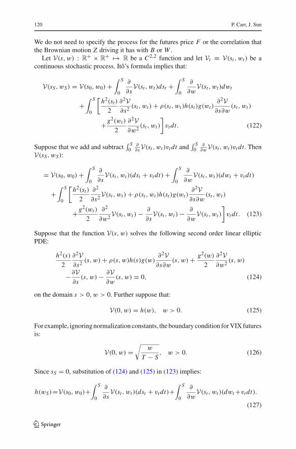
120 P. Carr, J. Sun
We do not need to specify the process for the futures price F or the correlation thatthe Brownian motion Z driving it has with B or W .
Let V(s, w) : R+ × R
+ �→ R be a C2,2 function and let Vt ≡ V(st , wt ) be acontinuous stochastic process. Itô’s formula implies that:
V(sS, wS) = V(s0, w0) +∫ S
0
∂
∂sV(st , wt )dst +
∫ S
0
∂
∂wV(st , wt )dwt
+∫ S
0
[h2(st )
2
∂2V∂s2 (st , wt ) + ρ(st , wt )h(st )g(wt )
∂2V∂s∂w
(st , wt )
+g2(wt )
2
∂2V∂w2 (st , wt )
]vt dt. (122)
Suppose that we add and subtract∫ S
0∂∂s V(st , wt )vt dt and
∫ S0
∂∂w
V(st , wt )vt dt . ThenV(sS, wS):
= V(s0, w0) +∫ S
0
∂
∂sV(st , wt )(dst + vt dt) +
∫ S
0
∂
∂wV(st , wt )(dwt + vt dt)
+∫ S
0
[h2(st )
2
∂2
∂s2 V(st , wt ) + ρ(st , wt )h(st )g(wt )∂2V∂s∂w
(st , wt )
+g2(wt )
2
∂2
∂w2 V(st , wt ) − ∂
∂sV(st , wt ) − ∂
∂wV(st , wt )
]vt dt. (123)
Suppose that the function V(s, w) solves the following second order linear ellipticPDE:
h2(s)
2
∂2V∂s2 (s, w) + ρ(s, w)h(s)g(w)
∂2V∂s∂w
(s, w) + g2(w)
2
∂2V∂w2 (s, w)
−∂V∂s
(s, w) − ∂V∂w
(s, w) = 0, (124)
on the domain s > 0, w > 0. Further suppose that:
V(0, w) = h(w), w > 0. (125)
For example, ignoring normalization constants, the boundary condition for VIX futuresis:
V(0, w) =√
w
T − S, w > 0. (126)
Since sS = 0, substitution of (124) and (125) in (123) implies:
h(wS)=V(s0, w0)+∫ S
0
∂
∂sV(st , wt )(dst + vt dt)+
∫ S
0
∂
∂wV(st , wt )(dwt +vt dt).
(127)
123
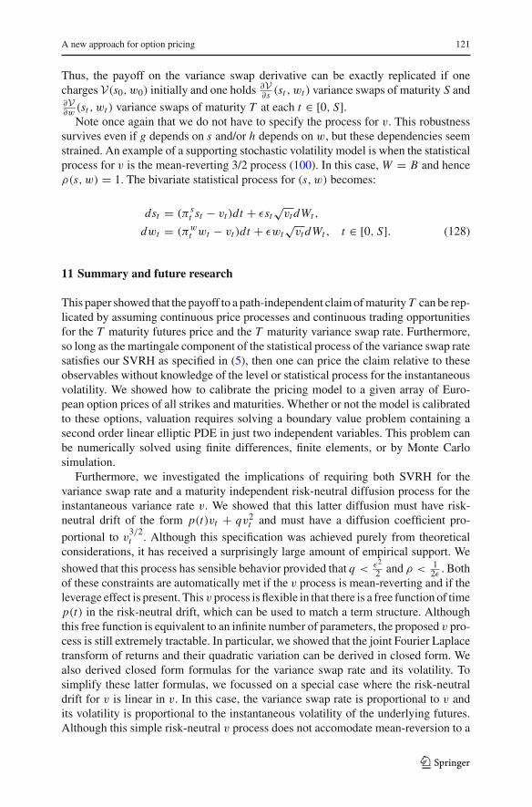
A new approach for option pricing 121
Thus, the payoff on the variance swap derivative can be exactly replicated if onecharges V(s0, w0) initially and one holds ∂V
∂s (st , wt ) variance swaps of maturity S and∂V∂w
(st , wt ) variance swaps of maturity T at each t ∈ [0, S].Note once again that we do not have to specify the process for v. This robustness
survives even if g depends on s and/or h depends on w, but these dependencies seemstrained. An example of a supporting stochastic volatility model is when the statisticalprocess for v is the mean-reverting 3/2 process (100). In this case, W = B and henceρ(s, w) = 1. The bivariate statistical process for (s, w) becomes:
dst = (π st st − vt )dt + εst
√vt dWt ,
dwt = (πwt wt − vt )dt + εwt
√vt dWt , t ∈ [0, S]. (128)
11 Summary and future research
This paper showed that the payoff to a path-independent claim of maturity T can be rep-licated by assuming continuous price processes and continuous trading opportunitiesfor the T maturity futures price and the T maturity variance swap rate. Furthermore,so long as the martingale component of the statistical process of the variance swap ratesatisfies our SVRH as specified in (5), then one can price the claim relative to theseobservables without knowledge of the level or statistical process for the instantaneousvolatility. We showed how to calibrate the pricing model to a given array of Euro-pean option prices of all strikes and maturities. Whether or not the model is calibratedto these options, valuation requires solving a boundary value problem containing asecond order linear elliptic PDE in just two independent variables. This problem canbe numerically solved using finite differences, finite elements, or by Monte Carlosimulation.
Furthermore, we investigated the implications of requiring both SVRH for thevariance swap rate and a maturity independent risk-neutral diffusion process for theinstantaneous variance rate v. We showed that this latter diffusion must have risk-neutral drift of the form p(t)vt + qv2
t and must have a diffusion coefficient pro-
portional to v3/2t . Although this specification was achieved purely from theoretical
considerations, it has received a surprisingly large amount of empirical support. Weshowed that this process has sensible behavior provided that q < ε2
2 and ρ < 12ε
. Bothof these constraints are automatically met if the v process is mean-reverting and if theleverage effect is present. This v process is flexible in that there is a free function of timep(t) in the risk-neutral drift, which can be used to match a term structure. Althoughthis free function is equivalent to an infinite number of parameters, the proposed v pro-cess is still extremely tractable. In particular, we showed that the joint Fourier Laplacetransform of returns and their quadratic variation can be derived in closed form. Wealso derived closed form formulas for the variance swap rate and its volatility. Tosimplify these latter formulas, we focussed on a special case where the risk-neutraldrift for v is linear in v. In this case, the variance swap rate is proportional to v andits volatility is proportional to the instantaneous volatility of the underlying futures.Although this simple risk-neutral v process does not accomodate mean-reversion to a
123
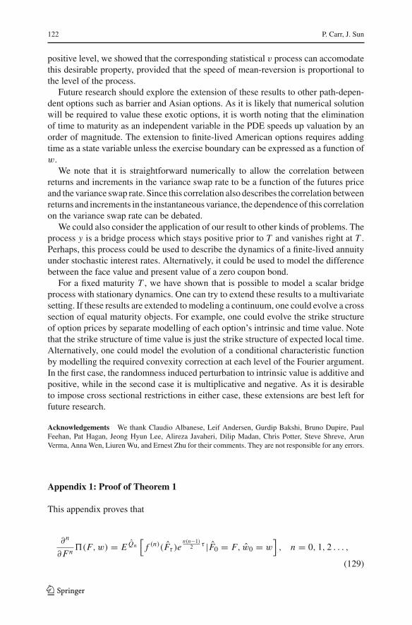
122 P. Carr, J. Sun
positive level, we showed that the corresponding statistical v process can accomodatethis desirable property, provided that the speed of mean-reversion is proportional tothe level of the process.
Future research should explore the extension of these results to other path-depen-dent options such as barrier and Asian options. As it is likely that numerical solutionwill be required to value these exotic options, it is worth noting that the eliminationof time to maturity as an independent variable in the PDE speeds up valuation by anorder of magnitude. The extension to finite-lived American options requires addingtime as a state variable unless the exercise boundary can be expressed as a function ofw.
We note that it is straightforward numerically to allow the correlation betweenreturns and increments in the variance swap rate to be a function of the futures priceand the variance swap rate. Since this correlation also describes the correlation betweenreturns and increments in the instantaneous variance, the dependence of this correlationon the variance swap rate can be debated.
We could also consider the application of our result to other kinds of problems. Theprocess y is a bridge process which stays positive prior to T and vanishes right at T .Perhaps, this process could be used to describe the dynamics of a finite-lived annuityunder stochastic interest rates. Alternatively, it could be used to model the differencebetween the face value and present value of a zero coupon bond.
For a fixed maturity T , we have shown that is possible to model a scalar bridgeprocess with stationary dynamics. One can try to extend these results to a multivariatesetting. If these results are extended to modeling a continuum, one could evolve a crosssection of equal maturity objects. For example, one could evolve the strike structureof option prices by separate modelling of each option’s intrinsic and time value. Notethat the strike structure of time value is just the strike structure of expected local time.Alternatively, one could model the evolution of a conditional characteristic functionby modelling the required convexity correction at each level of the Fourier argument.In the first case, the randomness induced perturbation to intrinsic value is additive andpositive, while in the second case it is multiplicative and negative. As it is desirableto impose cross sectional restrictions in either case, these extensions are best left forfuture research.
Acknowledgements We thank Claudio Albanese, Leif Andersen, Gurdip Bakshi, Bruno Dupire, PaulFeehan, Pat Hagan, Jeong Hyun Lee, Alireza Javaheri, Dilip Madan, Chris Potter, Steve Shreve, ArunVerma, Anna Wen, Liuren Wu, and Ernest Zhu for their comments. They are not responsible for any errors.
Appendix 1: Proof of Theorem 1
This appendix proves that
∂n
∂ Fn�(F, w) = E Qn
[f (n)(Fτ )e
n(n−1)2 τ |F0 = F, w0 = w
], n = 0, 1, 2 . . . ,
(129)
123
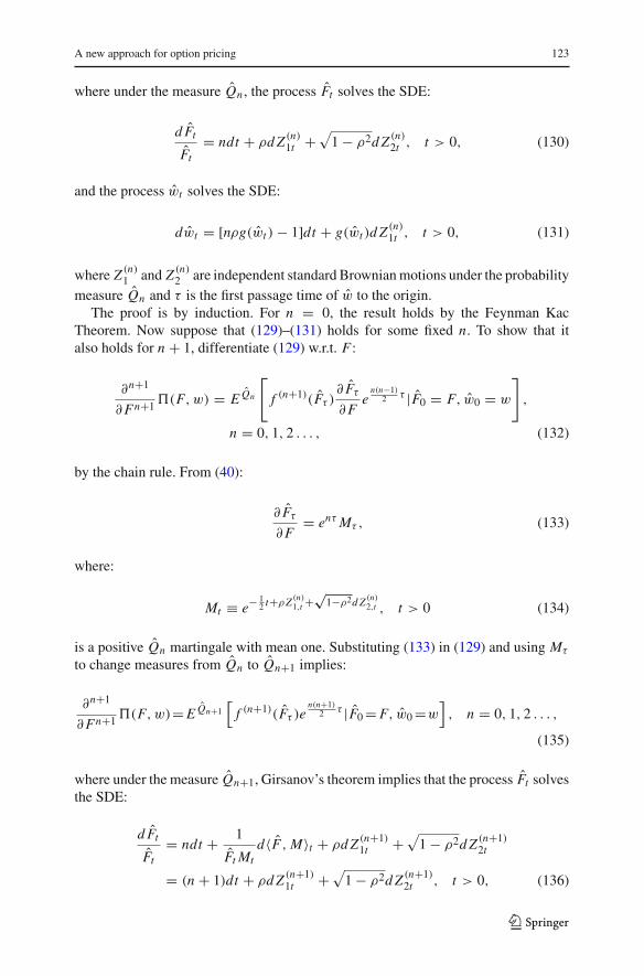
A new approach for option pricing 123
where under the measure Qn , the process Ft solves the SDE:
d Ft
Ft= ndt + ρd Z (n)
1t +√
1 − ρ2d Z (n)2t , t > 0, (130)
and the process wt solves the SDE:
dwt = [nρg(wt ) − 1]dt + g(wt )d Z (n)1t , t > 0, (131)
where Z (n)1 and Z (n)
2 are independent standard Brownian motions under the probabilitymeasure Qn and τ is the first passage time of w to the origin.
The proof is by induction. For n = 0, the result holds by the Feynman KacTheorem. Now suppose that (129)–(131) holds for some fixed n. To show that italso holds for n + 1, differentiate (129) w.r.t. F :
∂n+1
∂ Fn+1 �(F, w) = E Qn
[f (n+1)(Fτ )
∂ Fτ
∂ Fe
n(n−1)2 τ |F0 = F, w0 = w
],
n = 0, 1, 2 . . . , (132)
by the chain rule. From (40):
∂ Fτ
∂ F= enτ Mτ , (133)
where:
Mt ≡ e− 12 t+ρZ (n)
1,t +√
1−ρ2d Z (n)2,t , t > 0 (134)
is a positive Qn martingale with mean one. Substituting (133) in (129) and using Mτ
to change measures from Qn to Qn+1 implies:
∂n+1
∂ Fn+1 �(F, w)= E Qn+1[
f (n+1)(Fτ )en(n+1)
2 τ |F0 = F, w0 =w], n = 0, 1, 2 . . . ,
(135)
where under the measure Qn+1, Girsanov’s theorem implies that the process Ft solvesthe SDE:
d Ft
Ft= ndt + 1
Ft Mtd〈F, M〉t + ρd Z (n+1)
1t +√
1 − ρ2d Z (n+1)2t
= (n + 1)dt + ρd Z (n+1)1t +
√1 − ρ2d Z (n+1)
2t , t > 0, (136)
123
124 P. Carr, J. Sun
and the process wt solves the SDE:
dwt = [nρg(wt ) − 1]dt + 1
Mtd〈w, M〉t + g(wt )d Z (n+1)
1t
= [(n + 1)ρg(wt ) − 1]dt + g(wt )d Z (n+1)1t , t > 0, (137)
where Z (n+1)1 and Z (n+1)
2 are independent standard Brownian motions under the prob-ability measure Qn+1.
Appendix 2: Proof of Theorem 2
Recall the parabolic PDE governing the variance swap rate w:
∂
∂tw(t, v; T )+ b2(t, v)v
2
∂2
∂v2 w(t, v; T )+a(t, v)∂
∂vw(t, v; T )+v = 0, (138)
on the domain v > 0, t ∈ [0, T ], and the terminal condition:
w(T, v; T ) = 0, v > 0. (139)
Differentiating (139) w.r.t. v implies:
∂
∂vw(T, v; T ) = 0, v > 0, (140)
and differentiating again implies:
∂2
∂v2 w(T, v; T ) = 0, v > 0. (141)
Evaluating the PDE (138) at t = T and substituting in (140) and (141) implies:
∂
∂tw(T, v; T ) = −v, v > 0. (142)
Differentiating (142) w.r.t. v implies:
∂2
∂t∂vw(T, v; T ) = −1, v > 0. (143)
Now, recall from (57) that we want:
b(t, v) = g(w(t, v; T ); T )
∂∂v
w(t, v; T ), t ∈ [0, T ], v > 0. (144)
123
A new approach for option pricing 125
If we try to evaluate this expression at time T , then in order for b to be finite, we musthave:
g(0; T ) = 0, T > 0, (145)
from (139) and (140). Assuming that g(0) = 0, L’Hospital’s rule implies:
b(T, v) = ∂
∂wg(0; T )
wt (T, v; T )
wtv(T, v; T )= ∂
∂wg(0; T )v, v > 0 (146)
from (142) and (143). However, since b is independent of the specific maturity T , itmust have the same form prior to T as it has at T , i.e.:
b(t, v) = ∂
∂wg(0; T )v, t ∈ [0, T ], (147)
where:
∂
∂wg(0; T ) = ε, (148)
with ε independent of t and T .Having determined the required form of the risk-neutral diffusion coefficient of v,
we now turn to the problem of determining the required form of the risk-neutral drift of v. By definition, wt (T ) is just the risk-neutral expected value of thearea under the path of {vu, u ∈ [t, T ]}. Hence by a coupling argument, the functionw(t, v; T ) : [0, T ) × R
+ × R+ �→ R
+ is increasing in v at each t ∈ [0, T ), T > 0.This allows us to define an inverse function v(t, w; T ) : [0, T ) × R
+ × R+ �→ R
+with the property that:
v(t, w(t, v; T ; T ) = v, t ∈ [0, T ], T > 0. (149)
Since w(t, 0; T ) = 0, we have:
v(t, 0; T ) = 0, t ∈ [0, T ), T > 0. (150)
Since ∂∂v
w(t, v; T ) = 1∂
∂wv(t,w;T )
on t ∈ [0, T ), w ≥ 0, v ≥ 0, T > 0, (57) can be
rewritten as:
∂∂w
v(t, w; T )
v(t, w; T )= ε
g(w; T ), t ∈ [0, T ), w ≥ 0, T > 0. (151)
Integrating w.r.t. w:
ln v(t, w; T ) = G(w; T ) + y(t; T ), t ∈ [0, T ), w ≥ 0, T > 0, (152)
123
126 P. Carr, J. Sun
where for each fixed T > 0, G(w; T ) is an anti-derivative of εg(w;T )
considered as afunction of w, i.e.:
G(w; T ) ≡∫ 1
−w
ε
g(z; T )dz, w ≥ 0, T > 0, (153)
and y(t; T ) is the arbitrary constant of integration. Evaluating (152) at w = 0 impliesthat:
G(0; T ) = −∞, T > 0, (154)
from (150).Exponentiating (152) implies:
v(t, w; T ) = eG(w;T )
x(t; T ), t ∈ [0, T ), w ≥ 0, T > 0, (155)
where x(t; T ) ≡ e−y(t;T ). Now v(t, w; T ) solves the following nonlinear PDE:
∂
∂tv(t, w; T ) + g2(w; T )
2v(t, w; T )
∂2
∂w2 v(t, w; T ) − v(t, w; T )∂
∂wv(t, w; T )
= a(t, v(t, w; T )), (156)
on the domain t ∈ [0, T ), w ≥ 0, T > 0. Differentiating (155) w.r.t. t implies:
∂
∂tv(t, w; T ) = −
∂∂t x(t; T )
x2(t; T )eG(w;T )
= −∂∂t x(t; T )
x(t; T )v(t, w; T ), t ∈ [0, T ), w ≥ 0, T > 0, (157)
from (155). Differentiating (155) w.r.t. w instead implies:
∂
∂wv(t, w; T ) = v(w, t; T )
∂
∂wG(w; T )
= v(t, w; T )ε
g(w; T ), t ∈ [0, T ), w ≥ 0, T > 0, (158)
from (153). Differentiating w.r.t. w one more time implies:
∂2
∂w2 v(w, t; T ) = ∂
∂wv(t, w; T )
ε
g(w; T )− v(t, w; T )
ε
g2(w; T )
∂
∂wg(w; T )
= v(t, w; T )
[ε
g(w; T )
]2
− v(t, w; T )ε
g2(w; T )
∂
∂wg(w; T ),
123
A new approach for option pricing 127
on t ∈ [0, T ), w ≥ 0, T > 0 from (158). Multiplying by g2(w; T ) implies that:
g2(w; T )∂2
∂w2 v(t, w; T ) = εv(t, w; T )
[ε − ∂
∂wg(w; T )
],
t ∈ [0, T ), w ≥ 0, T > 0. (159)
Substituting (157), (158), and (159) in (156) implies:
a(t, v(t, w; T )) = −∂∂t x(t; T )
x(t; T )v(t, w; T ) + ε
[ε − ∂
∂wg(w; T )
]2
v2(t, w; T )
−v2(t, w; T )∂
∂wG(w; T ), (160)
on t ∈ [0, T ), w ≥ 0, T > 0. Substituting in (153) and dividing by v(t, w; T ):
a(t, v(t, w; T ))
v(t, w; T )= −
∂∂t x(t; T )
x(t; T )+ε[ε − gw(w; T )]v(t, w; T )
2− ε
g(w; T )v(t, w; T )
= −∂∂t x(t; T )
x(t; T )+ε[ε − gw(w; T )]v(t, w; T )
2− 1
x(t; T )
εeG(w;T )
g(w; T ),
(161)
from (155).To analyze further, we need a more explicit form for the function G. Equations
(145) and (148) imply that we can write:
g(w; T ) = εwg1(w; T ), w > 0, T > 0, (162)
where g1(w; T ) is a smooth function satisfying:
g1(0; T ) = 1, T > 0. (163)
Substituting (162) in (153) implies:
G(w; T ) = −∫ 1
w
1
yg1(y; T )dy
= −∫ 1
w
1
ydy +
∫ 1
w
g1(y; T ) − 1
yg1(y; T )dy. (164)
But now the function:
kw(y; T ) ≡ g1(y; T ) − 1
yg1(y; T )(165)
is a bounded function of y in the interval [0, 1] since g1(0) = 1. The boundednessimplies that kw(y; T ) is also an integrable function of y in the interval [0, 1], and
123
128 P. Carr, J. Sun
hence (164) implies that:
G(w; T ) = ln w + k(w; T ), w > 0, T > 0, (166)
where k(w; T ) is some smooth function. Exponentiating (166) implies:
eG(w;T ) = wek(w;T ), w > 0, T > 0. (167)
Consider the factor multiplying 1x(t;T )
in the last term in (161). Now, (162) and (167)imply that:
limw↓0
εeG(w;T )
g(w; T )= lim
w↓0
εwek(w;T )
g(w; T )= lim
w↓0
ek(w;T )
g1(w; T )= ek(0;T ), (168)
from (163).As w ↓ 0, substituting (148) and (168) in (161) implies that:
limw↓0
a(t, v(t, w; T )
v(t, w; T )= −
∂∂t x(t; T )
x(t; T )− ek(0;T )
x(t; T ). (169)
Now, the MIDH requires that the function a(t, v) is independent of T , so suppose thatwe choose x(t; T ) so that:
−∂∂t x(t; T )
x(t; T )− ek(0;T )
x(t; T )= p(t), (170)
where p(t) is independent of T . Then x(t; T ) solves the ordinary differential equation:
∂
∂tx(t; T ) + x(t; T )p(t) + ek(0;T ) = 0, t ∈ [0, T ]. (171)
To obtain a terminal condition for x , let us assume that g(w; T ) > 0 for w > 0, T > 0.Since ε > 0, it follows that ε
g(w;T )> 0 for w > 0, T > 0. Hence, (153) implies that
G(w; T ) is increasing in w for each T > 0. It follows that for each T , the inversefunction G−1 exists. From (154):
G−1(−∞; T ) = 0, T > 0. (172)
Solving (155) for w implies:
w(t, v; T ) = G−1(ln(x(t; T )v); T ), t ∈ [0, T ), v ≥ 0, T > 0. (173)
123
A new approach for option pricing 129
Evaluating (173) at t = T and using (54) and (172) implies that our desired terminalcondition is x(T ; T ) = 0. Substituting (170) in (161) implies:
a(t, v(t, w; T ))
v(t, w; T )= p(t) +
(ek(0;T )
x(t; T )− 1
x(t; T )
εeG(w;T )
g(w; T )
)
+ε(ε − gw(w; T ))v(t, w; T )
2. (174)
Dividing by v(t, w; T ) implies:
a(t, v(t, w; T ))
v2(t, w; T )= p(t)
v(t, w; T )+ ek(0;T )
x(t; T )v(t, w; T )− 1
x(t; T )v(t, w; T )
εeG(w;T )
g(w; T )
+ε
2(ε − gw(w; T ))
= p(t)
v(t, w; T )+ ek(0;T )
eG(w;T )− 1
eG(w;T )
εeG(w;T )
g(w; T )+ ε
2(ε − gw(w; T )),
(175)
from (155).Now letting t ↑ T and w ↓ 0, we will have g(w; T ) ↓ 0 from (145) and
gw(w; T ) → ε by (148). Therefore:
a(T, v(T, 0; T ))
v2(T, 0; T )= p(T )
v(T, 0; T )+ lim
w↓0
[ek(0;T )
eG(w;T )− εeG(w;T )
eG(w;T )g(w; T )
]
= p(T )
v(T, 0; T )+ lim
w↓0
[ek(0;T ) − ek(w;T )/g1(w; T )
wek(w;T )
], (176)
from (167) and (162). Let:
g2(w; T ) ≡ 1/g1(w; T ). (177)
Hence, the last term in (176) can be written as:
limw↓0
ek(0;T ) − ek(w;T )/g1(w; T )
wek(w;T )= lim
w↓0
ek(0;T ) − ek(w;T )g2(w; T )
wek(w;T )
= limw↓0
ek(0;T ) − ek(w;T )
wek(w;T )+ 1 − g2(w; T )
w.
(178)
Substituting (163) in (177) implies that:
limw↓0
g2(w; T ) = 1. (179)
123
130 P. Carr, J. Sun
Substituting (179) in (178) implies that:
limw↓0
ek(0;T ) − ek(w;T )/g1(w; T )
wek(w;T )= −k′(0; T ) − g′
2(0; T ) ≡ q, T > 0, (180)
where the required maturity independence of a implies that q is independent of T andt . Substituting (180) and (149) in (176):
a(T, v) = p(T )v + qv2, v > 0, T > 0. (181)
However, the required maturity independence of a implies that for t ∈ [0, T ], therisk-neutral drift a(t, v) has the same form, i.e.:
a(t, v) = p(t)v + qv2, t ∈ [0, T ], v > 0. (182)
This completes the proof of Theorem 2.
Appendix 3: Proof of Theorem 3
Let Q denote risk-neutral measure and let the futures price process be continuous:
d Ft = √vt Ft d Zt , t ∈ [0, T ], (183)
where vt is the instantaneous variance at time t and Z is a Q standard Brownianmotion. We assume that the risk-neutral process for instantaneous variance is:
dvt =[
p(t)vt + qv2t
]dt + εv
3/2t dWt , t ∈ [0, T ], (184)
where W is a Q standard Brownian motion. Here, p(t) is an arbitrary function of time,q is an arbitrary real scalar, and ε is a positive constant. The increments in the twoQ standard Brownian motions have arbitrary constant correlation ρ ∈ [−1, 1] at timet ∈ [0, T ]:
d Zt dWt = ρdt, t ∈ [0, T ]. (185)
Let Xt ≡ ln(
FtF0
)be the log price relative. Then by applying Itô’s formula to (183):
d Xt = −vt
2dt + √
vt d Zt , (186)
The quadratic variation of X is given by:
〈X〉t =∫ t
0vsds. (187)
123
A new approach for option pricing 131
Let:
J (u, s) ≡ EQ[eiux−s(〈X〉T −〈X〉t )
]|Xt = x, vt = v] (188)
be the joint conditional Fourier Laplace transform of XT and 〈X〉T − 〈X〉t with argu-ments u and s defined on some domain D in C
2 where the expectation exists. Thisdomain always includes the union of u ∈ R and s defined on a half plane in C with asufficiently large real part.
Let J (x, v, t) denote the joint Fourier Laplace transform considered as a function ofthe backwards variables x , v, and t . Standard results imply that J solves the followingsecond order linear parabolic PDE:
∂ J
∂t(x, v, t) + v
2
∂2 J
∂x2 (x, v, t) + ρεv2 ∂2 J
∂x∂v(x, v, t) + ε2v3
2
∂2 J
∂v2 (x, v, t)
−v
2
∂ J
∂x(x, v, t) −
[p(t)v + qv2
] ∂ J
∂v(x, v, t) = sv J (x, v, t), (189)
on x ∈ R, v > 0, t ∈ [0, T ]. The function J also satisfies the following terminalcondition:
J (x, v, T ) = eiux , x ∈ D, v > 0. (190)
Since the origin is an aborbing boundary for v, the function J (x, v, t) also obeys thelower boundary condition:
limv↓0
J (x, v, t) = eiux , x ∈ D, t ∈ [0, T ]. (191)
By the Riemann Lebesgue lemma3(see Champeney (1987), p. 23), the functionJ (x, v, t) also obeys the upper boundary condition:
limv↑∞ J (x, v, t) = 0, x ∈ D, t ∈ [0, T ]. (192)
Finally, we require that:
limx→±∞ |J (x, v, t)| ≤ 1. (193)
Notice that the coefficients in (189) are independent of x . Now suppose that weguess that:
J (x, v, t) = eiux L(t, v), (194)
3 This lemma is also known as Mercer’s theorem.
123
132 P. Carr, J. Sun
where L(t, v) depends on u and s implicitly. Substituting this guess in (189) impliesthat L(t, v) solves the linear second order PDE:
∂
∂tL(t, v) + ε2v3
2
∂2
∂v2 L(t, v) +[
p(t)v + qv2] ∂
∂vL(t, v) − λvL(t, v) = 0,
v > 0, t ∈ [0, T ], (195)
where:
q ≡ q + ρεiu (196)
and:
λ ≡ s + iu
2+ u2
2. (197)
From (190), the function L(t, v) also satisfies the following terminal condition:
L(T, v) = 1, v > 0. (198)
The lower boundary condition corresponding to (190) and (191) is:
L(t, 0) = 1, t ∈ [0, T ]. (199)
The upper boundary condition corresponding to (192) is:
limv↑∞ L(t, v) = 0, t ∈ [0, T ]. (200)
Now suppose that we guess that L depends on t and v only through some particularintervening variable y. Specifically, we guess:
L(t, v) = �(y), (201)
where:
y ≡∫ T
te∫ t ′
t p(u)dudt ′ × v. (202)
Then, differentiating (201) w.r.t. t :
∂
∂tL(t, v) = �′(y)[−v − p(t)y]. (203)
Differentiating (201) w.r.t. v instead:
∂
∂vL(t, v) = �′(y)
∫ T
te∫ t ′
t p(u)dudt ′. (204)
123
A new approach for option pricing 133
Differentiating (204) w.r.t. v:
∂2
∂v2 L(t, v) = �′′(y)
(∫ T
te∫ t ′
t p(u)dudt ′)2
. (205)
Substituting (203), (204), and (205) in (195) implies that:
�′(y)[−v − p(t)y] + ε2v3
2�′′(y)
(∫ T
te∫ t ′
t p(u)dudt ′)2
+[p(t)v + qv2]�′(y)
∫ T
te∫ t ′
t p(u)dudt ′ = λv�(y), (206)
for y > 0, t ∈ [0, T ]. From (202), the terms involving p(t) cancel. Cancelling these
terms and multiplying through by∫ T
t e∫ t ′
t p(u)dudt ′, (202) implies:
− �′(y)y + ε2 y3
2�′′(y) + q y2�′(y) − λy�(y) = 0, y > 0. (207)
Finally, dividing by y implies that �(y) solves the following linear second order ODE:
ε2 y2
2�′′(y) + (q y − 1)�′(y) − λ�(y) = 0, y > 0. (208)
To satisfy the terminal condition (198) and the boundary condition (199), we require:
�(0) = 1. (209)
To satisfy the upper boundary condition (200), we require:
limy↑∞ �(y) = 0. (210)
We now show that we can do a change of dependent and independent variableswhich converts (208) into a confluent hypergeometric equation. In particular, let:
h(z) ≡ z−α�(y) (211)
be the new dependent variable, where:
z ≡ β
y(212)
is the new independent variable, with the constants α and β to be determined.From (211):
�(y) = zαh(z). (213)
123
134 P. Carr, J. Sun
Differentiating (213) w.r.t. w:
�′(y) = −αzα−1 β
y2 h(z) − zαh′(z) β
y2
= −α
βzα+1h(z) − zα+2
βh′(z), (214)
from (212). Hence, the middle term in (208) is:
(q y − 1)�′(w) =(
1
β− q
z
) [αzα+1h(z) + zα+2h′(z)
]. (215)
Differentiating (4) w.r.t. y:
�′′(y) = α(α + 1)
y2 zαh(z) + αzα+1
y2 h′(z) + (α + 2)zα+1
y2 h′(z) + zα+2
y2 h′′(z).
(216)
Hence, the first term in (208) is:
ε2 y2
2�′′(y)= ε2α(α + 1)
2zαh(z)+ε2(α + 1)zα+1h′(z)+ε2 zα+2
2h′′(z). (217)
Substituting (213),(215), and (217) into the ODE (208) implies that:
ε2 zα+2
2h′′(z) +
{[ε2(α + 1) − q]zα+1 + zα+2
β
}h′(z)
+{[
ε2α(α + 1)
2− qα − λ
]zα + α
βzα+1
}h(z) = 0. (218)
Suppose that we require that α solve the quadratic equation:
ε2α(α + 1)
2− qα − λ = 0. (219)
Note that λ is complex so α is as well. Further suppose that we multiply (218) by2
ε2zα+1 to make the coefficient of h′′(z) equal to z.
zh′′(z) +{
2
[α + 1 − q
ε2
]+ 2
ε2βz
}h′(z) + 2α
ε2βh(z) = 0. (220)
Now suppose that we choose:
β = − 2
ε2 (221)
123
A new approach for option pricing 135
to make the coefficient of z in the middle term equal to −1. Hence, from (212) and(221), the change of independent variable is:
z ≡ − 2
ε2 y, y > 0. (222)
Note that β and z are real.Substituting (221) in (220) implies that it simplifies to:
zh′′(z) +{
2
[α + 1 − q
ε2
]− z
}h′(z) − αh(z) = 0. (223)
Letting:
γ ≡ 2
[α + 1 − q
ε2
](224)
implies that (223) further simplifies into the following confluent hypergeometric equa-tion:
zh′′(z) + (γ − z)h′(z) − αh(z) = 0. (225)
It is well known that the general solution to (226) is:
h(z) = AM(α; γ ; z) + BU (α; γ ; z), (226)
where:
M(α; γ ; z) ≡∞∑
n=0
(α)n
(γ )n
zn
n! (227)
and:
U (α; γ ; z) ≡ π
sin(πγ )
{M(α; γ ; z)
�(1 + α − γ )�(γ )− z1−γ M(1 + α − γ ; 2 − γ ; z)
�(α)�(2 − γ )
}
(228)
are two linearly independent solutions to the confluent hypergeometric equation (225).The M function is not defined when γ is zero or a negative integer, which from (224)poses little restriction in our case. See Chap. 13 in Abramowitz and Stegun (1964) foran extensive compilation of the properties of these functions.
From (213), the general solution to (208) is:
�(w) = Azα M(α; γ ; z) + BzαU (α; γ ; z)
= A
( −2
ε2 y
)α
M
(α; γ ; −2
ε2 y
)+ B
( −2
ε2 y
)α
U
(α; γ ; −2
ε2 y
), (229)
123
136 P. Carr, J. Sun
from (222).The constants A and B in (229) are determined by the boundary conditions (209)
and (210). We guess that we can meet these boundary conditions by taking B = 0 andchoosing the right root of (219). The quadratic equation (219) determining α can bewritten as:
α2
2+
(1
2− q
ε2
)α − λ
ε2 = 0. (230)
The two roots are:
α = −(
1
2− q
ε2
)±
√(1
2− q
ε2
)2
+ 2λ
ε2 . (231)
To make progress, we henceforth assume that the argument u is real and the argu-ment s is real and positive. From (196), this implies that q has a nonzero real part anda nonzero imaginary part.
We now prove that we can always choose the sign in (231) so that the real part ofα is positive. Take:
a + ib =√(
1
2− q
ε2
)2
+ 2λ
ε2 , (232)
where a and b are both real.We then have:
a2 − b2 = Re
{(1
2− q
ε2
)2
+ 2λ
ε2
}
=(
1
2− q
ε2
)2
− ρ2u2
ε2 + 2s
ε2 + u2
ε2 ,
from (196) and (197). Since |ρ| ≤ 1 and s > 0, we have:
a2 = b2 +(
1
2− q
ε2
)2
+ 2s
ε2 + u2
ε2 (1 − ρ2) ≥(
1
2− q
ε2
)2
. (233)
Therefore we may always choose:
a >1
2− q
ε2 > 0, (234)
such that a + ib is the root and also:
Re α = a −(
1
2− q
ε2
)> 0. (235)
123
A new approach for option pricing 137
This proves the result.As z ↑ 0, the function M in (229) approaches 1. Since the real part of α is positive,
the prefactor( −2
ε2 y
)α = zα in (229) vanishes as y ↑ ∞. This is precisely the behavior
we want for � as y ↑ ∞ and z ↑ 0.As y ↓ 0, the last argument in M approaches negative infinity. From (Abramowitz
and Stegun 1964), (13.1.5), as z ↓ −∞, the function M(α; γ ; z) behaves like�(γ )
�(γ−α)(−z)−α . If we absorb the −1 in the prefactor of M into the constant A, then
the behavior of M in z is cancelled by the pre-factor. As our objective is to have � = 1as y ↓ 0, we set:
A = �(γ − α)
�(γ )(−1)α. (236)
Substituting (236) and B = 0 into (229) implies that our final answer for the function� is:
�(y) = �(γ − α)
�(γ )
(2
ε2 y
)α
M
(α; γ ; −2
ε2 y
), (237)
where the confluent hypergeometric function M is defined in (227),
α = −(
1
2− q
ε2
)+
√(1
2− q
ε2
)2
+ 2λ
ε2 ,
γ ≡ 2
[α + 1 − q
ε2
],
and where:
q = q + ρεiu λ = s + iu
2+ u2
2.
From (194) and (202), the function L(t, v) is given by:
L(t, v) = �(γ − α)
�(γ )
(2
ε2 y(t, v)
)α
M
(α; γ ; −2
ε2 y(t, v)
), (238)
where:
y(t, v) ≡∫ T
te∫ t ′
t p(u)dudt ′ × v. (239)
Finally, from (194), the joint Fourier Laplace transform is given by:
J (x, v, t) = eiux �(γ − α)
�(γ )
(2
ε2 y(t, v)
)α
M
(α; γ ; −2
ε2 y(t, v)
). (240)
123
138 P. Carr, J. Sun
The dependence of J on u and s occurs through α and γ , which in turn depend on uand s through q and λ.
Appendix 4: Proof of Theorem 4
In this appendix, we derive a nonlinear ODE for the function g(w). We also deriveand solve a linear ODE for a function h relating w to y. This allows us to solve thenonlinear ODE for g.
Recall from (174) that:
a(t, v) = p(t)v +(
ek(0;T )
x(t; T )− εeG(w;T )
x(t; T )g(w; T )
)v + ε
2[ε − gw(w; T )]v2
= p(t)v +{
ek(0;T )
x(t; T )v− εeG(w;T )
x(t; T )vg(w; T )+ ε
2[ε − gw(w; T )]
}v2
= p(t)v +{
ek(0;T )
eG(w;T )− ε
g(w; T )+ ε
2[ε − gw(w; T )]
}v2 (241)
If we set the expression:
ek(0;T )
eG(w;T )− ε
g(w; T )+ ε
2[ε − gw(w; T )] = q, (242)
then the risk-neutral drift a(t, v) would become a quadratic function of v.Note that differentiating (242) w.r.t. w yields a second order ODE for the function
g. To determine this ODE, rewrite (242) as:
ek(0;T )e−G(w;T ) = q + ε
g(w; T )− ε
2[ε − gw(w; T )]. (243)
Differentiating w.r.t. w implies:
− ek(0;T )e−G(w;T ) ε
g(w; T )= −εgw(w; T )
g2(w)+ ε
2gww(w; T ), (244)
from (153). Dividing out −ε implies:
ek(0;T )e−G(w;T ) 1
g(w; T )= gw(w; T )
g2(w)− 1
2gww(w; T ), (245)
Substituting (243) into (245) implies:
{q + ε
g(w; T )− ε
2[ε − gw(w; T )]
}1
g(w; T )= gw(w; T )
g2(w; T )− 1
2gww(w; T ).
(246)
123
A new approach for option pricing 139
Re-arranging (246) leads to (82). Note that (246) is a second order nonlinear ODEfor g(w) which can always be numerically solved subject to the initial conditionsg(0; T ) = 0 and gw(0; T ) = ε.
To find an analytic solution for g, first recall that w(t, v; T ) solves the PDE:
∂
∂tw(t, v; T ) + ε2v3
2wvv(t, v; T ) + [p(t)v + qv2]wv(t, v; T ) + v = 0,
t ∈ [0, T ], v > 0, T > 0. (247)
However (173) implies that there exists a function h that relates w to y ≡ x(t; T )v,i.e. the function h is defined by:
w = h(y; T ) ≡ G−1(ln(y); T ), y > 0. (248)
Substituting (248) in (247) implies that the function h(y; T ) satisfies:
hy(y; T )x ′(t; T )v + ε2v3
2hyy(y; T )x2(t; T )
+hy(y; T )x(t; T )[p(t)v + qv2] + v = 0. (249)
Now recall from (171) that the function x(t; T ) satisfies the ODE:
∂
∂tx(t; T ) + p(t)x(t; T ) + ek(0;T ) = 0. (250)
As k(0, T ) is just some arbitrary finite quantity at each T , we will set k(0, T ) = 0and sacrifice some of our freedom in finding a solution. Hence, we require that thefunction x(t; T ) satisfies the ODE:
∂
∂tx(t; T ) + p(t)x(t; T ) + 1 = 0. (251)
With this restriction, the solution of (250) subject to x(T ; T ) = 0 is:
x(t; T ) =∫ T
te∫ t ′
t p(u)dudt ′, t ∈ [0, T ], T > 0. (252)
Using (251), we can reduce the ODE (249) for h(y) to:
ε2
2hyy(y; T )y2 + hy(y; T )(qy − 1) + 1 = 0, y ≥ 0. (253)
Evaluating at y = 0 and assuming that hyy(0; T ) and hy(0; T ) are both boundedimplies that:
hy(0; T ) = 1. (254)
123
140 P. Carr, J. Sun
Since x(T ; T ) = 0 and w(T, v; T ) = 0, (248) implies that a second initial conditionon h is h(0; T ) = 0. To find a solution to the ODE (253), we define:
h′(y; T ) ≡ hy(y; T ). (255)
The second order ODE (253) for h implies that h′y(y; T ) satisfies the following first
order ODE:
ε2 y2
2h′
y(y; T ) + (qy − 1)h′(y; T ) + 1 = 0, y ≥ 0. (256)
Dividing by ε2 y2
2 :
h′y(y; T ) +
(2q
ε2 y− 2
ε2 y2
)h′(y; T ) + 2
ε2 y2 = 0, y ≥ 0. (257)
Multiplying both sides of (257) by y2qε2 e
2ε2 y implies that:
∂
∂y
[y
2qε2 e
2ε2 y h′(y; T )
]= − 2
ε2 y2qε2 −2
e2
ε2 y . (258)
Hence, integrating both sides w.r.t. y implies:
y2qε2 e
2ε2 y h′(y; T ) = C(T ) +
∫ ∞
y
2
ε2 u2qε2 −2
e2
ε2u du, (259)
where C(T ) is the constant of integration. Notice that:
∫ ∞
y
2
ε2 u2qε2 −2
e2
ε2u du < ∞, (260)
since we required that 2qε2 < 1 to avoid explosions.
Thus, the desired function h relating w to y is given by:
h(y; T ) =∫ y
0e− 2
ε2z z− 2q
ε2
(C(T ) +
∫ ∞
z
2
ε2 e2
ε2u u2qε2 −2
du
)dz. (261)
We now will prove that C(T ) ≡ 0. We first derive the asymptotic behavior asy → +∞ of the function h(y) in (261). Splitting h into the sum of two terms, wehave:
h(y; T ) = C(T )
∫ y
0e− 2
ε2z z− 2q
ε2
+∫ y
0z− 2q
ε2 e− 2
ε2z
∫ ∞
z
2
ε2 u2qε2 −2
e2
ε2u dudz. (262)
123
A new approach for option pricing 141
The following lemma shows the asymptotic behavior for the first term in (262):
Lemma 1
C(T )
∫ y
0z− 2q
ε2 e− 2
ε2z dz ∼ C(T )
1 − 2qε2
y1− 2q
ε2 , (263)
as y → +∞.
Proof The proof is straightforward. We only need to calculate the limit:
limy→+∞
∫ y0 z
− 2qε2 e
− 2ε2z dz
y1− 2q
ε2
= limy→+∞
y− 2q
ε2 e− 2
ε2 y(1 − 2q
ε2
)y
1− 2qε2
= limy→+∞
1
1 − 2qε2
e− 2
ε2 y
= 1
1 − 2qε2
. (264)
�
The asymptotic behavior for the second term in (262) is given by the followinglemma:
Lemma 2 We have the following asymptotic behavior:
∫ y
0e− 2
ε2z z− 2q
ε2
(∫ +∞
z
2
ε2 u2qε2 −2
e2
ε2u du
)dz ∼ 1
ε2
2 − qln y, (265)
as y → +∞.
Proof Once again, we can calculate the following limit:
limy→+∞
∫ y0 e
− 2ε2z z
− 2qε2
(∫ +∞z
2ε2 u
2qε2 −2
e2
ε2u du
)dz
ln y
= limy→+∞ y
− 2qε2
e− 2
ε2 y
(∫ +∞y
2ε2 u
2qε2 −2
e2
ε2u du
)
1y
= limy→+∞
∫ +∞y
2ε2 u
2qε2 −2
e2
ε2u du
y2qε2 −1
123

142 P. Carr, J. Sun
= limy→+∞
2ε2 y
2qε2 −2
e2
ε2 y
(1 − 2q
ε2
)y
2qε2 −1
= 1ε2
2 − q. (266)
�
Combining the results of the last two lemmas, we have just proved that:
Lemma 3
h(y) ∼ C(T )
1 − 2qε2
y1− 2q
ε2 + 1ε2
2 − qln y, (267)
as y → +∞.
We now prove that in fact C(T ) = 0. For this purpose, consider the Laplace trans-form:
L(t, v; s) = EQ(
e−s∫ T
t vs ds∣∣vt = v
), (268)
where s ∈ R+. Setting u = 0 in (240), the solution is:
L(t, v; s) = �
(∫ T
te∫ t ′
t p(u)dudt ′ × v; s
), (269)
where the function � is given by:
�(y; s) = �(γ − α)
�(γ )
(2
ε2 y
)α
M
(α, γ ;− 2
ε2 y
), (270)
where α is given by:
α = −(
1
2− q
ε2
)+
√(1
2− q
ε2
)2
+ 2s
ε2 (271)
and γ is given by:
γ = 2[α + 1 − q
ε2
]
= 1 + 2
√(1
2− q
ε2
)2
+ 2s
ε2 , (272)
123
A new approach for option pricing 143
from (271). Now (271) and (272) imply that:
γ − α = 3
2− q
ε2 +√(
1
2− q
ε2
)2
+ 2s
ε2 . (273)
We can verify that:
γ − α >3
2− q
ε2 + 1
2− q
ε2
= 2 − 2q
ε2
> 1 (274)
by our usual assumption. Also note that in our current setting both α and γ are positivereal numbers. As shown in Abramowitz and Stegun (1964), the confluent hypergeo-metric function M(a, b; x) hs the following integral representation:
M(a, b; x) = �(b)
�(a)�(b − a)
∫ 1
0ext ta−1(1 − t)b−a−1dt. (275)
Substituting (275) in (270) implies:
�(y; s) = 1
�(α)
(2
ε2 y
)α ∫ 1
0e− 2
ε2 yttα−1(1 − t)γ−α−1dt. (276)
The definition of the Laplace transform suggests that s → 0, we have �(y; s) → 1.This is indeed the case here because of the following:
Lemma 4 We have the limit:
lima→0
∫ 10 ext ta−1(1 − t)b−1dt
�(a)= 1, (277)
for any real number x and b > 0.
Proof As a → 0,
�(a) ≡∫ +∞
0ta−1e−t dt → +∞ (278)
because 1/t is not integrable around the point 0. On the other hand:
lima→0
∫ 1
0ext ta−1(1 − t)b−a−1dt =
∫ 1
0ext t−1(1 − t)b−1dt = ∞ (279)
123
144 P. Carr, J. Sun
for the same reason. Hence, a determination of the limiting value of the ratio requiresmore careful analysis. Using integration by parts, it is well known that the gammafunction satisfies the following recursion:
α�(a) = �(a + 1). (280)
On the other hand:
a∫ 1
0ext ta−1(1 − t)b−1dt =
∫ 1
0ext (1 − t)b−1d(ta)
= ext (1 − t)b−1∣∣10 −
∫ 1
0tad(ext (1 − t)b−1)
and integrating by parts implies:
= −∫ 1
0tad(ext (1 − t)b−1). (281)
Therefore:
∫ 10 ext ta−1(1 − t)b−1dt
�(a)= a
∫ 10 ext ta−1(1 − t)b−1dt
a�(a)
= − ∫ 10 tad(ext (1 − t)b−1)
�(a + 1). (282)
Now taking the limit, we will have:
lima→0
∫ 10 ext ta−1(1 − t)b−1dt
�(a)= − ∫ 1
0 d(ext (1 − t)b−1)
�(1)
= −ext (1 − t)b−1∣∣10
= 1. (283)
�
First, (271) implies that:
lims→0
α = 0. (284)
Second:
limα→0
(2
ε2 y
)α
= 1, (285)
for nonzero y. Third:
limα→0
1
�(α)
∫ 1
0e− 2
ε2 yttα−1(1 − t)γ−α−1dt = 1. (286)
123
A new approach for option pricing 145
These three results along with (270) together imply that:
lims→0
�(y; s) = 1. (287)
Now since:
∂L(t, v; s)
∂s
∣∣∣s=0
= E
(−
∫ T
tvsds
∣∣∣vt = v
), (288)
we have:
h(y) = −∂�(y; s)
∂s
∣∣∣s=0
. (289)
We now use this relation to derive the asymptotic behavior of the function h(y). Thisbehavior will allow us to determine the constant C(T ). In particular, we prove thefollowing lemma:
Lemma 5 As y → +∞, we have the following asymptotic behavior:
− ∂h(y; s)
∂s
∣∣∣s=0
∼ 1ε2
2 − qln y. (290)
Proof First, differentiating (271) w.r.t s implies that:
∂α
∂s= 1
ε2
1√(12 − q
ε2
)2 + 2sε2
(291)
hence, setting s = 0, we see that:
∂α
∂s
∣∣∣s=0
= 1ε2
2 − q. (292)
We now just differentiate with respect to the parameter α instead of s. There will betwo major terms after taking the derivatives:
∂h(y; s)
∂s= 1
�(α)
(2
ε2 y
)α
ln
(2
ε2 y
)∫ 1
0e− 2
ε2 yttα−1(1 − t)γ−α−1dt
+(
2
ε2 y
)α d
dα
1
�(α)
(∫ 1
0e− 2
ε2 yttα−1(1 − t)γ−α−1dt
). (293)
123

146 P. Carr, J. Sun
The first term is easy to deal with. Letting α → 0, we have:
limα→0
1�(α)
(2
ε2 y
)α
ln
(2
ε2 y
) ∫ 1
0e− 2
ε2 yttα−1(1 − t)γ−α−1dt
= ln
(2
ε2 y
)limα→0
h(y; s)
= ln
(2
ε2 y
). (294)
To deal with the second term, we use the identity:
α�(α) = �(α + 1). (295)
Hence:
α
∫ 1
0e− 2
ε2 yttα−1(1 − t)γ−α−1dt
=∫ 1
0e− 2
ε2 yttα−1(1 − t)γ−α−1d(tα) and integrating by parts:
= e− 2
ε2 yttα−1(1 − t)γ−α−1tα
∣∣∣1
0−
∫ 1
0tαd
(e− 2
ε2 yt(1 − t)γ−α−1
)
= −∫ 1
0tαd
(e− 2
ε2 yttα−1(1 − t)γ−α−1
). (296)
We have used the fact that γ − α − 1 > 0. Therefore:
1�(α)
∫ 1
0e− 2
ε2 yttα−1(1 − t)γ−α−1dt
= − 1
�(α + 1)
∫ 1
0tαd
(e− 2
ε2 yt(1 − t)γ−α−1
)
=∫ 1
0
(tα 2
ε2 ye− 2
ε2 yt(1 − t)γ−α−1 + (γ − α − 1)e
− 2ε2 y
ttα(1 − t)γ−α−2
)dt
�(1 + α).
(297)
We now take the derivative w.r.t. α using the quotient rule and noticing that:
d(γ − α)
dα= 1, (298)
123

A new approach for option pricing 147
we have:
d
dα
∫ 10 tα 2
ε2 ye− 2
ε2 yt(1 − t)γ−α−1dt
�(α + 1)
∣∣∣α=0
=(
2
ε2 y
)∫ 1
0e− 2
ε2 yt(1 − t)
1− 2qε2 (ln t + ln(1 − t)) dt
−�′(1)
∫ 1
0
(2
ε2 y
)e− 2
ε2 yt(1 − t)
2− 2qε2 dt, (299)
while the second term:
d
dα
∫ 10 (γ − α − 1)e
− 2ε2 y
ttα(1 − t)γ−α−2dt
�(α + 1)
∣∣∣α=0
=∫ 1
0e− 2
ε2 yt(1 − t)
− 2qε2 dt
+(
1 − 2q
ε2
) ∫ 1
0e− 2
ε2 yt(1 − t)
− 2qε2 (ln t + ln(1 − t)) dt
−�′(1)
(2 − 2q
ε2
) ∫e− 2
ε2 yt(1 − t)
− 2qε2 dt. (300)
In the end, we have:
∂h(y; s)
∂s
∣∣∣s=0
= ln
(2
ε2 y
)+
(2
ε2 y
) ∫ 1
0e− 2
ε2 yt(1 − t)
1− 2qε2 (ln t + ln(1 − t)) dt
−�′(1)
∫ 1
0
(2
ε2 y
)e− 2
ε2 yt(1 − t)
2− 2qε2 dt
+∫ 1
0e− 2
ε2 yt(1 − t)
− 2qε2 dt
+(
1 − 2q
ε2
) ∫ 1
0e− 2
ε2 yt(1 − t)
− 2qε2 (ln t + ln(1 − t)) dt
−�′(1)
(2 − 2q
ε2
) ∫e− 2
ε2 yt(1 − t)
− 2qε2 dt. (301)
However, every integral in this identity is a finite number since it is easy to check thatall the integrals are proper. Moreover, except for the very first term, as y → +∞, allof the other terms approach a constant. Therefore:
123
148 P. Carr, J. Sun
− ∂h(y; s)
∂s
∣∣∣s=0
∼ 1ε2
2 − qln y, (302)
as y → +∞ and this proves the lemma. �
Finally, we have assembled enough results to prove that the solution to the varianceswap rate is given by:
h(y) = 2
ε2
∫ y
0
(z− 2q
ε2 e− 2
ε2z
∫ ∞
zu
2qε2 −2
e2
ε2u du
)dz. (303)
To see this, note that we have just proved that:
lims→0
−∂�(y; s)
∂s∼ 1
ε2
2 − qln y (304)
as y → +∞. Therefore:
h(y) ∼ 1ε2
2 − qln y. (305)
This is the asymptotic behavior that we have been looking for. Now from (267), wealso have the asymptotic behavior:
h(y) ∼ C(T )y1− 2q
ε2 + 1ε2
2 − qln y. (306)
Comparing (305) and (306), we must have that C(T ) = 0. Hence, we have provedthat:
w(t, v) = h
(∫ T
te∫ t ′
t p(u)dudt ′ × v
), (307)
where h(y) is given by:
h(y) = 2
ε2
∫ y
0
(z− 2q
ε2 e− 2
ε2z
∫ ∞
zu
2qε2 −2
e2
ε2u du
)dz. (308)
This completes the proof that (78) holds.Given that we know the function h, (248) implies that:
G(h(y)) = ln y, y > 0. (309)
Differentiating (153) w.r.t. w implies:
Gw(w) = ε
g(w), w > 0. (310)
123
A new approach for option pricing 149
Solving (310) for g and substituting in (309) implies:
g(w) = ε
Gw(w)= εh−1(w)hy(h
−1(w)), w > 0. (311)
Since the function h is known, (311) gives our candidate for the function g governingthe volatility of w.
References
Abramowitz, M., & Stegun, I. (1964). Handbook of mathematical functions. New York: Dover Publications,Inc.
Ahn, D., & Gao, B. (1999). A parametric nonlinear model of term structure dynamics. Review of FinancialStudies, 12, 721–762.
Andersen, L., & Piterbarg, V. (2004). Moment explosions in stochastic volatility models. Bank of Americaworking paper.
Andersen, L., & Brotherton-Ratcliffe, R. (1996). Exact exotics. Risk, 9, 85–89.Andreasen, J. (2001). Credit explosives. Bank of America working paper.Bakshi, G., Ju, N., & Yang, H. (2004). Estimation of continuous time models with an application to equity
volatility. University of Maryland working paper.Baldi, P., Caramellino, L., & Iovino, M. G. (1999). Pricing general barrier options: A numerical approach
using sharp large deviations. Mathematical Finance, 9, 293–322.Beaglehole, D., Dybvig, P., & Zhou, G. (1997). Going to extremes: Correcting simulation bias in exotic
option valuation. Financial Analysts Journal, 53, 62–68.Black, F., & Scholes, M. (1973). The pricing of options and corporate liabilities. The Journal of Political
Economy, 81, 637–659.Carr, P. (2001). Deriving derivatives of derivative securities. Journal of Computational Finance, 4(2), 5–30.Carr, P., & Madan, D. (1999). Option pricing and the fast Fourier transform. Journal of Computational
Finance, 2(4), 61–73.Chacko, G., & Viceira, L. (1999). Spectral GMM estimation of continuous-time processes. Harvard
University working paper.Champeney, D. (1987). A handbook of Fourier theorems. New York: Cambridge University Press.Chourdakis, K. (2004). Option pricing using the fractional FFT. Queen Mary, University of London working
paper.Cox, J. (1975). Notes on option pricing I: Constant elasticity of variance diffusions. Stanford University
working paper.Cox, J., Ingersoll, J., & Ross, S. (1980). An analysis of variable rate loan contracts. The Journal of Finance,
35(2), 389–403.Cox, J., Ingersoll, J., & Ross, S. (1985). A theory of the term structure of interest rates. Econometrica,
53(2).Duanmu, Z. (2004). Rational pricing of options on realized volatility—The black scholes way. Merrill
Lynch working paper.Dupire, B. (1992). Arbitrage pricing with stochastic volatility. Societe Generale Division Options, Paris.El Babsiri, M., & Noel, G. (1998). Simulating path-dependent options: A new approach. Journal of Deriv-
atives, 6(2), 65–83.Heath, D., Jarrow, R., & Morton, A. (1992). Bond pricing and the term structure of interest rates: A new
methodology for contingent claim valuation. Econometrica, 66, 77–105.Heston, S. (1997). A simple new formula for options with stochastic volatility. Washington University of
St. Louis working paper.Ishida, I., & Engle, R. (2002). Modelling variance of variance: The square root, the affine, and the CEV
GARCH models. NYU working paper.Javaheri, A. (2004). The volatility process: A study of stock market dynamics via parametric stochastic
volatility models and a comparison to the information embedded in option prices. Ph.D. dissertation.Jones, C. (2003). The dynamics of stochastic volatility: evidence from underlying and options markets.
Journal of Econometrics, 116, 118–224.
123

150 P. Carr, J. Sun
Lewis, A. (2000). Option valuation under stochastic volatility: With mathematica code. Finance Press.Merton, R. (1973). Theory of rational option pricing. Bell Journal of Economics and Management Science,
4, 141–183.Neuberger, A. (1990). Volatility trading. London Business School working paper.Poteshman, A. (1998). Estimating a general stochastic variance model from option prices. University of
Chicago working paper.Potter, C. W. (2004). Complete stochastic volatility models with variance swaps. Oxford University working
paper.Romano, M., & Touzi, N. (1997). Contingent claims and market completeness in a stochastic volatility
model. Mathematical Finance, 7, 399–410.Spencer, P. (2003). Coupon bond valuation with a non-affine discount yield model. Department of
Economics, University of York working paper.
123