Embed Size (px)
Citation preview
A. GholamiLaboratory for Alternative Energy
Conversion (LAEC),
School of Mechatronic Systems Engineering,
Simon Fraser University,
Surrey, BC V3T 0A3, Canada
M. AhmadiLaboratory for Alternative Energy
Conversion (LAEC),
School of Mechatronic Systems Engineering,
Simon Fraser University,
Surrey, BC V3T 0A3, Canada
M. Bahrami1Laboratory for Alternative Energy
Conversion (LAEC),
School of Mechatronic Systems Engineering,
Simon Fraser University,
Surrey, BC V3T 0A3, Canada
e-mail: [email protected]
A New Analytical Approachfor Dynamic Modelingof Passive MulticomponentCooling SystemsA new one-dimensional thermal network modeling approach is proposed that can accu-rately predict transient/dynamic temperature distribution of passive cooling systems. Thepresent model has applications in variety of electronic, power electronic, photonics, andtelecom systems, especially where the system load fluctuates over time. The main compo-nents of a cooling system including: heat spreaders, heat pipes, and heat sinks as well asthermal boundary conditions such as natural convection and radiation heat transfer areanalyzed, analytically modeled and presented in the form of resistance and capacitance(RC) network blocks. The present model is capable of predicting the transient/dynamic(and steady state) thermal behavior of cooling system with significantly less cost of mod-eling compared to conventional numerical simulations. Furthermore, the present methodtakes into account system “thermal inertia” and is capable of capturing thermal lags invarious components. The model is presented in two forms: zero-dimensional and one-dimensional which are different in terms of complicacy. A custom-designed test-bed isalso built and a comprehensive experimental study is conducted to validate the proposedmodel. The experimental results show great agreement, less than 4.5% relative differencein comparison with the modeling results. [DOI: 10.1115/1.4027509]
Keywords: thermal management, passive cooling system, RC network modeling, dynamicloading
1 Introduction
The continued growth in performance and functionality of tele-com, microelectronic, and photonics systems combined with mini-aturization trend in the industry have resulted in a significantincrease in heat generation rates [1–3], and presents a great chal-lenge to thermal engineers. A number of failure mechanisms inelectronic devices such as intermetallic growth, metal migration,and void formation are directly linked to thermal effects. Accord-ing to Arrhenius law, the rate of these failures is approximatelydoubled with every 10 �C increase in the operating temperature ofthe device. In fact, more than 65% of system failures have thermalroots [4]. In addition, the fluctuations in the system loads canadversely impact the efficiency and reliability by forming tempo-rary hotspots, thus thermal stresses. In optoelectronics, photonics,and microelectronics, the ability to understand, predict, and possi-bly minimize the thermal stresses such as brittle fracture, thermalfatigue, thermal shock, and stress corrosion is of crucial impor-tance [5,6]. Electronics and telecommunication devices mainlyoperate in transient or pulsed mode, mainly in applications suchas: AC/DC rectifiers, uninterruptible power supply modules, andinverters. There are different cooling techniques to dissipate theheat from these systems. Among them, passive cooling methodsare widely preferred since they provide low-cost, nonparasiticpower, quiet operation, and reliable cooling solutions.
One method to model transient thermal systems is using ther-mal RC networks analog to electrical circuits [7]. In this analogy,voltage and current stand for temperature and heat flow rate,respectively. Such RC network models range from simple oneswhich only consider the most important thermal phenomena to
complicated networks which include the details of the coolingsystem.
Steady state thermal resistance network models have been exten-sively studied in the literature, see e.g., Refs. [8–16]. There are alsoa number of studies that include the capacitive behavior of the com-ponents to account for transient heat transfer. Barcella et al. [17]presented a RC modeling method for architecture-level simulationof very-large-scale-integration chips. Following Barcella’s work,Stan et al. [18] introduced a thermal RC modeling approach appli-cable to microprocessor dies and the attached heat sink. Magnoneet al. [19] and Cova et al. [20] presented Cauer RC network modelfor transient conduction inside silicon power devices and powerdevice assemblies. A thermal RC network model was introducedby L�opez-Walle et al. [21] that was capable of modeling heat trans-fer in micro thermal actuators for both static and dynamic modes.Miana and Cort�es in Refs. [22] and [23] presented a transient ther-mal network modeling for prediction of temperature map in multi-scale systems subjected to convection at one end. The method wasbased on dividing the geometry into isothermal elements accordingto characteristic length and length scale obtained by scale analysis.The RC network modeling concept also has been used in transientmodeling of building solar gain [24–26]. The above studies aremostly limited to component-level modeling and component tem-perature map prediction and no system-level analysis of the effectof thermal inertia and dynamic loadings on the performance of thecooling systems is performed. Therefore, a comprehensive and ro-bust yet fast and simple approach for transient thermal network(RC) modeling of multicomponent systems that can cover a broadrange of applications such as building cooling system, automobileindustry, and aviation is needed. In this study an efficient compactthermal network model is proposed that can accurately predictreal-time transient and steady state behavior of electronic, powerelectronic and photonic systems.
The present RC thermal model is capable of covering the entirerange of cooling solutions from module/component level to sys-tem level with any number of components. To apply the thermal
1Corresponding author.Contributed by the Electronic and Photonic Packaging Division of ASME for
publication in the JOURNAL OF ELECTRONIC PACKAGING. Manuscript received January27, 2014; final manuscript received April 18, 2014; published online May 12, 2014.Assoc. Editor: Gongnan Xie.
Journal of Electronic Packaging SEPTEMBER 2014, Vol. 136 / 031010-1Copyright VC 2014 by ASME
Downloaded From: http://turbomachinery.asmedigitalcollection.asme.org/ on 04/13/2015 Terms of Use: http://asme.org/terms
RC model to a system, first, all the components should be mod-eled individually by RC. Then, based on the heat flow, an equiva-lent thermal circuit should be formed using these RC blocks. Onemajor advantage of the proposed thermal network method is itssimplicity, i.e., the transient behavior of the system under variousoperating and load conditions can be simulated rather easily with-out using complicated and time consuming numerical solutions.
The proposed RC model is focused on passive cooling systems;however, the same approach can be used for active cooling sys-tems. The considered passive system includes heat spreader, heatpipe, and naturally cooled heat sink. The model is developed attwo complicacy levels of zero-dimensional (0D) and one-dimensional (1D) which support both transient and steady stateconditions. The proposed model is capable of simulating any arbi-trary loading and operating scenarios. A custom-designed test-bedis developed and several passive cooling systems are built andtested. The model is successfully validated with experimental dataand an excellent agreement between the modeling results andexperimental data is observed.
2 Model Development
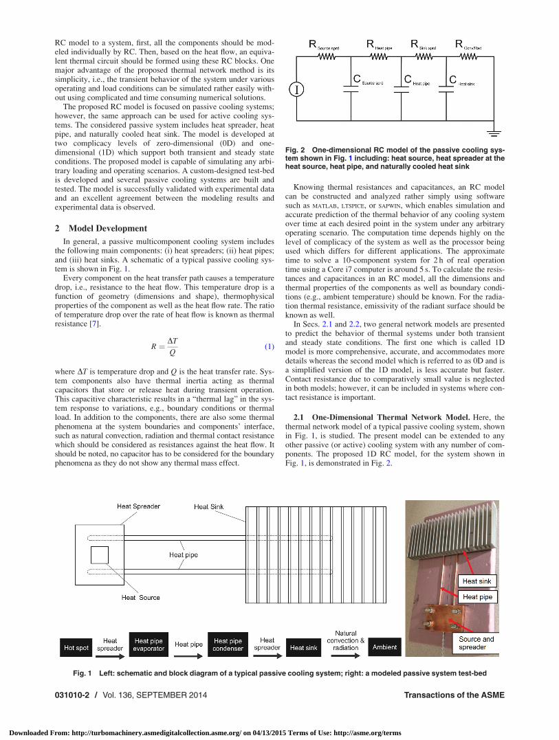
In general, a passive multicomponent cooling system includesthe following main components: (i) heat spreaders; (ii) heat pipes;and (iii) heat sinks. A schematic of a typical passive cooling sys-tem is shown in Fig. 1.
Every component on the heat transfer path causes a temperaturedrop, i.e., resistance to the heat flow. This temperature drop is afunction of geometry (dimensions and shape), thermophysicalproperties of the component as well as the heat flow rate. The ratioof temperature drop over the rate of heat flow is known as thermalresistance [7].
R ¼ DT
Q(1)
where DT is temperature drop and Q is the heat transfer rate. Sys-tem components also have thermal inertia acting as thermalcapacitors that store or release heat during transient operation.This capacitive characteristic results in a “thermal lag” in the sys-tem response to variations, e.g., boundary conditions or thermalload. In addition to the components, there are also some thermalphenomena at the system boundaries and components’ interface,such as natural convection, radiation and thermal contact resistancewhich should be considered as resistances against the heat flow. Itshould be noted, no capacitor has to be considered for the boundaryphenomena as they do not show any thermal mass effect.
Knowing thermal resistances and capacitances, an RC modelcan be constructed and analyzed rather simply using softwaresuch as MATLAB, LTSPICE, or SAPWIN, which enables simulation andaccurate prediction of the thermal behavior of any cooling systemover time at each desired point in the system under any arbitraryoperating scenario. The computation time depends highly on thelevel of complicacy of the system as well as the processor beingused which differs for different applications. The approximatetime to solve a 10-component system for 2 h of real operationtime using a Core i7 computer is around 5 s. To calculate the resis-tances and capacitances in an RC model, all the dimensions andthermal properties of the components as well as boundary condi-tions (e.g., ambient temperature) should be known. For the radia-tion thermal resistance, emissivity of the radiant surface should beknown as well.
In Secs. 2.1 and 2.2, two general network models are presentedto predict the behavior of thermal systems under both transientand steady state conditions. The first one which is called 1Dmodel is more comprehensive, accurate, and accommodates moredetails whereas the second model which is referred to as 0D and isa simplified version of the 1D model, is less accurate but faster.Contact resistance due to comparatively small value is neglectedin both models; however, it can be included in systems where con-tact resistance is important.
2.1 One-Dimensional Thermal Network Model. Here, thethermal network model of a typical passive cooling system, shownin Fig. 1, is studied. The present model can be extended to anyother passive (or active) cooling system with any number of com-ponents. The proposed 1D RC model, for the system shown inFig. 1, is demonstrated in Fig. 2.
Fig. 1 Left: schematic and block diagram of a typical passive cooling system; right: a modeled passive system test-bed
Fig. 2 One-dimensional RC model of the passive cooling sys-tem shown in Fig. 1 including: heat source, heat spreader at theheat source, heat pipe, and naturally cooled heat sink
031010-2 / Vol. 136, SEPTEMBER 2014 Transactions of the ASME
Downloaded From: http://turbomachinery.asmedigitalcollection.asme.org/ on 04/13/2015 Terms of Use: http://asme.org/terms
The capacitance of each component can be calculated usingEq. (2) which is the summation of all subcomponents’ capacities
C ¼X
i
ðmcpÞi ¼X
i
ðqcpVÞi (2)
where m is the mass of each part, cp is the thermal capacity, and qand V are the density and the volume of each part, respectively.However, the approach to define the resistance of each component
is different. In Secs. 2.1.1–2.1.4, a resistance model for each com-ponent is developed.
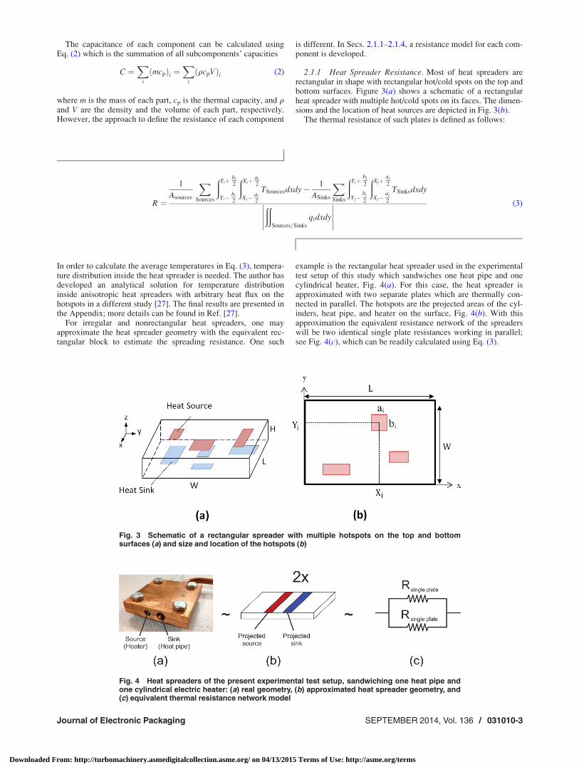
2.1.1 Heat Spreader Resistance. Most of heat spreaders arerectangular in shape with rectangular hot/cold spots on the top andbottom surfaces. Figure 3(a) shows a schematic of a rectangularheat spreader with multiple hot/cold spots on its faces. The dimen-sions and the location of heat sources are depicted in Fig. 3(b).
The thermal resistance of such plates is defined as follows:
R ¼
1
Asources
XSources
ðYiþbi
2
Yi�bi
2
ðXiþai
2
Xi�ai
2
TSourcesdxdy� 1
ASinks
XSinks
ðYjþbj
2
Yj�bj
2
ðXjþaj
2
Xj�aj
2
TSinksdxdy
ððSources=Sinks
qidxdy
����������
(3)
In order to calculate the average temperatures in Eq. (3), tempera-ture distribution inside the heat spreader is needed. The author hasdeveloped an analytical solution for temperature distributioninside anisotropic heat spreaders with arbitrary heat flux on thehotspots in a different study [27]. The final results are presented inthe Appendix; more details can be found in Ref. [27].
For irregular and nonrectangular heat spreaders, one mayapproximate the heat spreader geometry with the equivalent rec-tangular block to estimate the spreading resistance. One such
example is the rectangular heat spreader used in the experimentaltest setup of this study which sandwiches one heat pipe and onecylindrical heater, Fig. 4(a). For this case, the heat spreader isapproximated with two separate plates which are thermally con-nected in parallel. The hotspots are the projected areas of the cyl-inders, heat pipe, and heater on the surface, Fig. 4(b). With thisapproximation the equivalent resistance network of the spreaderswill be two identical single plate resistances working in parallel;see Fig. 4(c), which can be readily calculated using Eq. (3).
Fig. 3 Schematic of a rectangular spreader with multiple hotspots on the top and bottomsurfaces (a) and size and location of the hotspots (b)
Fig. 4 Heat spreaders of the present experimental test setup, sandwiching one heat pipe andone cylindrical electric heater: (a) real geometry, (b) approximated heat spreader geometry, and(c) equivalent thermal resistance network model
Journal of Electronic Packaging SEPTEMBER 2014, Vol. 136 / 031010-3
Downloaded From: http://turbomachinery.asmedigitalcollection.asme.org/ on 04/13/2015 Terms of Use: http://asme.org/terms
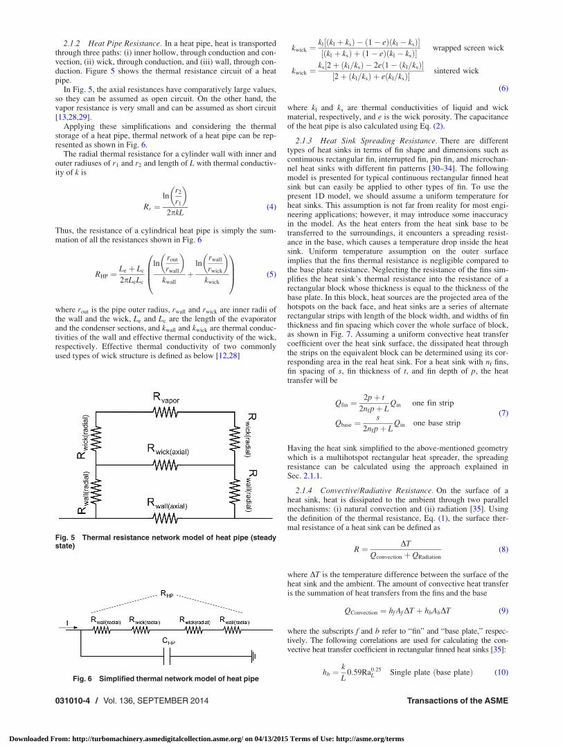
2.1.2 Heat Pipe Resistance. In a heat pipe, heat is transportedthrough three paths: (i) inner hollow, through conduction and con-vection, (ii) wick, through conduction, and (iii) wall, through con-duction. Figure 5 shows the thermal resistance circuit of a heatpipe.
In Fig. 5, the axial resistances have comparatively large values,so they can be assumed as open circuit. On the other hand, thevapor resistance is very small and can be assumed as short circuit[13,28,29].
Applying these simplifications and considering the thermalstorage of a heat pipe, thermal network of a heat pipe can be rep-resented as shown in Fig. 6.
The radial thermal resistance for a cylinder wall with inner andouter radiuses of r1 and r2 and length of L with thermal conductiv-ity of k is
Rr ¼ln
r2
r1
� �
2pkL(4)
Thus, the resistance of a cylindrical heat pipe is simply the sum-mation of all the resistances shown in Fig. 6
RHP ¼Le þ Lc
2pLeLc
lnrout
rwall
� �
kwall
þln
rwall
rwick
� �
kwick
0BB@
1CCA (5)
where rout is the pipe outer radius, rwall and rwick are inner radii ofthe wall and the wick, Le and Lc are the length of the evaporatorand the condenser sections, and kwall and kwick are thermal conduc-tivities of the wall and effective thermal conductivity of the wick,respectively. Effective thermal conductivity of two commonlyused types of wick structure is defined as below [12,28]
kwick ¼kl½ðkl þ ksÞ � ð1� eÞðkl � ksÞ�½ðkl þ ksÞ þ ð1� eÞðkl � ksÞ�
wrapped screen wick
kwick ¼ks½2þ ðkl=ksÞ � 2eð1� ðkl=ksÞ�½2þ ðkl=ksÞ þ eðkl=ksÞ�
sintered wick
(6)
where kl and ks are thermal conductivities of liquid and wickmaterial, respectively, and e is the wick porosity. The capacitanceof the heat pipe is also calculated using Eq. (2).
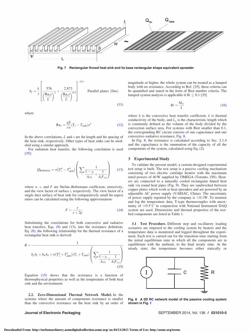
2.1.3 Heat Sink Spreading Resistance. There are differenttypes of heat sinks in terms of fin shape and dimensions such ascontinuous rectangular fin, interrupted fin, pin fin, and microchan-nel heat sinks with different fin patterns [30–34]. The followingmodel is presented for typical continuous rectangular finned heatsink but can easily be applied to other types of fin. To use thepresent 1D model, we should assume a uniform temperature forheat sinks. This assumption is not far from reality for most engi-neering applications; however, it may introduce some inaccuracyin the model. As the heat enters from the heat sink base to betransferred to the surroundings, it encounters a spreading resist-ance in the base, which causes a temperature drop inside the heatsink. Uniform temperature assumption on the outer surfaceimplies that the fins thermal resistance is negligible compared tothe base plate resistance. Neglecting the resistance of the fins sim-plifies the heat sink’s thermal resistance into the resistance of arectangular block whose thickness is equal to the thickness of thebase plate. In this block, heat sources are the projected area of thehotspots on the back face, and heat sinks are a series of alternaterectangular strips with length of the block width, and widths of finthickness and fin spacing which cover the whole surface of block,as shown in Fig. 7. Assuming a uniform convective heat transfercoefficient over the heat sink surface, the dissipated heat throughthe strips on the equivalent block can be determined using its cor-responding area in the real heat sink. For a heat sink with nf fins,fin spacing of s, fin thickness of t, and fin depth of p, the heattransfer will be
Qfin ¼2pþ t
2nfpþ LQin one fin strip
Qbase ¼s
2nfpþ LQin one base strip
(7)
Having the heat sink simplified to the above-mentioned geometrywhich is a multihotspot rectangular heat spreader, the spreadingresistance can be calculated using the approach explained inSec. 2.1.1.
2.1.4 Convective/Radiative Resistance. On the surface of aheat sink, heat is dissipated to the ambient through two parallelmechanisms: (i) natural convection and (ii) radiation [35]. Usingthe definition of the thermal resistance, Eq. (1), the surface ther-mal resistance of a heat sink can be defined as
R ¼ DT
Qconvection þ QRadiation
(8)
where DT is the temperature difference between the surface of theheat sink and the ambient. The amount of convective heat transferis the summation of heat transfers from the fins and the base
QConvection ¼ hf Af DT þ hbAbDT (9)
where the subscripts f and b refer to “fin” and “base plate,” respec-tively. The following correlations are used for calculating the con-vective heat transfer coefficient in rectangular finned heat sinks [35]:
hb ¼k
L0:59Ra0:25
L Single plate base plateð Þ (10)
Fig. 5 Thermal resistance network model of heat pipe (steadystate)
Fig. 6 Simplified thermal network model of heat pipe
031010-4 / Vol. 136, SEPTEMBER 2014 Transactions of the ASME
Downloaded From: http://turbomachinery.asmedigitalcollection.asme.org/ on 04/13/2015 Terms of Use: http://asme.org/terms
hf ¼k
s
576
Rass
L
� �2þ 2:873
Rass
L
� �0:5
26664
37775
�0:5
Parallel plates finsð Þ
(11)
where
Rax ¼gb�aðTs � TambÞx3 (12)
In the above correlations, L and s are fin length and fin spacing ofthe heat sink, respectively. Other types of heat sinks can be mod-eled using a similar approach.
For radiation heat transfer, the following correlation is used[35]:
QRadiation ¼ r T4s � T4
amb
� � Xi
1
1� ei
Aieiþ 1
AiFi1
0BB@
1CCA (13)
where r, e, and F are Stefan–Boltzmann coefficient, emissivity,and the view factor of surface i, respectively. The view factor of asingle duct surface of heat sink for comparatively small fin aspectratios can be calculated using the following approximation:
F ¼ s
sþ 2p(14)
Substituting the correlations for both convective and radiativeheat transfers, Eqs. (9) and (13), into the resistance definition,Eq. (8), the following relationship for the thermal resistance of arectangular heat sink is derived:
R¼ 1
hf Af þ hbAbþr T2s þT2
amb
� �ðTsþTambÞ
Xi
1
1� ei
Aieiþ 1
AiFi1
0BB@
1CCA
(15)
Equation (15) shows that the resistance is a function ofthermophysical properties as well as the temperature of both heatsink and the environment.
2.2. Zero-Dimensional Thermal Network Model. In thesystems where the amount of components resistance is smallerthan the convective resistance on the heat sink by an order of
magnitude or higher, the whole system can be treated as a lumpedbody with no resistance. According to Ref. [35], these criteria canbe quantified and stated in the form of Biot number criteria. Thelumped system analysis is applicable if Bi � 0:1 [35]
Bi ¼ hLc
k(16)
where h is the convective heat transfer coefficient, k is thermalconductivity of the body, and Lc is the characteristic length whichis commonly defined as the volume of the body divided by theconvection surface area. For systems with Biot smaller than 0.1,the corresponding RC circuit consists of one capacitance and oneconvective–radiative resistance, Fig. 8.
In Fig. 8, the resistance is calculated according to Sec. 2.1.4and the capacitance is the summation of the capacity of all thecomponents of the system, calculated using Eq. (2).
3 Experimental Study
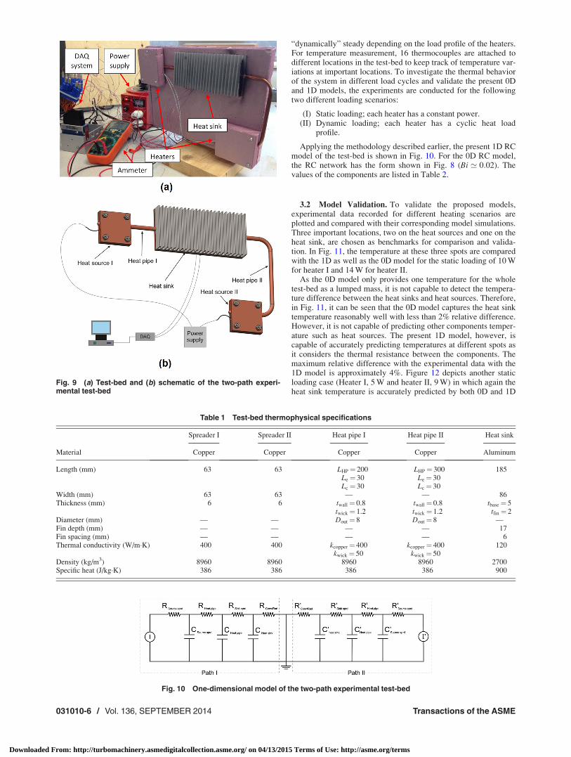
To validate the present model, a custom-designed experimentaltest setup is built. The test setup is a passive cooling mechanismconsisting of two electric cartridge heaters with the maximumrated powers of 40 W supplied by OMEGA (Toronto, ON). Heat-ers are connected to a naturally cooled rectangular finned heatsink via round heat pipes (Fig. 9). They are sandwiched betweencopper plates which work as heat spreaders and are powered by anadjustable AC power supply (VARIAC, China). The uncertaintyof power supply reported by the company is 60:1W. To monitorand log the temperature data, T-type thermocouples with uncer-tainty of 60:5�C in conjunction with National Instrument DAQsystem are used. Dimensions and thermal properties of the test-bed components are listed in Table 1.
3.1 Test Procedure. Different step and oscillatory loadingscenarios are imposed to the cooling system by heaters and thetemperature data is monitored and logged throughout the experi-ment. Each test is carried out for the transition time starting fromthe initial equilibrium state in which all the components are inequilibrium with the ambient, to the final steady state. At thesteady state, the temperature becomes either statically or
Fig. 7 Rectangular finned heat sink and its base rectangular shape equivalent spreader
Fig. 8 A 0D RC network model of the passive cooling systemshown in Fig. 1
Journal of Electronic Packaging SEPTEMBER 2014, Vol. 136 / 031010-5
Downloaded From: http://turbomachinery.asmedigitalcollection.asme.org/ on 04/13/2015 Terms of Use: http://asme.org/terms
“dynamically” steady depending on the load profile of the heaters.For temperature measurement, 16 thermocouples are attached todifferent locations in the test-bed to keep track of temperature var-iations at important locations. To investigate the thermal behaviorof the system in different load cycles and validate the present 0Dand 1D models, the experiments are conducted for the followingtwo different loading scenarios:
(I) Static loading; each heater has a constant power.(II) Dynamic loading; each heater has a cyclic heat load
profile.
Applying the methodology described earlier, the present 1D RCmodel of the test-bed is shown in Fig. 10. For the 0D RC model,the RC network has the form shown in Fig. 8 (Bi ’ 0:02). Thevalues of the components are listed in Table 2.
3.2 Model Validation. To validate the proposed models,experimental data recorded for different heating scenarios areplotted and compared with their corresponding model simulations.Three important locations, two on the heat sources and one on theheat sink, are chosen as benchmarks for comparison and valida-tion. In Fig. 11, the temperature at these three spots are comparedwith the 1D as well as the 0D model for the static loading of 10 Wfor heater I and 14 W for heater II.
As the 0D model only provides one temperature for the wholetest-bed as a lumped mass, it is not capable to detect the tempera-ture difference between the heat sinks and heat sources. Therefore,in Fig. 11, it can be seen that the 0D model captures the heat sinktemperature reasonably well with less than 2% relative difference.However, it is not capable of predicting other components temper-ature such as heat sources. The present 1D model, however, iscapable of accurately predicting temperatures at different spots asit considers the thermal resistance between the components. Themaximum relative difference with the experimental data with the1D model is approximately 4%. Figure 12 depicts another staticloading case (Heater I, 5 W and heater II, 9 W) in which again theheat sink temperature is accurately predicted by both 0D and 1D
Table 1 Test-bed thermophysical specifications
Spreader I Spreader II Heat pipe I Heat pipe II Heat sink
Material Copper Copper Copper Copper Aluminum
Length (mm) 63 63 LHP¼ 200 LHP¼ 300 185Le¼ 30 Le¼ 30Lc¼ 30 Lc¼ 30
Width (mm) 63 63 — — 86Thickness (mm) 6 6 twall¼ 0.8 twall¼ 0.8 tbase¼ 5
twick¼ 1.2 twick ¼ 1.2 tfin¼ 2Diameter (mm) — — Dout¼ 8 Dout¼ 8 —Fin depth (mm) — — — — 17Fin spacing (mm) — — — — 6Thermal conductivity (W/m�K) 400 400 kcopper¼ 400 kcopper¼ 400 120
kwick¼ 50 kwick ¼ 50Density (kg/m3) 8960 8960 8960 8960 2700Specific heat (J/kg�K) 386 386 386 386 900
Fig. 9 (a) Test-bed and (b) schematic of the two-path experi-mental test-bed
Fig. 10 One-dimensional model of the two-path experimental test-bed
031010-6 / Vol. 136, SEPTEMBER 2014 Transactions of the ASME
Downloaded From: http://turbomachinery.asmedigitalcollection.asme.org/ on 04/13/2015 Terms of Use: http://asme.org/terms
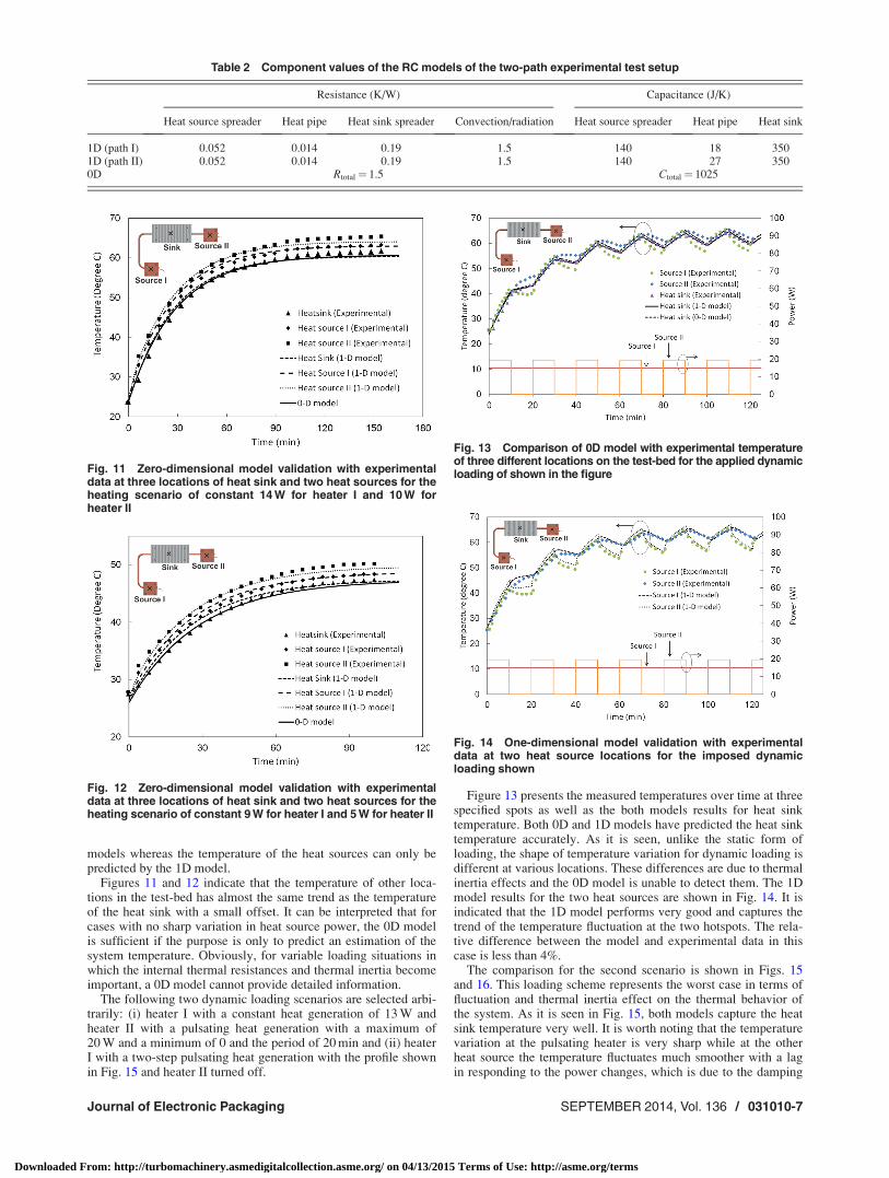
models whereas the temperature of the heat sources can only bepredicted by the 1D model.
Figures 11 and 12 indicate that the temperature of other loca-tions in the test-bed has almost the same trend as the temperatureof the heat sink with a small offset. It can be interpreted that forcases with no sharp variation in heat source power, the 0D modelis sufficient if the purpose is only to predict an estimation of thesystem temperature. Obviously, for variable loading situations inwhich the internal thermal resistances and thermal inertia becomeimportant, a 0D model cannot provide detailed information.
The following two dynamic loading scenarios are selected arbi-trarily: (i) heater I with a constant heat generation of 13 W andheater II with a pulsating heat generation with a maximum of20 W and a minimum of 0 and the period of 20 min and (ii) heaterI with a two-step pulsating heat generation with the profile shownin Fig. 15 and heater II turned off.
Figure 13 presents the measured temperatures over time at threespecified spots as well as the both models results for heat sinktemperature. Both 0D and 1D models have predicted the heat sinktemperature accurately. As it is seen, unlike the static form ofloading, the shape of temperature variation for dynamic loading isdifferent at various locations. These differences are due to thermalinertia effects and the 0D model is unable to detect them. The 1Dmodel results for the two heat sources are shown in Fig. 14. It isindicated that the 1D model performs very good and captures thetrend of the temperature fluctuation at the two hotspots. The rela-tive difference between the model and experimental data in thiscase is less than 4%.
The comparison for the second scenario is shown in Figs. 15and 16. This loading scheme represents the worst case in terms offluctuation and thermal inertia effect on the thermal behavior ofthe system. As it is seen in Fig. 15, both models capture the heatsink temperature very well. It is worth noting that the temperaturevariation at the pulsating heater is very sharp while at the otherheat source the temperature fluctuates much smoother with a lagin responding to the power changes, which is due to the damping
Table 2 Component values of the RC models of the two-path experimental test setup
Resistance (K/W) Capacitance (J/K)
Heat source spreader Heat pipe Heat sink spreader Convection/radiation Heat source spreader Heat pipe Heat sink
1D (path I) 0.052 0.014 0.19 1.5 140 18 3501D (path II) 0.052 0.014 0.19 1.5 140 27 3500D Rtotal¼ 1.5 Ctotal¼ 1025
Fig. 11 Zero-dimensional model validation with experimentaldata at three locations of heat sink and two heat sources for theheating scenario of constant 14 W for heater I and 10 W forheater II
Fig. 12 Zero-dimensional model validation with experimentaldata at three locations of heat sink and two heat sources for theheating scenario of constant 9 W for heater I and 5 W for heater II
Fig. 13 Comparison of 0D model with experimental temperatureof three different locations on the test-bed for the applied dynamicloading of shown in the figure
Fig. 14 One-dimensional model validation with experimentaldata at two heat source locations for the imposed dynamicloading shown
Journal of Electronic Packaging SEPTEMBER 2014, Vol. 136 / 031010-7
Downloaded From: http://turbomachinery.asmedigitalcollection.asme.org/ on 04/13/2015 Terms of Use: http://asme.org/terms
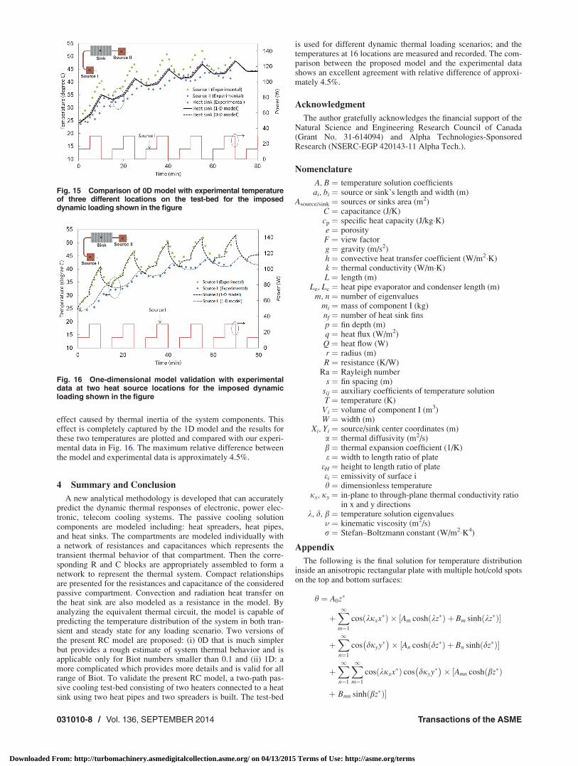
effect caused by thermal inertia of the system components. Thiseffect is completely captured by the 1D model and the results forthese two temperatures are plotted and compared with our experi-mental data in Fig. 16. The maximum relative difference betweenthe model and experimental data is approximately 4.5%.
4 Summary and Conclusion
A new analytical methodology is developed that can accuratelypredict the dynamic thermal responses of electronic, power elec-tronic, telecom cooling systems. The passive cooling solutioncomponents are modeled including: heat spreaders, heat pipes,and heat sinks. The compartments are modeled individually witha network of resistances and capacitances which represents thetransient thermal behavior of that compartment. Then the corre-sponding R and C blocks are appropriately assembled to form anetwork to represent the thermal system. Compact relationshipsare presented for the resistances and capacitance of the consideredpassive compartment. Convection and radiation heat transfer onthe heat sink are also modeled as a resistance in the model. Byanalyzing the equivalent thermal circuit, the model is capable ofpredicting the temperature distribution of the system in both tran-sient and steady state for any loading scenario. Two versions ofthe present RC model are proposed: (i) 0D that is much simplerbut provides a rough estimate of system thermal behavior and isapplicable only for Biot numbers smaller than 0.1 and (ii) 1D: amore complicated which provides more details and is valid for allrange of Biot. To validate the present RC model, a two-path pas-sive cooling test-bed consisting of two heaters connected to a heatsink using two heat pipes and two spreaders is built. The test-bed
is used for different dynamic thermal loading scenarios; and thetemperatures at 16 locations are measured and recorded. The com-parison between the proposed model and the experimental datashows an excellent agreement with relative difference of approxi-mately 4.5%.
Acknowledgment
The author gratefully acknowledges the financial support of theNatural Science and Engineering Research Council of Canada(Grant No. 31-614094) and Alpha Technologies-SponsoredResearch (NSERC-EGP 420143-11 Alpha Tech.).
Nomenclature
A, B ¼ temperature solution coefficientsai, bi ¼ source or sink’s length and width (m)
Asource/sink ¼ sources or sinks area (m2)C ¼ capacitance (J/K)cp ¼ specific heat capacity (J/kg�K)e ¼ porosityF ¼ view factorg ¼ gravity (m/s2)h ¼ convective heat transfer coefficient (W/m2�K)k ¼ thermal conductivity (W/m�K)L ¼ length (m)
Le, Lc ¼ heat pipe evaporator and condenser length (m)m, n ¼ number of eigenvalues
mi ¼ mass of component I (kg)nf ¼ number of heat sink finsp ¼ fin depth (m)q ¼ heat flux (W/m2)Q ¼ heat flow (W)r ¼ radius (m)R ¼ resistance (K/W)
Ra ¼ Rayleigh numbers ¼ fin spacing (m)
sij ¼ auxiliary coefficients of temperature solutionT ¼ temperature (K)
Vi ¼ volume of component I (m3)W ¼ width (m)
Xi, Yi ¼ source/sink center coordinates (m)a ¼ thermal diffusivity (m2/s)b ¼ thermal expansion coefficient (1/K)e ¼ width to length ratio of plate
eH ¼ height to length ratio of plateei ¼ emissivity of surface ih ¼ dimensionless temperature
jx, jy ¼ in-plane to through-plane thermal conductivity ratioin x and y directions
k, d, b ¼ temperature solution eigenvalues� ¼ kinematic viscosity (m2/s)r ¼ Stefan–Boltzmann constant (W/m2�K4)
Appendix
The following is the final solution for temperature distributioninside an anisotropic rectangular plate with multiple hot/cold spotson the top and bottom surfaces:
h ¼ A0z�
þX1m¼1
cos kjxx�ð Þ � Am cosh kz�ð Þ þ Bm sinh kz�ð Þ½ �
þX1n¼1
cos djyy�� �
� An cosh dz�ð Þ þ Bn sinh dz�ð Þ½ �
þX1n¼1
X1m¼1
cos kjxx�ð Þ cos djyy�� �
� Amn cosh bz�ð Þ½
þ Bmn sinh bz�ð Þ�
Fig. 16 One-dimensional model validation with experimentaldata at two heat source locations for the imposed dynamicloading shown in the figure
Fig. 15 Comparison of 0D model with experimental temperatureof three different locations on the test-bed for the imposeddynamic loading shown in the figure
031010-8 / Vol. 136, SEPTEMBER 2014 Transactions of the ASME
Downloaded From: http://turbomachinery.asmedigitalcollection.asme.org/ on 04/13/2015 Terms of Use: http://asme.org/terms
where k, d, and b are eigenvalues and A and B coefficients aredefined in the form below:
k ¼ mpjx; d ¼ np
jye; b ¼
ffiffiffiffiffiffiffiffiffiffiffiffiffiffiffik2 þ d2
p
A0 ¼st
00
e¼ sb
00
e
Am ¼2
eksb
m0csch keHð Þ � stm0 coth keHð Þ
� �
An ¼2
edsb
0ncsch deHð Þ � st0n coth deHð Þ
� �
Amn ¼4
ebsb
mncsch beHð Þ � stmn coth beHð Þ
� �
Bm ¼2st
m0
ekBn ¼
2st0n
edBmn ¼
4stmn
eb
In which the auxiliary coefficients “s”s are
st or b00 ¼
ððt or b
q�iðx;yÞdx�dy�
st or bm0 ¼
ððt or b
q�iðx;yÞ � cos kjxx�ð Þdx�dy�
st or b0n ¼
ððt or b
q�iðx;yÞ � cos djyy�� �
dy�dx�
st or bmn ¼
ððt or b
q�iðx;yÞ � cos kjxx�ð Þ cos djyy�� �
dx�dy�
References
[1] Gurrum, S. P., Suman, S. K., Joshi, Y. K., and Fedorov, A. G., 2004, “ThermalIssues in Next-Generation Integrated Circuits,” IEEE Trans. Device Mater.Reliab., 4(4), pp. 709–714.
[2] McGlen, R. J., Jachuck, R., and Lin, S., 2004, “Integrated Thermal ManagementTechniques for High Power Electronic Devices,” App. Therm. Eng., 24(8–9), pp.1143–1156.
[3] Zuo, Z., Hoover, L. R., and Phillips, A. L., 2002, “Advanced Thermal Architecturefor Cooling of High Power Electronics,” IEEE Trans. Compon. Packag. Technol.,25(4), pp. 629–634.
[4] Wunderle, B., and Michel, B., 2006, “Progress in Reliability Research in theMicro and Nano Region,” Microelectron. Reliab., 46(9–11), pp. 1685–1694.
[5] Suhir, E., 2013, “Thermal Stress Failures in Electronics and Photonics: Physics,Modeling, Prevention,” J. Therm. Stresses, 36(6), pp. 537–563.
[6] Suhir, E., Shangguan, D., and Bechou, L., 2013, “Predicted Thermal Stresses ina Trimaterial Assembly With Application to Silicon-Based PhotovoltaicModule,” ASME J. Appl. Mech., 80(2), p. 021008.
[7] Kakac, S., and Yener, Y., 1993, “One-Dimensional Steady-State Heat Conduction,”Heat Conduction, 3rd ed., Taylor & Francis, Washington, DC, pp. 45–93.
[8] Moghaddam, S., Rada, M., Shooshtari, A., Ohadi, M., and Joshi, Y., 2003,“Evaluation of Analytical Models for Thermal Analysis and Design of Elec-tronic Packages,” Microelectron. J., 34(3), pp. 223–230.
[9] Luo, X., Mao, Z., Liu, J., and Liu, S., 2011, “An Analytical Thermal ResistanceModel for Calculating Mean Die Temperature of a Typical BGA Packaging,”Thermochim. Acta, 512(1–2), pp. 208–216.
[10] Liu, S., Leung, B., Neckar, A., Memik, S. O., Memik, G., and Hardavellas, N.,2011, “Hardware/Software Techniques for DRAM Thermal Management,”IEEE 17th International Symposium on High Performance Computer Architec-ture (HPCA), San Antonio, TX, February 12–16, pp. 515–525.
[11] Zhao, R., Gosselin, L., Fafard, M., and Ziegler, D. P., 2013, “Heat Transfer inUpper Part of Electrolytic Cells: Thermal Circuit and Sensitivity Analysis,”Appl. Therm. Eng., 54(1), pp. 212–225.
[12] El-Nasr, A. A., and El-Haggar, S. M., 1996, “Effective Thermal Conductivityof Heat Pipes,” Heat Mass Transfer, 32(1–2), pp. 97–101.
[13] Zuo, J., and Faghri, A., 1998, “A Network Thermodynamic Analysis of theHeat Pipe,” Int. J. Heat Mass Transfer, 41(11), pp. 1473–1484.
[14] Shabgard, H., and Faghri, A., 2011, “Performance Characteristics of CylindricalHeat Pipes With Multiple Heat Sources,” Appl. Therm. Eng., 31(16), pp.3410–3419.
[15] Romary, F., and Caldeira, A., 2011, “Thermal Modelling to Analyze the Effectof Cell Temperature on PV Modules Energy Efficiency,” 14th European Con-ference on Power Electronics and Applications (EPE 2011), Birmingham, UK,August 30–September 1.
[16] Del Valle, P. G., and Atienza, D., 2011, “Emulation-Based Transient ThermalModeling of 2D/3D Systems-on-Chip With Active Cooling,” Microelectron. J.,42(4), pp. 564–571.
[17] Barcella, M., Huang, W., Skadron, K., and Stan, M., 2002, “Architecture-LevelCompact Thermal R-C Modeling,” Department of Electrical and Computer En-gineering, University of Virginia, Charlottesville, VA, Technical Report No.CS-2002-20.
[18] Stan, M. R., Skadron, K., Barcella, M., Huang, W., Sankaranarayanan, K., andVelusamy, S., 2003, “HotSpot: A Dynamic Compact Thermal Model at theProcessor-Architecture Level,” Microelectron. J., 34(12), pp. 1153–1165.
[19] Magnone, P., Fiegna, C., Greco, G., Bazzano, G., Rinaudo, S., and Sangiorgi,E., 2013, “Numerical Simulation and Modeling of Thermal Transient in SiliconPower Devices,” Solid-State Electron., 88, pp. 69–72.
[20] Cova, P., Bernardoni, M., Delmonte, N., and Menozzi, R., 2011, “DynamicElectro-Thermal Modeling for Power Device Assemblies,” Microelectron.Reliab., 51(9–11), pp. 1948–1953.
[21] L�opez-Walle, B., Gauthier, M., and Chaillet, N., 2010, “Dynamic Modelling forThermal Micro-Actuators Using Thermal Networks,” Int. J. Therm. Sci.,49(11), pp. 2108–2116.
[22] Miana, M., and Cort�es, C., 2010, “Transient Thermal NetworkModeling Applied to Multiscale Systems. Part II: Application to an ElectronicControl Unit of an Automobile,” IEEE Trans. Adv. Packag., 33(4), pp.938–952.
[23] Miana, M., and Cort�es, C., 2010, “Transient Thermal Network ModelingApplied to Multiscale Systems. Part I: Definition and Validation,” IEEE Trans.Adv. Packag., 33(4), pp. 924–937.
[24] Ramallo-Gonz�alez, A. P., Eames, M. E., and Coley, D. A., 2013, “LumpedParameter Models for Building Thermal Modelling: An Analytic Approach toSimplifying Complex Multi-Layered Constructions,” Energy Build., 60, pp.174–184.
[25] Buonomano, A., and Palombo, A., 2014, “Building Energy Performance Analysisby an In-House Developed Dynamic Simulation Code: An Investigation for Dif-ferent Case Studies,” Appl. Energy, 113, pp. 788–807.
[26] Athienitis, A., Kalogirou, S. A., and Candanedo, L., 2012, “Modeling and Sim-ulation of Passive and Active Solar Thermal Systems,” Comprehensive Renew-able Energy, Vol. 3: Solar Thermal Systems: Components and Applications,Elsevier, Ltd., Amsterdam, Netherlands, pp. 357–417.
[27] Gholami, A., and Bahrami, M., 2014, “Spreading Resistance in AnisotropicRectangular Plates With Multiple Heat Sources and Sinks,” 10th InternationalConference on Heat Transfer, Fluid Mechanics, and Thermodynamics, Orlando,FL, July 14–16.
[28] Ferrandi, C., Iorizzo, F., Mameli, M., Zinna, S., and Marengo, M., 2013,“Lumped Parameter Model of Sintered Heat Pipe: Transient Numerical Analysisand Validation,” Appl. Therm. Eng., 50(1), pp. 1280–1290.
[29] Zhu, N., and Vafai, K., 1999, “Analysis of Cylindrical Heat Pipes Incorporatingthe Effects of Liquid-Vapor Coupling and Non-Darcian Transport—A ClosedForm Solution,” Int. J. Heat Mass Transfer, 42(18), pp. 3405–3418.
[30] Mostafavi, G., 2013, “Effect of Fin Interruptions on Natural Convection HeatTransfer From a Rectangular Interrupted Single-Wall,” ASME Paper No.IPACK2013-73129.
[31] Dede, E., 2012, “Optimization and Design of a Multipass Branching Micro-channel Heat Sink for Electronics Cooling,” ASME J. Electron. Packag.,134(4), p. 041001.
[32] Xie, G., and Liu, J., 2012, “Analysis of Flow and Thermal Performance of aWater-Cooled Transversal Wavy Microchannel Heat Sink for Chip Cooling,”ASME J. Electron. Packag., 134(4), p. 041010.
[33] Xie, G., Liu, J., and Liu, Y., “Comparative Study of Thermal Performance ofLongitudinal and Transversal-Wavy Microchannel Heat Sinks for ElectronicCooling,” ASME J. Electron. Packag., 135(2), p. 021008.
[34] Xie, G., Zhang, F., Sund�en, B., and Zhang, W., 2014, “Constructal Design andThermal Analysis of Microchannel Heat Sinks With Multistage Bifurcations inSingle-Phase Liquid Flow,” Appl. Therm. Eng., 62(2), pp. 791–802.
[35] Incropera, F., DeWitt, D., Bergrnan, T., and Lavine, A. S., 2007, Fundamentalsof Heat and Mass Transfer, 6th ed., Wiley, Hoboken, NJ, pp. 559–780.
Journal of Electronic Packaging SEPTEMBER 2014, Vol. 136 / 031010-9
Downloaded From: http://turbomachinery.asmedigitalcollection.asme.org/ on 04/13/2015 Terms of Use: http://asme.org/terms