January 15, 2002

A New Algorithm for Scan Conversionof a General Ellipse

c©2002, C. Bond. All rights reserved.

1 Overview

This document contains a derivation of the equations for a general ellipse andimplementation details for a new scan conversion algorithm. The algorithmis developed for raster display applications, although its incremental steppingproperty makes it also suitable for use by plotters.

In the following paragraphs, certain properties of ellipses are developed, an-alyzed and applied to the drawing problem. Difficult cases are identified andsolved by a new algorithm which will be explained in some detail.

The basic incremental algorithms used to plot segments of the ellipse are notparticularly original. They are derived from a straightforward analysis ofthe general ellipse equation using midpoint criteria. However, the publishedstrategies used for moving from one plotted segment to the next will fail insome common circumstances. It is these pathological conditions which areidentified and solved in this paper.

Some other important papers on related subjects are: Aken [2], Bresen-ham [1], and Pitteway [3]. Foley [4] has a detailed discussion and code forthe general ellipse, pp.951-961.1

2 The General Ellipse

A standard form for general conics which includes ellipses is:

Ax2 +By2 + 2Cxy +Dx+ Ey + F = 0 (1)

In this equation, the coefficients of the x and y terms, D and E, representtranslation of the ellipse in the x, y plane. This equation can be simplified for

1References appear at the end of this paper.

1

our purposes by translating the center of the ellipse to the origin, eliminatingthe terms D and E

Ax2 +By2 + 2Cxy + F = 0 (2)

since the process of translation is easily deferred until plot time. This reducesthe problem to that of an origin-centered ellipse.

For ellipses with C = 0, the axes are aligned with the x, y coordinate axes.Otherwise there is an angle between the axes of the ellipse and the coordinateaxes. For any angle, the axes of the ellipse are perpendicular to each other.

Typically, an ellipse would be specified by the length of its major axis, thelength of its minor axis, and the angle that the major axis makes with thecoordinate system x axis. It is convenient to take the length of the major axisas 2a where a is the distance from the center of the ellipse to one end of themajor axis. Similarly, the length of the minor axis will be taken as 2b. Theangle from the positive x axis measured counterclockwise to the major axisof the ellipse will be designated θ. This angle will sometimes be referred to asthe rotation angle. We will use these conventions in the following treatment.

3 Basic Strategy

For this particular application, we begin by transforming the ellipse equationinto a more convenient form. We then calculate values for certain criticallocations along the ellipse perimeter, and derive incremental methods forplotting arc segments between these critical points.

Note that when plotting circles an 8-way symmetry reduces the calculationto that of a single octant. For axis aligned ellipses, there is 4-way symmetry,but for ellipses at arbitrary angles we will have to content ourselves with2-way symmetry.

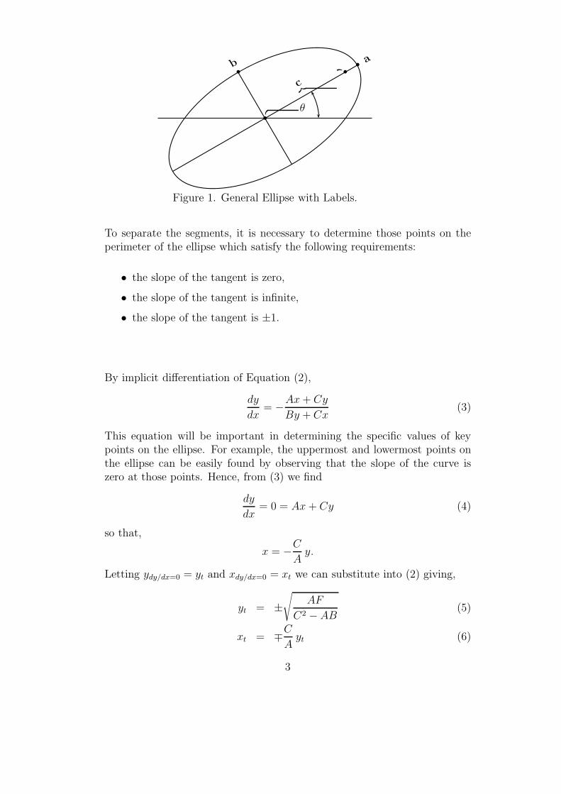
Figure 1. shows a general ellipse with a, b, and θ identified. Refer to theappendix for the relations between the coefficients A, B, C, F and the givenquantities a, b, and θ.

Incremental curve generation is best performed by breaking the curve intosegments consisting of arcs whose slopes are confined to a single octant.By this decomposition, it is possible to step along the x or y direction ateach iteration, and update the coordinate for the other direction using somecontrol variable.

2

θb

bb b

ab

︷

︸︸

︷

c

Figure 1. General Ellipse with Labels.

To separate the segments, it is necessary to determine those points on theperimeter of the ellipse which satisfy the following requirements:

• the slope of the tangent is zero,

• the slope of the tangent is infinite,

• the slope of the tangent is ±1.

By implicit differentiation of Equation (2),

dy

dx= −Ax+ Cy

By + Cx(3)

This equation will be important in determining the specific values of keypoints on the ellipse. For example, the uppermost and lowermost points onthe ellipse can be easily found by observing that the slope of the curve iszero at those points. Hence, from (3) we find

dy

dx= 0 = Ax+ Cy (4)

so that,

x = −C

Ay.

Letting ydy/dx=0 = yt and xdy/dx=0 = xt we can substitute into (2) giving,

yt = ±√

AF

C2 −AB(5)

xt = ∓C

Ayt (6)

3

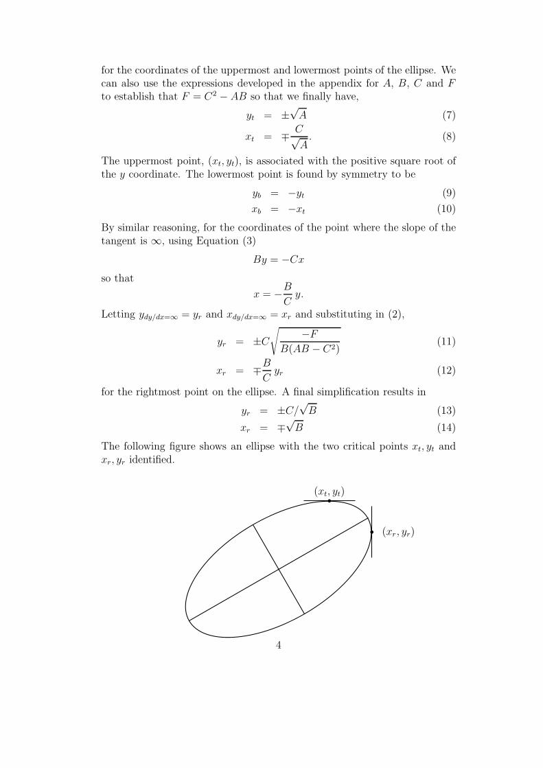
for the coordinates of the uppermost and lowermost points of the ellipse. Wecan also use the expressions developed in the appendix for A, B, C and Fto establish that F = C2 − AB so that we finally have,

yt = ±√A (7)

xt = ∓ C√A. (8)

The uppermost point, (xt, yt), is associated with the positive square root ofthe y coordinate. The lowermost point is found by symmetry to be

yb = −yt (9)

xb = −xt (10)

By similar reasoning, for the coordinates of the point where the slope of thetangent is ∞, using Equation (3)

By = −Cx

so that

x = −B

Cy.

Letting ydy/dx=∞= yr and xdy/dx=∞

= xr and substituting in (2),

yr = ±C

√

−F

B(AB − C2)(11)

xr = ∓B

Cyr (12)

for the rightmost point on the ellipse. A final simplification results in

yr = ±C/√B (13)

xr = ∓√B (14)

The following figure shows an ellipse with the two critical points xt, yt andxr, yr identified.

b

b

(xt, yt)

(xr, yr)

4

A complete list of the equations for all critical points required (right half ofellipse) is,

(xt, yt) = (− C√A,√A)

(xtr, ytr) = (B − C√

A +B − 2C,

A− C√A+B − 2C

)

(xr, yr) = (√B,− C√

B)

(xbr, ybr) = (B + C√

A +B + 2C,− A+ C√

A+B + 2C)

(xb, yb) = (C√A,−

√A)

By restricting the range of each segment so that its slope remains in the sameoctant, we can reduce the number of choices for the next point to two. Thisis done by choosing arc segments which are terminated by the critical pointswhere the slope of the tangent is 0, ∞ or ±1.

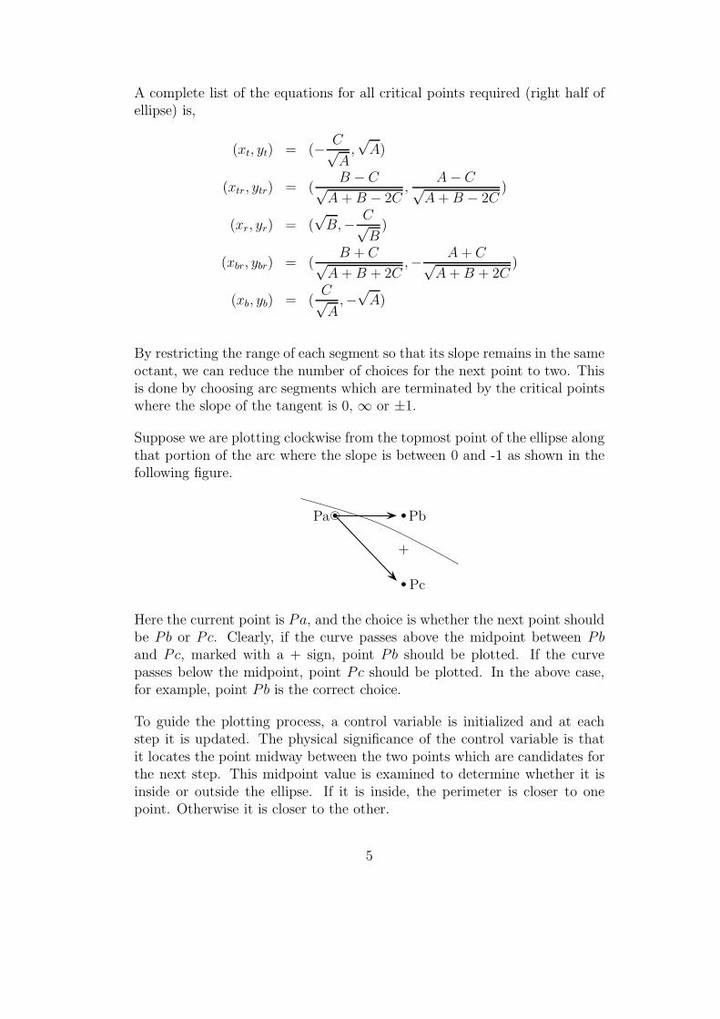
Suppose we are plotting clockwise from the topmost point of the ellipse alongthat portion of the arc where the slope is between 0 and -1 as shown in thefollowing figure.

bcb b

b

Pa Pb

Pc

+

Here the current point is Pa, and the choice is whether the next point shouldbe Pb or Pc. Clearly, if the curve passes above the midpoint between Pband Pc, marked with a + sign, point Pb should be plotted. If the curvepasses below the midpoint, point Pc should be plotted. In the above case,for example, point Pb is the correct choice.

To guide the plotting process, a control variable is initialized and at eachstep it is updated. The physical significance of the control variable is thatit locates the point midway between the two points which are candidates forthe next step. This midpoint value is examined to determine whether it isinside or outside the ellipse. If it is inside, the perimeter is closer to onepoint. Otherwise it is closer to the other.

5

4 The Control or Decision Variable

A derivation for the control variable equations will now be given. Only thecase for one segment will be considered, because the equations for othersegments are derived in a completely analogous manner.

If we have just plotted the ith point along the arc we just described at pointPa, we use the control variable to select the next point from Pb or Pc. Thecurrent point is somewhere on the arc from the topmost point of the ellipseto the point where the slope is -1, moving clockwise. The coordinates of thepoint are x, y. Then the value of the control variable is found by evaluatingthe ellipse equation at point midway between x+1, y and x+1, y−1. Simplysubstitute x+ 1 and y − 1/2 into the equation,

d = A(x+ 1)2 +B(y − 1/2)2 + 2C(x+ 1)(y − 1/2) + F

and if d is positive (outside the ellipse) choose Pc, otherwise choose Pb. Therare case in which di = 0 is a tossup, and is usually decided in favor of theoutermost point.

Since stepping along the perimeter is always done incrementally, it is possibleto precalculate di for the starting point of the arc, and update it with simplequantities at each step. Expressions for the update quantities can be derivedby examining the difference between the expression for di and di+1, wheredi+1 represents one of two possible cases.

At any point, xi, yi, in this segment, the value of the expression for the ellipseat the midpoint between Pb and Pc is,

f(x, y) = Ax2 +By2 + 2Cxy + F

di = f(xi + 1, yi − 1/2)

di = A(xi + 1)2 +B(yi − 1/2)2 + 2C(xi + 1)(yi − 1/2) + F

di = Ax2

i +By2i + 2Cxiyi + F

+(2A− C)xi + (2C − B)yi + A− C +B/4

If di ≤ 0, the midpoint is on or inside the ellipse and the next point should bePb. In that case the control variable di should be updated to di+1 is follows.

di+1 = f(xi+1 + 1, yi+1 − 1/2)

di+1 = f(xi + 2, yi − 1/2)

di+1 = A(xi+1 + 1)2 +B(yi+1 − 1/2)2

+2C(xi+1 + 1)(yi+1 − 1/2) + F

di+1 = di + 2Axi+1 + 2Cyi+1 + A− C

6

If di > 0, the midpoints is on or outside the ellipse and the next point shouldbe Pc.

di+1 = f(xi+1 + 1, yi+1 − 1/2)

di+1 = f(xi + 2, yi − 3/2)

di+1 = Ax2

i +By2i + 2Cxiyi + F

(4A− 3C)xi + (4C − 3B)yi + 4A− 6C + 9B/4

di+1 = di + 2(A− C)xi+1 + 2(C −B)yi+1 + A− C

To summarize the steps required to plot a give segment,

1. initialize the control variables,

2. plot the current best choice for (xi, yi),

3. use di to determine the next point,

4. update xi, yi and di appropriately,

5. repeat 2-4 until the chosen segment termination criteria is met.

This process is repeated for each segment. Since an origin centered generalellipse exhibits symmetry across the origin, we may plot two points in step2 of the above algorithm. The second point is found by reversing the signsof xi and yi.

For previously published algorithms, the termination of a segment is signaledby monitoring the slope of the tangent. When that slope passes through ±1,0 or ∞ a segment switch takes place.

5 A Plotting Problem and a New Solution

5.1 The Problem

The basic plotting strategy described above is sound — for most ellipses.However, if the aspect ratio (ratio of major to minor axis) of an ellipse islarge, sharp corners occur at the extreme points of the ellipse near the endsof the major axis. These corners correspond to regions of rapidly changingslope and it is quite possible for the slope computed at one point to be

7

totally inappropriate for determining the next step. Here we have a subpixelanomaly which requires special handling.

As stated earlier, previously published plotting strategies plot incrementallyfrom one region to the next, where the boundary between the regions isdetermined by detecting the point at which the slope equals 0, ∞ or ±1.At such a decision point the plotting algorithm switches to the next region.Unfortunately, for ellipses with large aspect ratios, it is possible for the curveto completely turn through one or more regions within a single pixel distance.When this happens the updated control variable is incorrect and the plotmay wander far from its intended course. This renders the plotting strategyuseless.

5.2 The Solution

Our solution is to precompute the coordinates of the critical points and storethem for reference. These points locate the boundaries of the arc segments ina definitive and unambiguous manner. Note that for narrow ellipses severalcritical points may cluster in a region consisting of a few adjacent pixels,or even a single pixel. This is the condition that defeats slope controlledalgorithms.

A stable plotting algorithm can be devised, however, by simply plotting eacharc from its start to the next critical point, rather than plotting until someslope criteria is met. When the next critical point is within a single pixeldistance, we simply plot it and advance to the next region. If the criticalpoint following this is identical to or adjacent to the current critical point,we skip the next segment entirely and just plot the critical point. Similarly,if any successive critical point is within a single pixel distance, we plot itand skip that segment. No ‘breakaway’ conditions occur with this strategyand all points are plotted correctly. In short, instead of using the slope tocontrol the plotting process, we use the proximity of the current location toa well-defined critical point.

Ellipses with large aspect ratio will have two clusters of critical points, oneat each end of the major axis. Broad regions of relative flatness join theseclusters. It is important to ensure that when plotting along one flat side wenever step across the major axis and wander into the wrong region. Thiscondition can be prevented by forming the equation for the line representingthe major axis and testing pixels to verify that they stay on the correct side.

8

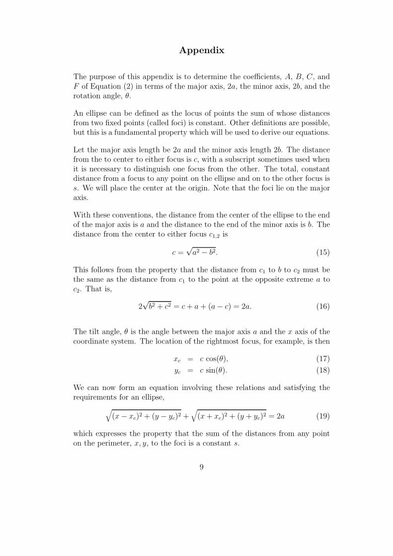
Appendix

The purpose of this appendix is to determine the coefficients, A, B, C, andF of Equation (2) in terms of the major axis, 2a, the minor axis, 2b, and therotation angle, θ.

An ellipse can be defined as the locus of points the sum of whose distancesfrom two fixed points (called foci) is constant. Other definitions are possible,but this is a fundamental property which will be used to derive our equations.

Let the major axis length be 2a and the minor axis length 2b. The distancefrom the to center to either focus is c, with a subscript sometimes used whenit is necessary to distinguish one focus from the other. The total, constantdistance from a focus to any point on the ellipse and on to the other focus iss. We will place the center at the origin. Note that the foci lie on the majoraxis.

With these conventions, the distance from the center of the ellipse to the endof the major axis is a and the distance to the end of the minor axis is b. Thedistance from the center to either focus c1,2 is

c =√a2 − b2. (15)

This follows from the property that the distance from c1 to b to c2 must bethe same as the distance from c1 to the point at the opposite extreme a toc2. That is,

2√b2 + c2 = c+ a + (a− c) = 2a. (16)

The tilt angle, θ is the angle between the major axis a and the x axis of thecoordinate system. The location of the rightmost focus, for example, is then

xc = c cos(θ), (17)

yc = c sin(θ). (18)

We can now form an equation involving these relations and satisfying therequirements for an ellipse,

√

(x− xc)2 + (y − yc)2 +√

(x+ xc)2 + (y + yc)2 = 2a (19)

which expresses the property that the sum of the distances from any pointon the perimeter, x, y, to the foci is a constant s.

9

To determine the values of A, B, C, and F in Equation (2), we must expand(19) in powers of x and y.

The urge to clear out radicals, nurtured by past experience, is irresistible.Begin by rearranging Equation (19), squaring and simplifying.

√

(x+ xc)2 + (y + yc)2 = 2a−√

(x− xc)2 + (y − yc)2 (20)

xxc + yyc = a2 − a√

(x− xc)2 + (y − yc)2 (21)

Again rearranging, squaring and simplifying,

a√

(x− xc)2 + (y − yc)2 = a2 − (xxc + yyc) (22)

a2x2 + a2(x2

c + y2c ) + a2y2 = a4 + x2x2

c + 2xcycxy + y2y2c (23)

Collecting terms in powers of x and y yields,

(a2 − x2

c)x2 + (a2 − y2c )y

2 − 2xcycxy + a2(x2

c + y2c − a2) = 0.

Substituting c2 for x2c + y2c ,

(a2 − x2

c)x2 + (a2 − y2c )y

2 − 2xcycxy + a2(c2 − a2) = 0,

and, finally, replacing c2 − a2 with −b2, we have

(a2 − x2

c)x2 + (a2 − y2c )y

2 − 2xcycxy − a2b2 = 0. (24)

From Equations (2) and (24),

A = a2 − x2

c (25)

B = a2 − y2c (26)

C = −xcyc (27)

F = −a2b2 (28)

References

[1] J. E. Bresenham, “A Linear Algorithm for Incremental Digital Displayof Digital Arcs”, Comm. ACM, Vol 20, No. 2, Feb. 1977, pp. 100-106.

[2] Jerry R. Van Aken, “Efficient Ellipse-Drawing Algorithm”, Texas In-

struments Incorporated.

10

[3] M. Pitteway, “Algorithm for Drawing Ellipses or Hyperbolae with aDigital Plotter”, C omputer J., Vol 10, No. 3, Nov. 1967, pp.282-289.

[4] James D. Foley, et al.,“Computer Graphics, Principles and Practice,”Addison-Wesley Publishing Company, 1997.

11