A Neuro�Dynamic Programming Approach toRetailer Inventory Management�

Benjamin Van Royyz

Dimitri P� Bertsekasz

Yuchun Leey

John N� Tsitsiklisz

yUnica Technologies� Inc�Lincoln North

Lincoln� MA �����

and

zLaboratory for Information and Decision SystemsMassachusetts Institute of Technology

Cambridge� MA �����

�This material is based upon work supported by the National Science Foundation un�

der award number �������� Any opinions� ndings� and conclusions or recommendations

expressed in this publication are those of the authors and do not necessarily reect the

views of the National Science Foundation�

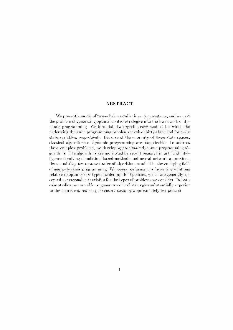
ABSTRACT

We present a model of twoechelon retailer inventory systems� and we castthe problem of generating optimal control strategies into the framework of dynamic programming� We formulate two specic case studies� for which theunderlying dynamic programming problems involve thirtythree and fortysixstate variables� respectively� Because of the enormity of these state spaces�classical algorithms of dynamic programming are inapplicable� To addressthese complex problems� we develop approximate dynamic programming algorithms� The algorithms are motivated by recent research in articial intelligence involving simulation�based methods and neural network approximations� and they are representative of algorithms studied in the emerging eldof neurodynamic programming� We assess performance of resulting solutionsrelative to optimized s�type � order�up�to�� policies� which are generally accepted as reasonable heuristics for the types of problems we consider� In bothcase studies� we are able to generate control strategies substantially superiorto the heuristics� reducing inventory costs by approximately ten percent�

�

� Introduction

Many important problems in operations research involve sequential decisionmaking under uncertainty� or stochastic control� Dynamic programming �Bertsekas� ����� provides an omnipotent framework for studying such problems� aswell as a suite of algorithms for computing optimal decision policies� Unfortunately� the overwhelming computational requirements of these algorithmsrender them inapplicable to most realistic problems� As a result� complexstochastic control problems that arise in the real world are usually addressedusing drastically simplied analyses and�or heuristics�

An exciting new alternative that is more closely tied to the sound framework of dynamic programming is being developed in the emerging eld ofneurodynamic programming �Bertsekas and Tsitsiklis� ������ This approachmakes use of ideas from articial intelligence involving simulation�based algorithms and functional approximation techniques such as neural networks�The outcome is a methodology for approximating dynamic programming solutions without demanding the associated computational requirements�

Over the past few years� neurodynamic programming methods have generated several notable success stories� Examples include a program that playsBackgammon at the world champion level �Tesauro� ������ an elevator dispatcher that is more e�cient than several heuristics employed in practice�Crites and Barto� ������ and an approach to job shop scheduling �Zhangand Dietterich� ������ Additional case studies reported by Bertsekas andTsitsiklis ������ further demonstrate signicant promise for neurodynamicprogramming� However� neurodynamic programming is a young eld� andthe algorithms that have been most successful in applications are not fullyunderstood at a theoretical level� Furthermore� there is a large conglomeration of algorithms proposed by researchers in the eld� and each one iscomplicated and parameterized by many values that must be selected by auser� It is unclear which algorithms and parameter settings will work on aparticular problem� and when a method does work� it is still unclear whichingredients were actually necessary for success� Because of this� application ofneurodynamic programming often requires trial and error� in a long processof parameter tweaking and experimentation�

In this paper� we describe work directed towards developing a streamlined neurodynamic programming approach for optimizing performance of

�

retailer inventory systems �Nahmias and Smith� ������ This is the problemof ordering and positioning retailer inventory at warehouses and stores in order to meet customer demands while simultaneously minimizing storage andtransportation costs� This problem can also be viewed as a simple examplefrom the broad class of multiechelon inventory control problems that has received signicant attention in the eld of supplychain management �Lee andBillington� ������

The remainder of this paper is organized as follows� The next sectionprovides an overview of the research and results obtained� Section � describes in detail the model of retailer inventory systems used in this study�while Section � discusses the use of s�type policies in this model� Dynamicprogramming and neurodynamic programming are presented in Sections �and �� respectively� Rather than presenting the methodologies in full generality� the material in these sections is customized to the purposes of retailerinventory management� Experimental results are discussed in Section �� Section � contains some concluding remarks� Finally� formal state equations areprovided in the appendix as a mathematically precise description of our retailer inventory system model�

� Overview of Research

Rather than simply describing the nal results obtained at the end of thisresearch� we attempt in this paper to present some of the obstacles that wereencountered and how they were overcome� We hope that this will lead to abetter perspective on the stateoftheart in neurodynamic programming� aswell as the potential di�culty of applying the methodology� In this section�we overview the steps taken in this research and the results obtained at theend of the process� Subsequent sections provide a far more detailed accountof what we discuss here�

In formulating a model of retailer inventory systems� we attempted tore�ect the complexities that make the problem di�cult� However� we didnot attempt to capture all aspects of the problem that may be required formodeling a realworld retailer inventory system� The objective of this studywas to establish the viability of neurodynamic programming as an e�ectiveapproach to optimizing retailer inventory systems� We expect that successdemonstrated on the models we present will generalize to more realistic models�

To gauge the e�cacy of the neurodynamic programming algorithms de

�

veloped in this study� performance was compared with optimized s�typepolicies �i�e�� orderupto� policies�� which have been the most commonlyadopted approach in past research concerning optimization of retailer inventory systems �Nahmias and Smith� ����� Nahmias and Smith� ������ Thedetails of this heuristic method are discussed in Section ��

In choosing and customizing neurodynamic programming algorithms forthe purpose of retailer inventory management� an e�ort was made to minimizethe complexity of the methods� Only ingredients deemed critical to successwere included� and we avoided many of the frills� that make for additionalparameters to be tweaked� We initially selected two neurodynamic programming algorithms and specialized them for the purposes of retailer inventorymanagement� The two algorithms were approximate policy iteration and anonline temporaldi�erence method �Bertsekas and Tsitsiklis� ������

In solving a stochastic control problem like that of retailer inventory management� neurodynamic programming algorithms approximate the problem�scosttogo function by tuning parameters of an approximation architecture�Appropriate approximation architectures must be chosen for the problem athand� In this research� we chose to employ linear and multilayer perceptron�neural network� architectures coupled with the extraction of features pertinent to the problem� We describe the chosen features and architectures inmore detail later in this paper�

In an initial set of experiments� we analyzed only a very simple retailerinventory system� This system consisted of one warehouse and one store� andthe underlying stochastic control problem involved only three state variables�A multilayer perceptron architecture� using the raw state variables as input features� was coupled with the neurodynamic programming algorithmsto solve the problem� Unfortunately� the neurodynamic programming algorithms led to control strategies that performed far worse than an optimizeds�type policy�

Extensive experimentation and a study of where the neurodynamic programming algorithms were failing on this simple problem led to a modicationin the online temporaldi�erence algorithm� This involved adding an elementof active exploration to the workings of the algorithm� the details of which willbe described in a later section� The resulting algorithm generated approximations using the multilayer perceptron architecture that yielded performanceessentially equivalent to the heuristic approach�

It is not surprising that the heuristic and the neurodynamic programmingapproach delivered similar levels of performance on the rst problem� Inparticular� since the problemwas so simple� bothmethods were probably near

�

optimal� A second set of experiments was performed on a more complex casestudy� This new problem involved a central warehouse and ten stores withsubstantial transportation delays� The underlying stochastic control problemthis time involved �� state variables� A set of �� features was selected basedon the given problem� and a featurebased linear architecture was tried withthe online temporaldi�erence algorithm� This combination was successful�generating policies that reduced costs by about ten percent over the cost ofan optimized heuristic policy�

To see if this result could be further improved� we tried two variations ofthe approach� First� we replaced the featurebased linear architecture witha featurebased multilayer perceptron architecture �using the same features��However� this did not lead to performance superior to the linear case� Asecond variation involved increasing the degree of exploration in the onlinetemporal di�erence method� Again� this did not improve performance�

We tested the neurodynamic programming approach on an additionalproblem of even greater complexity� This time� the underlying stochasticcontrol problem involved �� state variables� Again� the combination of afeaturebased linear architecture and the online temporal di�erence method�with active exploration� led to costs about ten percent lower than the heuristic�

In the nal analysis� neurodynamic programming proved to be successfulin solving two complex retailer inventory management problems� To summarize the results obtained� we reiterate some key points�

�� The straightforward approximate policy iteration algorithms that wereemployed in the initial stages of this research do not work in their initialsimple form�

�� The online temporal di�erence method with active exploration� coupledwith a feature�based linear architecture� consistently cut costs by aboutten percent �over a well�accepted heuristic approach� on two di�erentcomplex retailer inventory management problems�

�� Given the chosen features� using a multilayer perceptron instead of thelinear architecture did not lead to improved performance�

�� Increasing the degree of exploration in the temporaldi�erence algorithmdid not lead to improved performance �just a small amount of exploration seemed to be required to make the huge di�erence in performanceover having no exploration at all��

�

warehouse

stores

customerdemandsmanufactured

goods

special deliveries

Figure �� Schematic diagram of a retailer inventory system�

� A Model of Retailer Inventory Systems

In this section� we describe the model of retailer inventory systems used inthis study� The characteristics of this model are largely motivated by thestudies of �Nahmias and Smith� ����� and �Nahmias and Smith� ������ Thegeneral structure is illustrated in Figure � and involves several stages�

�� Transportation of products from manufacturers

�� Packaging and storage of products at a central warehouse

�� Delivery of products from the warehouse to stores

�� Fulllment of customer demands using either store or warehouse inventory

Demands materialize at each store during each time period� Each unit ofdemand can be viewed as a customer request for the product� If inventory isavailable at the store� it is used to meet ongoing demands� In the event of ashortage� the customer will� with a certain probability� be willing to wait fora special delivery from the warehouse� If the customer is in fact willing towait� the demand is lled by inventory from the warehouse �if it is available��

At the end of each day� the warehouse orders additional units of inventoryfrom the manufacturers� and the stores place orders to the warehouse� Thewarehouse manager lls store orders as much as possible given current levelsof inventory� As materials travel from manufacturers to the warehouse andfrom the warehouse to the stores� they are delayed by transportation times�

�

warehouse

stores

customerdemands

manufacturedgoods

Figure �� An illustration of the bu�ers in the retailer inventory system�

Coupled with the uncertainty of future demands� these delays create the needfor storage of inventory at stores�

The di�ering impact of inventory at the warehouse on costs and serviceperformance makes it desirable to also maintain stock there� For example�inventory stored at the warehouse provides a greater degree of �exibilitythan that maintained at a single store� In particular� inventory stored atthe warehouse can be used to ll special orders made by customers at anystore �for individual customers who are willing to wait�� and can also besent to any store in the advent of a shortage of goods� On the other hand� asurplus of inventory at one store cannot be used to compensate for a shortageat another� Furthermore� storage costs at stores are often higher than at thewarehouse�

In the remainder of this section� we present some technical details concerning aspects of the model we have described� In particular� we furtherdiscuss the dynamics of inventory �ow� the nature of the stochastic demandprocess� and the cost structure�

��� Dynamics of Inventory Flow

As illustrated in Figure �� inventory is stored at two stages� The warehouseholds reserves in anticipation of special orders and shipments to stores� whichmake up the second stage of inventory storage� There are delays in the transportation of stock from one stage to the next� and to simplify our discussion�we consider the delays to be multiples of a xed unit of time which we willtake to be a day� Hence� the model involves a dynamic system that evolvesin discrete time�

The delays in the inventory system are illustrated in Figure �� Each squarerepresents a bu�er where goods may be located at a particular point in time�

�

The movement of goods between bu�ers is synchronized by a single clock that ticks� once per day� Goods enter and exit bu�ers only at the clock ticks� Therow of bu�ers to the left of the warehouse bu�er are associated with delays inthe transportation of goods from a manufacturer to the warehouse� At eachclock tick� goods located in any one of these bu�ers moves one bu�er to theright� Similarly� the row of bu�ers to the left of each store bu�er is associatedwith delays in transporting goods from the warehouse to the store� Again�at each clock tick� goods proceed one bu�er to the right� as transportationprogresses�

The entrance of goods into the system and the movement of goods fromthe warehouse to transportation bu�ers are controlled by decisions of theinventory manager� which are made just prior to each tick� At each tick� aspecied quantity of goods �the warehouse order� enters the system at theleftmost bu�er� This quantity is limited by a production capacity as well asthe warehouse capacity� The amount ordered at any one time cannot exceedthe production capacity� and the total quantity of goods currently at andonroute to the warehouse cannot exceed the warehouse capacity�

Also at each tick� a specied quantity of goods are transferred from thewarehouse to the leftmost transportationbu�ers of specied stores� Of course�the total quantity of goods transfered here must be less than the amountavailable at the warehouse prior to the tick� Furthermore� at any time� thetotal quantity of goods currently at and onroute to any particular store canbe no greater than the store capacity�

Goods exit the system upon customer demand� At each tick� such demands arise at each of the stores� If the amount demanded at a particularstore is less than or equal to the quantity of inventory available just priorto the tick� the store�s inventory level is reduced by the demanded quantity�Otherwise� the store�s inventory is completely depleted� and each unsatisedcustomer is allowed the option to request a special delivery from the warehouse� In our model� each individual customer makes such a request with agiven probability� If a customer whose demand has not been satised by thestore does make such a request� and a unit of inventory is available� then thewarehouse inventory is decremented by one�

To be completely precise� we must specify the ordering of events thatoccur at each clock tick� First� goods ordered by the warehouse enter into thesystem� Second� goods are transferred from the warehouse to the appropriatetransportation bu�ers� Then� demands are lled as needed� Finally� goods intransportation bu�ers progress towards the right�

�

��� Demand Process

In the model� stochasticity arises from the uncertainty of future demands�In this research� the demands were modeled as random variables that areindependent and identically distributed through time and among di�erentstores� Each sample was generated as follows�

�� sample from a normal distribution with a given mean and a given standard deviation�

�� round o� this value to the closest integer�

�� take the maximum of zero and the resulting value�

��� Cost Structure

At each clock tick� a cost of operation is incurred by the retailer inventorysystem� The objective of the rm is to minimize these costs� on average� Thecost can be broken down into three categories� storage cost� shortage cost�and transportation cost� In this section� we describe how each of these costsare computed�

Storage costs are incurred at both the warehouse and the stores� At eachclock tick� the total quantity of inventory at stores is multiplied by a storecost of storage� and the quantity of inventory at the warehouse is multipliedby a warehouse cost of storage� The sum of these two products is the storagecost for that day�

Shortage costs are costs associated with unfullled demands� A customer�sdemand may be satised by inventory either at the store where the customeris located or the warehouse �if the customer opts for a special delivery�� Anycustomer whose demands are not lled by either of these two places incurs ashortage cost to the system�

Transportation costs in our model are associated only with special deliveries� In particular� each special delivery made to a customer incurs aparticular cost� Note that for special deliveries to be protable� the cost ofan unfullled unit of demand �i�e�� shortage cost� must be greater than thatof a special delivery�

��� Model Parameters

Now that we have described the dynamics of the model in detail� it may beuseful to enumerate the model parameters� Values must be assigned to these

�

parameters in order to make the model behavior commensurate with that ofa specic manifestation of a retailer inventory system� The list follows�

�� Number of stores

�� Delay to stores

�� Delay to warehouse

�� Production capacity

�� Warehouse capacity

�� Store capacity

�� Probability of customer waiting

�� Cost of special delivery

�� Warehouse storage cost

��� Store storage cost

��� Mean demand

��� Demand standard deviation

��� Shortage cost

� Heuristic Policies

A heuristic policy for controlling the retailer inventory system was implemented and used as a baseline for comparison against neurodynamic programming approaches� The type of heuristic used is known as an stype� or orderupto�� policy and is accepted as a reasonable approach to problemformulations that have independent identically distributed demands� like theone we have proposed� Examples of research where such policies are the focusof study are discussed in �Nahmias and Smith� ����� and include �Nahmiasand Smith� ������

The s�type policy we implemented is parameterized by two values� awarehouse orderupto level and a store orderupto level� Essentially� ateach time step the inventory manager tries to order inventory such that all

�

inventory at and expected to arrive at the warehouse is equal to the warehouse orderupto level and all the inventory at or expected to arrive at anyparticular store is equal to the store orderupto level�

Although the main idea is simple� the details of how store orders are generated by the heuristic policy are tedious� First� a desired order� equal to thedi�erence between the store orderupto level and the total of inventory currently at the store and inventory currently onroute to the store is computedfor each store� If all desired orders can be lled by the inventory currentlyavailable at the warehouse� then they are� Otherwise� all inventory at thewarehouse is sent to stores� and the preference among stores is decided in away that always maximizes the minimum among stores of the total of currentinventory and inventory onroute to a store�

Once the store orders have been computed� we compute the total of inventory currently at the warehouse and all inventory onroute to the warehouse�less the total of store orders� If the di�erence between this quantity and thewarehouse orderupto level is less than the production capacity� then thewarehouse order is set equal to this di�erence� Otherwise� the warehouseorder is equal to the production capacity�

Note that we have discussed only how the heuristic policy works givenspecied orderupto levels� but not how the orderupto levels are to bedetermined� In this research� the best orderupto levels were determinedby an exhaustive search� where the average cost associated with each pairof orderupto levels was assessed in a lengthy simulation� Note that anexhaustive search of this type would be computationally prohibitive if weallowed the stores to have di�erent orderupto levels� which would be calledfor if the stores had independent attributes �e�g�� di�erent transportationdelays��

� Dynamic Programming

Dynamic programming �DP� o�ers a very general framework for stochasticcontrol problems �Bertsekas� ������ In this section� we present a DP framework that is a bit di�erent from the standard� In particular� our setting issomewhat specialized to the retailer inventory problem and leads to moree�cient computational approaches in the context of neurodynamic programming �NDP�� We also present in detail the way in which we formulated theretailer inventory management problem in terms of this DP framework� Tomake the exposition of DP both brief and precise� we only discuss the case

��

involving systems that evolve over nite state spaces and in discrete time�Let S be the state space of a system of interest �each element corresponds

to a particular combination of inventory levels�� We associate two statesxt� yt � S to any nonnegative integer time t� We refer to xt as the predecision state� and yt as the postdecision state�� Furthermore� a decisionut that in�uences the system is selected from a nite set U at each time step�The state evolves according to two di�erence equations� xt�� � f��yt� wt�and yt � f��xt� ut�� where f� and f� are some functions describing the systemdynamics and wt is a random noise term taken from a xed distribution�independent from all information available up to time t� There is a costg�yt� wt� associated with the system a�ected by a noise term wt while thepostdecision state is yt�

A policy is a mapping � � S �� U that determines a decision as a functionof predecision state� i�e�� ut � ��xt�� The goal in stochastic control is to selectan optimal policy �i�e�� one that minimizes longterm costs�� We express thelongterm cost to be minimized as the expectation of a discounted innitesum of future costs� as a function of an initial postdecision state� i�e��

J��y� � E

��Xt��

�tg�yt� wt�jy� � y� �

��

Here� � � ��� �� is a discount factor and J��y� denotes the expected longtermcost given that the system starts in postdecision state y and is controlled bya policy �� An optimal policy �� is one that minimizes J� simultaneouslyfor all initial postdecision states� and the function J�

�

� known as the valuefunction� is denoted by J��

A well known result in dynamic programming is that the value functionsatises Bellman�s equation� which in our formulation� takes on the form

J��y� � Ew

�g�y� w�� � �J�f��y� w��

��

where �J is given by�J�x� � min

u�UJ��f��x� u���

Furthermore� a policy �� is optimal if and only if it satises

���x� � argminu�U

J��f��x� u���

Note that� using this expression� we can generate an optimal policy based ona value function J� that is dened only over the post�decision states� If this

��

function is available� there is no need for the function �J � which denes valuesfor pre�decision states�

In principle� an optimal policy can be found by rst numerically solvingBellman�s equation and then computing the optimal policy using the resultingvalue function� However� this requires computation and storage of J��y� foreach postdecision state� which is generally infeasible given the enormity ofstate spaces for practical problems�

We now describe how the retailer inventory management problem wasformulated in terms of the DP framework we have described� First of all� thestate of the retailer system is described by a vector in which each componentcorresponds to a bu�er �see Figure ��� At any time� each state variable takesa value equal to the quantity of goods currently located at the correspondingbu�er� Hence� the number of state variables �components of the state vector�is equal to one plus the warehouse transportation delay plus the number ofstores times one plus the store transportation delay� Note that the size of thestate space here grows exponentially with the number of state variables� andtherefore quickly becomes intractable�

Each decision ut corresponds to a vector of store and warehouse ordersduring the tth time step� The decision ut must be made on the basis of thepredecision state xt� Given the predecision state xt and the decision ut�the postdecision state yt is generated deterministically� This involves theentrance of goods ordered by the warehouse into the leftmost bu�er and thetransition of goods ordered by stores from the warehouse bu�er to appropriatetransportation bu�ers�

The post decision state yt is transformed as customer demands are fullledand transportation progresses� The result of these transformations is thenext pre�decision state xt��� Note that the transition from yt to xt�� isin�uenced by stochastic demands� In the context of our DP formulation�demands correspond to the random noise term wt� The dynamics of thestate transitions can be inferred from the description of our retailer inventorysystem model� provided in Section �� Nevertheless� to enhance clarity� wepresent formal state equations in the appendix�

Costs g�yt� wt� are computed in a fairly straightforward manner as described in Section �� The discount factor used in our formulation was �����The reason is that policies will be evaluated in terms of average costs and setting the discount factor close to one makes the discounted problem resemblethe average cost problem�

��

FeatureState

FeatureVector

ParameterVector

Cost-To-GoExtractor

FunctionApproximator

Figure �� A feature�based approximation architecture�

� Neuro�Dynamic Programming

Dynamic programming o�ers a suite of algorithms for generating optimal control strategies� However� the overwhelming computational requirements associated with these algorithms render them inapplicable in practical situations�Due to a lack of other systematic approaches for dealing with such problems�simplied problemspecic analyses and heuristics have become the norm�Such analyses and heuristics often ignore much information that is important to e�ective decisionmaking� leading to control policies that are far fromoptimal� The recent emergence of neurodynamic programming puts forth anexciting new possibility� New and highly promising approaches to addressing complex stochastic control problems have been developed in this eld�These approaches focus on approximating solutions that would be generatedby dynamic programming� except in a computationally feasible manner�

The main idea in neurodynamic programming is to approximate the mapping J� � S �� � using an approximation architecture� An approximation architecture can be thought of as a function �J � S ��k �� �� NDP algorithmstry to nd a parameter vector r � �k such that the function �J��� r� closelyapproximates J��

In general� choosing an appropriate approximation architecture is a problem dependent task� In this research� we designed approximation architectures involving two stages� a feature extractor and a function approximator�see Figure ��� The feature extractor uses the postdecision state yt to compute a feature vector zt� The components of zt are values that we thoughtwere natural for capturing key information concerning states of the retailerinventory management problem� This feature vector was used as input to asecond stage� which involved a generic function approximator parameterized

��

by a vector r� Two types of function approximators were employed in thisresearch� linear approximators and the multilayer perceptron neural networkwith a linear output node� In the case of the linear approximator� all butone component of the parameter vector r correspond to coe�cients that aremultiplied by individual components of the feature vector� The remainingcomponent is a scalar o�set term� In the case of the multilayer perceptron�the parameter vector r stores the weights of the network connections�

In the remainder of this section� we describe the NDP algorithms that wereused to tune parameters of our approximation architectures� The features weused are described in Section �� The function approximators �linear andmultilayer perceptron� are well known� and we omit any detailed discussionabout them�

��� Approximate Policy Iteration

Approximate policy iteration is a generalization of policy iteration� a classicalalgorithm in dynamic programming� The policy iteration algorithm generatesa sequence �i of improving policies� The initial policy �� is usually chosento be some reasonable heuristic� and the cost function J�� associated withthe policy is computed �one value is computed for each state�� Then� a newpolicy �� is generated according to the equation

���x� � argminu�U

J���f��x� u���

The same procedure is iterated to generate subsequent policies� It is wellknown that for problems with a nite number of policies� �i is equal to ��

and J�i is equal to J� for su�ciently large i�In approximate policy iteration� instead of computing the cost function J�i

exactly at each iteration� the function is approximated by some architecture�J��� ri�� where ri is a parameter vector chosen to make �J��� ri� close to J�i �The subsequent policy is then generated via

�i���x� � argminu�U

�J�f��x� u�� ri��

There have been many methods used for approximating J�i in each ithpolicy iteration� A comprehensive survey is provided in �Bertsekas and Tsitsiklis� ������ In this research� we chose to use the online TD��� method�which at each iteration� e�ectively computes the parameter vector ri thatminimizes X

x�S

�i�x��J�i�x�� �J�x� ri�

���

��

where �i�x� stands for the relative frequency of occurrence of state x whenthe system is controlled by policy �i� We refer the reader to �Bertsekas andTsitsiklis� ����� for a detailed discussion of this method�

��� An On�Line Temporal�Di�erence Method

Variants of the temporaldi�erence algorithm �Sutton� ����� Tsitsiklis andVan Roy� ����� have been applied successfully to several large scale applications of NDP� Examples include a Backgammon player �Tesauro� ������an elevator dispatcher �Crites and Barto� ������ and a job shop schedulingmethod �Zhang and Dietterich� ������ The variants used in these applications bear signicant di�erences� and in this research project� we tried touse a simple algorithm that possessed what we felt were the most important properties� In this section� we present the algorithm in its initial form�This algorithmmay be viewed as an extreme form of optimistic approximatepolicy iteration�� as discussed in �Bertsekas and Tsitsiklis� ������ As mentioned in Section �� this algorithm was not successful until we added activeexploration� which is discussed in the next section�

The algorithm updates the parameter vector of an approximation architecture during each step of a single endless simulation� In particular� we startwith an arbitrary parameter vector r� and generate a sequence rt using thefollowing procedure�

�� Given the initial pre�decision state x� of the simulator� generate a control u� by letting

u� � argminu�U

�J�f��x�� u�� r���

�� Run the simulator using control u� to obtain the rst postdecision state

y� � f��x�� u���

�� More generally� at time t� run the simulator using control ut to obtainthe next predecision state

xt�� � f��yt� wt��

and the cost g�yt� wt��

�� Generate a control ut�� by letting

ut�� � argminu�U

�J�f��xt��� u�� rt��

��

�� Run the simulator using control ut�� to obtain the postdecision state

yt�� � f��xt��� ut����

�� Update the parameter vector via

rt�� � rt � �t

�g�yt� wt� � �J�yt��� rt�� �J�yt� rt�

�rr

�J�yt� rt��

where �t is a small step size parameter�

�� Return to step ����

��� Active Exploration

As we mentioned in the introduction� it was only after we added active exploration to the workings of the temporaldi�erence method that it performedwell� Note that the algorithm described in the previous section always updates the parameter vector to tune the approximate values �J�x� r� at states xvisited by the current policy� which in turn are determined by the parametervector r� In some sense� the exploration here is passive� i�e�� only states thatnaturally occur on the basis of the current approximation to the value function are visited� By active exploration� we refer to a mechanism that bringsabout some tendency to visit a larger range of states�

Except for the steps involving generation of control decisions� the temporaldi�erence algorithm that we used with active exploration follows the sameroutine as that without active exploration� In particular� the algorithm canbe described by the steps enumerated in the previous section� except with theequations of Steps ��� and ��� replaced by

u� � n� � argminu�U

�J�f��x�� u�� r���

andut�� � nt � argmin

u�U

�J�f��xt��� u�� rt��

respectively� where each nt is a noise term� Note that the only di�erence isthe addition of a noise term� The structure of the noise term is described ona casebycase basis in the next section�

��

� Results With the NDP Approach

In this section� we present the results obtained from applying the NDP approaches we developed to the retailer inventorymanagementproblem� Throughour development� much of which occurred in the process of experimentation�we arrived at an approach that was successful relative to the heuristic stypepolicies� To the extent of our experimentation� the method also proved to berobust to changes in problemspecics�

In this section� we present a relatively detailed account of our experimental results� Experiments were conducted using three di�erent problemsas test beds� each described in the following subsections with its associatedexperiments�

�� Initial Experiments With a Simple Problem

The rst set of experiments involved optimization of a very simple retailer inventory system� The purpose of these experiments was to debug the softwarepackages developed in the initial stages of research and also to ensure thatthe NDP methodologies worked reasonably well on a simple problem� beforemoving to complex situations�

The system included only one store in addition to the warehouse� Therewas no delay for goods ordered by the warehouse� and there was a delay ofonly one time unit between the warehouse and the store� There were therefore only three state variables involved �each corresponding to the quantityof goods within a bu�er�� The list of parameter settings for this problemare provided in the table below� Note that we also have provided the truemean and standard deviation of demands �recall from Section � that the meanand standard deviation parameters do not correspond to the true mean andstandard deviations of the resulting stochastic demands��

��

number of stores �

delay to stores �

delay to warehouse �

production capacity ��

warehouse capacity ��

store capacity ��

probability of customer waiting �

cost of special delivery ��

warehouse storage cost �

store storage cost �

mean demand �true mean� � �����

demand stdev �true stdev� � �����

shortage cost ��

As a baseline for comparison� we developed an stype policy� optimizingthe orderupto levels associated with the warehouse and store� Figure � illustrates how varying the orderupto levels a�ects the average cost of the policy�Each point on the graph is computed by averaging costs over a lengthy simulation� The optimal orderupto levels turned out to be �� for the warehouseand �� for the store� The corresponding average cost was �����

Several NDP algorithms were tried with a single approximation architecture� The architecture consisted of a multilayer perceptron with ten hiddennodes in a single hidden layer� Three features were used as input to the network� each a normalized version of one of the state variables� In particular�if the bu�er levels at a given point in time were bi� i � �� �� �� then the ithinput feature was given by

ci �bi � �bi�i

�

The �bi�s and �i�s were computed prior to execution of the NDP algorithmas follows� A large collection of �postdecision� states sampled while simulating the heuristic policy �with the optimal orderupto levels� was collected�From this data� each �bi was set equal to the sample mean of the ith statevariable� and each �i was set equal to the sample standard deviation of theith state variable�

The approximate policy iteration algorithm� in the form described in Section �� was tried on the problem� The s�type policy �with optimized orderupto levels� was used as the initial policy� This algorithm consistently generateda second policy that was far worse than the initial one�

��

010

2030

4050

0

10

20

30

40

50

50

100

150

200

250

300

350

store level

warehouse level

aver

age

cost

Figure �� Performance of the heuristic as a function of orderupto levels� Theoptimum levels was �� for the warehouse and �� for the store� With theselevels� the average cost was �����

Upon failure of the approximate policy iteration algorithm� experimentswere conducted using the online temporaldi�erence method� Again� onlypolicies that were far worse than the heuristic were generated�

Next� we tried adding a small degree of exploration to the online temporaldi�erence method� In particular� each time a decision was generated usingthe approximation architecture �J � a noise term was added to the decision�Recall that there are two decision variables� the warehouse order and thestore order� The noise term was generated by adding a unit normal randomvariable to each decision variable� rounding o� to the closest integer in eachcase� and then making sure the decision variables stayed within their limits�That is� if the noise term made a variable negative� the variable was set tozero� and if the noise term made a variable too large �e�g�� having a warehouseorder greater than the production capacity�� then the variable was set to itsmaximum allowable value�

With the extra exploration term� the online temporaldi�erence methodessentially matched the performance of the heuristic� Figure � displays theevolution of average cost as the algorithm progresses in tuning the parametersof the multilayer perceptron� in experiments performed both with and withoutactive exploration� In both cases� a step size �t � ���� was used for the rst�� ��� time steps� and a step size �t � ����� was used for the next �� ���

��

0 0.5 1 1.5 2 2.5 3 3.5 4

x 107

50

55

60

65

70

75

80

85

90

95

100

number of steps

aver

age

cost

ove

r pr

evio

us 1

0000

ste

ps

Figure �� A demonstration of the importance of exploration� The twoplots show the evolution of average cost using the online temporaldi�erencemethod with �lower plot� and without �higher plot� exploration� Each pointrepresents cost averaged over ten thousand consecutive time steps during theexecution of an algorithm�

time steps�Note that in the graph of Figure � associated with the exploratory version

of the algorithm� the average cost is computed during the execution of the algorithm� and is thus a�ected by the active exploration� In particular� a policybased on the nal approximate value function without any exploratory termshould perform better than the policy with active exploration �the explorationis there to improve the learning and discovery� process that the algorithmgoes through� rather than to improve performance of a policy at any giventime�� Indeed� a simulation employing a nonexploratory policy based on thenal approximate value function generated an average cost of ����� which wasslightly better than average costs sampled during execution of the exploratoryonline algorithm�

�� Case Study �

With the success of the online temporaldi�erence method on a simple problem� a subsequent set of experiments was conducted on a more complex testbed� The parameters used for the retailer inventory management problem of

��

this case study are given in the table below�

number of stores ��

delay to stores �

delay to warehouse �

production capacity ���

warehouse capacity ����

store capacity ���

probability of customer waiting ���

cost of special delivery �

warehouse storage cost �

store storage cost �

mean demand �true mean� � �����

demand stdev �true stdev� �� �����

shortage cost ��

Once again� an s�type heuristic policy was developed by optimizing overorderupto levels� Since the properties of all stores were identical� we assumed that the order uptolevels of all stores should be the same� and therewere again only two variables to optimize� a warehouse orderupto level anda store orderupto level� Figure � shows how the average cost of the system varies with these two variables� Each value in the graph was computedfrom a lengthy simulation� The optimal orderupto levels were ��� for thewarehouse and �� for each store� The corresponding average cost was �����

In the simple problem of the previous section� there were only two inventory sites for which orders had to be placed� In the more complex problem ofthis section� on the other hand� there are eleven inventory sites� and exhausting all possible combinations of orders that can be made for these eleven siteswould take too long� In particular� the minimizations carried out in steps��� and ��� of the online temporaldi�erence method would be essentiallyimpossible to carry out� Because of this� we constrained the decision spaceto a more manageable subset�

First of all� we represented decisions in terms of two variables� a warehouse order and a store orderupto level� Given particular values for the twovariables� the individual store orders would be set to exactly what the s�typepolicy described in Section � would set them to given the store orderuptolevel� Note� however� that unlike the case of the heuristic s�type policy� thestore orderuptolevel here is chosen at each time step� rather than taken tobe a xed constant�

��

010

2030

40

0

200

400

600

1000

2000

3000

4000

5000

6000

store level

warehouse level

aver

age

cost

Figure �� Performance of the heuristic as a function of orderupto levels�The optimum levels were ��� for the warehouse and �� for each of the stores�With these levels� the average cost was �����

To further accelerate execution of the online temporaldi�erence method�we limited the space of decisions considered at each time step to the setinvolving warehouse orders ranging from �� to ��� in increments of �� andstore orderupto levels ranging from � to �� in increments of �� There weretherefore a total of �� possible decisions considered at each time step� Theminimization in Step ��� of the temporaldi�erence algorithm was carried outby exhaustive enumeration of these �� possible decisions�

The approximation architectures employed in this case study involved theuse of the following �� features�

��� total inventory at stores��� total inventory to arrive at stores in one time step��� total inventory to arrive at stores in two time steps��� inventory at warehouse��� inventory to arrive at warehouse in one time step��� inventory to arrive at warehouse in two time steps��� inventory to arrive at warehouse in three time steps������� the squares of ���������� variance among stores of inventory levels

��

���� variance among stores of inventory levels plus inventory to arrive in onetime step���� variance among stores of inventory levels plus inventory to arrive withintwo time steps���� the product of ��� and ������� the product of ��� and the sum of ��� through ������� the sum of ��� through ��� times the sum of ��� through ������� the sum of ��� through ��� times the sum of ��� through ������� the product of ���� ���� and ���

By variance among stores �as in features ���� through ������ we meanthe average among stores of the square of the di�erence between quantitiesassociated with each store and the average of such quantities over the stores�

The feature values were normalized using an approach analogous to thatused in the context of the simple problem from the previous section� Inparticular� a data set was collected from simulations using the stype policy�and this data was used to compute means and standard deviations associatedwith each feature� These mean and standard deviation values were then usedas normalization parameters just as in the previous section�

For active exploration� noise terms were added to the decisions generatedusing the approximate value function at each step of the temporaldi�erencealgorithm� The way noise terms were added is completely analogous to themethod employed in the previous section� except that this time the noise termadded to the warehouse order involved a normal random variable with a meanof zero and a standard deviation of ve� Furthermore� the noise terms addedto the store orders were independent from one another�

We began by using a featurebased linear architecture with the featuresdescribed� We experimented with di�erent step sizes to better understandhow the temporaldi�erence method was working with this problem� Wefound that the performance tended to diverge with larger step sizes� andimproved at an extremely slow rate when the step sizes were reduced enoughto prevent divergence� Upon investigation of feature values� it was foundthat feature ���� was taking on values far larger than those that appearedwhen the system was controlled by the stype policy� Hence� we increased thestandard deviation parameter associated with this feature to scale its valuesdown signicantly� Once this was done� performance improved at a muchfaster rate upon execution of the temporaldi�erence algorithm�

Two variations on the initial architecture�algorithm were explored� Oneinvolved replacing the linear function approximator with a multilayer per

��

0 0.5 1 1.5 2 2.5 3 3.5 4 4.5

x 106

1000

1200

1400

1600

1800

2000

2200

2400

number of steps

aver

age

cost

ove

r pr

evio

us 5

000

step

s

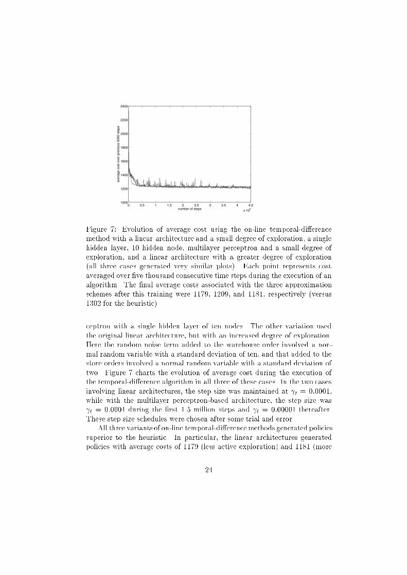
Figure �� Evolution of average cost using the online temporaldi�erencemethod with a linear architecture and a small degree of exploration� a singlehidden layer� �� hidden node� multilayer perceptron and a small degree ofexploration� and a linear architecture with a greater degree of exploration�all three cases generated very similar plots�� Each point represents costaveraged over ve thousand consecutive time steps during the execution of analgorithm� The nal average costs associated with the three approximationschemes after this training were ����� ����� and ����� respectively �versus���� for the heuristic��

ceptron with a single hidden layer of ten nodes� The other variation usedthe original linear architecture� but with an increased degree of exploration�Here the random noise term added to the warehouse order involved a normal random variable with a standard deviation of ten� and that added to thestore orders involved a normal random variable with a standard deviation oftwo� Figure � charts the evolution of average cost during the execution ofthe temporaldi�erence algorithm in all three of these cases� In the two casesinvolving linear architectures� the step size was maintained at �t � �������while with the multilayer perceptronbased architecture� the step size was�t � ������ during the rst ��� million steps and �t � ������� thereafter�These step size schedules were chosen after some trial and error�

All three variants of online temporaldi�erencemethods generated policiessuperior to the heuristic� In particular� the linear architectures generatedpolicies with average costs of ���� �less active exploration� and ���� �more

��

0 0.5 1 1.5 2 2.5

x 106

−0.04

−0.02

0

0.02

0.04

0.06

0.08

0.1

0.12

0.14

number of steps

valu

es o

f coe

ffici

ents

Figure �� Evolution of coe�cient values during training using the on�linetemporal �di�erence method with a linear architecture and a small degree ofexploration�

active exploration�� while the multilayer perceptron architecture led to anaverage cost of ����� Hence� the best policy cut costs by about ten percentrelative to the heuristic� Figure � charts the evolution of parameter valuesin the linear featurebased architecture as they were tuned by the onlinetemporal di�erence method with the lesser degree of exploration�

�� Case Study �

We tested the on�line temporal di�erence algorithm on an additional problemof even greater complexity than the previous one� The parameters for thisnew problem are given in the table below�

��

020

4060

80100

0

200

400

600

800

1000

1000

2000

3000

4000

5000

store level

warehouse level

aver

age

cost

Figure �� Performance of the heuristic as a function of orderupto levels�The optimum levels were ��� for the warehouse and �� for each of the store�With these levels� the average cost was �����

number of stores ��

delay to stores �

delay to warehouse �

production capacity ���

warehouse capacity ����

store capacity ���

probability of customer waiting ���

cost of special delivery �

warehouse storage cost �

store storage cost �

mean demand �true mean� � �����

demand stdev �true stdev� �� ������

shortage cost ��

Once again� an s�type heuristic policy was developed by optimizing overorderupto levels� Figure � shows how the average cost of the system varieswith the two orderupto levels� Each value in the graph was computed from alengthy simulation� The optimal orderupto levels were ��� for the warehouseand �� for each store� The corresponding average cost was �����

��

As in the previous section� decisions were represented in terms of twovariables� a warehouse order and a store orderupto level� This time� thedecision space was limited to warehouse orders ranging from �� to ��� in increments of �� and store orderupto levels ranging from � to �� in incrementsof �� for a total of �� possible decisions considered at each time step�

The approximation architectures employed in this case study involved theuse of the following �� features�

��� total inventory at stores��� total inventory to arrive at stores in one time step��� total inventory to arrive at stores in two time steps��� total inventory to arrive at stores in three time steps��� inventory at warehouse��� inventory to arrive at warehouse in one time step��� inventory to arrive at warehouse in two time steps��� inventory to arrive at warehouse in three time steps��� inventory to arrive at warehouse in four time steps���� inventory to arrive at warehouse in ve time steps�������� the squares of ����������� variance among stores of inventory levels���� variance among stores of inventory levels plus inventory to arrive in onetime step���� variance among stores of inventory levels plus inventory to arrive withintwo time steps���� variance among stores of inventory levels plus inventory to arrive withinthree time steps���� the product of ��� and ������� the product of ��� and the sum of ��� through ������� the sum of ��� through ���� times the sum of ��� through ������� the sum of ��� through ��� times the sum of ��� through ������� the product of ���� ���� and ����

The feature values were normalized using the same approach as in theprevious case study� except that this time� the scaling parameter associatedwith feature ��� was the one that needed to be increased�

Noise terms were once again added to the orders during execution of thetemporaldi�erence algorithm� The noise terms used here were exactly thesame as the smaller noise terms of the two tried in the previous section�

��

0 0.5 1 1.5 2 2.5

x 106

1200

1300

1400

1500

1600

1700

1800

1900

number of steps

aver

age

cost

ove

r pr

evio

us 5

000

step

s

Figure ��� Evolution of average cost using the online temporaldi�erencemethod with a linear architecture and a small degree of exploration� Eachpoint represents cost averaged over ve thousand consecutive time steps during the execution of an algorithm� The nal average cost associated withthe approximation scheme after this training �without exploration� was �����versus ���� for the heuristic��

We used a featurebased linear architecture with the features we havedescribed� Figure �� charts the evolution of average cost during the executionof the temporaldi�erence algorithm� The step size was �t � ������ duringthe rst million steps and �t � ������� thereafter�

Once again� the online temporaldi�erence method generated a policysuperior to the heuristic� The average cost was ����� a savings of almost tenpercent relative to the heuristic�s average cost of �����

Conclusions

Through this study� we have demonstrated that NDP can provide a viableapproach to advancing the stateoftheart in retailer inventory management�The method we have developed outperformed a wellaccepted heuristic approach in two case studies�

Though the problems we solved in this research were truly complex froma technical standpoint� not much e�ort was directed at ensuring that themodels re�ected all the practical issues inherent in realworld retailer invent

��

ory systems� Further research is required to translate the methods we havedeveloped into those that could be truly benecial in a realworld application�

Finally� it may be possible to improve the results obtained in this research�Alternative choices of architectures and algorithms may lead to further reductions in inventory costs� Also� since performance is measured in termsof average cost� formulating the problem in terms of average�cost �ratherthan discounted cost� dynamic programming and employing NDP algorithmsthat directly address such formulations may enhance performance� Such algorithms are discussed in �Bertsekas and Tsitsiklis� ����� and analyzed in�Abounadi et al�� ����� and �Tsitsiklis and Van Roy� ������

Acknowledgments

We would like to thank colleagues at Unica and the Laboratory for Information and Decision Systems for useful discussions� feedback� proof�reading�and help with various other matters� In particular� special thanks go to RubyKennedy� Bob Crites� and Steve Patek�

A State Equations

In this appendix� we formalize the retailer inventory system model by providing explicit state equations� The purpose here is to make our descriptionprecise using mathematical notation� We do not intend to generate a better intuitive understanding of the model dynamics� which have already beendiscussed at length in Section ��

Recall that� for each time t� there are associated pre�decision and post�decision states� denoted by xt and yt� respectively� Each post�decision stateis given by yt � f��xt� ut�� for some function f�� where ut is a decisionrepresenting orders placed at time t� On the other hand� each pre�decisionstate is given by xt�� � f��yt� wt�� for some function f�� where wt is a randomvariable representing demands that arise at time t� To formally dene thedynamics of the model� we will describe the structure of the state vectors xtand yt� the decisions ut� the random variables wt� and the system functionsf� and f��

A�� State Vectors

Both pre�decision and post�decision states represent quantities of inventorycontained in bu�ers of the system �see Figure ��� Suppose we have K stores

��

indexed by i � �� � � � � K� Let q��T be the quantity of inventory that is currentlybeing transported and will arrive at the warehouse in T days� Similarly� letqi�T be the quantity to arrive at the ith store in T days� We use q��� andq���� � � � � qK�� here to represent the current levels of inventory at the warehouseand the stores� Let Dw and Ds be the delays for transportation of goods tothe warehouse and from the warehouse to the stores� Then� a vector

x ��q���� � � � � q��Dw � q���� � � � � q��Ds� � � � � qK��� qK�Ds

�captures all relevant information concerning current inventory levels� Thevectors xt and yt take on this general structure�

A�� Decisions

We represent decisions by vectors of the form

ut ��a�� a�� � � � � aK

��

where a� denotes a warehouse order and a�� � � � � ak denote the store orders� Inorder to enforce that orders and inventory levels are positive and that storageand production capacities are not exceeded� several constraints are placed onthe decision space� Given a current pre�decision state

xt ��q���� � � � � q��Dw � q���� � � � � q��Ds� � � � � qK��� qK�Ds

��

the constraints on ut are captured by the following inequalities�

ai � �� i � f�� � � � � Kg�

a� Cp�

KXi��

ai q����

a� Cw �DwXT��

q��T �KXi��

ai�

ai Cs �DsXT��

qi�T � i � f�� � � � � Kg�

whereCp denotes the production capacity�Cw denotes the warehouse capacity�and Cs denotes the store capacity�

��

A�� Random Variables

The vectors wt re�ect all random factors that can in�uence the system duringthe given time period� This includes the demands that arise at each store aswell as the willingness of each customer to place a special order in the eventof a shortage� We employ a representation of the form

w ��d�� � � � � dK� b

��

where each di is the demand that arises at the ith store on a given day andb is a scalar in ��� �� that we will interpret as a string of bits by taking thebinary representation� Each di is generated according to

di �

�zi �

�

�

���

where each zi is independently sampled and normally distributed with

zi � N��� ���

where � and � are the mean and standard deviation parameters used indening the model�

The bit string b � �b�� b�� � � �� provides information about the willingnessof individual customers to wait for special deliveries� Each bit bj is an independent Bernoulli sample that is equal to � with probability Pw � wherePw is the probability that a customer is willing to wait� We denote by H ahashing function that associates to each of the

PKi�� di units of demand an

index H�i� j�� where i is the index of a particular store and j is the indexof a customer arriving at that store on the given day� We associate withbH�i�j� � � the fact that the customer would be willing to wait for a specialdelivery� We do not elaborate the details of this hashing function since theyare inconsequential so long as the function is one�to�one �i�e�� each customergets mapped to a di�erent index��

A�� System Functions

To complete our model description� we must dene the two system functionsf� and f�� Let us start by dening the transformation yt � f��xt� ut� frompre�decision to post�decision states� Suppose that a vector xt is given by

xt ��q���� � � � � q��Dw � q���� � � � � q��Ds� � � � � qK��� qK�Ds

��

��

In terms of the bu�er inventory levels� the decisions bear immediate consequences upon the the quantities q��Dw � q���� and q��Ds � � � � � qK�Ds� In particular� given a decision

ut ��a�� a�� � � � � aK

��

the new quantities are given by

�q��Dw � q��Dw � a��

�q��� � q��� �KXi��

ai�

�qi�Ds � qi�Ds � ai� i � f�� � � � � Kg�

where the post�decision state is

yt ���q���� � � � � �q��Dw � �q���� � � � � �q��Ds� � � � � �qK��� �qK�Ds

��

Now let

yt ��q���� � � � � q��Dw � q���� � � � � q��Ds� � � � � qK��� qK�Ds

��

wt ��d�� � � � � dK� b

��

xt�� ���q���� � � � � �q��Dw � �q���� � � � � �q��Ds� � � � � �qK��� �qK�Ds

��

In order to simplify the equations involved� we break our denition of thetransformation xt�� � f��yt� wt� into three steps� using qi��� i � f�� � � � � Kg�as intermediate variables� First� demands are lled by stores according to

qi�� � �qi�� � di!�� i � f�� � � � � Kg�

Second� special orders are lled by the warehouse according to

q��� �

qi�� � KX

i��

di�qi���Xj��

bH�i�j�

���

�

Finally� transportation of goods progresses according to

�q��� � q��� � q����

�q��T � q��T��� T � f�� � � � � Dw � �g�

�q��Dw � ��

�qi�� � qi�� � qi��� i � f�� � � � � Kg�

�qi�T � qi�T��� i � f�� � � � � Kg� T � f�� � � � � Ds � �g�

�qi�Ds � ��

��

References

Abounadi� J�� Bertsekas� D�P�� and Borkar� V�S� ������ ODE Analysis forQ�Learning Algorithms�� Lab for Information and Decision SystemsDraft Report� Massachusetts Institute of Technology� Cambridge� MA�

Bertsekas� D� P� ������Dynamic Programming and Optimal Control� AthenaScientic� Bellmont� MA�

Bertsekas� D� P�� and Tsitsiklis� J� N� ������ Neuro�Dynamic Programming�Athena Scientic� Bellmont� MA�

Crites� R� H�� and Barto� A� G ������ Improving Elevator PerformanceUsing Reinforcement Learning�� Advances in Neural Information Pro�

cessing Systems �� Touretzky� D� S�� Mozer� M� C�� and Hasselmo� M�E�� eds�� MIT Press� Cambridge� MA�

Lee� H� L�� and Billington� C� ������ Material Management in Decentralized Supply Chains�� Operations Research� vol� ��� no� �� pp� �������

Nahmias� S�� and Smith� S� A� ������ Mathematical Models of InventoryRetailer Systems� A Review�� Perspectives on Operations Management�

Essays in Honor of Elwood S� Bu�a� Sarin� R�� editor� Kluwer AcademicPublishers� Boston� MA� pp� �������

Nahmias� S�� and Smith� S� A� ������ Optimizing Inventory Levels in aTwo Echelon Retailer System with Partial Lost Sales�� Management

Science� Vol� ��� pp� �������

Sutton� R� S� ������ Learning to Predict by the Methods of TemporalDi�erences�� Machine Learning� vol� ��

Tesauro� G� J� ������ Practical Issues in Temporal�Di�erence Learning��Machine Learning� vol� ��

Tsitsiklis� J� N�� and Van Roy� B� ������ An Analysis of Temporal�Di�erenceLearning with Function Approximation�� to appear in IEEE Transac�

tions on Automatic Control�

Tsitsiklis� J� N�� and Van Roy� B� ������ AverageCost Temporal�Di�erenceLearning�� working paper�

Zhang� W�� and Dietterich� T� G� ������ A Reinforcement Learning Approach to Job Shop Scheduling�� Proceedings of the IJCAI�

��