A Neural Networks Primer for USMA Cadetsproc.iscap.info/2019/pdf/4943.pdf · A Neural Networks Primer for USMA Cadets Elie Alhajjar [email protected] Taylor Bradley United

2019 Proceedings of the EDSIG Conference ISSN: 2473-3857 Cleveland Ohio v5 n4943

©2019 ISCAP (Information Systems and Academic Professionals) Page 1

http://iscap.info; http://proc.iscap.info

A Neural Networks Primer for USMA Cadets

Elie Alhajjar

[email protected]

Taylor Bradley

United States Military Academy

Abstract

In an age of ever-expanding technological advancements, autonomous systems are becoming more and more prevalent. In general, these systems’ functions are often governed by machine learning which is derived from neural networks. These concepts allow computers to learn and mimic human learning with minimal human intervention. While this may seem like a complex idea, it is fairly simple to implement and understand using basic multi-variable calculus concepts and Python coding. This paper gives an overview of these techniques with a focus on real-world applications. We only assume the reader took a class in multi-variable calculus and has basic coding skills.

1. INTRODUCTION

In recent years, machine learning has become

a popular technique integrated into many

different aspects of society. Whether you know

it or not, you encounter the effects of machine

learning almost every single day. Think about

the last time you opened your internet browser

and saw an ad displayed specifically for you.

This is a very common example of machine

learning that many companies are

implementing to improve customer experience,

by using algorithms to predict what you might

like based on your recent searches and

purchasing behavior. These algorithms not only

improve your experience as a consumer but also

benefit publishers and advertisers alike since

they can now increase the relevancy of their ads

and boost the returns on investment of their

advertising campaigns through data-driven

predictive advertising, real-time bidding and

precisely targeted display advertising [1].

Businesses aren’t the only ones using machine

learning and neural networks to their

advantage. These techniques have allowed

people to make great strides in many different

fields including healthcare, environmental

science, linguistics, psychology and more. This

technology has contributed to early detection of

everything from earthquakes to cancer,

allowing professionals to raise red flags before

serious problems arise [1]. Computer scientists

at MIT have even created a new discipline called

"cyber agriculture", which uses deep learning

algorithms to predict the optimal growing

conditions for plants to maximize flavor and

optimize climate adaptation [2].

All these incredible applications of machine

learning most likely lead to the question, how

does a computer learn to make these

predictions on its own? More specific than

machine learning are the neural networks that

dictate how these machines learn to make

connections and predictions. Neural networks

are sets of algorithms modeled loosely on the

human brain, with interconnected nodes that

work much like the neurons in our brains to help

classify information and make connections.

These models are not only important to

programmers but also to psychologists and

social scientists alike, as neural networks are

allowing them to reach a deeper understanding

of how the human brain works. Much like a

newborn baby, neural networks allow

computers to learn from an environment that is

completely foreign to them without explicit

instructions on how to do so [3]. Using

algorithms, neural networks allow computer

systems to recognize hidden patterns and

correlations in raw data, cluster and classify

them, and continuously learn to improve with

the knowledge gained [4]. At this point, many

http://iscap.info/




Output (0 or 1)

neural network models are just as successful as

the human brain at identifying objects [3].

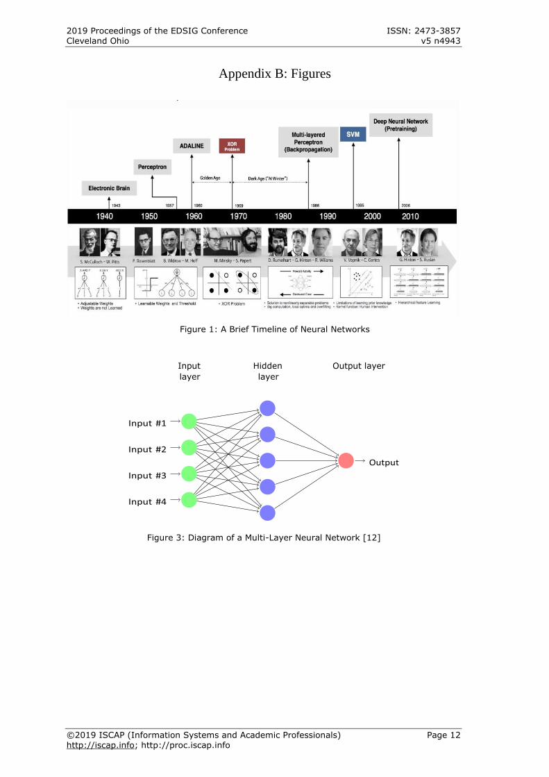
While the idea of neural networks and machine

learning may seem fresh and modern, these

concepts are actually more than seven decades

old. The first neural network dates all the way

back to 1943, when neurophysiologist Warren

McCulloch and mathematician Walter Pitts were

exploring the functions of neurons. During their

research, they published a paper on how they

thought neurons might work and modeled their

ideas into a simple neural network using

electrical circuits [6].

As computer technology made great

advances in the 1950’s, so did neural networks.

In 1959, Bernard Widrow and Marcian Hoff, two

Stanford students, developed the first neural

networks to be successfully applied to a real-

world problem. They called these models

"ADALINE" and "MADALINE". These neural

networks were created to recognize binary

patterns to help predict the next bit in the line

of streaming bits from the phone lines [6]. More

specifically, this technology made it possible to

reduce excess noise over the phone line and is

actually still in use even today [5]! Widrow and

Hoff continued their work well into the 1960’s,

developing new learning procedures that

continued to advance the field of neural network

modeling.

Widrow and Hoff’s innovations were just the

beginning of what was considered the "Golden

Age" of neural network development. Between

the late 1950’s and early 1970’s, many

breakthroughs were made in the field of

computing and neural networks including the

construction of perceptrons with learnable

weights, thresholds and implementation of logic

functions such as AND, OR and NOT. However,

by the end of the 1960’s, researchers begin to

realize that perceptrons could not learn XOR

functions. This issue was exposed in the book

"Preceptrons", written by Marvin Minsky and

Seymor Papert. In this book, Minsky and Papert

not only showed that the preceptron was

incapable of learning a simple XOR function, but

they proved that it was theoretically impossible

for it to learn this function, no matter how long

it trained [7]. Minsky’s findings became known

as the XOR Problem and eventually lead to a

nearly two decade long pause in neural network

research, known as the Dark Age. It was not

until 1986 that neural networks reemerged into

the computing scene with the introduction of

multilayered preceptrons and backpropagation,

both of which are explained in following

sections. This algorithm was what lead to the

start of neural network success with the

creation of the first convolutional neural nets

used to recognize handwritten digits, which is

what much of this paper is centered around [7].

Figure 1: A Brief Timeline of Neural Networks

Appendix B

The goal of this paper is to introduce the reader to the ideas and applications of neural networks through calculus concepts and Python coding. The content is aimed at underclass USMA cadets interested in pursuing additional research in the fields of artificial intelligence and machine

learning. The outline of the sections is as follows: Section 1 discusses the components of a neural network and their functions. Section 2 will cover multi-variable calculus concepts that

are helpful in understanding neural networks such as partial derivatives and gradient descent.

Section 3 will apply the calculus concepts from Section 2 to neural networks through a discussion about the cost function. Section 4 will briefly explain object-oriented programming with classes in Python and how to design a very simple neural network to recognize handwritten digits with these techniques. The final section

will leave the reader with knowledge about what they can do as students to dive deeper into this topic through their studies at USMA and the future that neural network research holds. 2 How do neural networks work?

To understand how neural networks work, it is

necessary to understand the concepts of weight,

bias and threshold. These concepts are applied

through perceptrons, which are the foundation

of many neural networks. A perceptron is an

artificial neuron that takes several binary inputs

to produce a single binary output.

Figure 2: Perceptron Model [11]

Figure 2 shows a perceptron with n number

of binary inputs, x0 to xn, meaning there can be

any number of inputs. This is where the

P w 2 x 2

w n x n

w 1 x 1

w 0 x 0

http://iscap.info/




concepts of weight and threshold come into

play. Weights are applied to the inputs of a

perceptron to represent the importance of each

input. Then, a threshold number is set to

represent what the value must be for the output

to be a 1. If the summation of the inputs

multiplied by the weights is greater than the

threshold, the output is a 1, otherwise it is a 0.

(1)

Putting this into a real-world context:

Imagine that you are trying to decide whether

or not you should take pass to New York City

this weekend. To make your decision, you

consider three things; the weather for the

weekend (x1), how many graded events you

have next week (x2) and whether your

roommate is planning to go with you (x3). Let’s

say the weather is a fairly important factor in

your decision, since you would not really want

to go if it was raining or too cold, so you assign

this input a weight of 3. Assume that your

grades are important to you and you would not

want to risk doing poorly on your WPR’s just to

have a fun weekend, so you assign this a

weight of 5. Assume that you are still willing to

go on pass even if your roommate is not

available because you would still have a good

time by yourself, so you assign this an input

weight of 2. Now, let’s assume that you’re

leaning towards going on pass, so it will not be

too hard to convince yourself to go, so you set

a threshold of 5. After checking the weather,

you see that it is going to rain all weekend, so

you assign x1 an input of 0. You check you AY

Calendar and decide you have a fairly empty

week in terms of graded events, so you assign

x2 to 1. Your roommate also agrees to take

pass with you, so you assign x3 to 1. Using

Equation 1, the output of these decisions is

equal to 7. Since 7 is greater than the

threshold of 5 that you set for yourself, the

output of your hypothetical perceptron will be

1, meaning that you decide to take pass this

weekend.

By applying what seem like complex

concepts to real-life decision-making

processes, it makes these foreign concepts

much easier to understand. While the previous

example illustrated how one preceptron works,

it is also important to understand how

preceptrons interact to create neural networks

capable of making much more complex

decisions. Neural networks are created by

layers of preceptrons with different inputs,

outputs, weights and thresholds. The outputs

of one layer of preceptrons act as the inputs to

the next layer, as shown in Figure 3. Layers of

perceptrons can be created into networks

capable of computing logical functions, and if

set up correctly, they are theoretically capable

of computing any and all logical functions [8].

Figure 3: Diagram of a Multi-Layer Neural Network [12] -Appendix B

While preceptrons are an extremely powerful

tool in creating neural networks, their largest

limitation is that they are only capable of

outputting 0 or 1. This may not seem

problematic in a small-scale setting but imagine

if for every computation in every layer of a

neural network, the outcome just barely

scraped by the threshold. This can lead to a

somewhat questionable output; however, this

output not only effects the decision of that one

preceptron, it also feeds into the inputs of the

next layer of perceptrons, causing an increase

in uncertainty for each output it effects.

Therefore, a small change in the weight of one

perceptron can also lead to a large change in

output. This uncertainty can build up

exponentially and greatly affect the overall

outputs of neural network.

A solution to this limitation was to create the

Sigmoud neuron. Sigmoud neurons are

modeled the exact same way as perceptrons but

are capable of outputting any value from 0 to 1,

for example 0.32. This allows for small changes

in weights that only cause small changes in

outputs, making results much more accurate.

One of the first applications of perceptrons

and Sigmoud neurons came into play with the

convolutional neural networks used to

recognize handwritten digits mentioned in the

introduction. These networks were created to

recognize handwritten digits using data from

the MNIST, a dataset containing over 60,000

training images of digits written by over 250

different people [9]. Each individual digit is

represented by a 28x28 pixel image. Since this

network was trained using individual digits, the

first step in solving this problem is solving the

segmentation problem, which consists of

breaking up a multi-digit number into

individual digits. While the human brain can

easily solve this problem, it is much more

difficult for a computer to interpret.

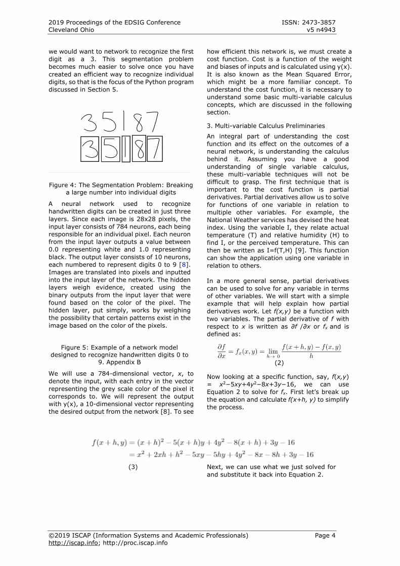
Using Figure 4, we would want the computer

to segment the number 35,187 into its

individual components. Using this, for example,

http://iscap.info/




we would want to network to recognize the first

digit as a 3. This segmentation problem

becomes much easier to solve once you have

created an efficient way to recognize individual

digits, so that is the focus of the Python program

discussed in Section 5.

Figure 4: The Segmentation Problem: Breaking a large number into individual digits

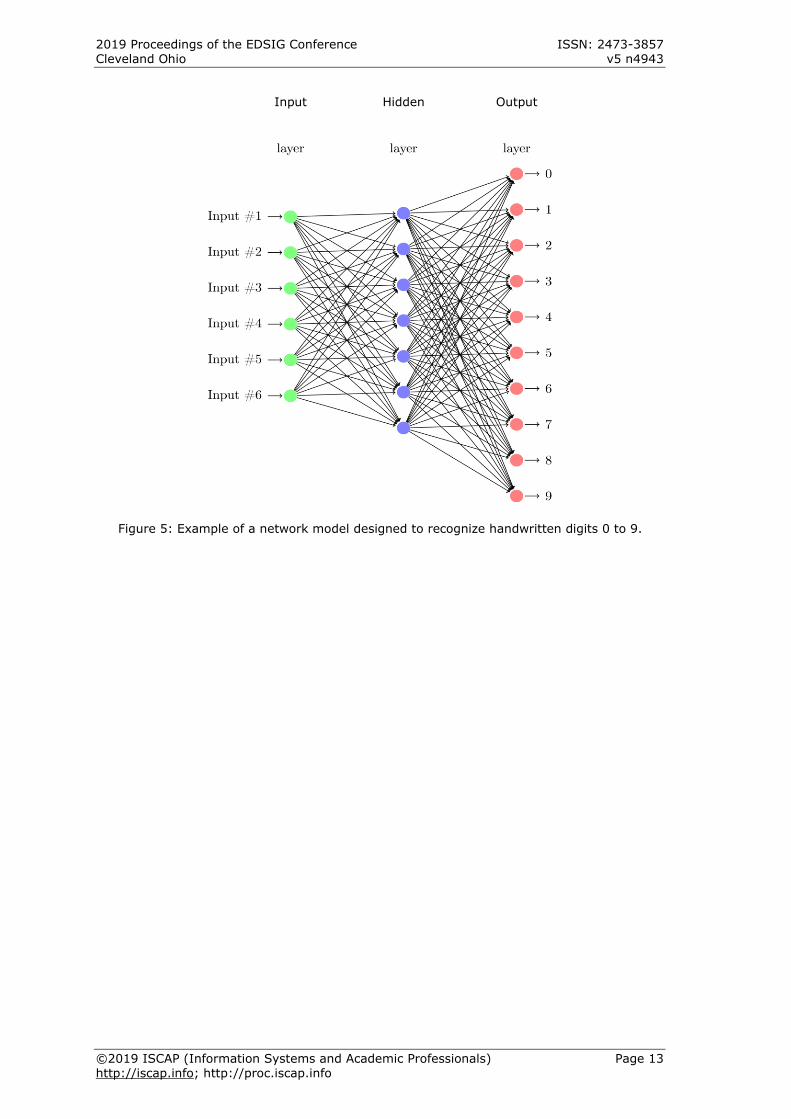
A neural network used to recognize

handwritten digits can be created in just three

layers. Since each image is 28x28 pixels, the

input layer consists of 784 neurons, each being

responsible for an individual pixel. Each neuron

from the input layer outputs a value between

0.0 representing white and 1.0 representing

black. The output layer consists of 10 neurons,

each numbered to represent digits 0 to 9 [8].

Images are translated into pixels and inputted

into the input layer of the network. The hidden

layers weigh evidence, created using the

binary outputs from the input layer that were

found based on the color of the pixel. The

hidden layer, put simply, works by weighing

the possibility that certain patterns exist in the

image based on the color of the pixels.

Figure 5: Example of a network model designed to recognize handwritten digits 0 to

9. Appendix B

We will use a 784-dimensional vector, x, to

denote the input, with each entry in the vector

representing the grey scale color of the pixel it

corresponds to. We will represent the output

with y(x), a 10-dimensional vector representing

the desired output from the network [8]. To see

how efficient this network is, we must create a

cost function. Cost is a function of the weight

and biases of inputs and is calculated using y(x).

It is also known as the Mean Squared Error,

which might be a more familiar concept. To

understand the cost function, it is necessary to

understand some basic multi-variable calculus

concepts, which are discussed in the following

section.

3. Multi-variable Calculus Preliminaries

An integral part of understanding the cost

function and its effect on the outcomes of a

neural network, is understanding the calculus

behind it. Assuming you have a good

understanding of single variable calculus,

these multi-variable techniques will not be

difficult to grasp. The first technique that is

important to the cost function is partial

derivatives. Partial derivatives allow us to solve

for functions of one variable in relation to

multiple other variables. For example, the

National Weather services has devised the heat

index. Using the variable I, they relate actual

temperature (T) and relative humidity (H) to

find I, or the perceived temperature. This can

then be written as I=f(T,H) [9]. This function

can show the application using one variable in

relation to others.

In a more general sense, partial derivatives

can be used to solve for any variable in terms

of other variables. We will start with a simple

example that will help explain how partial

derivatives work. Let f(x,y) be a function with

two variables. The partial derivative of f with

respect to x is written as ∂f /∂x or fx and is

defined as:

(2)

Now looking at a specific function, say, f(x,y)

= x2−5xy+4y2−8x+3y−16, we can use

Equation 2 to solve for fx. First let’s break up

the equation and calculate f(x+h, y) to simplify

the process.

(3)

Next, we can use what we just solved for

and substitute it back into Equation 2.

http://iscap.info/




(4)

Now that we have solved for the partial

derivative of this function, we can interrupt it.

In this case, fx(x,y) would represent how the

entirety of the function changes as x changes

while holding y constant. To better understand

this concept, it is easy to visualize how a partial

derivative works using a three-dimensional

graph. If f(x,y) above were graphed and sliced

with a plane representing a constant y-value,

measuring the slope of the resulting curve

would give you fx(x,y) at that specific y-value

[10].

Partial derivatives represent a rate of change of

a function with respect to a single variable,

however there are many possible directions of

travel in a multi-dimensional function. Assume

you want to find the direction of travel that will

increase f most rapidly. This is called the

gradient which could also be considered the full

derivative since this is the idea that gradient

represents.

The gradient of a function, f, is represented by

a vector composed of partial derivatives and is

denoted as ▽f. A gradient with a 2-dimensional

input will produce a 2-dimensional output as

seen in Equation 4, which is represented by a

vector field [10]. This logic also holds true for

a function of any dimension, but to keep things

relatively simple we focus on 2-dimensional

functions for most of this section. For example,

imagine we have the function f(x,y) = x2− xy.

(5)

Now that we understand how to compute these

vector fields, we can focus more on

interpreting them. Going back to the case

where the input of f is two-dimensional,

imagine you have a generic input point (x0,y0).

Computing the gradient will turn each of the

input points into the vector,

(6)

This vector will indicate the behavior of the

function around the point (x0,y0). This concept

is relatively easy to understand if you relate it

back to something familiar, say land

navigation. Think of the graph of f as

mountainous terrain like the summer land

navigation course. Now imagine you are

standing on Bull Hill and you want to find the

fastest way to your point (x0,y0), which is

directly above you. The slope of the terrain will

determine the direction you walk. If you step

straight in the positive x-direction, the slope is

.

if you step straight in the positive y-direction

the slope is . But if you walk any other

direction it will be a combination of those two

slopes. By solving for the gradient at your

current position, you can find the direction of

steepest ascent. So, if you walk in the direction

of the gradient, you will be walking straight up

Bull Hill directly towards your point. Now if you

find the magnitude of the gradient, you will

know what the actual slope is in that direction

[10].

Once you move past two-dimensional functions, this concept is not easily visualized

in the same way, however the concept remains the same no matter how many dimensions a function is. The gradient vector of a function

http://iscap.info/




will always give you the direction of fastest

increase. Tying this back to neural networks, the concept of gradient is used when computing the cost function for a network to

determine the efficiency of the model. 4. The cost function

The goal of the neural network in Section 5 is to

predict handwritten digits as accurately as

possible. Predictions of the neural network

pictured in Figure 5 are outputted in the form of

a 10-dimensional transpose vector. For

example, if an input image, x, depicts a

handwritten 7, the desired output vector would

be y(x) = (0,0,0,0,0,0,0,1,0,0)T. To quantify

how well our model works, we can create a cost

function. Assuming you are somewhat familiar

with statistics, the cost function of a neural

network works similarly to the regression

function of a statistical model. The closer the

cost function is to 0, the more accurately it is

interpreting its input values.

Ultimately, the goal of the neural network is to

create an algorithm that determines the weights

and biases necessary to minimize cost and

approximate y(x) for all training inputs x [8].

This is quantified using a cost function, which is

generally defined as,

(7)

where w denotes the collection of all weights in

the network, b denotes all the biases, n the total

number of training inputs, and a the vector of

outputs from the network when x is the input.

C(w,b) becomes smaller the closer y(x) is to a

for all training inputs x. When y(x) is not close

to a for a large number of training inputs,

C(w,b) becomes large [8].

Referencing the previous section on multi-

variable calculus techniques, to minimize the

cost function, we will apply the concept of

gradient descent. Ultimately, the goal is to

minimize cost. For the sake of simplification,

we can ignore most of the complicated aspects

of neural network connections and how the

cost function is derived in order to focus on the

concept itself, so we can just imagine that we

have been given a function with many

variables and that we want to minimize it.

Say we have been given the function C(v)

where v = v1,v2,... so v represents a

combination of many variables. We want to use

gradient descent to find where C(v) reaches its

global minimum [8]. Now instead of thinking of

this function as a mountain like we did in the

previous section, we will think of it more as a

valley and we are looking for the quickest way

to the deepest point. To simulate this, you can

think of a ball rolling down into this valley,

since it will eventually reach the lowest point if

allowed to roll freely with no physical

constraints [8]. We can model the movement

of the "ball" in relation to the function C(v)

using the function,

(8)

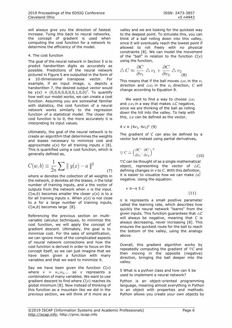
This means that if the ball moves △v1 in the v1

direction and △v2 in the v2 direction, C will

change according to Equation 8.

We want to find a way to choose △v1

and △v2 in a way that makes △C negative,

since we are thinking of the ball as rolling

down the hill into the valley. To help with

this, △v can be defined as the vector,

4 v ≡ (4v1, 4v2)2 (9)

The gradient of C can also be defined by a

vector but instead using partial derivatives,

(10)

▽C can be thought of as a single mathematical

object, representing the vector of △C,

defining changes in v to C. With this definition,

it is easier to visualize how we can make △C

negative. Using the equation:

v ≡−η 5 C

(11)

η is represents a small positive parameter

called the learning rate, which describes how

quickly the neural network "learns" from the

given inputs. This function guarantees that △C

will always be negative, meaning that C is

always decreasing, never increasing [8]. This

ensures the quickest route for the ball to reach

the bottom of the valley, using the analogy

above.

Overall, this gradient algorithm works by repeatedly computing the gradient of ▽C and

then moving in the opposite (negative) direction, bringing the ball deeper into the valley.

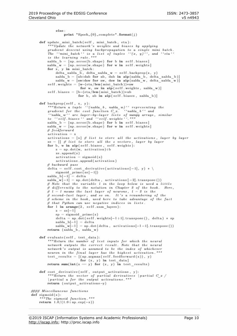
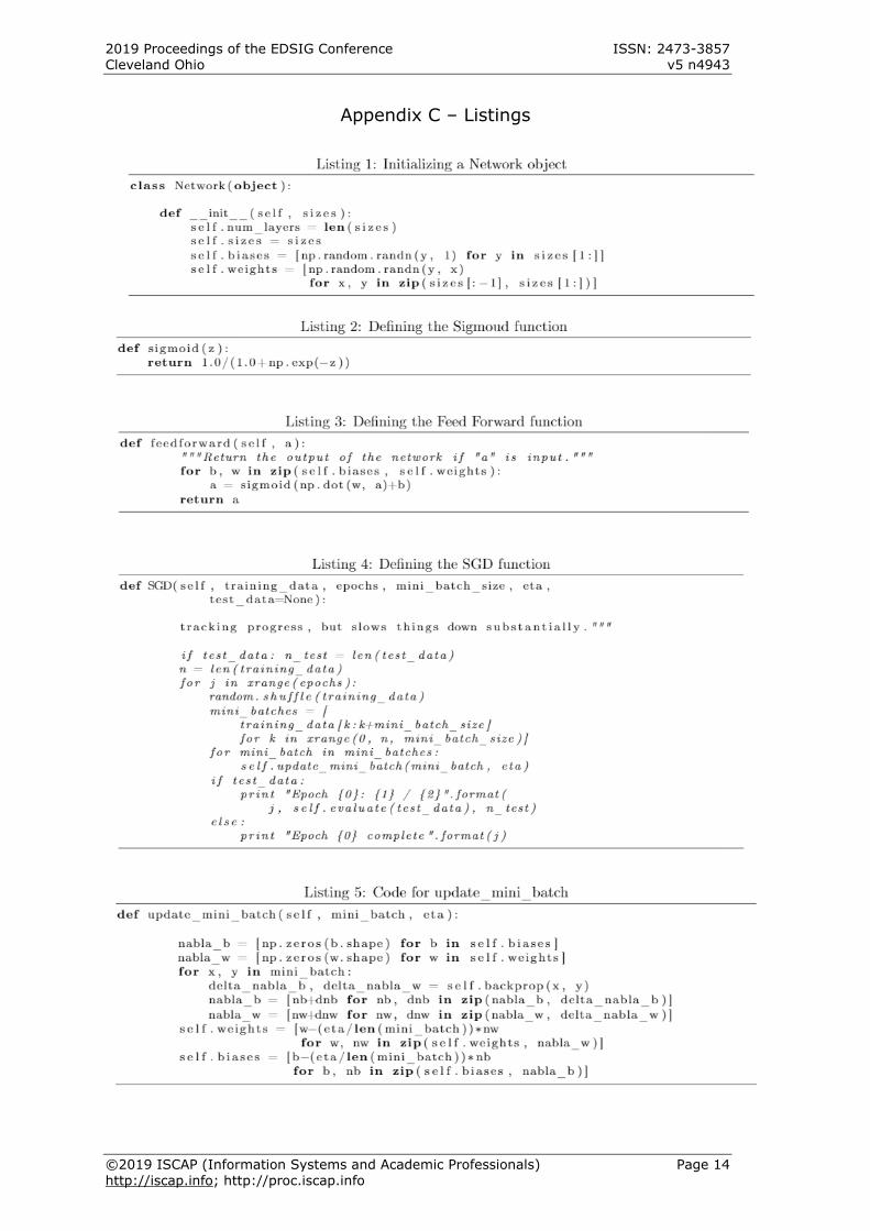
5 What is a python class and how can it be

used to implement a neural network?

Python is an object-oriented programming

language, meaning almost everything in Python

is an object with properties and methods.

Python allows you create your own objects by

http://iscap.info/




creating a Class. Classes work similarly to

blueprints, allowing you to construct and

customize your own objects [13]. To create a

Class, you must first define it and then initialize

your object using the built-in __init__()

function. This function assigns values to the

object properties that you create [13]. For our

neural network, we will create a class called

Network to work with. When Network is

initialized, it will be assigned a value called

"size" which will help to define the number of

layers (num_layers), the weights and the

biases. It will also contain the parameter self

which is essentially just a reference to the

current instance of the class and is used to

access variables that belong to a class [13].

Listing 1 (Appendix C)

In this code, sizes contains the number of

neurons in the respective layers. For example,

if you want to create a Network object with 4

neurons in the first layer, 5 neurons in the

second layer and 1 neuron in the final layer,

similarly to Figure 3, you would use the code

[8]:

net = Network([4, 5, 1])

Weights and biases in the Network object are

initialized randomly using the Numpy

np.random.randn function. These weights and

biases are stored as lists of Numpy matrices [8].

Objects in Python can also contain methods that

you create. Methods are functions that

specifically belong to that object [13]. We can

use methods to define important parts and

functions of our network. For example, we can

start by defining a Sigmoud neuron which

contains the sigmoud function. In this

definition, z is a vector.


Next, we can define a feedforward method,

which, when given an input a for the network

returns the corresponding output by applying

the equation, aI = σ(wa + b). In this equation,

a is the vector of activations of the second layer

of neurons, w is a matrix of the weights, b is a

vector of the biases and σ is the sigmoud

function [12].


The main goal of the Network object is to learn.

To do this, we can define a stochastic gradient

descent, or SGD function. This function takes a

few different inputs. The training data is a list of

tuples (x, y) that represent the training inputs

from the MNIST data and the corresponding

desired output. The variables epoch and

mini_batch_size are the number of epochs to

train for and the size of the mini-batches to use

when sampling. eta is the learning rate and

test_data is an optional argument that will

allow the user to track the learning progress by

printing out partial progress after each epoch of

training [8].


In each epoch, the code starts by randomly

shuffling the training data and partitioning it

into mini-batches of the specified size. For each

mini_batch, a single step of gradient descent is

applied with the code

self.update_mini_batch(mini_batch, eta).

Using the training data in mini_batch this

updates the network weights and biases

according to a single iteration of gradient

descent [8]. The code for

update_mini_batch is as follows:


The most important line of this function is:

delta_nabla_b, delta_nabla_w =

self.backprop(x, y)

This part of the function does most of the work by invoking the back-propagation algorithm, which was briefly described in a previous section. This is basically just a quick way of computing the gradient cost function [8].

Overall, the way this whole function works is by computing the gradients for every training example in mini_batch and then updating self’s weights and biases appropriately. Ultimately, these are the most important parts of the program, but all the code can be seen in Appendix A, which will show how some functions

are working behind the scenes.

6 What’s next?

Today, neural networks are being used to

create groundbreaking discoveries across

many different fields. Researchers have

recently created a neural network that can

detect congestive heart failure by analyzing

just one single heartbeat. This is just one

example of the incredible work that this

technology is being used for.

Every day, researchers are working towards

neural network models to close the gap

http://iscap.info/




between the human brain and artificial

intelligence. As they make discoveries, they

get closer to creating learning algorithms that

more closely resemble the human brain. Right

now, researchers are even working on creating

optical neural networks that will come up with

their own training examples through

observation, much like human learn through

observation from a very young age.

Neural networks and deep learning are the key

to future technology and innovation. The closer

we can resemble them human learning

processes, the better we can implement

artificial intelligence to model human behavior.

Not only would this be an incredible stride for

STEM fields, but also for psychology and human

studies alike, who still struggle to understand

exactly how the brain works to make decisions

and converts learning to behavior.

REFERENCES

[1] Mittal, Vartul. “Top 15 Deep Learning

Applications That Will Rule the World in 2018 and Beyond.” Medium, Medium, 9 Oct. 2017, medium.com/breathe-publication/top-15-deep-learning-applications-that-will-rule-the-world-in-2018-and-beyond-7c6130c43b01.

[2] Trafton, Anne, and MIT News Office. “The

Future of Agriculture Is Computerized.” MIT News, MIT, 3 Apr. 2019, news.mit.edu/2019/algorithm-growing-agriculture-0403.

[3] Lynch, Matthew. “How Machine Learning Is Helping Us to Understand the Brain.” The Tech Edvocate, 19 Apr. 2019,

www.thetechedvocate.org/how-machine-learning-is-helping-us-to-understand-the-brain/.

[4] “Neural Networks - What Are They and Why Do They Matter?” SAS, www.sas.com/en_us/insights/analytics/neural-networks.html.

[5] Jiaconda. “A Concise History of Neural

Networks.” Medium, Towards Data Science, 8 Apr. 2019, towardsdatascience.com/a-concise-history-of-neural-networks-

2070655d3fec.

[6] Pang, Jimmy, and Caroline Clabaugh. “Neural Networks.” Neural Networks - Sophomore College 2000, cs.stanford.edu/people/eroberts/courses/soco/projects/neural-networks/index.html.

[7] Beam, Andrew. “Deep Learning 101- Part I: History and Background, Machine Learning

and Medicine.” Deep Learning 101 - Part 1: History and Background, beamandrew.github.io/deeplearning/2017/

02/23/deep_learning_101_part1.html.

[8] Nielsen, Michael A. “Neural Networks and Deep Learning.” Neural Networks and Deep Learning, Determination Press, 1 Jan. 1970,

neuralnetworksanddeeplearning.com/chap1.html.

[9] “Partial Derivatives.” Calculus: Early Transcendentals, by James Stewart, 8th ed., Cengage Learning, 2016, pp. 914–919.

[10] “Multivariable Calculus.” Khan Academy, Khan Academy,

www.khanacademy.org/math/multivariable-calculus.

[11] m0nhawk. “Diagram of a Perceptron.” Stack Exchange, tex.stackexchange.com/ questions/104334/tikz-diagram-of-a-perceptron.

[12] Fauske, Kjell. “TikZ and PGF Examples.” TeXample.net,

www.texample.net/tikz/examples/ neural-network/.

[13] “Python Classes and Objects.” W3Schools, www.w3schools.com/python/python_ classes.asp.

http://iscap.info/




Appendix A: Complete Coding Example with Comments

http://iscap.info/




http://iscap.info/




http://iscap.info/




Appendix B: Figures

Figure 1: A Brief Timeline of Neural Networks

Input

layer

Hidden

layer

Output layer

Figure 3: Diagram of a Multi-Layer Neural Network [12]

http://iscap.info/




Input Hidden Output

Figure 5: Example of a network model designed to recognize handwritten digits 0 to 9.

http://iscap.info/




Appendix C – Listings

http://iscap.info/

Documents

A Neural Networks Primer for USMA Cadetsproc.iscap.info/2019/pdf/4943.pdf · A Neural Networks Primer for USMA Cadets Elie Alhajjar [email protected] Taylor Bradley United