A nearest neighbor bootstrap for resampling hydrologic …civil.colorado.edu/~balajir/Adv-Data-material/CVEN-6833/papers-2... · WATER RESOURCES RESEARCH, VOL. 32, NO. 3, PAGES 679-693,

WATER RESOURCES RESEARCH, VOL. 32, NO. 3, PAGES 679-693, MARCH 1996

A nearest neighbor bootstrap for resampling hydrologic timeseriesUpmanu Lall and Ashish SharmaUtah Water Research Laboratory, Utah State University, Logan

Abstract. A nonparametric method for resampling scalar or vector-valued time series isintroduced. Multivariate nearest neighbor probability density estimation provides the basisfor the resampling scheme developed. The motivation for this work comes from a desireto preserve the dependence structure of the time series while bootstrapping (resampling itwith replacement). The method is data driven and is preferred where the investigator isuncomfortable with prior assumptions as to the form (e.g., linear or nonlinear) ofdependence and the form of the probability density function (e.g., Gaussian). Such priorassumptions are often made in an ad hoc manner for analyzing hydrologic data.Connections of the nearest neighbor bootstrap to Markov processes as well as its utility ina general Monte Carlo setting are discussed. Applications to resampling monthlystreamflow and some synthetic data are presented. The method is shown to be effectivewith time series generated by linear and nonlinear autoregressive models. The utility ofthe method for resampling monthly streamflow sequences with asymmetric and bimodalmarginal probability densities is also demonstrated.

Introduction

Autoregressive moving average (ARMA) models for timeseries analysis are often used by hydrologists to generate syn-thetic streamflow and weather sequences to aid in the analysisof reservoir and drought management. Hydrologic time seriescan exhibit the following behaviors, which can be a problem forcommonly used linear ARMA models: (1) asymmetric and/ormultimodal conditional and marginal probability distributions;(2) persistent large amplitude variations at irregular time in-tervals; (3) amplitude-frequency dependence (e.g., the ampli-tude of the oscillations increases as the oscillation period in-creases); (4) apparent long memory (this could be related to(2) and/or (3)); (5) nonlinear dependence between xt versusxt_T for some lag r; and (6) time irreversibility (i.e., the timeseries plotted in reverse time is "different" from the time seriesin forward time). The physics of most geophysical processes istime irreversible. Streamflow hydrographs often rise rapidlyand attenuate slowly, leading to time irreversibility.

Kendall and Dracup [1991] have argued for simple resam-pling schemes, such as the index sequential method, forstreamflow simulation in place of ARMA models, suggestingthat the ARMA streamflow sequences usually do not "look"like real streamflow sequences. An alternative is presented inthe work of Yakowitz [Yakowitz, 1973, 1979; Schuster and Ya-kowitz, 1979; Yakowitz, 1985, 1993; Karlsson and Yakowitz,1987a, b], Smith et al [1992], Smith [1991], and Tarboton et al.[1993] who consider the time series as the outcome of aMarkov process and estimate the requisite probability densitiesusing nonparametric methods. A resampling technique orbootstrap for scalar or vector-valued, stationary, ergodic timeseries data that recognizes the serial dependence structure ofthe time series is presented here. The technique is nonpara-

Copyright 1996 by the American Geophysical Union.

Paper number 95WR02966.0043-1397/96/95WR-02966$05.00

metric; that is, no prior assumptions as to the distributionalform of the underlying stochastic process are made.

The bootstrap [Efron, 1979; Efroh and Tibishirani, 1993] is atechnique that prescribes a data resampling strategy using therandom mechanism that generated the data. Its applicationsfor estimating confidence intervals and parameter uncertaintyare well known [see Hardle and Bowman, 1988; Tasker, 1987;Woo, 1989; Zucchini and Adamson, 1989]. Usually the boot-strap resamples with replacement from the empirical distribu-tion function of independent, identically distributed data. Thecontribution of this paper is the development of a bootstrap fordependent data that preserves the dependence in a probabi-listic sense. This method should be useful for the Monte Carloanalysis of a variety of hydrologic design and operation prob-lems where time series data on one or more interacting vari-ables are available.

The underlying concept of the methodology is introducedthrough Figure 1. Consider that the serial dependence is lim-ited to the two previous lags; that is, xt depends on the twoprior values xt_l and xt_2. Denote this ordered pair, orbituple, at a time tt by D,. Let the corresponding succeedingvalue be denoted by S. Consider the k nearest neighbors of D,as the k bituples in the time series that are closest in terms ofEuclidean distance to D,. The first three nearest neighbors aremarked as D1? D2, and D3. The expected value of the forecastS can be estimated as an appropriate weighted average of thesuccessors xt (marked as 1,2, and 3, respectively) to these threenearest neighbors. The weights may depend inversely on thedistance between D, and its k nearest neighbors D1? D2, • • • ,D^. A conditional probability density f(x\Df) may be evaluatedempirically using a nearest neighbor density estimator [seeSilverman, 1986, p. 96] with the successors xl9 ••• , xk. Forsimulation the xi can be drawn randomly from one of the ksuccessors to the D1? D2, • • • , D^ using this estimated condi-tional density. Here, this operation will be done by resamplingthe original data with replacement. Hence the procedure de-veloped is termed a nearest neighbor time series bootstrap. In

679

680 LALL AND SHARMA: NEAREST NEIGHBOR BOOTSTRAP

I I S S

f i l j | f i l j| Values of' : ' ' s ^ > '

time

Figure 1. A time series from the model xf + 1 = (1 - 4(xt -0.5)2). This is a deterministic, nonlinear model with a timeseries that looks random. A forecast of the successor to thebituple D;, marked as S in the figure, is of interest. The "pat-terns" or bituples of interest are the filled circles, near thethree nearest neighbors D1} D2, and D3 to the pattern Dz. Thesuccessors to these bituples are marked as 1, 2, and 3, respec-tively. Note how the successor (1) to the closest nearest neigh-bor (DJL) is closest to the successor (S) of D,. A sense of themarginal probability distribution of xf is obtained by looking atthe values of xt shown on the right side of the figure. As thesample size n increases, the sample space of x gets filled inbetween 0 and 1, such that the sample values are arbitrarilyclose to each other, but no value is ever repeated exactly.

summary, one finds k patterns in the data that are "similar" tothe current pattern and then operates on their respective suc-cessors to define a local regression, conditional density, orresampling.

The nearest neighbor probability density estimator and itsuse with Markov processes is reviewed in the next section. Theresampling algorithm is described after that. Applications tosynthetic and streamflow data are then presented.

BackgroundIt is natural to pursue nonparametric estimation of proba-

bility densities and regression functions through weighted localaverages of the target function. This is the foundation fornearest neighbor methods. The recognition of the nonlinearityof the underlying dynamics of geophysical processes, gains incomputational ability, and the availability of large data setshave spurred the growth of the nonparametric literature. Thereader is referred to work by Silverman [1986], Eubank [1988],Hiirdle [1989, 1990], and Scott [1992] for accessible mono-graphs. Gyorfi et al. [1989] provide a theoretical account that isrelevant for time series analysis. Lall [1995] surveys hydrologicapplications. For time series analysis a moving block bootstrap(MBB) was presented by Kunsch [1989]. Here a block of mobservations is resampled with replacement, as opposed to asingle observation in the bootstrap. Serial dependance is pre-served within, but not across, a block. The block length mdetermines the order of the serial dependence that can bepreserved. Objective procedures for the selection of the blocklength m are evolving. Strategies for conditioning the MBB onother processes (e.g., runoff on rainfall) are not obvious. Ourinvestigations indicated that the MBB may not be able to

reproduce the sample statistics as well as nearest neighborbootstrap presented here.

The k nearest neighbor (A>nn) density estimator is definedas [Silverman, 1986, p. 96]

/NN(X) =kin kin

(1)

where k is the number of nearest neighbors considered, d is thedimension of the space, cd is the volume of a unit sphere in ddimensions (cl = 2, c2 = TT, c3 = 47T/3, • • • , cd =[7rd/2/Y(d/2 + 1)]), rk(x) is the Euclidean distance to theA:th-nearest data point, and Vk(\) is the volume of a d-dimensional sphere of radius rk(\).

This estimator is readily understood by observing that for asample of size n, we expect approximately {nf(x)Vk(x)} ob-servations to lie in the volume Vk(x). Equating this to thenumber observed, that is, k, completes the definition.

A generalized nearest neighbor density estimator [Silver-man, 1986, p. 97], defined in (2), can improve the tail behaviorof the nearest neighbor density estimator by using a monoton-ically and possibly rapidly decreasing smooth kernel function.

7GNN(X) =1

rt(x)nx — x/rk(x) (2)

The "smoothing" parameter is the number of neighborsused, k, and the tail behavior is determined by the kernel K(i).The kernel has the role of a weight function (data vectors X,closer to the point of estimate x are weighted more), and canbe chosen to be any valid probability density function. Asymp-totically, under optimal mean square error (MSE) arguments,k should be chosen proportional to ^4/(^+4) for a probabilitydensity that is twice differentiable. However, given a singlesample from an unknown density, such a rule is of little prac-tical utility. The sensitivity to the choice of A: is somewhat loweras a kernel that is monotonically decreasing with rk(x) is used.A new kernel function that weights the j'th neighbor of x, usinga kernel that depends on the distance between x, and its ythneighbor is developed in the resampling methodology section.

Yakowitz (references cited earlier) developed a theoreticalbasis for using nearest neighbor and kernel methods for timeseries forecasting and applied them in a hydrologic context. Inthose papers Yakowitz considers a finite order, continuousparameter Markov chain as an appropriate model for hydro-logic time series. He observes that discretization of the statespace can quickly lead to either an unmanageable number ofparameters (the curse of dimensionality) or poor approxima-tion of the transition functions, while the ARMA approxima-tions to such a process call for restrictive distributional andstructural assumptions. Strategies for the simulation of dailyflow sequences, one-step-ahead prediction, and the conditionalprobability of flooding (flow crossing a threshold) are exem-plified with river flows and shown to be superior to ARMAmodels. Seasonality is accommodated by including the calen-dar date as one of the predictors. Yakowitz claims that thiscontinuous parameter Markov chain approach is capable ofreproducing any possible Hurst coefficient. Classical ARMAmodels are optimal only under squared error loss and only forlinear operations on the observables. The loss/risk functionsassociated with hydrologic decisions (e.g., whether to declare aflood warning or not) are usually asymmetric. The nonpara-metric framework allows attention to be focused directly on

LALL AND SHARMA: NEAREST NEIGHBOR BOOTSTRAP 681

calculating these loss functions and evaluating the conse-quences.

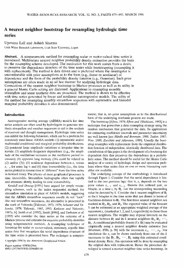
The example of Figure 1 is now extended to show how thenearest neighbor method is used in the Markov framework.One step Markov transition functions are considered. Therelationship between xt+l and xt is shown in Figure 2. Thecorrelation between xt and xt+l is 0, even though there isclear-cut dependence between the two variables.

Consider an approximation of the model in Figure 1 by amultistate, first-order Markov chain, where transitions from,say, state 1 for xt (0 to 0.25 in Figure 2) to states 1, 2, 3, or 4for xt+l are of interest. The state / to state; transition prob-ability ptj is evaluated by counting the relative fraction oftransitions from state i to state j. The estimated transitionprobabilities depend on the number of states chosen as well astheir actual demarcation (e.g., one may need a nonuniformgrid that recognizes variations in data density). For the non-linear model used in our example, a fine discretization wouldbe needed. Given a finite data set, estimates of the multistatetransition probabilities may be unreliable. Clearly, this situa-tion is exacerbated if one considers higher dimensions for thepredictor space. Further, a reviewer has observed that a dis-cretization of a continuous space Markov process is not nec-essarily Markov.

Now consider the nearest neighbor approach. Consider twoconditioning points x*A and x*B. The k nearest neighbors ofthese points are in the dashed windows^ and B, respectively.The neighborhoods are seen to adapt to variations in the sam-pling density of*,. Since such neighborhoods represent movingwindows (as opposed to fixed windows for the multistateMarkov chain) at each point of estimate, we can expect re-duced bias in the recovery of the target transition functions.The one step transition probabilities at x* can be obtainedthrough an application of the nearest neighbor density estima-tor to the xt + l values that fall in windows like A and B. Aconditional bootstrap of the data can be obtained by resam-pling from this set of xt+l values. Since each transition prob-ability estimate is based on k points, the problem faced in amultistate Markov chain model of sometimes not having anadequate number of events or state transitions to develop anestimate is circumvented.

The Nearest Neighbor Resampling AlgorithmIn this section a new algorithm for generating synthetic time

series samples by bootstrapping (i.e., resampling the originaltime series with replacement) is presented. Denote the timeseries byxt,t=l, — - , n, and assume a known dependencestructure, that is, which and how many lags the future flow willdepend on. This conditioning set is termed a "feature vector,"and the simulated or forecasted value, the "successor." Thestrategy is to find the historical nearest neighbors of the cur-rent feature vector and resample from their successors. Ratherthan resampling uniformly from the k successors, a discreteresampling kernel is introduced to weight the resamples toreflect the similarity of the neighbor to the conditioning point.This kernel decreases monotonically with distance and adaptsto the local sampling density, to the dimension of the featurevector, and to boundaries of the sample space. An attractiveprobabilistic interpretation of this kernel consistent with thenearest neighbor density estimator is also offered. The resam-pling strategy is presented through the following flowchart:

State1 2 3

0.75.

0.5-

0.25.

State4

0 0.25 0.5 0.75 1

Figure 2. A plot of xt+l versus xt for the time series gener-ated from the model xt + l = (1 - 4(xt - 0.5)2). The statespace for x is discretized into four states, as shown. Also shownare windows^ and B with "whiskers" located over two pointsx*A and x*B. These windows represent a k nearest neighbor-hood of the corresponding xt. In general, these windows willnot be symmetric about the xt of interest. One can think ofstate transition probabilities using these windows in much thesame way as with the multistate Markov chain. A value of xt + 1conditional to point A or B can be bootstrapped by appropri-ately sampling with replacement one of the values of xt + l thatfall in the corresponding window.

1. Define the composition of the "feature vector" Dt ofdimension d, e.g.,

Case 1 D,: (*,_!, Jt,_2); d = 2

Case 2

= Ml+M2

Case 3 D,:(*l,_Tl, l,_Mlrl; x2t, *2,_T , *2,_M2T2);

d = Ml + M2 + 1

where rl (e.g., 1 month) and r2 (e.g., 12 months) are lagintervals, and Ml, M2 > 0 are the number of such lagsconsidered in the model.

Case 1 represents dependence on two prior values. Case 2permits direct dependence on multiple time scales, allowingone to incorporate monthly and interannual dependence. Forcase 3, xl and x2 may refer to rainfall and runoff or to twodifferent streamflow stations.

2. Denote the current feature vector as D, and determineits k nearest neighbors among the D,, using the weightedEuclidean distance

1/2

(3)

where vtj is the; th component of Dr, and Wj are scaling weights(e.g., 1 or 1/Sj, where s}- is some measure of scale such as thestandard deviation or range of Vj).

The weights Wj may be specified a priori, as indicated above,or may be chosen to provide the best forecast for a particularsuccessor in a least squares sense [see Yakowitz and Karlsson,1987].

Denote the ordered set of nearest neighbor indices by Jt ^.An element y (/) of this set records the time t associated withthejth closest Dr to D,. Denotejcy(/) as the successor to Dy(/).


0.4

0.0

0.3 -

0.2-

..••'

It

U ; \r•»•"* '•«...*—•"" »

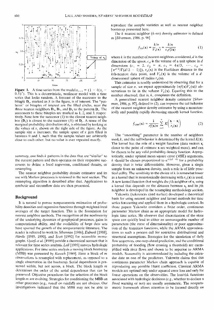
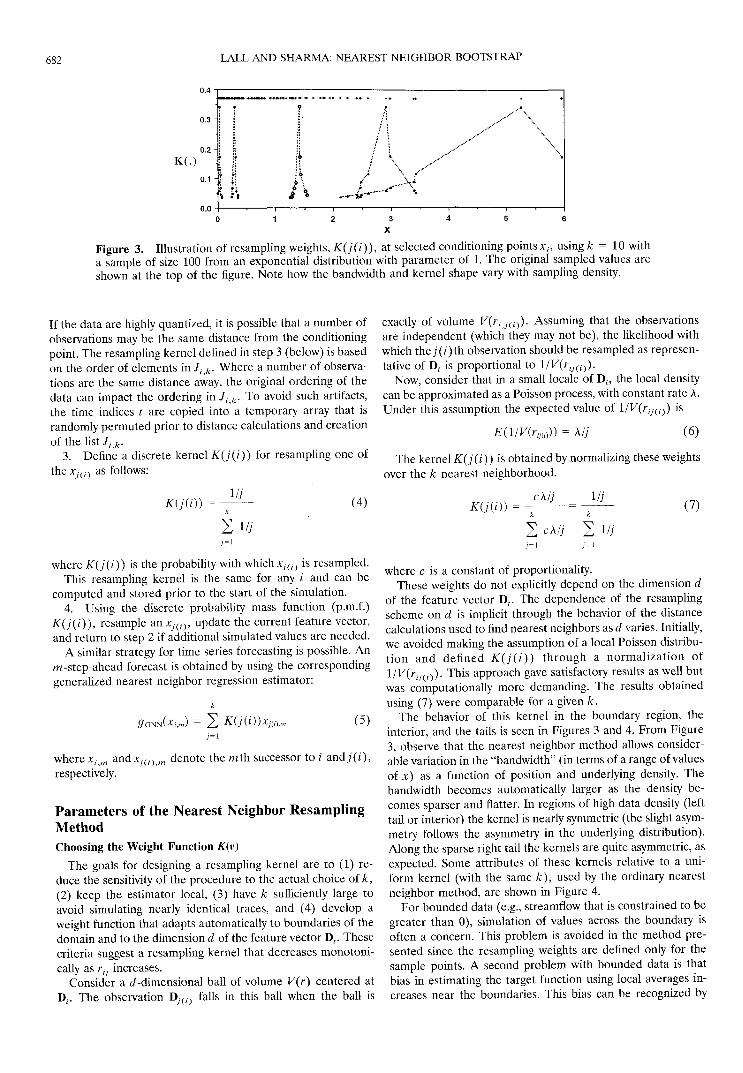
Figure 3. Illustration of resampling weights, K ( j ( i ) ) , at selected conditioning points*,, using k = 10 witha sample of size 100 from an exponential distribution with parameter of 1. The original sampled values areshown at the top of the figure. Note how the bandwidth and kernel shape vary with sampling density.

If the data are highly quantized, it is possible that a number ofobservations may be the same distance from the conditioningpoint. The resampling kernel defined in step 3 (below) is basedon the order of elements in J^k. Where a number of observa-tions are the same distance away, the original ordering of thedata can impact the ordering in J^k. To avoid such artifacts,the time indices t are copied into a temporary array that israndomly permuted prior to distance calculations and creationof the list ]ik.

3. Define a discrete kernel K ( j ( i ) ) for resampling one ofthe jcy-(/) as follows:

(4)

exactly of volume F(r/J(/)). Assuming that the observationsare independent (which they may not be), the likelihood withwhich the j(0tn observation should be resampled as represen-tative of D; is proportional to HV(rij(i}).

Now, consider that in a small locale of D,, the local densitycan be approximated as a Poisson process, with constant rate A.Under this assumption the expected value of llV(rij(i}) is

E ( l l V ( r i j ( l } } } = A/; (6)

The kernel K ( j ( i ) ) is obtained by normalizing these weightsover the k nearest neighborhood.

cXlj 1/7(7)

where K ( j ( i ) ) is the probability with which xj(i} is resampled.This resampling kernel is the same for any / and can be

computed and stored prior to the start of the simulation.4. Using the discrete probability mass function (p.m.f.)

K ( j ( i ) ) , resample an jcy(O, update the current feature vector,and return to step 2 if additional simulated values are needed.

A similar strategy for time series forecasting is possible. Anm -step-ahead forecast is obtained by using the correspondinggeneralized nearest neighbor regression estimator:

(5)

where*, m andzy(/) m denote the rath successor to i and;(0»respectively.

Parameters of the Nearest Neighbor ResamplingMethodChoosing the Weight Function K(v)

The goals for designing a resampling kernel are to (1) re-duce the sensitivity of the procedure to the actual choice of k,(2) keep the estimator local, (3) have k sufficiently large toavoid simulating nearly identical traces, and (4) develop aweight function that adapts automatically to boundaries of thedomain and to the dimension d of the feature vector D,. Thesecriteria suggest a resampling kernel that decreases monotoni-cally as rtj increases.

Consider a d-dimensional ball of volume V(r) centered atD,.. The observation D;(0 falls in this ball when the ball is

where c is a constant of proportionality.These weights do not explicitly depend on the dimension d

of the feature vector D,. The dependence of the resamplingscheme on d is implicit through the behavior of the distancecalculations used to find nearest neighbors as d varies. Initially,we avoided making the assumption of a local Poisson distribu-tion and defined K ( j ( i ) ) through a normalization ofl/K(r,7(0). This approach gave satisfactory results as well butwas computationally more demanding. The results obtainedusing (7) were comparable for a given k.

The behavior of this kernel in the boundary region, theinterior, and the tails is seen in Figures 3 and 4. From Figure3, observe that the nearest neighbor method allows consider-able variation in the "bandwidth" (in terms of a range of valuesof jc) as a function of position and underlying density. Thebandwidth becomes automatically larger as the density be-comes sparser and flatter. In regions of high data density (lefttail or interior) the kernel is nearly symmetric (the slight asym-metry follows the asymmetry in the underlying distribution).Along the sparse right tail the kernels are quite asymmetric, asexpected. Some attributes of these kernels relative to a uni-form kernel (with the same k), used by the ordinary nearestneighbor method, are shown in Figure 4.

For bounded data (e.g., streamflow that is constrained to begreater than 0), simulation of values across the boundary isoften a concern. This problem is avoided in the method pre-sented since the resampling weights are defined only for thesample points. A second problem with bounded data is thatbias in estimating the target function using local averages in-creases near the boundaries. This bias can be recognized by


0.4

0.3-

0.2-

0.1 -

0.0

Centroid of K(j(i))

Uniform Kerne]yCentroid

£/

0.00 0.02 0.04 0.06 0.08 0.22 0.26 0.30 0.34

(a)

X

(b)

K() 0.2-

2.0 6.0

(c)

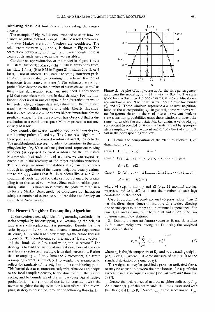
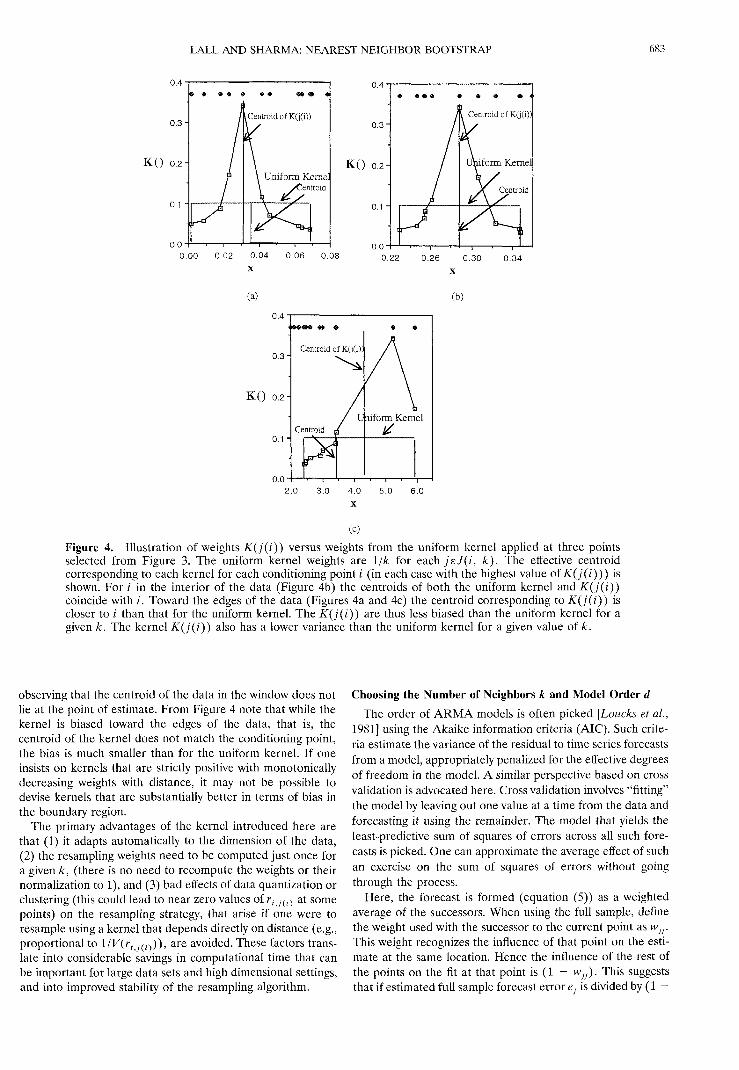
Figure 4. Illustration of weights K ( j ( i ) ) versus weights from the uniform kernel applied at three pointsselected from Figure 3. The uniform kernel weights are l/k for each jsJ(i, k). The effective centroidcorresponding to each kernel for each conditioning point / (in each case with the highest value of K ( j ( i ) ) ) isshown. For / in the interior of the data (Figure 4b) the centroids of both the uniform kernel and K ( j ( i ) )coincide with i. Toward the edges of the data (Figures 4a and 4c) the centroid corresponding to K ( j ( i ) ) iscloser to / than that for the uniform kernel. The K ( j ( i ) ) are thus less biased than the uniform kernel for agiven k. The kernel K ( j ( i ) ) also has a lower variance than the uniform kernel for a given value of k.

observing that the centroid of the data in the window does notlie at the point of estimate. From Figure 4 note that while thekernel is biased toward the edges of the data, that is, thecentroid of the kernel does not match the conditioning point,the bias is much smaller than for the uniform kernel. If oneinsists on kernels that are strictly positive with monotonicallydecreasing weights with distance, it may not be possible todevise kernels that are substantially better in terms of bias inthe boundary region.

The primary advantages of the kernel introduced here arethat (1) it adapts automatically to the dimension of the data,(2) the resampling weights need to be computed just once fora given k, (there is no need to recompute the weights or theirnormalization to 1), and (3) bad effects of data quantization orclustering (this could lead to near zero values of r- J(/) at somepoints) on the resampling strategy, that arise if one were toresample using a kernel that depends directly on distance (e.g.,proportional to \IV(rij^)), are avoided. These factors trans-late into considerable savings in computational time that canbe important for large data sets and high dimensional settings,and into improved stability of the resampling algorithm.

Choosing the Number of Neighbors k and Model Order dThe order of ARMA models is often picked [Loucks et al.,

1981] using the Akaike information criteria (AIC). Such crite-ria estimate the variance of the residual to time series forecastsfrom a model, appropriately penalized for the effective degreesof freedom in the model. A similar perspective based on crossvalidation is advocated here. Cross validation involves "fitting"the model by leaving out one value at a time from the data andforecasting it using the remainder. The model that yields theleast-predictive sum of squares of errors across all such fore-casts is picked. One can approximate the average effect of suchan exercise on the sum of squares of errors without goingthrough the process.

Here, the forecast is formed (equation (5)) as a weightedaverage of the successors. When using the full sample, definethe weight used with the successor to the current point as w7;.This weight recognizes the influence of that point on the esti-mate at the same location. Hence the influence of the rest ofthe points on the fit at that point is (1 - n>77). This suggeststhat if estimated full sample forecast error <?y is divided by (1 -


Table 1. Statistical Comparison of A;-nn and AR1 ModelSimulations Applied to an AR1 Sample

Simulations

5% Quantile Median95%

Quantile

AR1 Sample k-nn AR1 k-nn AR1 k-nn AR1

Mean 0.04Standard 1.11

deviationSkew -0.17Lag 1 0.63

correlation

-0.14 -0.12 0.02 0.041.02 1.03 1.10 1.11

0.24 0.201.18 1.20

-0.32 -0.25 -0.18 0.00 -0.03 0.210.56 0.57 0.62 0.63 0.68 0.69

Wjj), a measure of what the error may be if the data point (D7,Xj) was not used in developing the estimate is provided. Notethat the degrees of freedom (e.g., 0 for a k = 1 and 4/3 for ak = 3 using a uniform kernel) of estimate are implicit in thisidea. Craven and Wahba [1979] present a generalized crossvalidation (GCV) score function that considers the averageinfluence of excluded observations for estimation at each sam-ple point and approximates the predictive squared error ofestimate. The GCV score is given as

I e]ln

(8)

The GCV score function can be used to choose both k andd. For the kernel suggested in this paper, w;7 is a constant fora given k, and the GCV can be written as

GCV = (9)

A prescriptive choice of A: = nl/2 from experience is alsosuggested. This is a good choice for 1 < d < 6, and n > 100.Sensitivity to the choice of k in this neighborhood is small, andwhere computational resources are limited this choice can berecommended. Typically, with a sample size n of 50 to 200, thiscorresponds to a choice of A: ranging from 7 to 14. When usingthe GCV criteria with the same sample size, it is our experi-ence that varying k within 5 to 10 units of the optimal selectedvalue does not appreciably change the GCV score.

Criteria such as the GCV and the AIC are known to overfitor over parameterize time series relationships. With the near-est neighbor resampler, a model with order higher than nec-essary will have increased variability for a given k. The extra orsuperfluous coordinates serve to degrade rather than enhanceidentification of the patterns that describe the system. Like-wise, a smaller-than-optimal choice of d would lead to tracesthat lack the appropriate memory. Comparison of the at-tributes of the series generated by models with different valuesof A: and d is consequently desirable. These comparisons can bebased on how well attributes of direct interest to the investi-gator such as run lengths or the frequencies of threshold cross-

100Time

150

100

Time

150

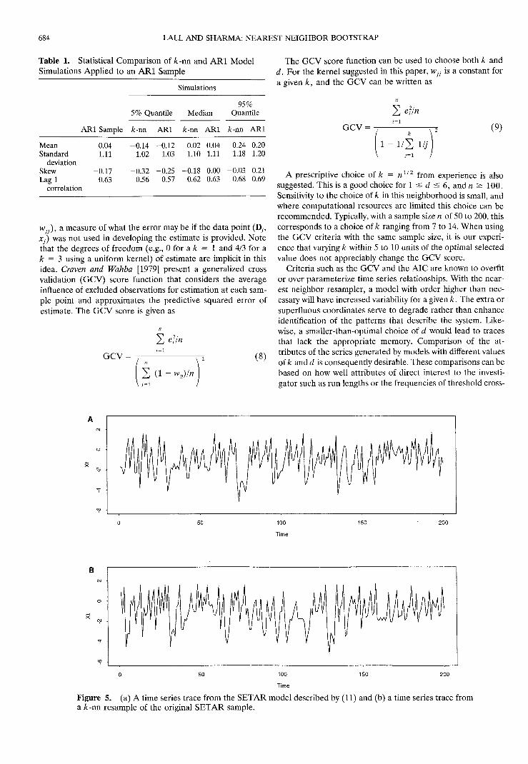
Figure 5. (a) A time series trace from the SETAR model described by (11) and (b) a time series trace froma A:-nn resample of the original SETAR sample.


Xt-1

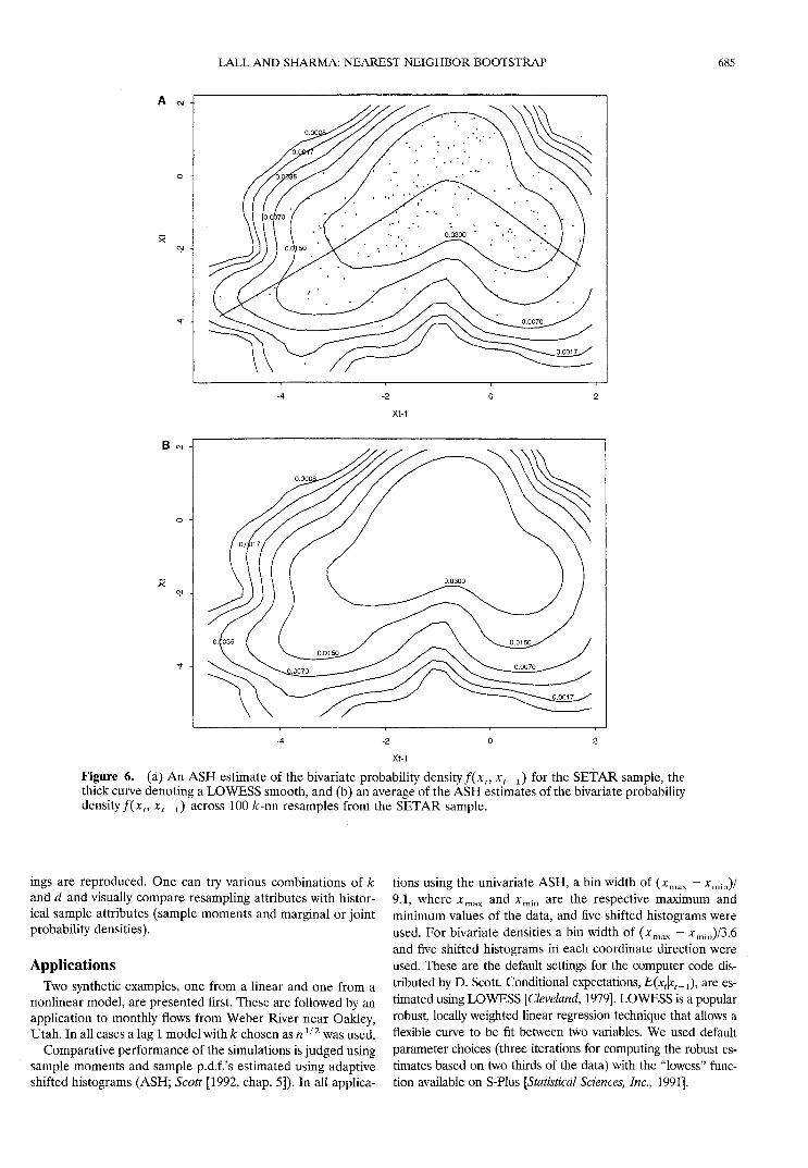
Figure 6. (a) An ASH estimate of the bivariate probability density f ( x t , *,_i) for the SETAR sample, thethick curve denoting a LOWESS smooth, and (b) an average of the ASH estimates of the bivariate probabilitydensity f(xt, xt_-^ across 100 /c-nn resamples from the SETAR sample.

ings are reproduced. One can try various combinations of kand d and visually compare resampling attributes with histor-ical sample attributes (sample moments and marginal or jointprobability densities).

ApplicationsTwo synthetic examples, one from a linear and one from a

nonlinear model, are presented first. These are followed by anapplication to monthly flows from Weber River near Oakley,Utah. In all cases a lag 1 model with k chosen as n1/2 was used.

Comparative performance of the simulations is judged usingsample moments and sample p.d.f.'s estimated using adaptiveshifted histograms (ASH; Scott [1992, chap. 5]). In all applica-

tions using the univariate ASH, a bin width of (*max - *min)/9.1, where xmax and *min are the respective maximum andminimum values of the data, and five shifted histograms wereused. For bivariate densities a bin width of (xmax - *min)/3.6and five shifted histograms in each coordinate direction wereused. These are the default settings for the computer code dis-tributed by D. Scott. Conditional expectations, E(xt\xt_1), are es-timated using LOWESS [Cleveland, 1979]. LOWESS is a popularrobust, locally weighted linear regression technique that allows aflexible curve to be fit between two variables. We used defaultparameter choices (three iterations for computing the robust es-timates based on two thirds of the data) with the "lowess" func-tion available on S-Plus [Statistical Sciences, Inc., 1991].


llill200 400 600

Time (months)

2 3 4 5 6 7 8 9 10 11 12

Time (months for year 2)

3 4 5 6 7 8 9 10 11 12

Time (months for year 29)

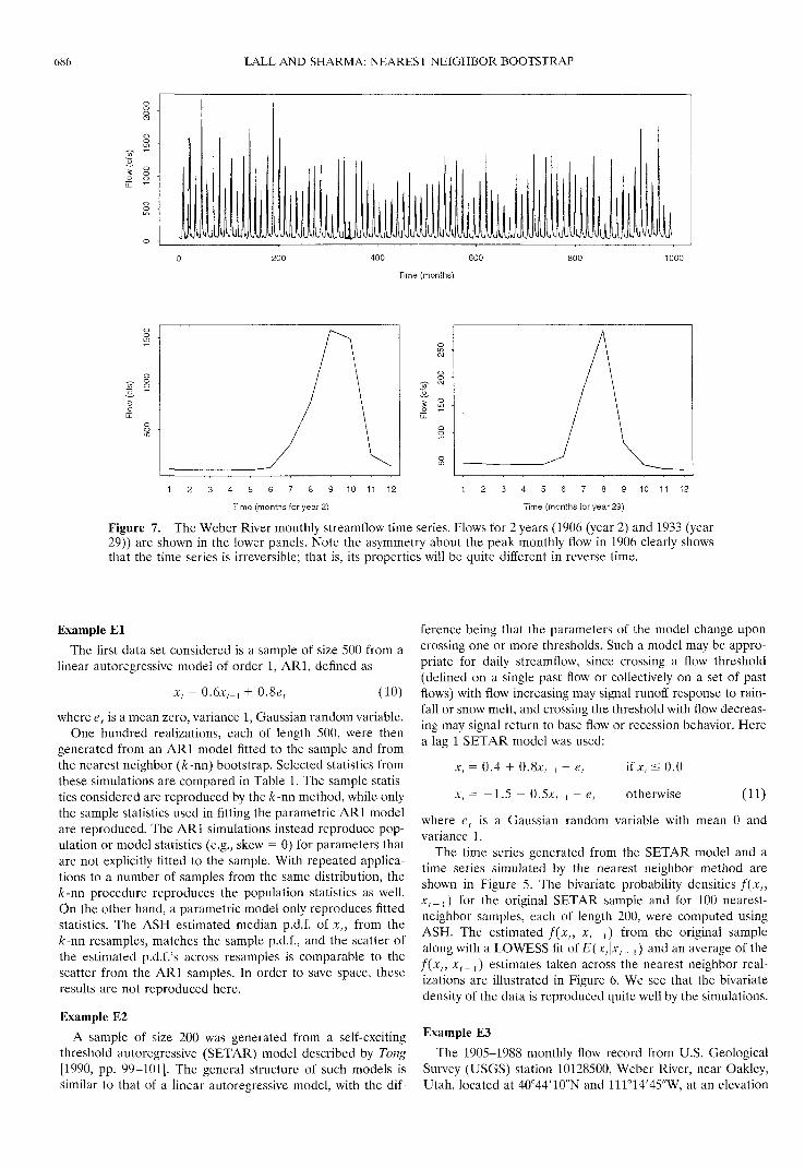
Figure 7. The Weber River monthly streamflow time series. Flows for 2 years (1906 (year 2) and 1933 (year29)) are shown in the lower panels. Note the asymmetry about the peak monthly flow in 1906 clearly showsthat the time series is irreversible; that is, its properties will be quite different in reverse time.

Example ElThe first data set considered is a sample of size 500 from a

linear autoregressive model of order 1, AR1, defined as

xt = (10)

where et is a mean zero, variance 1, Gaussian random variable.One hundred realizations, each of length 500, were then

generated from an AR1 model fitted to the sample and fromthe nearest neighbor (/c-nn) bootstrap. Selected statistics fromthese simulations are compared in Table 1. The sample statis-tics considered are reproduced by the /c-nn method, while onlythe sample statistics used in fitting the parametric AR1 modelare reproduced. The AR1 simulations instead reproduce pop-ulation or model statistics (e.g., skew = 0) for parameters thatare not explicitly fitted to the sample. With repeated applica-tions to a number of samples from the same distribution, theA:-nn procedure reproduces the population statistics as well.On the other hand, a parametric model only reproduces fittedstatistics. The ASH estimated median p.d.f. of xt, from the/c-nn resamples, matches the sample p.d.f., and the scatter ofthe estimated p.d.f.'s across resamples is comparable to thescatter from the AR1 samples. In order to save space, theseresults are not reproduced here.

Example E2A sample of size 200 was generated from a self-exciting

threshold autoregressive (SETAR) model described by Tong[1990, pp. 99-101]. The general structure of such models issimilar to that of a linear autoregressive model, with the dif-

ference being that the parameters of the model change uponcrossing one or more thresholds. Such a model may be appro-priate for daily streamflow, since crossing a flow threshold(defined on a single past flow or collectively on a set of pastflows) with flow increasing may signal runoff response to rain-fall or snow melt, and crossing the threshold with flow decreas-ing may signal return to base flow or recession behavior. Herea lag 1 SETAR model was used:

xt = 0.4 + 0.

xt = —1.5 —

*,-! + et

.5*,-! + e,

ifxt < 0.0

otherwise

where et is a Gaussian random variable with mean 0 andvariance 1.

The time series generated from the SETAR model and atime series simulated by the nearest neighbor method areshown in Figure 5. The bivariate probability densities f(xt,x t _ { ) for the original SETAR sample and for 100 nearest-neighbor samples, each of length 200, were computed usingASH. The estimated/(*,, xt_^ from the original samplealong with a LOWESS fit o f E ( x t \ x t _ l ) and an average of thef ( x t , x ( _ } ) estimates taken across the nearest neighbor real-izations are illustrated in Figure 6. We see that the bivariatedensity of the data is reproduced quite well by the simulations.

Example E3The 1905-1988 monthly flow record from U.S. Geological

Survey (USGS) station 10128500, Weber River, near Oakley,Utah, located at 40°44'10"N and 111°14'45"W, at an elevation


3L ^i ™u. ^c wCC^ CM^ CM

O O-1 CM

00

Q 0

~5 ^

Dec. Apr.

AR1

Aug. Ann.

Oct. Dec. Feb. Apr. Jun. Aug. Ann.

AR1

^w^3IT

V-NJ -

CM ̂

J

c\i c CM

"? CO*~ 0o

Apr.

k-nn

Aug.

Oct. Dec. Feb. Apr. Jun. Aug. Ann.

k-nn

W CM

Dec. Apr.

AR1

Aug.

co co

1OJ W CM

Apr.

k-nn

Aug.

Apr.

AR1

Aug. Ann.

o .oJS

Apr. Aug.

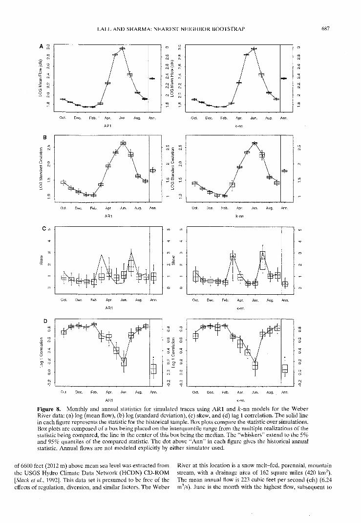
Figure 8. Monthly and annual statistics for simulated traces using AR1 and A:-nn models for the WeberRiver data: (a) log (mean flow), (b) log (standard deviation), (c) skew, and (d) lag 1 correlation. The solid linein each figure represents the statistic for the historical sample. Box plots compare the statistic over simulations.Box plots are composed of a box being placed on the interquantile range from the multiple realizations of thestatistic being compared, the line in the center of this box being the median. The "whiskers" extend to the 5%and 95% quantiles of the compared statistic. The dot above "Ann" in each figure gives the historical annualstatistic. Annual flows are not modeled explicitly by either simulator used.

of 6600 feet (2012 m) above mean sea level was extracted from River at this location is a snow melt-fed, perennial, mountainthe USGS Hydro Climate Data Network (HCDN) CD-ROM stream, with a drainage area of 162 square miles (420 km2).[Slack et al., 1992]. This data set is presumed to be free of the The mean annual flow is 223 cubic feet per second (cfs) (6.24effects of regulation, diversion, and similar factors. The Weber m3/s). June is the month with the highest flow, subsequent to

CL CD hrtCD &n_ N-.

i 8> '

O ft) J~

*S. £' 3'

!§- s?o S o ?,_, ^- cT o»TTJ l-{ P "•*

§'82 ?

Probability Density

0.0 0.005 0.015 0.025

Probability Density ^

0.0 0.005 0.015 0.025

CX)"* CL^ Ei CD

r^ O CDtJ^ CL EG.o Hi c?.

I *ZJ

8 'Tl

8

Probability Density

0.010 0.020

Sll

* gJ CL

Probability Density gg

0.010 0.020 0.030

§"5-5— ^- CL

n> PO

O3 P

@3 S-^^^ C/3 O£" a" po1 Q

Probability Density

0.0 0.0004 0.0008 0.0012

& S 8 § -^ S «-^ ^ 8v?3*^ o I"

cr »O ^x H-.

8 EC

Probability Density

0.0 0.0004 0.0008 0.0012O

I o

HOSHOIHN 1SHHV3N ^ QNV 1TV1


100 150

October

100 150

October

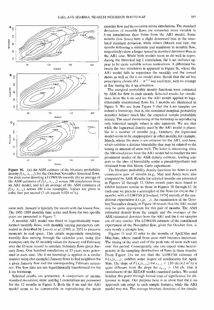
Figure 10. (a) An ASH estimate of the bivariate probabilitydensity f ( x t , x t _ ± ) for the October/November historical flows,the thick curve denoting a LOWESS smooth; (b) an average ofthe ASH estimates of/(;t,, xt_^ across 100 simulations froman ARl model; and (c) an average of the ASH estimates off(xf, Jc f_ 1 ) across 100 k-rm resamples. Values are given incubic feet per second (1 cfs equals 0.028 m3/s).

snow melt. January is typically the month with the lowest flow.The 1905-1988 monthly time series and flows for two specificyears are presented in Figure 7.

A monthly ARl model was fitted to logarithmically trans-formed monthly flows, with monthly varying parameters esti-mated as described by Loucks et al. [1981, p. 285] to preservemoments in real space. This entails sequentially simulatingmonthly flow moving through the calendar year, using (forexample) only the 83 monthly values for January and Februaryover the 83-year record to simulate February flows given Jan-uary flows. One hundred simulations of 83 years were gener-ated in each case. The A:-nn bootstrap is applied in a similarmanner using (for example) January flows to find neighbors fora given January flow and the corresponding February succes-sor. The flow data are not logarithmically transformed for thek-rm bootstrap.

Selected results are presented. A comparison of means,standard deviations, skew, and lag 1 correlations are presentedfor the 12 months in Figure 8. Both the k-rm and the ARlmodel seem to be comparable in reproducing the mean

monthly flow and its variation across simulations. The standarddeviations of monthly flows are somewhat more variable ink-rm simulations than those from the ARl model. Somemonths (low flows) have a slight downward bias in the simu-lated standard deviation, while others (March and July, themonths following a minimum and maximum in monthly flow,respectively) show a larger spread in standard deviation than inthe ARl case. While both models seem to do well in repro-ducing the historical lag 1 correlation, the k-rm statistics ap-pear to be more variable across realizations. A difference be-tween the two simulators is apparent in Figure 8c, where theARl model fails to reproduce the monthly and the annualskews as well as the k-rm model does. Recall that the ad hocprescriptive choice of A: = nl/2 was used here, with no attemptat fine tuning the k-rm simulator.

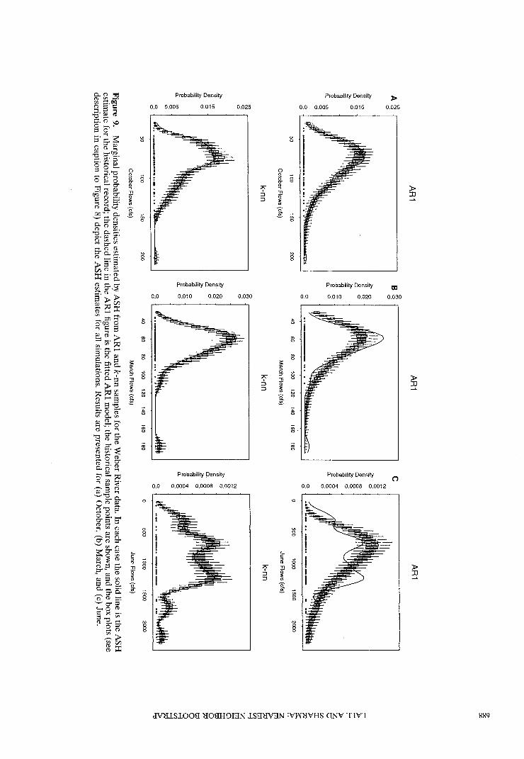
The marginal probability density functions were estimatedby ASH for flow in each month. Selected results for simula-tions from the k-rm and for the ARl model applied to loga-rithmically transformed flows for 3 months are illustrated inFigure 9. We see from Figure 9 that the k-rm samples areindeed a bootstrap; that is, the simulated marginal probabilitydensities behave much like the empirical sample probabilitydensity. The usual shortcoming of the bootstrap in reproducingonly historical sample values is also apparent. We see thatwhile the lognormal density used by the ARl model is plausi-ble in a number of months (e.g., October), the lognormalmodel seems to be inappropriate in other months, for example,March, where the skew is too extreme for the ARl, and June,which exhibits a distinct bimodality that may be related to thetiming or amount of snow melt. The latter is interesting, sincethe 100 simulations from the ARl model fail to bracket the twoprominent modes of the ASH density estimate, lending sup-port to the idea of bimodality under a pseudohypothesis testobtained from this Monte Carlo experiment.

The bivariate probability density functions for flows in eachconsecutive pair of months (e.g., May and June) were alsocomputed by ASH. Results for selected months are presentedin Figures 10 through 12. Other month pairs were found toexhibit features similar to those in Figures 10 through 12. Ineach case we present a scatterplot of the flows (in cfs) in the 2months, with a LOWESS [Cleveland, 1979] smooth of the con-ditional expectation E(xt\xt_1). An examination of the Octo-ber/November density in Figure 10 reveals that the ARl modelmay be quite appropriate for this pair of months. The ASHestimated density from the sample and the averages of theASH estimated densities from the ARl and the k-rm samplesare all very similar. The LOWESS estimate of the conditionalexpectation of the November flow, given the October flow, isvery nearly a straight line.

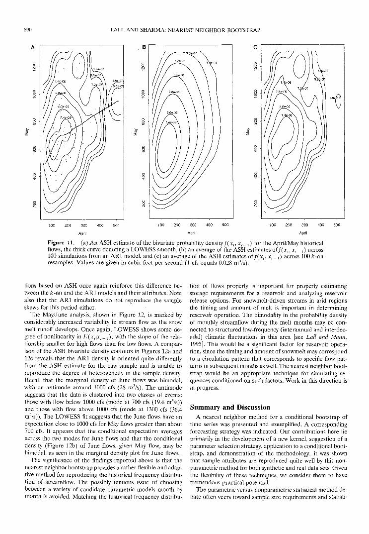
Figures 11 and 12 refer to the months of April/May andMay/June, where runoff from snow melt becomes important.The timing of the start and of the peak rate of snow melt varyover this period. Consequently, one can expect some hetero-geneity in the sampling distributions of flows in these months.From Figure lla we see that the LOWESS estimate ofE(xt\xt_1), exhibits some degree of nonlinearity for April/May. The slope o f E ( x t \ x t _ l ) for*,_! < 150 cfs (4.2 m3/s) isquite different from the slope for xt_l > 150 cfs. This isreminiscent of the SETAR model examined earlier. We couldbelabor this point through formal tests of significance for dif-ference in slope. Our purpose here is to show that the k-rmapproach can adapt to such sample features, while the ARlmodel may not. The average bivariate densities of the Simula-


100 200 300

April

300

April

400 500 200 300

April

500

Figure 11. (a) An ASH estimate of the bivariate probability density f(xt, x t _ ± ) for the April/May historicalflows, the thick curve denoting a LOWESS smooth, (b) an average of the ASH estimates of/(*,, xt_ x) across100 simulations from an AR1 model, and (c) an average of the ASH estimates off(xt, xt_ x) across 100 k-nnresamples. Values are given in cubic feet per second (1 cfs equals 0.028 m3/s).

tions based on ASH once again reinforce this difference be-tween the A;-nn and the AR1 models and their attributes. Notealso that the AR1 simulations do not reproduce the sampleskews for this period either.

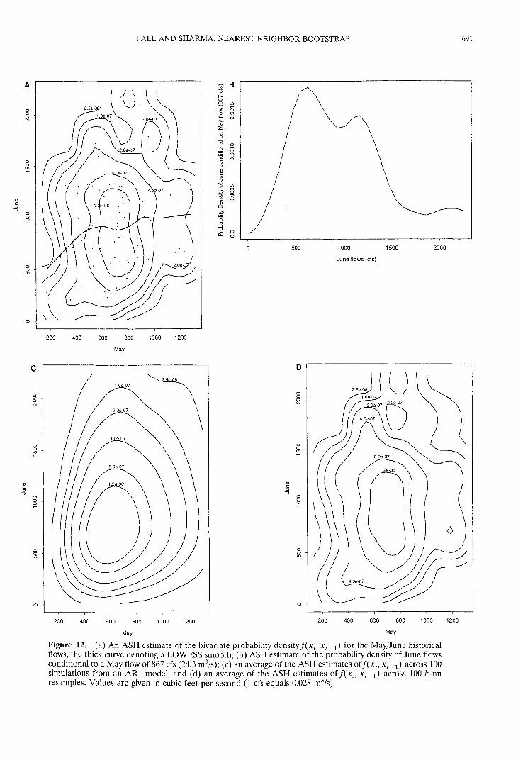
The May/June analysis, shown in Figure 12, is marked byconsiderably increased variability in stream flow as the snowmelt runoff develops. Once again, LOWESS shows some de-gree of nonlinearity in E(xt\xt_1), with the slope of the rela-tionship smaller for high flows than for low flows. A compar-ison of the ASH bivariate density contours in Figures 12a and12c reveals that the AR1 density is oriented quite differentlyfrom the ASH estimate for the raw sample and is unable toreproduce the degree of heterogeneity in the sample density.Recall that the marginal density of June flows was bimodal,with an antimode around 1000 cfs (28 m3/s). The antimodesuggests that the data is clustered into two classes of events:those with flow below 1000 cfs (mode at 700 cfs (19.6 m3/s))and those with flow above 1000 cfs (mode at 1300 cfs (36.4m3/s)). The LOWESS fit suggests that the June flows have anexpectation close to 1000 cfs for May flows greater than about700 cfs. It appears that the conditional expectation averagesacross the two modes for June flows and that the conditionaldensity (Figure 12b) of June flows, given May flow, may bebimodal, as seen in the marginal density plot for June flows.

The significance of the findings reported above is that thenearest neighbor bootstrap provides a rather flexible and adap-tive method for reproducing the historical frequency distribu-tion of streamflow. The possibly tenuous issue of choosingbetween a variety of candidate parametric models month bymonth is avoided. Matching the historical frequency distribu-

tion of flows properly is important for properly estimatingstorage requirements for a reservoir and analyzing reservoirrelease options. For snowmelt-driven streams in arid regionsthe timing and amount of melt is important in determiningreservoir operation. The bimodality in the probability densityof monthly streamflow during the melt months may be con-nected to structured low-frequency (interannual and interdec-adal) climatic fluctuations in this area [see Lall and Mann,1995]. This would be a significant factor for reservoir opera-tion, since the timing and amount of snowmelt may correspondto a circulation pattern that corresponds to specific flow pat-terns in subsequent months as well. The nearest neighbor boot-strap would be an appropriate technique for simulating se-quences conditioned on such factors. Work in this direction isin progress.

Summary and DiscussionA nearest neighbor method for a conditional bootstrap of

time series was presented and exemplified. A correspondingforecasting strategy was indicated. Our contributions here lieprimarily in the development of a new kernel, suggestion of aparameter selection strategy, application to a conditional boot-strap, and demonstration of the methodology. It was shownthat sample attributes are reproduced quite well by this non-parametric method for both synthetic and real data sets. Giventhe flexibility of these techniques, we consider them to havetremendous practical potential.

The parametric versus nonparametric statistical method de-bate often veers toward sample size requirements and statisti-


\

500 1000 1500

June flows (cfs)

2000

200 400 600 800 1000 1200

May

200 800 1000 1200 200 800 1000 1200

May May

Figure 12. (a) An ASH estimate of the bivariate probability density f(xt, * r_ x) for the May/June historicalflows, the thick curve denoting a LOWESS smooth; (b) ASH estimate of the probability density of June flowsconditional to a May flow of 867 cfs (24.3 m3/s); (c) an average of the ASH estimates off(xt, x t _ ± ) across 100simulations from an AR1 model; and (d) an average of the ASH estimates off(xf, xf_^ across 100 k-rmresamples. Values are given in cubic feet per second (1 cfs equals 0.028 m3/s).


cal efficiency arguments. In the context of a resampling strat-egy, as espoused here, these arguments take a somewhatdifferent complexion. For some processes, such as dailystreamflow, identification or even definition of an appropriateparametric model is problematic. In these cases, data are rel-atively plentiful. For such cases, methods such as those pre-sented here are enticing. For monthly and annual flows, thereis progressively less structure, and sample sizes are smaller. Inthese situations, parametric methods may indeed be statisti-cally more efficient provided the correct model is identifiableand parsimonious. In our view, particularly for the snow-fedrivers of the western United States, this may not always be thecase. Indeed, for the application presented here at the monthlytimescale it is hard to justify choosing the parametric approachover the nearest neighbor method. The consideration of pa-rameter uncertainty is justifiably considered a good idea inparametric time series resampling of streamflow [Grygier andStedinger, 1990]. Likewise it may be useful to think aboutmodel uncertainty when developing parametric models. Thelatter consideration is implicit in the nonparametric approach,since a rather broad class of models is approximated. Theimpact of varying the "parameters" k and the model order onspecific attributes of the resamples bears further investigation.Our preliminary analyses suggest that the sensitivity of thescheme is limited over a range of k values near the "optimal"with the kernel used here. Formal investigations of this issueare being pursued.

One can devise a strategy that allows nearest neighbor re-sampling with perturbation of the historical data in the spirit oftraditional autoregressive models, that is, conditional expecta-tion with an added random innovation. First, one evaluates theconditional expectation using the generalized nearest neighborregression estimator for each vector D, in the historical record.A residual et can be computed as the difference between thesuccessor *; of D, and the nearest neighbor regression forecast.The simulation proceeds by estimating the nearest neighborregression forecast relative to a conditioning vector D, andthen adding to this one of the <?y corresponding to a data pointj that lie in the k nearest neighborhood Jt k. The innovation e^is chosen using the resampling kernel K ( j ( i ) ) . This schemewill perturb the historical data points in the series, with inno-vations that are representative of the neighborhood, and willthus "fill in" between the historical data values as well asextrapolating beyond the sample. The computational burden isincreased and there is a possibility that the bounds on thevariables will be violated during simulation. However, theremay be situations where the investigator may wish to adopt thisstrategy. Further exploration of this strategy is planned.

Issues such as disaggregation of streamflows bear furtherinvestigation. One strategy is trivial: resample the flow vectorthat aggregates to the aggregate flow simulated. A questionthat arises is whether there is even any need to work withmodels that disaggregate (especially in time) using these meth-ods. One may wish to work directly with, say, the daily flows,conditioned on a sequence of past daily flows and weekly ormonthly flows.

The real utility of the method presented here may lie inexploiting a dependence structure (e.g., in daily flows) that isdifficult to treat by traditional methods, as well as complexrelationships between variables, and in estimating confidencelimits or risk in problems that have a time series structure. Thetraditional time series analysis framework directs the research-er's attention toward an efficient estimation of model param-

eters under some metric (e.g., least squares or maximum like-lihood). The performance metric of interest to the hydrologistmay not be the one optimal for the estimation of a certain setof parameters and selected model form. There is reason todirectly explore other aspects of the problem that may be ofdirect interest for reservoir operation and flood control, usingflexible, adaptive, data exploratory methods. Such investiga-tions using the /c-nn bootstrap are in progress.

Acknowledgments. The work reported here was supported in partby the USGS through grant number 1434-92-G-2265. Discussions withand review of this work by David Tarboton are acknowledged. Thecomments of the anonymous reviewers resulted in a significant im-provement of the manuscript.

ReferencesCleveland, W. S., Robust locally weighted regression and smoothing

scatterplots, /. Am. Stat. Assoc., 74, 829-836, 1979.Craven, P., and G. Wahba, Smoothing noisy data with spline functions,

Numer. Math., 31, 377-403, 1979.Efron, B., Bootstrap methods: Another look at the Jacknknife, Ann.

Stat., 7, 1-26, 1979.Efron, B., and R. Tibishirani, An Introduction to the Bootstrap, Chap-

man and Hall, New York, 1993.Eubank, R. L., Spline Smoothing and Nonparametric Regression, Statis-

tics: Textbooks and Monographs, Marcel Dekker, New York, 1988.Grygier, J. C, and J. R. Stedinger, Spigot, a synthetic streamflow

generation package, technical description, version 2.5, School of Civ.and Environ. Eng., Cornell Univ., Ithaca, N. Y., 1990.

Gyorfi, L., W. Hardle, P. Sarda, and P. Vieu, Nonparametric CurveEstimation from Time Series, vol. 60, Lecture Notes in Statistics,Springer-Verlag, New York, 1989.

Hardle, W., Applied Nonparametric Regression, Econometric Soc.Monogr., Cambridge Univ. Press, New York, 1989.

Hardle, W., Smoothing Techniques With Implementation in S, Springer-Verlag, New York, 1990.

Hardle, W., and A. W. Bowman, Bootstrapping in nonparametricregression: Local adaptive smoothing and confidence bands, /. Am.Stat. Assoc., 83, 102-110, 1988.

Karlsson, M., and S. Yakowitz, Nearest-Neighbor methods for non-parametric rainfall-runoff forecasting, Water Resour. Res., 23, 1300-1308, 1987a.

Karlsson, M., and S. Yakowitz, Rainfall-runoff forecasting methods,old and new, Stochastic Hydrol. Hydraul., J, 303-318, 1987b.

Kendall, D. R., and J. A. Dracup, A comparison of index-sequentialand AR(1) generated hydrologic sequences,/ Hydrol., 122, 335-352,1991.

Kunsch, H. R., The Jackknife and the Bootstrap for General Station-ary Observations, ,4wL Stat., 17, 1217-1241, 1989.

Lall, U., Nonparametric function estimation: Recent hydrologic appli-cations, U.S. Natl. Rep. Int. Union Geod. Geophys. 1991-1994, Rev.Geophys., 33, 1093, 1995.

Lall, U., and M. Mann, The Great Salt Lake: A barometer of low-frequency climate variability, Water Resour. Res., 31(W), 2503-2515,1995.

Loucks, D. P., J. R. Stedinger, and D. A. Haith, Water Resource SystemsPlanning and Analysis, 559 pp., Prentice-Hall, Englewood Cliffs,N. J., 1981.

Schuster, E., and S. Yakowitz, Contributions to the theory of nonpara-metric regression, with application to system identification, Ann.Stat., 7, 139-149, 1979.

Scott, D. W., Multivariate Density Estimation: Theory, Practice andVisualization, John Wiley, New York, 1992.

Silverman, B. W., Density Estimation for Statistics and Data Analysis,Chapman and Hall, New York, 1986.

Slack, J. R., J. M. Landwehr, and A. Lumb, A U.S. Geological Surveystreamflow data set for the United States for the study of climatevariations, 1874-1988, Rep. 92-129, U.S. Geol. Surv., Oakley, Utah,1992.

Smith, J. A., Long-range streamflow forecasting using nonparametricregression, Water Resour. Bull., 27, 39-46, 1991.

Smith, J., G. N. Day, and M. D. Kane, Nonparametric framework for


long range streamflow forecasting, /. Water Resour. Plann. Manage.,118, 82-92, 1992.

Statistical Sciences, Inc., S-Plus Reference Manual, Version 3.0, Seattle,Wash., 1991.

Tarboton, D. G., A. Sharma, and U. Lall, The use of non-parametricprobability distributions in streamflow modeling, in Proceedings ofthe Sixth South African National Hydrological Symposium, ed. S. A.Lorentz et al., University of Natal, Pietermaritzburg, South Africa,September 8-10, 315-327, 1993.

Tasker, G. D., Comparison of methods for estimating low flow char-acteristics of streams, Water Resour. Bull, 23, 1077-1083, 1987.

Tong, H., Nonlinear Time Series Analysis: A Dynamical Systems Per-spective, Academic, San Diego, Calif., 1990.

Woo, M. K., Confidence intervals of optimal risk-based hydraulic de-sign parameters, Can. Water Resour. J., 14, 10-16, 1989.

Yakowitz, S., A stochastic model for daily river flows in an arid region,Water Resour. Res., 9, 1271-1285, 1973.

Yakowitz, S., Nonparametric estimation of markov transition func-tions, Ann. Stat., 7, 671-679, 1979.

Yakowitz, S. J., Nonparametric density estimation, prediction, and

regression for markov sequences, /. Am. Stat. Assoc., 80, 215-221,1985.

Yakowitz, S., Nearest-neighbor regression estimation for null-recurrent Markov time series, Stochastic Processes Their Appl., 48,311-318, 1993,

Yakowitz, S., and M. Karlsson, Nearest-neighbor methods with appli-cation to rainfall/runoff prediction, in Stochastic Hydrology, edited byJ. B. Macneil and G. J. Humphries, pp. 149-160, D. Reidel, Norwell,Mass., 1987.

Zucchini, W., and P. T. Adamson, Bootstrap confidence intervals fordesign storms from exceedance series, Hydrol. Sci. J., 34, 41-48,1989.

U. Lall and A. Sharma, Utah Water Research Laboratory, UtahState University, UMC82, Logan, UT 84322-8200. (e-mail: ulall®kernel.uwrl.usu.edu; [email protected])

(Received February 23, 1995; revised September 20, 1995;accepted September 22, 1995.)

Documents

A nearest neighbor bootstrap for resampling hydrologic …civil.colorado.edu/~balajir/Adv-Data-material/CVEN-6833/papers-2... · WATER RESOURCES RESEARCH, VOL. 32, NO. 3, PAGES 679-693,