NBER WORKING PAPER SERIES

A NATION OF IMMIGRANTS:ASSIMILATION AND ECONOMIC OUTCOMES IN THE AGE OF MASS MIGRATION

Ran AbramitzkyLeah Platt BoustanKatherine Eriksson

Working Paper 18011http://www.nber.org/papers/w18011

NATIONAL BUREAU OF ECONOMIC RESEARCH1050 Massachusetts Avenue

Cambridge, MA 02138April 2012

We are grateful for the access to Census manuscripts provided by Ancestry.com and FamilySearch.org.We benefited from the helpful comments of participants at the UC-Davis Interdisciplinary Conferenceon Social Mobility, the AFD-World Bank Migration and Development Conference, the Labor Markets,Families and Children conference at the University of Stavanger, the Economic History Association,and the NBER Development of the American Economy Summer Institute. We also thank participantsof seminars at Berkeley, Caltech, Chicago, Duke, Hebrew University, Northwestern, Norwegian Schoolof Economics, Stanford, Tel Aviv, UC-Davis, UCLA, and UT-Austin. We benefited from conversationswith Manuel Amador, Attila Ambrus, Pat Bayer, Doug Bernheim, Tim Bresnahan, Marianne Bertrand,David Card, Greg Clark, Dora Costa, Pascaline Dupas, Liran Einav, Joseph Ferrie, Erica Field, DoireannFitzgerald, Bob Gordon, Avner Greif, Hilary Hoynes, Nir Jaimovich, Lawrence Katz, Pete Klenow,Pablo Kurlat, Aprajit Mahajan, Robert Margo, Daniel McGarry, Roy Mill, Joel Mokyr, Jean-LaurentRosenthal, Seth Sanders, Izi Sin, Yannay Spitzer, Gui Woolston, Gavin Wright, and members of theUCLA KALER group. Roy Mill provided able assistance with data collection. We acknowledge financialsupport from the National Science Foundation (No. SES-0720901), the California Center for PopulationResearch and UCLA’s Center for Economic History. The views expressed herein are those of the authorsand do not necessarily reflect the views of the National Bureau of Economic Research.

NBER working papers are circulated for discussion and comment purposes. They have not been peer-reviewed or been subject to the review by the NBER Board of Directors that accompanies officialNBER publications.

© 2012 by Ran Abramitzky, Leah Platt Boustan, and Katherine Eriksson. All rights reserved. Shortsections of text, not to exceed two paragraphs, may be quoted without explicit permission providedthat full credit, including © notice, is given to the source.

A Nation of Immigrants: Assimilation and Economic Outcomes in the Age of Mass MigrationRan Abramitzky, Leah Platt Boustan, and Katherine ErikssonNBER Working Paper No. 18011April 2012, Revised August 2013JEL No. F22,J61,N31

ABSTRACT

During the Age of Mass Migration (1850-1913), the US maintained an open border, absorbing 30million European immigrants. Prior cross-sectional work on this era finds that immigrants initiallyheld lower-paid occupations than natives but experienced rapid convergence over time. In newly-assembledpanel data, we show that, in fact, the average immigrant did not face a substantial occupation-basedearnings penalty upon first arrival and experienced occupational advancement at the same rate as natives.Cross-sectional patterns are driven by biases from declining arrival cohort quality and departures ofnegatively-selected return migrants. We show that assimilation patterns vary substantially across sendingcountries and persist in the second generation.

Ran AbramitzkyDepartment of EconomicsStanford University579 Serra MallStanford, CA 94305and NBERranabr@stanford.edu

Leah Platt BoustanDepartment of Economics8283 Bunche HallUCLALos Angeles, CA 90095-1477and NBERlboustan@econ.ucla.edu

Katherine ErikssonDepartment of Economics8283 Bunche HallUCLALos Angeles, CA 90095-1477kath722@ucla.edu

  1

I. Introduction

We study the assimilation of European immigrants in the United States labor market

during the Age of Mass Migration (1850-1913), one of the largest migration episodes in modern

history. Almost thirty million immigrants moved to the US during this period; by 1910, 22

percent of the US labor force was foreign born, compared with only 17 percent today. At the

time, US borders were completely open to European immigrants. Yet, much like today,

contemporaries were concerned about the ability of migrants to assimilate into the US economy.

Congress fought with various presidential administrations about whether to tighten immigration

policies for over thirty years before finally imposing strict quotas in 1924, putting an end to the

era of open borders.

Our paper challenges conventional wisdom and prior research about immigrant

assimilation during this period.1 The common view is that European immigrants held

substantially lower-paid occupations than natives upon first arrival, but that they converged with

the native born after spending some time in the US.2 Using newly-assembled panel data for

21,000 natives and immigrants from 16 sending European countries, we instead find that, on

average, long term immigrants from sending countries with real wages above the European

median actually held significantly higher-paid occupations than US natives upon first arrival,

while immigrants from sending countries with below-median wages started out in equal or

                                                            1 For example, politicians and commentators often assume that even uneducated European immigrant groups were able to achieve economic success within a generation or two. Sowell (1996) gives expression to this view, writing that “although notoriously uneducated and illiterate... Southern and Eastern Europeans eventually became… well-represented in occupations requiring education” (p. 48). In contrast, observers often divide contemporary immigrant groups into those that assimilate quickly and those that do not, as typified by Huntington’s (2004) assessment that “immigrants from India, Korea, Japan and the Philippines, whose educational profiles more closely approximate those of native Americans, have generally assimilated rapidly... [while] Latin American immigrants, particularly those from Mexico, and their descendants have been slower in approximating American norms” (p. 187-88). 2 Following the economics literature, we focus on immigrants’ labor market performance, rather than on other measures of cultural or social assimilation. In particular, we discuss occupational attainment because individual earnings were not recorded in population Censuses before the mid-twentieth century.

  2

lower-paid occupations.3 We find little evidence for the commonly held view that immigrants

converged with natives, but rather document substantial persistence of the initial earnings gap

between immigrants and natives (whether positive or negative) over the lifecycle. In other words,

regardless of starting point, immigrants experienced occupational upgrading similar to natives,

thereby preserving the initial gaps between immigrants and natives over time. Furthermore, this

gap persisted into the second generation; when migrants from a certain source country

outperformed US natives, so did second generation migrants, and vice versa.4

Prior studies used cross-sectional data, which confounds immigrant convergence to

natives in the labor market with immigrant arrival cohort effects and the selection of return

migrants from the migrant pool. Indeed, when we use cross sectional data, we confirm the

findings of prior studies. When contrasting these findings with those using our panel data, we

conclude that the apparent convergence in a single cross-section is driven by a decline in the

quality of immigrant cohorts over time and the departure of negatively-selected return migrants

(see Borjas, 1985 and Lubotsky, 2007 for discussions of these sources of bias in contemporary

data).5

We conclude that the notion that immigrants faced a large initial occupational penalty

during the historical Age of Mass Migration is overstated. Even when US borders were open, the

average immigrant who ended up settling in the US long term held occupations that commanded

                                                            3 We follow individuals between the 1900, 1910, and 1920 US Censuses by using their name, age, and place of birth. Assembling such panel data is possible because US Census policy makes complete individual records (including names) publicly available after 72 years. In particular, we link immigrants and US natives from the 1900 Census manuscripts to the 1910 and 1920 Census manuscripts using the genealogy websites Ancestry.com and FamilySearch.org. 4 Occupational differences may have persisted over generations because children of migrants grew up in migrant enclaves, inherited skills from their parents, or used their parents’ networks to find jobs. 5 Over 25 percent of migrants returned to Europe during this era (Gould, 1980; Bandiera, Rasul and Viarengo, 2013). Return migrants may have been negatively selected because those who were unsuccessful in the US returned home. In addition, many migrants in this era employed a deliberate strategy of temporary migration to the New World (Piore, 1980; Wyman, 1996). These temporary migrants will likely appear to be negatively selected using our occupation-based measures if they remained in low-paid occupations during their short sojourn (Dustmann, 1993).

  3

similar pay to US natives upon first arrival.6 These findings suggest that migration restrictions or

selection policies are not necessary to ensure strong migrants’ performance in the labor market.

At the same time, the notion that European immigrants converged with natives after

spending 10 to 15 years in the US is also exaggerated, as we find that initial immigrant-native

occupational gaps persisted over time and even across generations. This pattern casts doubt on

the conventional view that, in the past, immigrants who arrived with few skills were able to

invest in themselves and succeed in the US economy within a single generation.

The remainder of the paper proceeds as follows. Section 2 discusses the historical context

and related literature. Section 3 reviews methods used to infer immigrant assimilation in cross-

sectional and panel data settings and the biases associated with each. In Section 4, we describe

the data construction and matching procedures. Section 5 presents our empirical strategy and

main results on immigrant assimilation and the selection of return migrants. Section 6 contains

country-by-country results on assimilation and return migration. In Section 7, we assess the

robustness of our main findings and present occupational transition matrices that provide more

detail about how immigrants and natives moved up the occupational ladder over time. Section 8

rules out other sources of selective attrition from the panel sample beyond return migration,

including selective mortality or names changes. Section 9 analyzes the performance of second-

generation immigrants relative to their parents and Section 10 concludes.

II. Immigrant assimilation in the early 20th century: Historical context and related literature

The US absorbed 30 million migrants during the Age of Mass Migration (1850-1913). By

1910, 22 percent of the US labor force – and 38 percent of workers in non-southern cities – were

                                                            6 Immigrants were more likely than natives to settle in states with a high-paying mix of occupations; location choice was an important strategy that immigrants used to achieve occupational parity with natives.

  4

foreign-born (compared with 17 percent today).7 Over the period, migrant-sending countries

shifted toward the poorer regions of southern and eastern Europe (Hatton and Williamson, 1998).

Many contemporary observers expressed concerns about the concentrated poverty in immigrant

neighborhoods and the low levels of education among immigrant children, many of whom left

school at young ages in order to work in textiles and manufacturing (Muller, 1993; Moehling,

1999). Prompted by these concerns, progressive reformers championed a series of private

initiatives and public legislation, including child labor laws and compulsory schooling

requirements, to facilitate immigrant absorption (Lleras-Muney, 2002; Carter, 2008; Lleras-

Muney and Shertzer, 2011), while nativists instead believed that new arrivals would never be

able to fit into American society (Higham, 1988; Jacobson, 1999).

Fears about immigrant assimilation encouraged Congress to convene a special

commission in 1907 to study the social and economic conditions of the immigrant population.

The resulting report concluded that immigrants, particularly from southern and eastern Europe

would be unable to assimilate, in part because of high rates of temporary and return migration.8

The Immigration Commission report provided fuel for legislators seeking to restrict immigrant

entry (Benton-Cohen, 2010). In 1917, Congress passed a literacy test, which required potential

immigrants to demonstrate the ability to read and write in any language (Goldin, 1994). In 1924,

Congress further restricted immigrant entry by setting a strict quota of 150,000 arrivals per year,

with more slots allocated to northern and western European countries.

                                                            7 Authors’ calculations using the 1910 Integrated Public Use Microdata Series (IPUMS). 8 Two authors of the report, Jeremiah Jenks and W. Jett Lauck, later summarized this view of temporary migrants, writing: “if an immigrant intends to remain permanently in the US and become an American citizen, he naturally begins at once… to fit himself for the conditions of his new life…If, on the other hand, he intends his sojourn in this country to be short… the acquisition of the English language will be of little consequence… The chief aim of a person with this intention is to put money in his purse… not for investment here but for investment in his home country” (quoted in Wyman, 1996, p. 99-100).

  5

Since the publication of the Immigration Commission report, generations of economists

and economic historians have assessed the labor market performance of this large wave of

immigrant arrivals.9 The earliest studies in this area (re-)analyzed the aggregate wage data

published by the Immigration Commission and find that, contrary to the initial conclusions of the

commission, immigrants caught up with the native-born after 10 to 20 years in the US (Higgs,

1971; McGoldrick and Tannen, 1977; Blau, 1980). Related work examined individual-level

wage data from surveys conducted by State Labor Bureaus (Hannon, 1982; Eichengreen and

Gemery, 1986; Hanes, 1996). Although early studies of these sources found no wage

convergence, Hatton (1997) argues that this discrepancy is due to specification choice. He re-

analyzes the state data with two simple modifications and finds that immigrants who arrived at

age 25 fully erased the wage gap with natives within 13 years in the US.10

More recent studies on immigrant assimilation incorporate data from the federal Census

of Population. The Census offers complete industrial and geographic coverage but only contains

information on occupation, rather than individual wages or earnings. Relying on the 1900 and

1910 Census cross sections, Minns (2000) finds partial convergence between immigrants and

natives outside of the agricultural sector.11 Immigrants eliminate 30 to 40 percent of their

(between-occupation) earnings deficit relative to natives after 15 years in the US.

                                                            9 In a related body of work, Ferrie (1997, 1999) measures immigrant assimilation in the Antebellum period. Lieberson (1980) and Alba and Nee (2003) are two core references in the sociological literature on immigrant assimilation. 10 In particular, Hatton (1997) allows for differences in the return to experience for younger and older workers and separates immigrants who arrived as children from those who arrived as adults. The convergence figure reported in the text is based on Hatton (1997, Table 4, columns 1 and 3). Because Hatton estimates different returns to experience parameters for immigrants and the native born, the size of the initial wage gap varies by age. For this calculation, we consider an immigrant who arrives at age 25, at which point the implied wage gap with natives is 0.275, a gap which is erased after the immigrant spends 13 years in the US. 11 Consistent with our results, Minns finds that the full immigrant population actually earn as much as (or more than) natives. The immigrant deficit explored in his paper is present only outside of the agricultural sector.

  6

Overall, across three different datasets, the existing literature suggests that immigrant

workers experienced substantial occupational and earnings convergence with the native-born in

the early twentieth century. However, all these analyses compare earnings in a single cross

section, a method that suffers from two potentially important sources of bias: selective return

migration, and changes in immigrant cohort quality over time.12

III. Inferring immigrant assimilation from cross sectional and panel data

Imagine that the researcher only has a single cross section of data, say the 1920 Census,

from which to estimate the pace of convergence between immigrants and the native born in the

labor market. In this case, she may compare the earnings of a long-standing immigrant who

arrived in the US in 1895 to that of a recent immigrant who arrived in 1915. For illustration, let

the mean earnings of a native-born worker be 100 dollars. If the immigrant who arrived in 1895

also earned 100 dollars in 1920, while the immigrant who arrived in 1915 earned 50 dollars, the

researcher could conclude that, upon arrival, migrants faced an earning penalty relative to natives

that is completely erased after 25 years in the US. However, this conclusion might mistake

differential skills across arrival cohorts for true migrant assimilation; this point was first made by

Douglas (1919) and was developed by Borjas (1985).13 If, for example, the long-standing

migrant was a literate craftsman from Germany, whereas the recent arrival was an unskilled

common laborer from Italy, the difference in their earnings in 1920 may reflect permanent gaps

in their skill levels rather than temporary gaps due to varying time spent in the US.

                                                            12 Minns (2000) acknowledges the potential bias from changes in the quality of immigrant arrival cohorts. Hatton (1997) partially addressed the shift in sending countries by separately analyzing assimilation profiles by country of origin for three sending countries (Britain, Ireland and Germany). 13 In an early paper in this literature, Chiswick (1978) found that immigrants in the 1970 cross section experienced faster wage growth than the native-born and overtook natives within 15 years of arrival. Borjas (1985) demonstrated that, in this period, half of the apparent convergence in a cross section is driven by changes in cohort quality over time.

  7

This bias can be addressed with repeated cross-sectional observations on arrival cohorts,

say by observing 1895 immigrant arrivals in both the 1900 and 1920 Censuses. However, in this

case, inferences on migrant assimilation may still be inaccurate due to selective return migration;

this point was first made by Jasso and Rosenzweig (1988) and was investigated empirically by

Lubotksy (2007).14 In the 1900 census, the 1895 migrant arrival cohort contains both temporary

arrivals who will return to their home country before the 1920 census and longer-standing

immigrants who will remain in the US in 1920. By 1920, only the long-standing immigrants

remain. If the temporary migrants have lower skills or exert less effort in moving up the

occupational ladder in the US, this compositional change in the repeated cross section will

generate the appearance of wage growth within the cohort over time as the lower-earning

migrants return to Europe.15

We emphasize that in our panel data we estimate an assimilation profile for immigrants

who were in the US in both 1900 and 1920 – that is, those who remained in the US for at least 20

years. These immigrants are of particular interest because they participate in the US labor market

for many years and are more likely to raise children in the US who then contribute to the labor

force in the next generation. However, to understand the experience of the typical migrant in the

US at a point in time, a group that includes both permanent migrants and migrants who will later

return to their home country, the assimilation patterns in the repeated cross sections are also of

interest.

                                                            14 During the Age of Mass Migration, some immigrants engaged in circular migration, migrating to the US and returning to Europe multiple times (Piore, 1980; Wyman, 1996). Circular migrants will enter the panel sample only if they happen to live in the US on the Census years; otherwise, they will be treated as temporary migrants. 15 In addition to Lubotsky (2007), other panel analyses of immigrant assimilation in the contemporary period include Borjas (1989), Hu (2000), Edin, Lalonde and Aslund (2000), Duleep and Dowhan (2002), Constant and Massey (2003), Eckstein and Weiss (2004) and Kim (2011). Zakharenko (2008) provides descriptive evidence that return migrants leaving the US are negatively selected.

  8

In an earlier paper, we compiled a panel dataset of immigrants that matched individuals

from their childhood household in Europe to their adult outcomes; in this case, we were only

able to focus on a single sending country, Norway (Abramitzky, Boustan and Eriksson, 2012).

These data allowed us to analyze the selection of who migrates from Europe to the United States

and the economic return to this migration. We found evidence of negative selection, in the sense

that men whose fathers did not own land or whose fathers held low-skilled occupations were

more likely to migrate. We also estimated a return to migration free from between-household

selection by comparing brothers, one of whom migrated and one of whom stayed in Norway;

using this method, we found a return to migration of around 70 percent. In this paper, we use

panel data to compare immigrants to US natives (assimilation), rather than to compare

immigrants to the European sending population (selection). Furthermore, we move beyond our

focus on a single country and assemble new panel data for immigrants from 16 sending

countries.

IV. Data and matching

A. Matching men between the 1900, 1910 and 1920 US Censuses

Our analysis relies on a new panel dataset that follows native-born workers and

immigrants from 16 sending countries through the US Censuses of 1900, 1910 and 1920. We

match individuals over time by first and last name, age and country or state of birth; details on

the matching procedure are provided in the Data Appendix. We restrict our attention to men

between the ages of 18 and 35 in 1900, an age range in which men are both old enough to be

employed in 1900 and young enough to still be in the workforce in 1920. We further limit the

immigrant portion of the sample to men who arrived in the US between 1880 and 1900. For

  9

comparability with the foreign born, 95 percent of whom live outside of the South, we exclude

native-born men residing in a southern state and all black natives regardless of place of

residence.16 We compare results in this panel dataset to similarly-defined cross sections of the

population drawn from the Census public use samples of 1900, 1910 and 1920 (Ruggles, et al.,

2010).

Table 1 presents match rates and final sample sizes for each sending country and for

native born men in the panel sample. Our matching procedure generates a final sample of 20,225

immigrants and 1,650 natives. We can successfully match 16 percent of all native-born men

forward from 1900 to both 1910 and 1920. For the foreign born, the average forward match rate

across countries is lower (12 percent), which is expected given that a sizeable number of

migrants return to Europe between 1900 and 1920. These double match rates are similar to those

in Ferrie (1996) and Abramitzky, Boustan and Eriksson (2012).17

Despite the fact that men with uncommon names are more likely to match between

Census years, our matched sample is reasonably representative of the population. Appendix

Table 1 compares the occupation-based earnings of men in the matched sample to men in the full

population in 1920 (the earnings measure is described in the next section). By definition, men in

both the panel data and the 1920 cross section must have survived and remained in the US until

1920. Thus, by 1920, up to any sampling error, differences between the panel and the

representative cross section must be due to an imperfect matching procedure. Among natives, the

                                                            16 In a robustness exercise, we included native-born men living in the South in the sample. Because men who live in the South held lower-paid occupations, the earnings premium enjoyed by long-term immigrants increases to $4,000 (compared to only $450 in the non-southern sample). Yet the extent of convergence in both samples and the comparison between immigrants in the cross section and panel (relative to natives) are preserved. Results are presented in the online appendix. 17 Our iterative matching procedure can produce false matches if there are two individuals with the same name and similar ages who then misreport their ages on the next Census. We also use a more conservative matching strategy that requires all matches to be unique by name and age within a five-year age band. This procedure results in fewer matches (8,806 cases) that appear to be somewhat positively selected from the population perhaps because entry into this sample requires a very uncommon name. We discuss results from this alternative sample in footnote 25.

  10

difference in the mean occupation score in the matched sample and the population in 1920 is

small ($37) and statistically indistinguishable from zero. In contrast, immigrants in the matched

sample have a $300 advantage over immigrants in the representative sample. Therefore, up to

$300 of the occupation-based earnings differential between immigrants and natives in the panel

data could be due to sample selection induced by our matching procedure.

B. Occupation and earnings data

We observe labor market outcomes for our matched sample in 1900, 1910 and 1920.

Because these Censuses do not contain individual information about wages or income, we assign

individuals the median income in their reported occupation.18 Table 2 reports the ten most

common occupations for our sample of matched natives and foreign born workers. Although the

top ten occupations are similar for both groups, migrants to the US were less likely to be farmers

(18 versus 26 percent) and more likely to be managers or foremen (14 versus 10 percent). The

native born were also more likely to be salesmen and clerks, two occupations with high returns

to fluency in English. Other common occupations in both groups include operatives and general

laborers.19

Our primary source of income data is the “occupational score” variable constructed by

IPUMS. This score assigns to an occupation the median income of all individuals in that job

category in 1950. For ease of interpretation, we convert this measure into 2010 dollars. Using

                                                            18 For observations taken from the 1900 IPUMS (the native born and immigrants from large sending countries), we use the occupation recorded in the digitized micro data. For the remaining countries in 1900 and for all countries in 1910 and 1920, we collect the occupation string by hand from the historical manuscripts on Ancestry.com. We then standardize occupation titles to match those identified in the 1900 IPUMS. Our final sample has 1,193 native-born men and 16,962 immigrants with non-missing occupation data. 19 Men who were not employed at the time of the survey reported their last-held occupation. 1910 was the only census in our time period to ask about unemployment. In that year, native-born men of native parentage (age 18-60) had an unemployment rate of 4.4 percent, while 5.7 percent of foreign born were unemployed. This differential unemployment likely contributed to the true earnings gap between immigrants and natives.

  11

this measure, our dataset contains individuals representing around 125 occupational categories.

Occupation-based earnings are a reasonable proxy for “permanent” income, by which we can

measure the extent to which immigrants assimilate with natives in social status.

One benefit of matching occupation to earnings in a single year is that our measure of

movement up the occupational ladder will not be confounded by changes in the income

distribution. Butcher and DiNardo (2002), for example, point out that much of the growth in the

immigrant-native wage gap between 1970 and 1990 was due to widening income inequality (see

also Lubotsky, 2011). Given that immigrants today are clustered in low-skill jobs, their wages

stagnated while the wages of some natives grew. Although the growth in the immigrant-native

wage gap is “real” in the sense that immigrants had lower purchasing power in 1990 than they

did in 1970, it does not necessarily reflect a decline in immigrants’ social standing or ability to

assimilate into the US economy.

Yet our reliance on occupation-based earnings prevents us from measuring the full

convergence between immigrants and natives. In particular, we are able to capture convergence

due to advancement up the occupational ladder (between-occupation convergence), but we

cannot measure potential convergence between immigrants and natives in the same occupation.

To assess the extent of this bias, we use data from the 1970 and 1980 IPUMS samples, the first

Census years to record both wage data and year of immigration for the foreign born. We find that

occupation-based earnings capture around 30 percent of the initial earnings penalty in the cross

section and 65 percent in repeated cross sections.20 Similarly, occupation-based earnings account

                                                            20 We estimate two earnings equations for immigrants and natives in these years, first using the occupation-based earnings measure from the paper as a dependent variable and then using actual individual earnings. In the 1970 cross section, immigrants’ initial earnings penalty is 23 log points when using individual earnings and only 4 log points when instead focusing on occupation-based earnings. In 1980, the two earnings penalties are closer together (26 and 10 log points, respectively) and, in the repeated cross section specification, the earnings penalty for the 1960s arrival cohort is 10 log points in individual earnings and 7 log points in occupation-based earnings. 

  12

for 30 percent of total convergence between immigrants and natives in the cross section and can

explain all of the (much lower) earnings convergence in the repeated cross sections.21 It is

reasonable to conclude, then, that our measure is able to capture at least 30 percent of true

earnings convergence (although note that inferring occupational advancement from cross

sectional data suffers from the biases described above).

A further concern with the IPUMS ‘occupation score’ variable is its anchoring to

occupation-based earnings in the year 1950. The 1940s and 1950s was a period of wage

compression (Goldin and Margo, 1992). If immigrants were clustered in low-paying occupations,

the occupation score variable may understate both their initial earnings penalty and the

convergence implied by moving up the occupational ladder. We address this concern by using

occupation-based earnings from the 1901 Cost of Living survey as an alternative dependent

variable (Preston and Haines, 1991).22 We also try extrapolating the 1950 occupation-based

earnings back to the early 1920s using a time series of earnings by broad occupation category

(clerical, skilled blue collar and unskilled blue collar) reported in Goldin and Margo (1991).

                                                            21 In particular, we estimate two earnings equations for immigrants and natives in these years, first using the occupation-based earnings measure from the paper as a dependent variable and then using actual individual earnings. In the 1970 cross section, immigrants appear to experience 29 log points of total wage convergence relative to natives after spending 30 years in the US and only eight log points of convergence when using an occupation-based measure of earnings, suggesting that occupation-based earnings measures capture only 30 percent of total convergence. If instead we follow arrival cohorts from the 1970 to the 1980 Census, we observe much lower rates of total wage convergence (1.5 log points) and cannot rule out that all of this convergence takes place through movement up the occupational ladder. 22 The 1901 Cost of Living survey has several disadvantages relative to the 1950 occupation score. First, the Cost of Living surveys were not nationally representative but instead focused on urban married households. Second, income in the surveys is missing for a number of occupations (including farmers, which we instead infer from the US Census of Agriculture).

  13

V. Immigrant assimilation in panel data

A. Occupational distribution of immigrants and natives in 1900

Before turning to occupation-based earnings measures, we illustrate our main findings in

a series of charts in Figure 1. These charts match individuals’ reported occupations to social

classes using the Historical International Social Class Scheme (HISCLASS) developed by van

Leeuwen and Maas (2005) and then further group these codes into five categories: white collar,

skilled blue collar, farmers, semi-skilled blue collar and unskilled. For reference, we also report

the average earnings of these social classes in Figure 1, Panel E. These results, and all others, are

reweighted so that the panel sample reflects the actual distribution of country of origin in the

1920 population.

Each panel of Figure 1 graphs the occupational distributions of different groups of men in

1900, either in the representative cross section or in the panel sample. Figures 1a and 1b compare

immigrants to the native born. Although, on average, immigrants and natives held similarly-paid

occupations (see Panel E), the native born were more likely to hold white collar positions (such

as salesmen) and to be farmers, while immigrants were more likely to engage in skilled or semi-

skilled blue collar work (carpenter, machinist). Immigrants and natives were roughly equally

likely to be unskilled. These occupation distributions suggest that whether or not immigrants

faced a wage penalty or a wage premium relative to natives may be sensitive to the placement of

farmers in the earnings distribution.

Comparing the full population in the cross section (Figure 1a) with the panel sample

(Figure 1b) is also informative. First, long-term immigrants were less likely than the typical

immigrant in 1900 to hold unskilled positions (25 percent versus 34 percent). The difference in

the probability of engaging in unskilled work is made up by the fact that long-term immigrants

are more likely to be farmers or to hold white collar or skilled blue collar positions. These

  14

occupational differences suggest that there was negatively-selected attrition from the cross

section consisting of unskilled temporary migrants who returned to Europe. Second, beyond

being slightly more likely to be farmers, there are no other notable differences between the

natives in the cross section and the panel, which is consistent with a lack of other forms of

selective attrition in the data (for example, due to mortality). Section VIII discusses other sources

of potential selective attrition in more detail.

Earlier- and later-arriving immigrants are compared in Figures 1c and 1d. Immigrants

who arrived in the 1890s are substantially more likely than immigrants who arrived in the 1880s

to be unskilled workers in 1900 (41 percent versus 26 percent). Much of this difference is due to

the lower skills of this later cohort and does not disappear with age. The gap between these

arrival cohorts is smaller but still apparent among long-term immigrants in the panel sample.

B. Estimating equation

Our main analysis compares the occupational mobility of native-born and immigrant

workers. We estimate:

jtmmtijmtscoreOccupation _ (1)

ijmtitititit ageageageage 44

33

221

where i denotes the individual, j denotes the country of origin, m is the year of arrival in the US, t

is the (Census) year, and t-m is thus the number of years spent in the US. Occupation score is a

proxy for labor market earnings that varies between (but not within) occupations. The

  15

coefficients β1 through β4 relate years of labor market experience to the worker’s position on the

occupational ladder.23

A vector of indicator variables γt-m separates the foreign-born into five categories

according to time spent in the US (0-5 years; 6-10 years; 11-20 years; 21-30 years; 30 or more

years), with the native born constituting the omitted category. The sign and magnitude of the

coefficient on the first dummy variable (0-5 years) indicates whether immigrants received an

occupation-based earnings penalty (or premium) upon first arrival to the US, whereas the

remaining dummy variables reveal whether immigrants eventually catch up with or surpass the

occupation-based earnings of natives. Our main specification divides the foreign born into two

year-of-arrival cohorts indicated by μm (arrivals pre- and post-1890) to allow for differences in

occupation-based earnings capacity by arrival year; Section VII explores the sensitivity of the

results to the choice of the number of arrival cohorts. Observations are weighted to reflect the

actual distribution of country of origin in the 1920 population.24

We begin by estimating two versions of equation 1 using pooled data from the 1900,

1910 and 1920 IPUMS samples. The first specification omits the arrival cohort dummy (μm),

thereby comparing immigrants in the US for various lengths of time both between and within

arrival cohorts. We refer to this specification as the “cross section” model. We then add the

arrival cohort dummy and re-estimate equation 1. We refer to this specification as the “repeated

cross section” model because it follows arrival cohorts across Census waves. Comparing the

cross section and the repeated cross section allows us to infer how much of the initial

                                                            23 The rates of convergence for immigrants in the cross section and the panel are similar if, instead, as in Hatton (1997), we allow the slope of the experience profile to vary by age to account for steep returns to labor market experience for young workers in the early twentieth century (see the online appendix). 24 We need to re-weight the matched sample because our universe of potential matches is drawn from 5 percent samples for large countries and from 100 percent samples for smaller countries. We weight according to the 1920 cross section to reflect the fact that migrants in the panel sample remain in the US until 1920.

  16

occupational penalty can be attributed to differences in the quality of arrival cohorts. Note that,

because we include country fixed effects, we measure differences in arrival cohorts within

sending countries over time.

Finally, we compare the repeated cross-section results with estimates of equation 1 in the

panel sample. The panel data follows individuals, rather than arrival cohorts, across Census

waves. Therefore, comparing the estimates in the repeated cross section and the panel allow us to

infer whether and to what extent return migrants were positively or negatively selected from the

immigrant population. If we observe more (less) convergence in the repeated cross section than

in the panel, we can infer that the temporary migrants are drawn from the lower (upper) end of

the occupation-earnings distribution, thereby leading their departure to increase (decrease) the

immigrant average.

C. Occupational convergence in cross-section and panel data

In this section, we estimate equation 1 using occupation-based earnings, first using data

from the 1950 Census and then using data from the 1901 Cost of Living survey. We show that,

with both earnings measures: (1) In the cross section, immigrants initially hold lower-paid

occupations but converge upon natives over time. (2) Following arrival cohorts from 1900 to

1920 in the repeated cross sections reduces the initial migrant disadvantage. (3) Long-term

immigrants in the panel data look even closer to natives upon first arrival, closing the earnings

gap completely when using the 1950 occupation-based earnings data and drawing closer to but

not completely converging with natives in the 1901 earnings data. That is, the apparent

immigrant disadvantage in a single cross section is driven by the lower quality of later arrival

  17

cohorts (1890s versus 1880s) and the negative selection of temporary migrants who eventually

return to Europe.

We begin by discussing the results when occupations are matched to 1950 earnings, as

presented in Table 3. In the cross section, new immigrants hold occupations that earn $1200

below natives of similar age and appear to completely make up this gap over time (column 1, in

$2010). Columns 2a and 2b pool data from the cross section and panel and report the interactions

between being in the cross section (or the panel) and the indicators for years spent in the US and

for arrival cohort.25 Simply by controlling for arrival cohort in column 2a, the occupation score

gap between recently-arrived immigrants and natives shrinks to $400. In other words, even

within sending countries, around three-quarters of the initial gap in the pooled cross section is

due to the lower occupational skills of immigrants who arrived after 1890.26 Indeed, immigrants

who arrived after 1890 had significantly lower occupation-based earnings than did earlier

arrivals, receiving an arrival cohort penalty of $750.

Coefficients for the panel data are reported in column 2b. In this case, occupation-based

earnings gaps between immigrants and natives are found by subtracting the coefficient for the

native born from each coefficient for years spent in the US. For this subsample of long-term

migrants, we find no initial occupation score gap between immigrants and natives. If anything,

immigrants start out $450 ahead of natives (= 293 + 153), although a gap of this size may be

partially due to differential selection into the matched sample (see Section IVa).27 The

                                                            25 Note that, by pooling the two data sources, we constrain the year, country of origin, and age effects to be common across the two samples. We do allow the coefficients on the fixed effects for arrival cohort (μm) and years spent in the US (γt-m), to vary by sample. Results are similar when we run equation 1 separately for the panel and the repeated cross section (see online appendix). 26 The decline in cohort quality within countries of origin over time is consistent with the idea that “pioneer” migrants are more skilled than migrants who follow their friends and family to the US. 27 Results are qualitatively similar in the restricted sample that contains only those individuals with a unique match by name and age within a five-year age band (see the online appendix). Long-term immigrants experience a $900 premium relative to natives upon first arrival in the restricted sample, compared to a $450 premium in the main

  18

immigrant-native occupation-based earnings gap in the repeated cross section and the panel are

statistically different from each other for immigrants who arrived between 0-5 and 6-10 years

ago. This comparison suggests that the observed occupation-based earnings gap in the repeated

cross section is capturing the negative selection of immigrants who end up returning to Europe.

Note that the difference between the ‘0-5 years in the US’ coefficients in the panel and

repeated cross section reflect the occupation-based earnings gap between long-term migrants and

a weighted average of temporary and longer-term migrants. This gap can be used to back out the

differential in occupation-based earnings between long-term and temporary migrants. For a

country experiencing a 25 percent return migration rate (see footnote 5), the gap of $678 (= 293

+ 384) implies that the typical return migrant held an occupation that earned $2700 (or 12

percent) less than the average migrant who remained in the US.28

The differences in the initial immigrant-native gaps and implied rates of convergence

between the cross-section and panel samples are underscored in Figure 2. This figure graphs the

coefficients on the five ‘years in the US’ dummy variables in the pooled cross section and the

repeated cross sections and the difference between the native-born dummy and the ‘years in the

US’ indicators for the panel sample. In graphical form, it is even easier to see that, in the cross

section, immigrants appear to face an occupation score gap relative to natives upon first arrival,

but are able to erase this gap over time. In contrast, according to the repeated cross section line,

immigrants in the pre-1890 arrival cohort experienced a much smaller occupation score gap

                                                                                                                                                                                                sample. As in the main results, long-term immigrants in the restricted sample experience a negligible amount of convergence relative to natives after 30 years in the US. 28 The difference between the panel and repeated cross section coefficients on the ‘0-5 years in the US’ indicator can be written: [earnings of permanent migrants who have been in the US for 0-5 years] – [0.75 (earnings of permanent migrants who have been in the US for 0-5 years) x 0.25 (earnings of temporary migrants who have been in the US for 0-5 years)]. This expression simplifies to 0.25 (earnings of permanent migrants – earnings of temporary migrants), which equals the observed difference of $678. Therefore, the differential between the earnings of permanent and temporary migrants is $678/0.25 or $2700. Note that regardless of how long a migrant stays in the US, he will be contribute to the 0-5 year coefficient in the cross section.

  19

relative to natives upon first arrival. Finally, permanent immigrants in the panel data hold

slightly higher-paying occupations than do natives, even upon first arrival, and retain this

advantage over time. Of the $1600 difference between the immigrant occupation-based earnings

penalty observed in the cross section and the immigrant earnings premium in the panel, around

55 percent can be attributed to arrival cohort quality (= -$384 – -$1255) and the remaining 45

percent can be attributed to the negative selection of return migrants (= [$293 – -$153] – -$384).

Table 4 repeats the analysis using occupation-based earnings from the 1901 Cost of

Living survey. When occupations are matched to the 1901 earnings in Panel A, immigrants in

the cross section appear to have a much larger initial occupation-based earnings gap with natives

($4200 in $2010 versus $1200 when matched to the 1950 occupation-based earnings data in

Table 3). Yet, despite differences in the size of the initial gap between the two data sources, we

continue to find here that a large portion of the observed convergence in the cross section is

driven by biases due to changes in arrival cohort quality and negatively-selected return

migration.

Panel B of Table 4 explores the source of the larger initial occupation-based earnings gap

between immigrants and natives in the 1901 data. In particular, we make three adjustments to the

1950 occupation-based earnings to match the attributes of the Cost of Living survey: using only

urban workers to calculate occupation-based earnings; using mean, rather than median, earnings

by occupation; and using the 1900 Census of Agriculture rather than the 1950 Census of

Population to infer earnings of farmers. Together, these three adjustments can account for 70

percent of the difference in the estimated coefficients generated by these two income sources.29

                                                            29 We compare the coefficients on the ‘years in the US’ indicators across specifications with different dependent variables. The average difference in the coefficients between the 1950 occupation-based earnings (Table 3) and the 1901 Cost of Living survey (Table 4a) is $2300, while the average difference in the coefficients between the adjusted 1950 earnings and the Cost of Living survey (Table 4a and 4b) is only $700. Therefore, we conclude that

  20

We favor the 1950 occupation-based earnings because it covers the entire population, both rural

and urban, and because it places farmers below the median of the income distribution, which is

consistent with the fact that, as a profession, farming was declining in earnings power and social

status over the early twentieth century.30

D. Geographic location in the US

In Table 5, we adjust for aspects of immigrants’ location choices within the US, first by

controlling for state of residence and then by separately considering the urban sub-sample.

Controlling for state of residence raises concerns about endogenous location choice; however,

we believe that these specifications shed light on the mechanism underlying the occupation-

based earnings difference between immigrants and natives.

Panel A of Table 5 adds state fixed effects, implicitly comparing immigrants and natives

who settled in the same state. This adjustment doubles the immigrant occupation-based earnings

penalty in the cross section and converts the small occupation-based earnings premium into an

earnings penalty of $800 for long-term immigrants in the panel sample. In comparing these

findings to the main results in Table 3, it appears that immigrants achieved earnings parity with

                                                                                                                                                                                                these three simply adjustments can account for 70 percent (= 700/2300) of the difference between the two income sources. 30 In an alternative approach to adjust for changes in the wage structure over time, we use time series of earnings by broad occupation category – clerical, skilled blue collar and unskilled blue collar – in Goldin and Margo (1991) to “back cast” what earnings in each occupation was likely to have been in the early 1920s. Goldin and Margo report that clerical earnings increased by 37 percent over this period, while both skilled and unskilled blue collar earnings increased by 75 percent. We assume that all white collar occupations in our sample (professional, managerial, clerical and sales) grew at the clerical rate while all blue collar earnings grew at the skilled/unskilled rate. In doing so, we find that the occupation-based earnings gap between immigrants and natives upon first arrival is $500-$900 larger due to the fact that immigrants are less likely than natives to hold these (now-higher-paid) white collar jobs. In this case, long-term immigrants in our panel sample start out with a $650 deficit (rather than a $450 premium) relative to natives on a base of $23,000. However, we continue to find that much of the observed gap between immigrants and natives in the cross section is due to the two sources of bias highlighted in the paper and that immigrants in the panel sample experience very little convergence relative to natives over time. The results are presented in the online appendix.

  21

natives by moving to locations with a well-paid mix of occupations (Borjas, 2001).31 The

immigrant-native occupation-based earnings gap varies by state; immigrants out-earn natives in

the industrial states of the Midwest (e.g., Ohio, Illinois, Michigan) and under-perform natives in

industrial New England (Massachusetts, Connecticut, Rhode Island) and the Great Plains (the

Dakotas, Iowa, Nebraska and Minnesota).32 Furthermore, we find an even larger occupation-

based earnings gap between immigrants and natives when restricting the sample to urban

residents in Panel B ($4200 upon first arrival in the cross section and $1700 (= -1983 + 258)

upon first arrival in the panel), perhaps because less productive immigrants settled in cities to

take advantage of the larger ethnic networks and the presence of immigrant aid societies.33 Note

that although the immigrant occupation-based earnings penalty is larger in both cases, we

continue to find that immigrants and natives experience little convergence in the panel sample

and that long-term immigrants held occupations that pay more than those of the average

immigrant, consistent with negatively-selected return migration.

VI. Heterogeneity by sending country

We have argued thus far that the typical long-term immigrant in the panel sample holds a

slightly higher-paid occupation than the average native, even upon first arrival. However, this

pattern masks substantial heterogeneity across sending countries. Figure 3 illustrates cross-

country variation in the occupation-based earnings of immigrants relative to the native born, both                                                             31 Alternatively, immigrants may settle in states with higher cost of living. In this case, higher nominal wages may not translate into higher real wages. Comparing immigrants to natives within in the same state may be closer to picking up differences in real wages. 32 These estimates are based on the 1900 cross section because the panel sample does not have enough cases to estimate state-specific premia. The underlying regression controls for immigrants’ country-of-origin so they do not simply reflect the sending country mix in each state. Results available in the online appendix. 33 We define an individual as urban if 40 percent or more of the county’s residents lived in a town with a population of 2,500 or more in the year 1900. This classification divides our sample roughly in half. We use this method because, in the panel sample, which was collected by hand from Census manuscripts, we do not have information on the exact town or city in which an individual resided.

  22

upon first arrival and after 30 or more years in the US. The black bars indicate that immigrants

from six of the 16 sending countries held occupations that paid significantly less than the native

born upon first arrival, immigrants from five countries held occupations that paid significantly

more and immigrants from the five remaining countries exhibited little difference in earnings

power relative to natives upon first arrival.

We use data on real wages in the sending countries in 1880 from Williamson (1995) to

subdivide the sample into richer (above median real wages) and poorer (below median) sending

countries.34 On average, long-term immigrants from poorer sending countries started out $1700

behind natives, while immigrants from rich sending countries already held occupations that paid

$800 more than those of natives upon arrival. Another potentially relevant division was between

predominately Catholic and predominately Protestant countries. Long-term immigrants from the

typical Catholic country started out $600 behind the native born, while immigrants from

Protestant countries arrived about even with natives.35 Other factors that predict occupation-

based earnings upon arrival are the linguistic and cultural distances between the source country

and the US.36

                                                            34 Poorer countries include: Denmark, Finland, Ireland, Italy, Norway, Portugal and Sweden. Richer countries include: Austria, Belgium, England, France, Germany, Scotland, Switzerland and Wales. We assign real wages for Great Britain to England, Scotland and Wales. Williamson (1995) does not report wage data for Finland, Switzerland, or the Russian Empire. We assign the Norwegian real wage to Finland and the German real wage to Switzerland. Results would not change if we chose other region-appropriate proxies (such as Sweden or France, respectively). Even if we did have real wage data for the Russian Empire, it is not clear that these wages would have applied to the immigrants in our sample, many of whom were Russian Jews living in the western part of the empire. Thus, we analyze the Russian case separately below. 35 We do not include Germany and Switzerland in these calculations, as their populations were relatively evenly divided between Catholics and Protestants. 36 More formally, we tried regressing the earnings penalty (or premium) of recently-arrived immigrants on a set of economic characteristics for the sending country in 1880 and on measures of the linguistic, cultural and religious difference between the source country and the US. We find that immigrants from countries with a higher share of the labor force working in agriculture or a lower real wage hold lower-paid occupations relative to natives when they arrive in the US. In contrast, immigrants from countries that share a language, cultural background or religious affiliation with residents of the US are more successful in their new destination. Population pressure and health conditions in the source country, as measured by the rates of natural increase and of infant mortality, have no relationship with subsequent immigrant outcomes. We emphasize that, because of the small sample size (16

  23

Comparing the black to the gray bars in Figure 3 demonstrates that, on the whole,

permanent immigrants experience little occupational growth relative to natives after spending

time in the US. Migrants from ten countries experience a small amount of convergence relative

to natives over this period, while migrants from six countries either diverge from or experience a

small reversal relative to natives. The typical poorer country, with the exception of Finland,

experienced $750 of convergence with the native born over thirty years, closing 40 percent of

their initial gap, while the typical rich country widened their lead over natives by nearly $300.37

Countries also differ in the degree of change in the skills of their arrival cohorts over time

and in the selectivity of their return migration. We start by examining heterogeneity in arrival

cohort quality. Figure 4 reports differences by country between immigrants who arrived between

1880 and 1884 and those who arrived between 1895 and 1900. Countries like Russia and Italy

whose immigration waves only began in large numbers in the early 1880s are among those with

the largest decline in arrival cohort quality over this period, perhaps because positively-selected

“pioneer” migrants are replaced by the more typical migrant over time. Old immigrant groups

like the English and the Irish experience smaller declines in arrival cohort quality (or no decline

at all) during this time.

Figure 5 explores heterogeneity in the implied selection of return migrants by sending

country. In particular, we report the difference between the coefficients on the 0-5 ‘years in the

US’ indicators in the cross section versus the panel sample by sending country; recall that a

negative value indicates that return migrants are negatively selected. We normalize the

                                                                                                                                                                                                countries) and lack of exogenous variation, these relationships are merely suggestive. Results are available in the online appendix. 37 Finland is an outlier here, experiencing substantial divergence from the native born over time. Including Finland into the calculation would lead us to conclude that the typical poor country experienced only $250 of convergence relative to natives over time. Although we hesitate to speculate about why Finland is so unique, one possible reason is that the country went through an extreme famine in 1868-69, in which 15 percent of its population perished. Early Finnish migrants to the US may have been particularly negatively selected, moving simply to escape starvation.

  24

differences for the 0-5 year indicators by the difference between the cross section and the panel

for the 21-30 ‘years in the US’ indicators to account for potential biases in match quality.38 The

figure reveals statistically-significant negative selection in the return migration flow back to five

sending countries (Denmark, England, Italy, Russia and Switzerland) and sizeable positive but

statistically-insignificant selection to one country (Belgium). The return migrant flow to the

remaining ten countries is neutral.39 The declining cohort quality among Italian immigrants,

coupled with a negatively-selected set of temporary migrants from Italy, may explain why the

perception of Italian immigrants to the US was so poor by the 1910s, despite the fact that, as we

estimate in Figure 3, long-standing Italian immigrants who arrived before 1900 held occupations

quite similar to those of natives.

Russia is another particularly interesting case. Figure 3 shows that Russian migrants

performed well in the US upon first arrival and Figure 5 suggests that return migrants to Russia

were particularly negatively selected. These patterns can be explained by the ethnic composition

of the Russian migration. The Russian migrant flow is made up of two groups, Jews and non-

Jews, who were primarily Poles and other non-ethnic Russians. The Jewish immigrants were

both higher skilled and less likely to return to Russia than their non-Jewish counterparts

(Perlmann, 1999). In fact, only 7.1 percent of Russian Jews returned to Europe compared with 87

                                                            38 We compare the difference in the 0-5 ‘years in the US’ indicators to the 21-30 ‘years in the US’ variables rather than to the 30+ ‘years in the US variable’ because, in our 20 year sample, immigrants who are observed in their first five years in the US are never observed at 30+ years in the US. In other words, the coefficients on the 0-5 year and 30+ year indicators are derived from different arrival cohorts (immigrants who arrived before/after 1890). 39 The height of the bars in Figure 5 represents the product of the return migration rate and the earnings gap between permanent and temporary migrants (see footnote 28). In a separate analysis, we use return migration rates by country reported either in Gould (1980) or in Bandiera, Rasul and Viarengo (2013) to back out the gap between permanent and temporary migrants by country. Gould (1980) reports return migration rates for Russian Jews and non-Jews separately (7.1 percent and 87 percent); we use the weighted average. Because there is little cross-country variation in the rates of return migration, the resulting ordering is nearly identical to the pattern reported in Figure 5 in both cases (see online appendix). The one exception is that return migrants to Russia look even more negatively selected when we use the Bandiera, et al. (2011) return migration rates.

  25

percent of Russian non-Jews (Gould, 1980). Therefore, the return migrant flow is made up

primarily of low-skilled non-Jewish Russians.

VII. Alternative specifications

A. Modifications to the main specification

Table 6 assesses the sensitivity of our main findings to a series of alternative

specifications. In each case, we continue to find: (1) limited convergence between immigrants

and natives in the panel sample ($300 or less after 30 years in the US) and (2) higher occupation-

based earnings for long-term migrants in the panel than for the weighted average of long-term

and temporary migrants in the cross sections.

Thus far, we have emphasized the changes in cohort quality that occur within a sending

country as the immigrant flow increases over time. More broadly, the set of sending countries

contributing to US immigration may have shifted over this period, leading the skill level of

entrants to decline with arrival year. We assess this possibility in Panel A, which omits country-

of-origin fixed effects from the regression. This modification barely alters the comparison

between the coefficients in the cross section and the repeated cross section, suggesting that

declines in arrival cohort quality occur primarily within sending countries, at least for

immigrants arriving before 1900. In particular, compare a difference between single and repeated

cross section coefficients for recent arrivals of $870 (Table 3, with country fixed effects) and

$670 here (without country fixed effects). Panel B includes indicators for a series of finer arrival

cohorts (arrival between 1886-1890; 1891-1895; 1896-1900; arrival before 1885 is the omitted

category). These controls completely eliminate the occupation-based earnings gap between

  26

immigrants and natives in the repeated cross section, implying that the $1200 earnings penalty in

the cross section is entirely due to changes in arrival cohort quality.

Panel C replaces the dependent variable with the logarithm of our 1950 occupation-based

earnings measure. In this case, immigrants in both the repeated cross section and the panel out-

earn natives upon first arrival, by 4.5 percent and 9.0 percent (= 8.5 + 0.5) respectively.

Differences between the logarithm and levels specifications are driven by the concentration of

natives at the top end of the occupation-based earnings distribution (see white collar workers in

Figure 1); these lucrative occupations are more heavily weighted in the levels specification.

Panel D excludes the 20 percent of the migrant sample who arrived in the US as children

before the age of 10.40 Young immigrants may experience systematically different rates of

assimilation due to heightened fluency in English or education in the US school system

(Friedberg, 1993; Bleakley and Chin, 2010). We find that excluding child immigrants has little

effect on the results.

B. Occupational transition matrices, 1900 to 1920

The main results demonstrate that long-term immigrants moved up the occupation ladder

at the same rate as natives. Table 7 examines these occupational transitions directly, presenting

transition matrices between 1900 and 1920 for natives and immigrants in the panel sample. As in

Figure 1, we use the HISCLASS classification collapsed into five categories to observe

transitions between white collar, skilled blue collar, semi-skilled blue collar, farm and unskilled

work.

                                                            40 We choose the age of 10 because it is an age at which most people did not work, even in this historical period. Results are similar at cutoffs of age 12 or 14 as well.

  27

The occupational transitions reveal a series of interesting patterns. First, we find that,

even though immigrants and natives experience similar occupation-based earnings growth,

immigrants are more likely than natives to move both up and down the occupational ladder over

time. Focusing on the diagonal entries, immigrants are less likely to remain in the same

occupational category in 1920 that they inhabited in 1900. This pattern is true both at the top of

the occupational distribution (white collar positions) and at the lower end of the occupational

scale (semi-skilled blue collar).

Second, immigrants and natives use different rungs to move up the ladder. For example,

32 percent of immigrants who held unskilled jobs in 1900 ascend into skilled or semi-skilled

blue collar work by 1920, compared with only 24 percent of similarly-positioned natives. In

contrast, 34 percent of formerly-unskilled natives move into owner-occupier farming by 1920,

compared with only 23 percent of unskilled immigrants; some of the transitions into farming for

the native born could be driven by inheriting a family farm.

As we saw in Figure 1 above, natives were more likely to work in farming in 1900, while

immigrants were more likely to hold skilled blue collar positions. Over the next twenty years,

natives and immigrants continue to follow these divergent strategies to get ahead. On average,

though, these different paths lead to equal occupation-based earnings growth (especially if

farming is treated as an occupation with below-median earnings, as in the 1950 earnings

distribution).

VIII. Ruling out other sources of selective attrition

Our empirical approach infers the direction of selection of return migrants relative to

long-term migrants indirectly, by comparing occupational upgrading patterns in the repeated

  28

cross section versus the panel data. Yet, more generally, any differences between the repeated

cross sections and the panel are due to selective attrition from the cross sections, which can be

due to selective return migration but could also be due to selective mortality or selective name

changes. We argue here that mortality and name changes are not likely to be driving the results.

Selective mortality is not a likely concern. Mortality in 1900 for this age group (ages 15-

45) was fairly low and uniform across sending countries. Although the Irish were slightly more

likely to die (8 per 1000) and the Russians were slightly less likely to die (3 per 1000), mortality

for members of other nationalities and for US natives were all around 5-6 per 1000 (figures by

Marriam, 1903, based on 1900 Census). Furthermore, note that selective return migration is not

an issue for the native born because few US natives emigrated from the country. Therefore, one

way to test for the presence of selective mortality is to compare the occupation-based earning

patterns of native-born men in the repeated cross section versus the panel data. For natives, any

difference between these samples can be due to selective mortality but not to out-migration. We

find that the occupation-based earnings of natives are similar in the repeated cross sections and

the panel in all years, suggesting that selective mortality is a non-issue (at least for the native

born).41 We note that this test for selective mortality relies on the assumption that native- and

foreign-born men were subject to the same mortality process.

Likewise, we do not expect that selective name changes by immigrants will bias the data.

First, most name changes occurred upon entry to the US (for example, at Ellis Island). Any such

change would have taken place before we first observe migrants in the 1900 Census and would

thus affect neither data source. Second, men who changed their name between Censuses are not

                                                            41 We regress occupation-based earnings score on a dummy for being in the panel sample for the native born. In 1900, for example, the coefficient on this dummy variable is -0.212 (s.e. = 0.294). After adjusting for age differences between the two samples, the difference falls further to -0.130 (s.e. = 0.288). This finding is consistent with the presence of a minimal relationship between socio-economic status and health in the early twentieth century (Frank and Mustard, 1994; Hummer and Lariscy, 2011).

  29

likely to affect the results because name changers cannot be matched over time so they are never

included in the panel sample, while name changing has nothing to do with enumeration in the

Census and so name changers will always be present in the cross sections. That is, unlike men

who die between Census waves, name changers do not drop out of the cross-section data over

time. Third, we find that, although immigrants in the panel sample have slightly more “foreign”

names than their counterparts in the cross section, the small observed difference in the

“foreignness” index is associated with only a $60 difference in occupation-based earnings (in

2010 dollars) and so is not quantitatively large enough to affect the results.42

IX. Second generation migrants in the US labor market

Occupational convergence between immigrants and natives may take more than one

generation. On the one hand, second generation migrants may attain equal standing with natives

because they were educated in the US and, therefore, were likely fluent in English and may have

been exposed to US norms and culture. On the other hand, occupational differences could persist

over generations if, for example, second generation migrants grew up in migrant enclaves or

inherited occupational skills from their parents.43

We compare the occupation-based earnings of US-born men whose parents were born

abroad to US-born men whose parents were born in the US (hereafter referred to as US natives,

even though second generation immigrants are also born in the US). In particular, we use our

panel sample to compare first generation immigrants to US natives and supplement this with the

                                                            42 The “foreignness” index is constructed by first calculating the probability of being foreign born conditional on having a given first name (and, separately, a given last name) in the 1900-20 IPUMS samples. The “foreignness” index is then the sum of the two probabilities; the index varies between zero and two. Foreign-born men in the cross-section (panel sample) have an index value of 1.13 (1.23). 43 Borjas (1994) and Leon (2005) examine the effect of parental literacy and “ethnic capital,” or the average skills in one’s ethnic group, on the literacy, school attendance and wages of the second generation during the Age of Mass Migration. They document that both within-household and within-ethnic group transmission are important for the skill development and, therefore, for the persistence of skill differentials between groups.

  30

1% IPUMS samples of the US Census from 1920-1950, which we use to compare US natives to

the cohort of children born to these first generation immigrants .44

We estimate the following age-earnings profile separately for each group and for each

country of origin:

2 3 42 3 4

*

t a it a it a it a it i

it

i k itk itk

Age Age Age Age

YMigrant YearsIUS

(2)

As before, our outcome variable is occupation-based earnings converted to 2010 dollars. In

Figure 6, we illustrate the results from equation 2 for a person who is 35 years old in either 1910

(first generation versus natives) or in 1930 (second generation versus natives). We assume the

first generation migrant moved to the US in 1890.

Figure 6 suggests strong evidence of persistence across generations. If the first generation

immigrants out-performed natives (e.g., Russia, Scotland, England), so did the second generation

and vice versa (e.g., Norway, Portugal).45 A notable exception is Finland, in which first

generation migrants held lower-paid occupations but second generation migrants held higher-

paid occupations.

                                                            44 We draw the sample of second generation immigrants, defined as men with two parents from the same country of origin, from the Censuses of 1920 to 1950 and compare them to US natives in those years. We focus on non-Southern men between the ages of 20-60. Because Census records are made public only after 72 years, we are unable to construct a panel sample that matches children to their parents in this period. Note that second generation migrants are not subject to the two sources of bias that affects the first generation – namely, changes in arrival cohort quality and selective return migration – and so following birth cohorts through repeated cross sections provides an accurate measure of occupational progress. 45 The magnitude of the occupation-based earnings gap between first generation immigrants and natives reported here differ with those in Figure 3 because, here, we are looking at the average earnings of a 35-year old, whereas in Figure 3 we report mean earnings for recent arrivals (in US 0-5 years).

  31

X. Conclusion

We construct a new panel dataset of native- and foreign-born men in the US labor market

at the turn of the twentieth century, an era in which US borders were open to all European

migrants. This Age of Mass Migration is not only of interest in itself, as one of the largest

migration waves in modern history, but is also informative about the process of immigrant

assimilation in a world without migration restrictions. Most of the previous research on this era

relies on a single cross section of data and finds that immigrants started with lower-paid

occupations than natives but caught up with natives after spending some time in the US.

In our panel dataset, we instead find that the average immigrant who settled in the US

long term did not hold lower-paid occupations than US natives, even upon first arrival, and

moved up the occupational ladder at the same rate as natives. We conclude that the apparent

convergence in a single cross section reflects a substantial decline in the quality of migrant

cohorts over this period as well as a change in composition of the migrant pool as negatively-

selected return migrants left the US over time. Our paper further demonstrates the importance of

accounting for differences in migration patterns across sending countries. Long-term migrants

from highly-developed sending countries performed better than natives upon first arrival, while

long-term migrants from poorer sending countries performed worse. Yet immigrants from all

countries, regardless of their starting position, experienced little occupational convergence with

natives.

Contemporaries questioned the ability of European immigrants to assimilate in the US

economy and called for strict migration restrictions. Our results indicate that these concerns were

unfounded: the average long-term immigrant in this era arrived with skills similar to those of

natives and experienced identical rates of occupational upgrading over their lifecycle. These

  32

successful outcomes suggest that migration restrictions are not necessary to ensure migrant

assimilation. Yet at the same time, we also note that migrants that arrived with low skill levels

did not manage to close their skill gap with natives over time. This finding undercuts the view,

which is commonly held today, that past waves of European immigrants, even those who arrived

with limited skills and without the ability to speak English, were able to quickly catch up with

natives.

  33

References

R. Abramitzky, L. Boustan and K. Eriksson, Europe’s Tired, Poor, Huddled Masses: Self-Selection and Economic Outcomes in the Age of Mass Migration. American Economic Review 102 (2012), pp. 1832-56. R. Alba and V. Nee, Remaking the American Mainstream: Assimilation and Contemporary Immigration. (Cambridge, MA: Harvard University Press, 2003).  A. Alesina, A. Devleeschauwer, W. Easterly, S. Kurlat, and R. Wacziarg, Fractionalization. Journal of Economic Growth 8 (2003), pp. 155-194. J. Atack and F. Bateman, ‘Matchmaker, Matchmaker, Make Me a Match’: A General Personal Computer-Based Matching Program for Historical Research Historical Methods 25 (1992), pp. 53-65. O. Bandiera, I. Rasul and M. Viarengo, The Making of Modern America: Migratory Flows in the Age of Mass Migration. Journal of Development Economics 102 (2013), pp. 23-47. K. Benton-Cohen, The Rude Birth of Immigration Reform. Wilson Quarterly 2010. F. Blau, Immigration and Labor Earnings in Early Twentieth Century America. Research in Population Economics 2 (1980), pp. 21–41. H. Bleakley and A. Chin, Age at Arrival, English Proficiency, and Social Assimilation Among U.S. Immigrants. American Economic Journal: Applied Economics 2 (2010), pp. 165-192. G. Borjas, Assimilation, Changes in Cohort Quality, and the Earnings of Immigrants. Journal of Labor Economics 3 (1985), pp. 463–489. G. Borjas, Immigrant and Emigrant Earnings: A Longitudinal Study. Economic Inquiry 27 (1989), pp. 21–37.  G. Borjas, Long-Run Convergence of Ethnic Skill Differentials: The Children and Grandchildren of the Great Migration. Industrial and Labor Relations Review 47 (1994), pp. 553-573. G. Borjas, Does Immigration Grease the Wheels of the Labor Market? Brookings Papers on Economic Activity (2001), pp. 69-133. K. F. Butcher and J. DiNardo. Immigrant and Native-Born Wage Distributions: Evidence from United States Censuses. Industrial and Labor Relations Review 56 (2002), pp. L. Carter, A Hard Day’s Night: Evening Schools and Child Labor in the United States, 1870-1910. Manuscript, 2008.

  34

B. Chiswick, The Effect of Americanization on the Earnings of Foreign-born Men. Journal of Political Economy 86 (1978), pp. 897–921. A. Constant and D. S. Massey, Self-selection, Earnings, and Out-Migration: A Longitudinal Study of Immigrants to Germany. Journal of Population Economics 16 (2003), pp. 631-653. P. Douglas, Is the New Immigration More Unskilled than the Old? Publications of the American Statistical Association 16 (1919), pp. 393-403. H. Duleep and D. Dowhan, Insights from Longitudinal Data on the Earnings Growth of U.S. Foreign-Born Men. Demography 39 (2002), pp. 485–506. C. Dustmann, Earnings Adjustment of Temporary Migrants. Journal of Population Economics 6 (1993), pp. 153-168. Z. Eckstein and Y. Weiss, On the Wage Growth of Immigrants: Israel, 1990-2000. Journal of the European Economic Association 2 (2004), pp. 665-695. P-A. Edin, R. LaLonde and O. Aslund, Emigration of Immigrants and Measures of Immigrant Assimilation: Evidence from Sweden. Swedish Economic Policy Review 7 (2000), pp. 163-204. B. Eichengreen and H. Gemery, The Earnings of Skilled and Unskilled Immigrants at the End of the Nineteenth Century. Journal of Economic History 46 (1986), pp. 441–454. J. Fearon, Ethnic and Cultural Diversity by Country. Journal of Economic Growth 8 (2003), pp. 195-222. J. Ferrie, A New Sample of Males Linked from the Public Use Micro Sample of the 1850 U.S. Federal Census of Population to the 1860 U.S. Federal Census Manuscript Schedules. Historical Methods 29 (1996), pp. 141-156. ----------, The Entry into the U.S. Labor Market of Antebellum European Immigrants, 1840–1860. Explorations in Economic History 34 (1997), pp. 295–330. ----------, Yankees Now: Immigrants in the Antebellum United States, 1840-1860. (New York: Oxford University Press, 1999). J. Ferrie and J. Long, Intergenerational Occupational Mobility in Great Britain and the United States since 1850. American Economic Review 103 (2013), pp. 1109-37. J. W. Frank and J. F. Mustard, The Determinants of Health from a Historical Perspective. Daedalus 123 (1994), pp. 1-19. R. Fryer and S. Levitt, The Causes and Consequences of Distinctively Black Names. Quarterly Journal of Economics 119 (2004), pp. 767-805.

  35

R. Friedberg, The Labor Market Assimilation of Immigrants in the United States: The Role of Age at Arrival. Manuscript (1993), Brown Univ. O. Galor and O. Stark, Migrants’ Savings, The Probability of Return Migration and Migrants’ Performance. International Economic Review 31 (1990), pp. 463-467. C. Goldin and R. A. Margo, The Great Compression: The Wage Structure in the United States at Mid- Century. NBER Working Paper 3817 (1991). C. Goldin and R. A. Margo, The Great Compression: The Wage Structure in the United States at Mid- Century. Quarterly Journal of Economics 107 (1992), pp. 1-34. C. Goldin, The Political Economy of Immigration Restriction in the United States, 1890 to 1921. In The Regulated Economy: A Historical Approach to Political Economy, eds. C. Goldin and G. D. Libecap. (Chicago: University of Chicago Press, 1994), pp. 223–57. J. D. Gould, European Inter-Continental Emigration. The Road Home: Return Migration from the U.S.A. Journal of European Economic History 9 (1980), pp. 41-112. C. Hanes, Immigrants' Relative Rate of Wage Growth in the Late 19th Century. Explorations in Economic History 33 (1996), pp. 35–64. J. Hannon, Ethnic Discrimination in a 19th-Century Mining District: Michigan Copper Mines, 1988. Explorations in Economic History 19 (1982), pp. 28–50. T. Hatton, The Immigrant Assimilation Puzzle in Late Nineteenth-Century America. Journal of Economic History 57 (1997), pp. 34–62. T. Hatton and J. Williamson, The Age of Mass Migration: Causes and Economic Impact. (Oxford: Oxford University Press, 1998). R. Higgs, Race, Skills, and Earnings: American Immigrants in 1909. Journal of Economic History 32 (1971), pp. 420–428. J. Higham, Strangers in the Land: Patterns of American Nativism, 1860–1925. 2nd ed. (New Brunswick, NJ: Rutgers University Press, 1988, Orig. pub. 1955.) G. Hofstede, Cultures Consequences: International Differences in Work-related Values. (Beverly Hills, CA: Sage, 1980). W-Y. Hu, Immigrant Earnings Assimilation: Estimates from Longitudinal Data. A.E.R. Papers and Proceedings 90 (2000), pp. 368–72. R. A. Hummer and J. T. Lariscy, Educational Attainment and Adult Mortality. In International Handbook of Adult Mortality. Vol. 2, eds. R. Rogers and E. M. Crimmins. (New York: Springer), pp. 241-261.

  36

S. Huntington, Who Are We? The Challenges to America’s National Identity. (New York: Simon and Schuster, 2004). M. F. Jacobson, Whiteness of a Different Color: European Immigrants and the Alchemy of Race. (Cambridge, MA: Harvard University Press, 1999). G. Jasso and M. Rosenzweig, How Well Do US Immigrants Do? Vintage Effects, Emigration Selectivity, and Occupational Mobility. Research in Population Economics 6 (1988), pp. 229–253. S. Kim, Economic Assimilation of Foreign-Born Workers in the United States: An Overlapping Rotating Panel Analysis, Manuscript (2011). http://faculty.washington.edu/seikkim/seikkim_immorpm.pdf A. Leon, Does ‘Ethnic Capital’ Matter? Identifying Peer Effects in the Intergenerational Transmission of Ethnic Differentials. Manuscript (2005). A. Lleras-Muney, Were Compulsory Attendance and Child Labor Laws Effective? An Analysis from 1915 to 1939. Journal of Law and Economics, 45.2 (2002), pp. 401-435. A. Lleras-Muney and A. Shertzer, The Americanization Movement, 1910-1930. Manuscript 2011. S. Lieberson, A Piece of the Pie: Blacks and White Immigrants Since 1880. (Berkeley, CA: University of California Press, 1980). D. Lubotsky, Chutes or Ladders? A Longitudinal Analysis of Immigrant Earnings. Journal of Political Economy 115 (2007), pp. 820-867. D. Lubotsky, The Effect of Changes in the U.S. Wage Structure on Recent Immigrants' Earnings. Review of Economics and Statistics, 93 (2011), pp. 59-71. W. Merriam, Twelfth Census of the United States, Taken in the Year 1900: Statistical Atlas, United States Census Office, Washington, 1903. P. McGouldrick and M. Tannen, Did American Manufacturers Discriminate Against Immigrants Before 1914?. Journal of Economic History 37 (1977), pp. 723–746. C. Minns, Income, Cohort Effects and Occupational Mobility: A New Look at Immigration to the United States at the Turn of the 20th Century. Explorations in Economic History 37 (2000), pp. 326-350. B. Mitchell, International Historical Statistics 1750-2005: Europe, 6th edition. (New York: Palgrave Macmillan, 2007).

  37

C. M. Moehling, State Child Labor Laws and the Decline of Child Labor. Explorations in Economic History 36 (1999), pp. 72-106. T. Muller, Immigrants and the American City. (New York: New York University Press, 1993). J. Perlmann, Selective Migration as a Basis for Upward Mobility? The Occupation of the Jewish Immigrants to the United States, ca. 1900, working paper 1999. M. Piore, Birds of Passage: Migrant Labor and Industrial Societies. (Cambridge University Press, 1980). S. H. Preston and M. R. Haines, Fatal years: Child mortality in late nineteenth-century America. (Princeton, NJ: Princeton University Press, 1991). S. Ruggles, J. T. Alexander, K. Genadek, R. Goeken, M. B. Schroeder, and M. Sobek, Integrated Public Use Microdata Series: Version 5.0 [Machine-readable database]. Minneapolis: University of Minnesota, 2010. I. Semmingsen, Norway to America: A History of the Migration. Translated by Einar Haugen. (Minneapolis, MN: University of Minnesota Press, 1978). I. Sin, Insights from Book Translations on the International Diffusion of Knowledge, Stanford Dissertation, May 2011.

T. Sowell, Migrations and Cultures: A World View. (New York: Basic Books, 1996).

M. van Leeuwen and M. Ineke, A Short Note on HISCLASS (2005). http://historyofwork.iisg.nl/docs/hisclass-brief.doc J. Williamson, The Evolution of Global Labor Markets since 1830: Background Evidence and Hypotheses. Explorations in Economic History 32 (1995), pp. 141-196. M. Wyman, Round Trip to America: The Immigrants Return to Europe, 1880-1930. (Ithaca, NY: Cornell University Press, 1996). R. Zakharenko, Return Migration: An Empirical Investigation. MPRA Paper No. 13755 (2009). http://mpra.ub.uni~muenchen.de/13755/

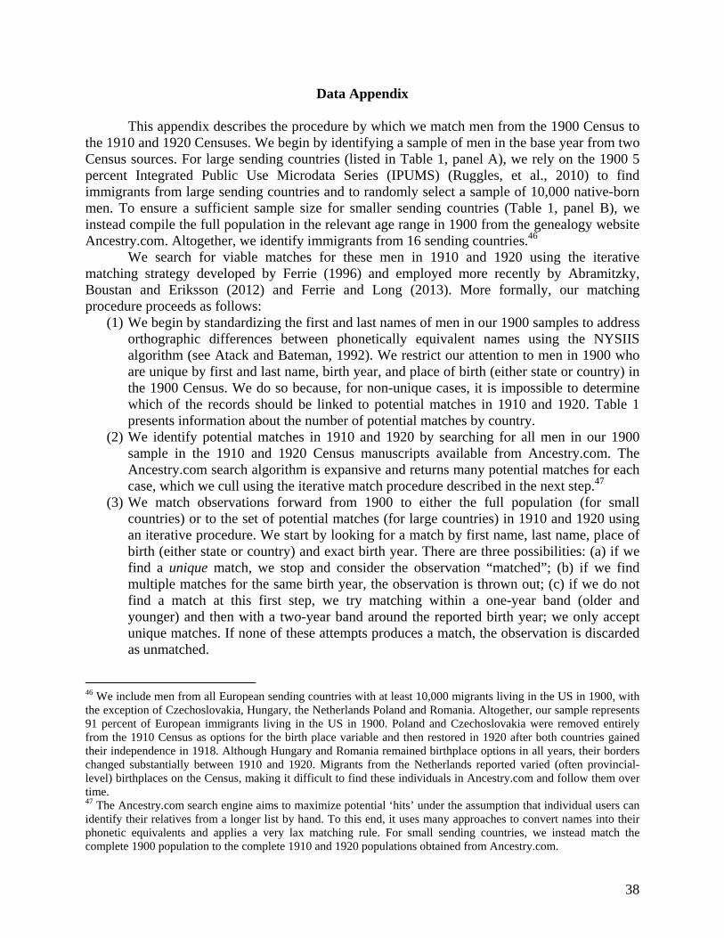
  38

Data Appendix

This appendix describes the procedure by which we match men from the 1900 Census to the 1910 and 1920 Censuses. We begin by identifying a sample of men in the base year from two Census sources. For large sending countries (listed in Table 1, panel A), we rely on the 1900 5 percent Integrated Public Use Microdata Series (IPUMS) (Ruggles, et al., 2010) to find immigrants from large sending countries and to randomly select a sample of 10,000 native-born men. To ensure a sufficient sample size for smaller sending countries (Table 1, panel B), we instead compile the full population in the relevant age range in 1900 from the genealogy website Ancestry.com. Altogether, we identify immigrants from 16 sending countries.46

We search for viable matches for these men in 1910 and 1920 using the iterative matching strategy developed by Ferrie (1996) and employed more recently by Abramitzky, Boustan and Eriksson (2012) and Ferrie and Long (2013). More formally, our matching procedure proceeds as follows:

(1) We begin by standardizing the first and last names of men in our 1900 samples to address orthographic differences between phonetically equivalent names using the NYSIIS algorithm (see Atack and Bateman, 1992). We restrict our attention to men in 1900 who are unique by first and last name, birth year, and place of birth (either state or country) in the 1900 Census. We do so because, for non-unique cases, it is impossible to determine which of the records should be linked to potential matches in 1910 and 1920. Table 1 presents information about the number of potential matches by country.

(2) We identify potential matches in 1910 and 1920 by searching for all men in our 1900 sample in the 1910 and 1920 Census manuscripts available from Ancestry.com. The Ancestry.com search algorithm is expansive and returns many potential matches for each case, which we cull using the iterative match procedure described in the next step.47

(3) We match observations forward from 1900 to either the full population (for small countries) or to the set of potential matches (for large countries) in 1910 and 1920 using an iterative procedure. We start by looking for a match by first name, last name, place of birth (either state or country) and exact birth year. There are three possibilities: (a) if we find a unique match, we stop and consider the observation “matched”; (b) if we find multiple matches for the same birth year, the observation is thrown out; (c) if we do not find a match at this first step, we try matching within a one-year band (older and younger) and then with a two-year band around the reported birth year; we only accept unique matches. If none of these attempts produces a match, the observation is discarded as unmatched.

                                                            46 We include men from all European sending countries with at least 10,000 migrants living in the US in 1900, with the exception of Czechoslovakia, Hungary, the Netherlands Poland and Romania. Altogether, our sample represents 91 percent of European immigrants living in the US in 1900. Poland and Czechoslovakia were removed entirely from the 1910 Census as options for the birth place variable and then restored in 1920 after both countries gained their independence in 1918. Although Hungary and Romania remained birthplace options in all years, their borders changed substantially between 1910 and 1920. Migrants from the Netherlands reported varied (often provincial-level) birthplaces on the Census, making it difficult to find these individuals in Ancestry.com and follow them over time. 47 The Ancestry.com search engine aims to maximize potential ‘hits’ under the assumption that individual users can identify their relatives from a longer list by hand. To this end, it uses many approaches to convert names into their phonetic equivalents and applies a very lax matching rule. For small sending countries, we instead match the complete 1900 population to the complete 1910 and 1920 populations obtained from Ancestry.com.

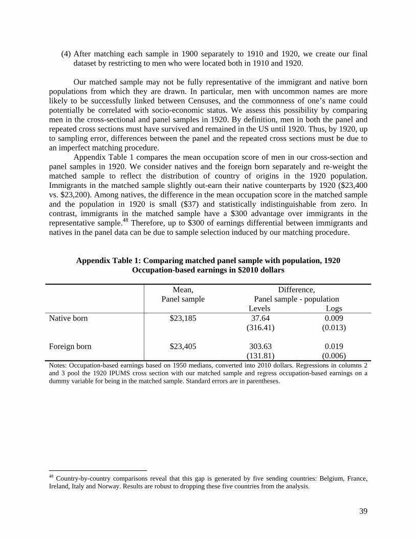
  39

(4) After matching each sample in 1900 separately to 1910 and 1920, we create our final dataset by restricting to men who were located both in 1910 and 1920. Our matched sample may not be fully representative of the immigrant and native born

populations from which they are drawn. In particular, men with uncommon names are more likely to be successfully linked between Censuses, and the commonness of one’s name could potentially be correlated with socio-economic status. We assess this possibility by comparing men in the cross-sectional and panel samples in 1920. By definition, men in both the panel and repeated cross sections must have survived and remained in the US until 1920. Thus, by 1920, up to sampling error, differences between the panel and the repeated cross sections must be due to an imperfect matching procedure.

Appendix Table 1 compares the mean occupation score of men in our cross-section and panel samples in 1920. We consider natives and the foreign born separately and re-weight the matched sample to reflect the distribution of country of origins in the 1920 population. Immigrants in the matched sample slightly out-earn their native counterparts by 1920 ($23,400 vs. $23,200). Among natives, the difference in the mean occupation score in the matched sample and the population in 1920 is small ($37) and statistically indistinguishable from zero. In contrast, immigrants in the matched sample have a $300 advantage over immigrants in the representative sample.48 Therefore, up to $300 of earnings differential between immigrants and natives in the panel data can be due to sample selection induced by our matching procedure.

Appendix Table 1: Comparing matched panel sample with population, 1920 Occupation-based earnings in $2010 dollars

Mean,

Panel sample Difference,

Panel sample - population Levels Logs Native born $23,185 37.64 0.009 (316.41) (0.013) Foreign born $23,405 303.63 0.019 (131.81) (0.006) Notes: Occupation-based earnings based on 1950 medians, converted into 2010 dollars. Regressions in columns 2 and 3 pool the 1920 IPUMS cross section with our matched sample and regress occupation-based earnings on a dummy variable for being in the matched sample. Standard errors are in parentheses.

                                                            48 Country-by-country comparisons reveal that this gap is generated by five sending countries: Belgium, France, Ireland, Italy and Norway. Results are robust to dropping these five countries from the analysis.

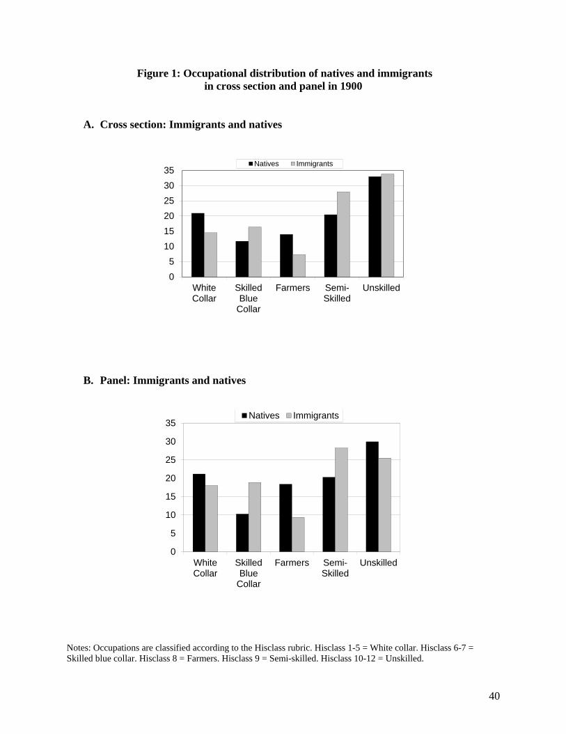
  40

Figure 1: Occupational distribution of natives and immigrants in cross section and panel in 1900

A. Cross section: Immigrants and natives

B. Panel: Immigrants and natives

Notes: Occupations are classified according to the Hisclass rubric. Hisclass 1-5 = White collar. Hisclass 6-7 = Skilled blue collar. Hisclass 8 = Farmers. Hisclass 9 = Semi-skilled. Hisclass 10-12 = Unskilled.

0

5

10

15

20

25

30

35

WhiteCollar

SkilledBlue

Collar

Farmers Semi-Skilled

Unskilled

Natives Immigrants

0

5

10

15

20

25

30

35

WhiteCollar

SkilledBlue

Collar

Farmers Semi-Skilled

Unskilled

Natives Immigrants

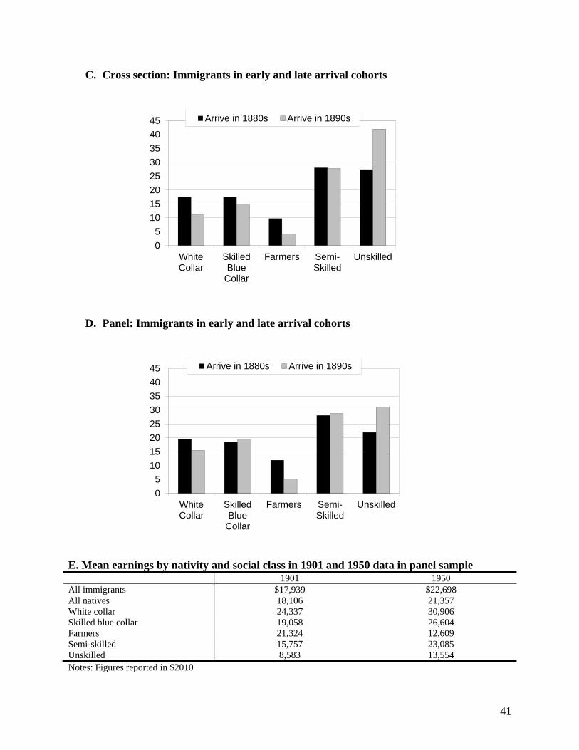
  41

C. Cross section: Immigrants in early and late arrival cohorts

D. Panel: Immigrants in early and late arrival cohorts

E. Mean earnings by nativity and social class in 1901 and 1950 data in panel sample 1901 1950 All immigrants $17,939 $22,698 All natives 18,106 21,357 White collar 24,337 30,906 Skilled blue collar 19,058 26,604 Farmers 21,324 12,609 Semi-skilled 15,757 23,085 Unskilled 8,583 13,554 Notes: Figures reported in $2010

0

5

10

15

20

25

30

35

40

45

WhiteCollar

SkilledBlue

Collar

Farmers Semi-Skilled

Unskilled

Arrive in 1880s Arrive in 1890s

0

5

10

15

20

25

30

35

40

45

WhiteCollar

SkilledBlue

Collar

Farmers Semi-Skilled

Unskilled

Arrive in 1880s Arrive in 1890s

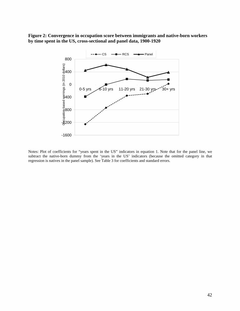
  42

Figure 2: Convergence in occupation score between immigrants and native-born workers by time spent in the US, cross-sectional and panel data, 1900-1920

Notes: Plot of coefficients for “years spent in the US” indicators in equation 1. Note that for the panel line, we subtract the native-born dummy from the ‘years in the US’ indicators (because the omitted category in that regression is natives in the panel sample). See Table 3 for coefficients and standard errors.

-1600

-1200

-800

-400

0

400

800

0-5 yrs 6-10 yrs 11-20 yrs 21-30 yrs 30+ yrs

Occ

upat

ion-

base

d ea

rnin

gs (

in 2

010

dolla

rs)

CS RCS Panel

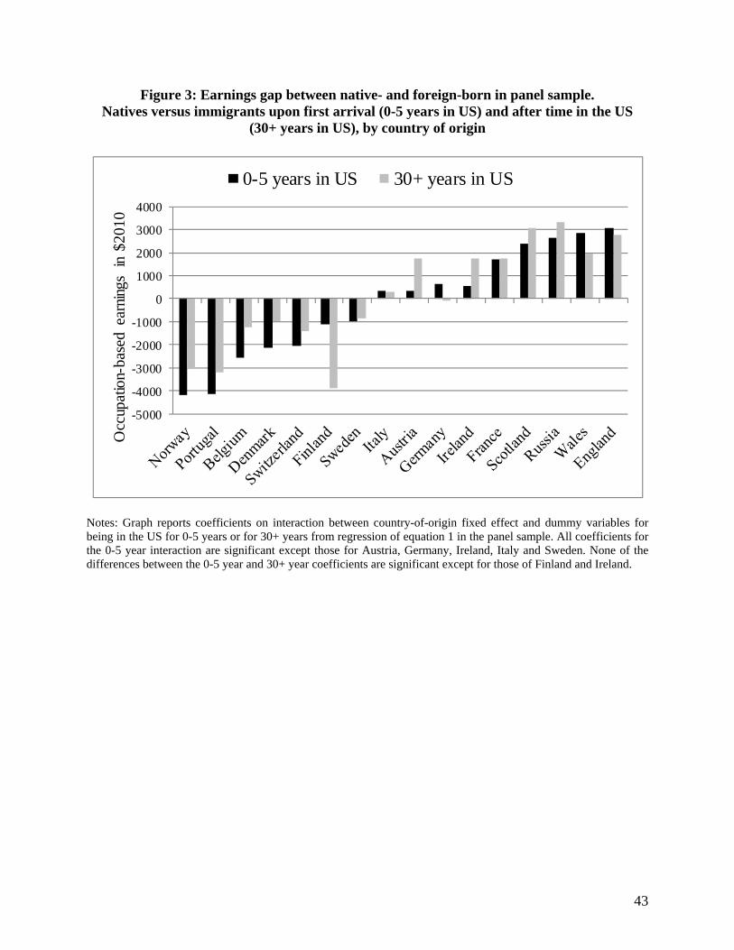
  43

Figure 3: Earnings gap between native- and foreign-born in panel sample. Natives versus immigrants upon first arrival (0-5 years in US) and after time in the US

(30+ years in US), by country of origin  

-5000

-4000

-3000

-2000

-1000

0

1000

2000

3000

4000

Occ

upat

ion-

base

d ea

rnin

gs

in $

2010

0-5 years in US 30+ years in US

Notes: Graph reports coefficients on interaction between country-of-origin fixed effect and dummy variables for being in the US for 0-5 years or for 30+ years from regression of equation 1 in the panel sample. All coefficients for the 0-5 year interaction are significant except those for Austria, Germany, Ireland, Italy and Sweden. None of the differences between the 0-5 year and 30+ year coefficients are significant except for those of Finland and Ireland.

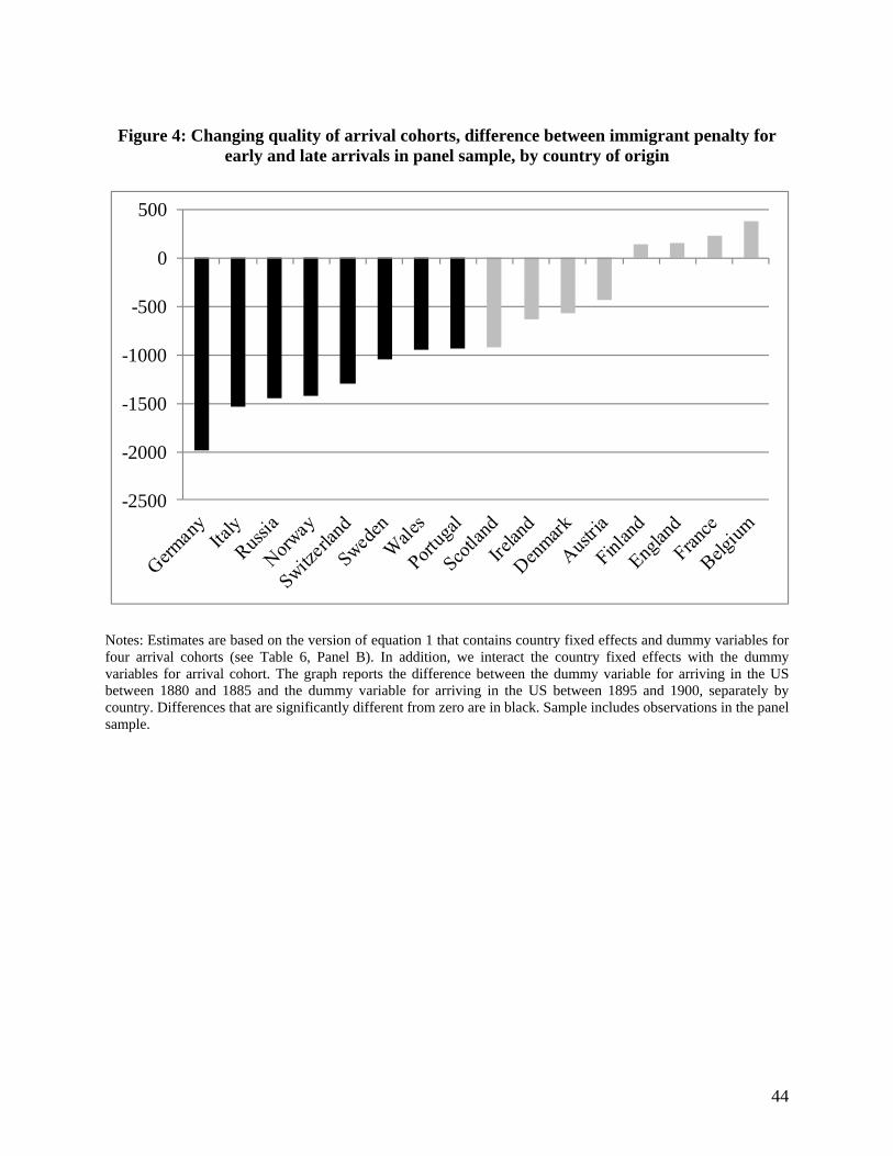
  44

Figure 4: Changing quality of arrival cohorts, difference between immigrant penalty for

early and late arrivals in panel sample, by country of origin

-2500

-2000

-1500

-1000

-500

0

500

Notes: Estimates are based on the version of equation 1 that contains country fixed effects and dummy variables for four arrival cohorts (see Table 6, Panel B). In addition, we interact the country fixed effects with the dummy variables for arrival cohort. The graph reports the difference between the dummy variable for arriving in the US between 1880 and 1885 and the dummy variable for arriving in the US between 1895 and 1900, separately by country. Differences that are significantly different from zero are in black. Sample includes observations in the panel sample.

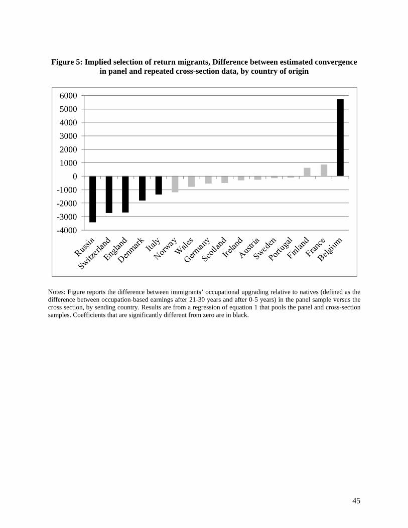
  45

Figure 5: Implied selection of return migrants, Difference between estimated convergence

in panel and repeated cross-section data, by country of origin

-4000

-3000

-2000

-1000

0

1000

2000

3000

4000

5000

6000

Notes: Figure reports the difference between immigrants’ occupational upgrading relative to natives (defined as the difference between occupation-based earnings after 21-30 years and after 0-5 years) in the panel sample versus the cross section, by sending country. Results are from a regression of equation 1 that pools the panel and cross-section samples. Coefficients that are significantly different from zero are in black.

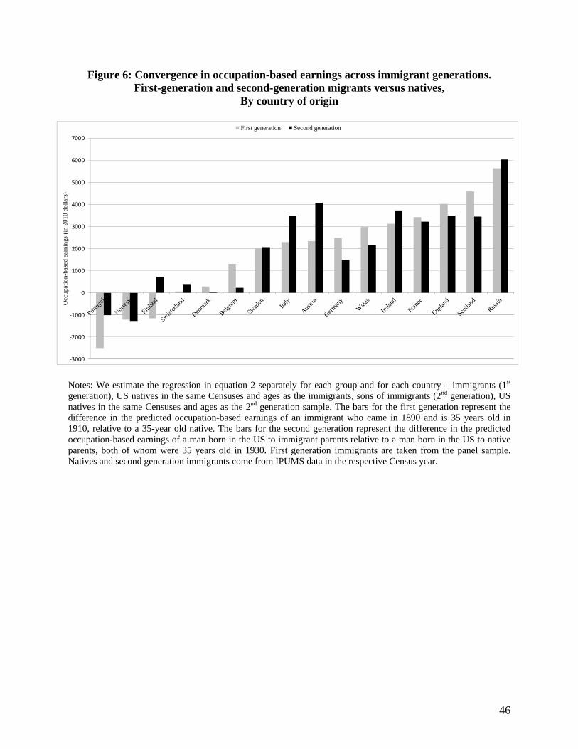
  46

Figure 6: Convergence in occupation-based earnings across immigrant generations. First-generation and second-generation migrants versus natives,

By country of origin

Notes: We estimate the regression in equation 2 separately for each group and for each country – immigrants (1st generation), US natives in the same Censuses and ages as the immigrants, sons of immigrants (2nd generation), US natives in the same Censuses and ages as the 2nd generation sample. The bars for the first generation represent the difference in the predicted occupation-based earnings of an immigrant who came in 1890 and is 35 years old in 1910, relative to a 35-year old native. The bars for the second generation represent the difference in the predicted occupation-based earnings of a man born in the US to immigrant parents relative to a man born in the US to native parents, both of whom were 35 years old in 1930. First generation immigrants are taken from the panel sample. Natives and second generation immigrants come from IPUMS data in the respective Census year.

‐3000

‐2000

‐1000

0

1000

2000

3000

4000

5000

6000

7000

Occ

upat

ion-

base

d ea

rnin

gs (

in 2

010

dolla

rs)

First generation Second generation

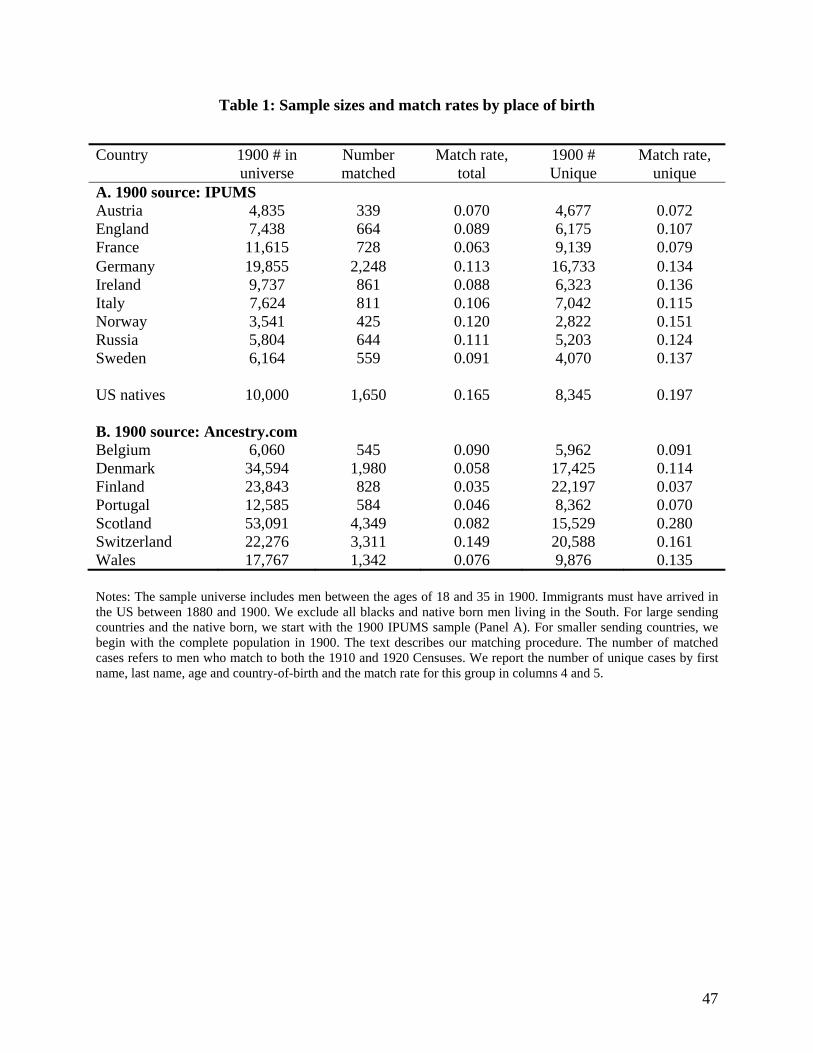
  47

Table 1: Sample sizes and match rates by place of birth

 Notes: The sample universe includes men between the ages of 18 and 35 in 1900. Immigrants must have arrived in the US between 1880 and 1900. We exclude all blacks and native born men living in the South. For large sending countries and the native born, we start with the 1900 IPUMS sample (Panel A). For smaller sending countries, we begin with the complete population in 1900. The text describes our matching procedure. The number of matched cases refers to men who match to both the 1910 and 1920 Censuses. We report the number of unique cases by first name, last name, age and country-of-birth and the match rate for this group in columns 4 and 5.

Country 1900 # in universe

Number matched

Match rate, total

1900 # Unique

Match rate, unique

A. 1900 source: IPUMS Austria 4,835 339 0.070 4,677 0.072 England 7,438 664 0.089 6,175 0.107 France 11,615 728 0.063 9,139 0.079 Germany 19,855 2,248 0.113 16,733 0.134 Ireland 9,737 861 0.088 6,323 0.136 Italy 7,624 811 0.106 7,042 0.115 Norway 3,541 425 0.120 2,822 0.151 Russia 5,804 644 0.111 5,203 0.124 Sweden 6,164 559 0.091 4,070 0.137 US natives 10,000 1,650 0.165 8,345 0.197 B. 1900 source: Ancestry.com Belgium 6,060 545 0.090 5,962 0.091 Denmark 34,594 1,980 0.058 17,425 0.114 Finland 23,843 828 0.035 22,197 0.037 Portugal 12,585 584 0.046 8,362 0.070 Scotland 53,091 4,349 0.082 15,529 0.280 Switzerland 22,276 3,311 0.149 20,588 0.161 Wales 17,767 1,342 0.076 9,876 0.135

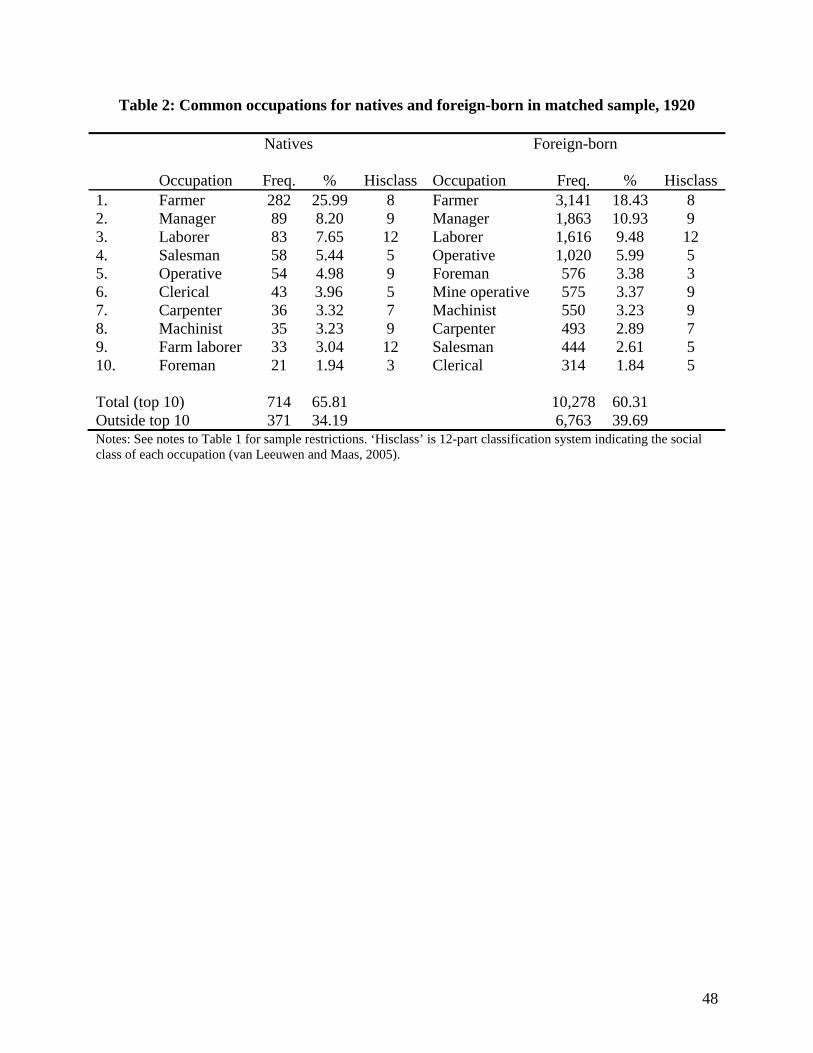
  48

Table 2: Common occupations for natives and foreign-born in matched sample, 1920 Natives

Foreign-born

Occupation Freq. % Hisclass Occupation Freq. % Hisclass1. Farmer 282 25.99 8 Farmer 3,141 18.43 8 2. Manager 89 8.20 9 Manager 1,863 10.93 9 3. Laborer 83 7.65 12 Laborer 1,616 9.48 12 4. Salesman 58 5.44 5 Operative 1,020 5.99 5 5. Operative 54 4.98 9 Foreman 576 3.38 3 6. Clerical 43 3.96 5 Mine operative 575 3.37 9 7. Carpenter 36 3.32 7 Machinist 550 3.23 9 8. Machinist 35 3.23 9 Carpenter 493 2.89 7 9. Farm laborer 33 3.04 12 Salesman 444 2.61 5 10. Foreman 21 1.94 3 Clerical 314 1.84 5 Total (top 10) 714 65.81 10,278 60.31 Outside top 10 371 34.19 6,763 39.69 Notes: See notes to Table 1 for sample restrictions. ‘Hisclass’ is 12-part classification system indicating the social class of each occupation (van Leeuwen and Maas, 2005).

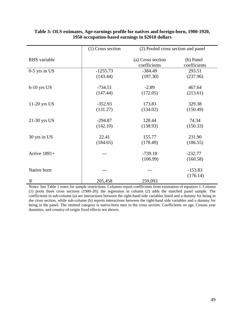
  49

Table 3: OLS estimates, Age-earnings profile for natives and foreign-born, 1900-1920, 1950 occupation-based earnings in $2010 dollars

(1) Cross section

(2) Pooled cross section and panel

RHS variable (a) Cross section coefficients

(b) Panel coefficients

0-5 yrs in US -1255.73 -384.49 293.51 (143.44) (187.30) (237.96) 6-10 yrs US -734.51 -2.89 467.64 (147.44) (172.05) (213.61) 11-20 yrs US -352.93 173.83 329.38 (131.27) (134.02) (150.49) 21-30 yrs US -294.87 128.44 74.34 (142.10) (138.93) (150.33) 30 yrs in US 22.41 155.77 231.90 (184.65) (178.49) (186.55) Arrive 1891+ --- -739.18 -232.77 (106.99) (160.58) Native born --- --- -153.83 (176.14) N 205,458 259,093 Notes: See Table 1 notes for sample restrictions. Columns report coefficients from estimation of equation 1. Column (1) pools three cross sections (1900-20); the regression in column (2) adds the matched panel sample. The coefficients in sub-column (a) are interactions between the right-hand side variables listed and a dummy for being in the cross section, while sub-column (b) reports interactions between the right-hand side variables and a dummy for being in the panel. The omitted category is native-born men in the cross section. Coefficients on age, Census year dummies, and country-of-origin fixed effects not shown.

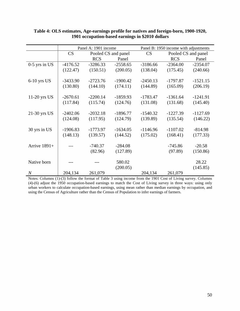
  50

Table 4: OLS estimates, Age-earnings profile for natives and foreign-born, 1900-1920, 1901 occupation-based earnings in $2010 dollars

Panel A: 1901 income Panel B: 1950 income with adjustments CS Pooled CS and panel CS Pooled CS and panel RCS Panel RCS Panel 0-5 yrs in US -4176.52 -3286.33 -2558.65 -3186.66 -2364.00 -2354.07 (122.47) (150.51) (200.05) (138.04) (175.45) (240.66) 6-10 yrs US -3433.90 -2723.76 -1900.42 -2450.13 -1797.87 -1521.15 (130.80) (144.10) (174.11) (144.89) (165.09) (206.19) 11-20 yrs US -2670.61 -2200.14 -1859.93 -1783.47 -1361.64 -1241.91 (117.84) (115.74) (124.76) (131.08) (131.68) (145.40) 21-30 yrs US -2402.06 -2032.18 -1896.77 -1540.32 -1227.39 -1127.69 (124.08) (117.95) (124.79) (139.89) (135.54) (146.22) 30 yrs in US -1906.83 -1773.97 -1634.05 -1146.96 -1107.02 -814.98 (148.13) (139.57) (144.52) (175.02) (168.41) (177.33) Arrive 1891+ --- -740.37 -284.08 -745.86 -20.58 (82.96) (127.89) (97.89) (150.86) Native born --- --- 580.02 28.22 (200.05) (145.85) N 204,134 261,079 204,134 261,079 Notes: Columns (1)-(3) follow the format of Table 3 using income from the 1901 Cost of Living survey. Columns (4)-(6) adjust the 1950 occupation-based earnings to match the Cost of Living survey in three ways: using only urban workers to calculate occupation-based earnings, using mean rather than median earnings by occupation, and using the Census of Agriculture rather than the Census of Population to infer earnings of farmers.

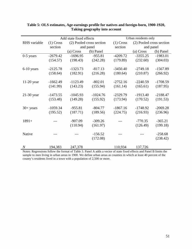
  51

Table 5: OLS estimates, Age-earnings profile for natives and foreign-born, 1900-1920, Taking geography into account

Add state fixed effects Urban residents only RHS variable (1) Cross

section (2) Pooled cross section

and panel (1) Cross section

(2) Pooled cross section and panel

(a) Cross (b) Panel (a) Cross (b) Panel 0-5 years -2679.42 -1696.95 -955.81 -4209.72 -3355.25 -1983.01 (154.57) (198.43) (242.28) (179.89) (232.60) (304.03) 6-10 years -2125.78 -1323.73 -817.13 -3450.40 -2749.18 -1567.89 (158.64) (182.91) (216.28) (180.64) (210.87) (266.92) 11-20 year -1662.49 -1123.49 -802.01 -2752.16 -2240.59 -1708.59 (141.99) (143.23) (155.94) (161.14) (165.61) (187.95) 21-30 year -1473.55 -1045.93 -1024.76 -2329.79 -1913.40 -2188.47 (153.48) (149.28) (155.92) (173.94) (170.52) (191.53) 30+ years -1059.34 -955.81 -804.77 -1867.16 -1748.92 -2069.28

(195.52) (187.71) (189.56) (224.75) (216.93) (236.96)

1891+ --- -907.09 -309.26 --- -770.35 -365.21 (110.94) (161.97) (126.49) (199.18)

Native --- --- -156.52 --- --- -258.68 (172.08) (238.42) N 194,383 247,378 110,934 137,726 Notes: Regressions follow the format of Table 3. Panel A adds a vector of state fixed effects and Panel B limits the sample to men living in urban areas in 1900. We define urban areas as counties in which at least 40 percent of the county’s residents lived in a town with a population of 2,500 or more.

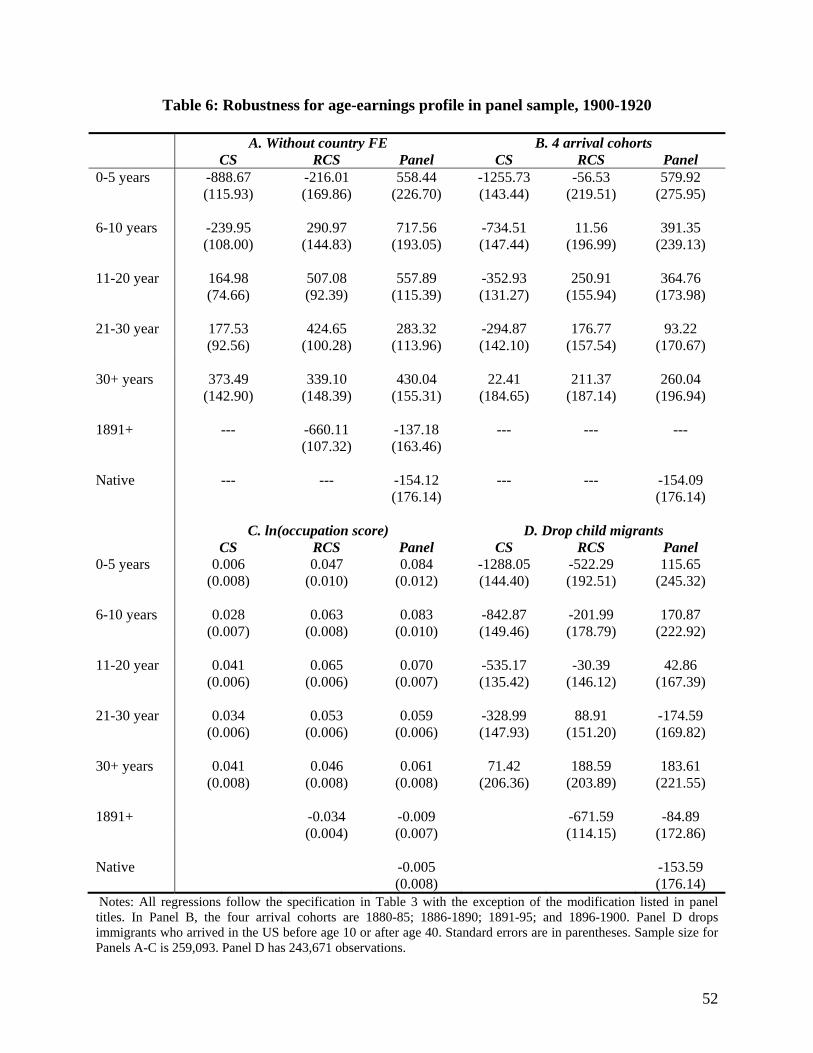
  52

Table 6: Robustness for age-earnings profile in panel sample, 1900-1920 A. Without country FE B. 4 arrival cohorts CS RCS Panel CS RCS Panel 0-5 years -888.67 -216.01 558.44 -1255.73 -56.53 579.92 (115.93) (169.86) (226.70) (143.44) (219.51) (275.95) 6-10 years -239.95 290.97 717.56 -734.51 11.56 391.35 (108.00) (144.83) (193.05) (147.44) (196.99) (239.13) 11-20 year 164.98 507.08 557.89 -352.93 250.91 364.76 (74.66) (92.39) (115.39) (131.27) (155.94) (173.98) 21-30 year 177.53 424.65 283.32 -294.87 176.77 93.22 (92.56) (100.28) (113.96) (142.10) (157.54) (170.67) 30+ years 373.49 339.10 430.04 22.41 211.37 260.04 (142.90) (148.39) (155.31) (184.65) (187.14) (196.94) 1891+ --- -660.11 -137.18 --- --- --- (107.32) (163.46) Native --- --- -154.12 --- --- -154.09 (176.14) (176.14) C. ln(occupation score) D. Drop child migrants CS RCS Panel CS RCS Panel 0-5 years 0.006 0.047 0.084 -1288.05 -522.29 115.65 (0.008) (0.010) (0.012) (144.40) (192.51) (245.32) 6-10 years 0.028 0.063 0.083 -842.87 -201.99 170.87 (0.007) (0.008) (0.010) (149.46) (178.79) (222.92) 11-20 year 0.041 0.065 0.070 -535.17 -30.39 42.86 (0.006) (0.006) (0.007) (135.42) (146.12) (167.39) 21-30 year 0.034 0.053 0.059 -328.99 88.91 -174.59 (0.006) (0.006) (0.006) (147.93) (151.20) (169.82) 30+ years 0.041 0.046 0.061 71.42 188.59 183.61

(0.008) (0.008) (0.008) (206.36) (203.89) (221.55)

1891+ -0.034 -0.009 -671.59 -84.89 (0.004) (0.007) (114.15) (172.86)

Native -0.005 -153.59 (0.008) (176.14)

Notes: All regressions follow the specification in Table 3 with the exception of the modification listed in panel titles. In Panel B, the four arrival cohorts are 1880-85; 1886-1890; 1891-95; and 1896-1900. Panel D drops immigrants who arrived in the US before age 10 or after age 40. Standard errors are in parentheses. Sample size for Panels A-C is 259,093. Panel D has 243,671 observations.

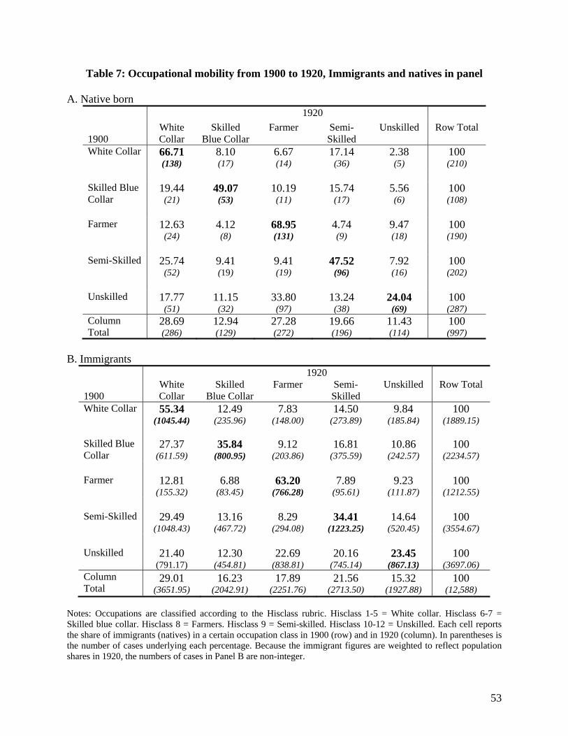
  53

Table 7: Occupational mobility from 1900 to 1920, Immigrants and natives in panel

A. Native born

B. Immigrants

1920 1900

White Collar

Skilled Blue Collar

Farmer Semi-Skilled

Unskilled Row Total

White Collar 55.34 (1045.44)

12.49 (235.96)

7.83 (148.00)

14.50 (273.89)

9.84 (185.84)

100 (1889.15)

Skilled Blue Collar

27.37 (611.59)

35.84 (800.95)

9.12 (203.86)

16.81 (375.59)

10.86 (242.57)

100 (2234.57)

Farmer 12.81

(155.32) 6.88

(83.45)63.20

(766.28)7.89

(95.61)9.23

(111.87) 100

(1212.55) Semi-Skilled 29.49

(1048.43) 13.16

(467.72)8.29

(294.08)34.41

(1223.25)14.64

(520.45) 100

(3554.67) Unskilled 21.40

(791.17) 12.30

(454.81)22.69

(838.81)20.16

(745.14)23.45

(867.13) 100

(3697.06)Column Total

29.01 (3651.95)

16.23 (2042.91)

17.89 (2251.76)

21.56 (2713.50)

15.32 (1927.88)

100 (12,588)

Notes: Occupations are classified according to the Hisclass rubric. Hisclass 1-5 = White collar. Hisclass 6-7 = Skilled blue collar. Hisclass 8 = Farmers. Hisclass 9 = Semi-skilled. Hisclass 10-12 = Unskilled. Each cell reports the share of immigrants (natives) in a certain occupation class in 1900 (row) and in 1920 (column). In parentheses is the number of cases underlying each percentage. Because the immigrant figures are weighted to reflect population shares in 1920, the numbers of cases in Panel B are non-integer.

1920

1900

White Collar

Skilled Blue Collar

Farmer Semi-Skilled

Unskilled Row Total

White Collar 66.71 (138)

8.10 (17)

6.67 (14)

17.14 (36)

2.38 (5)

100 (210)

Skilled Blue Collar

19.44 (21)

49.07 (53)

10.19 (11)

15.74 (17)

5.56 (6)

100 (108)

Farmer 12.63

(24) 4.12 (8)

68.95 (131)

4.74 (9)

9.47 (18)

100 (190)

Semi-Skilled 25.74

(52) 9.41 (19)

9.41 (19)

47.52 (96)

7.92 (16)

100 (202)

Unskilled 17.77

(51) 11.15

(32)33.80

(97)13.24

(38)24.04

(69) 100 (287)

Column Total

28.69 (286)

12.94 (129)

27.28 (272)

19.66 (196)

11.43 (114)

100 (997)