Embed Size (px)
Citation preview
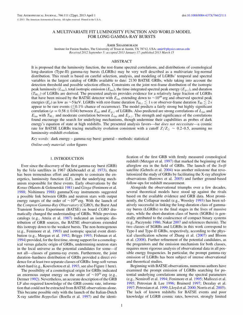
The Astrophysical Journal, 766:111 (22pp), 2013 April 1 doi:10.1088/0004-637X/766/2/111C© 2013. The American Astronomical Society. All rights reserved. Printed in the U.S.A.
A MULTIVARIATE FIT LUMINOSITY FUNCTION AND WORLD MODELFOR LONG GAMMA-RAY BURSTS
Amir ShahmoradiInstitute for Fusion Studies, The University of Texas at Austin, TX 78712, USA; [email protected]
Received 2012 September 5; accepted 2013 January 17; published 2013 March 15
ABSTRACT
It is proposed that the luminosity function, the rest-frame spectral correlations, and distributions of cosmologicallong-duration (Type-II) gamma-ray bursts (LGRBs) may be very well described as a multivariate log-normaldistribution. This result is based on careful selection, analysis, and modeling of LGRBs’ temporal and spectralvariables in the largest catalog of GRBs available to date: 2130 BATSE GRBs, while taking into account thedetection threshold and possible selection effects. Constraints on the joint rest-frame distribution of the isotropicpeak luminosity (Liso), total isotropic emission (Eiso), the time-integrated spectral peak energy (Ep,z), and duration(T90,z) of LGRBs are derived. The presented analysis provides evidence for a relatively large fraction of LGRBsthat have been missed by the BATSE detector with Eiso extending down to ∼1049 erg and observed spectral peakenergies (Ep) as low as ∼5 keV. LGRBs with rest-frame duration T90,z � 1 s or observer-frame duration T90 � 2 sappear to be rare events (�0.1% chance of occurrence). The model predicts a fairly strong but highly significantcorrelation (ρ = 0.58 ± 0.04) between Eiso and Ep,z of LGRBs. Also predicted are strong correlations of Liso andEiso with T90,z and moderate correlation between Liso and Ep,z. The strength and significance of the correlationsfound encourage the search for underlying mechanisms, though undermine their capabilities as probes of darkenergy’s equation of state at high redshifts. The presented analysis favors—but does not necessitate—a cosmicrate for BATSE LGRBs tracing metallicity evolution consistent with a cutoff Z/Z� ∼ 0.2–0.5, assuming noluminosity–redshift evolution.
Key words: dark energy – gamma-ray burst: general – methods: statistical
Online-only material: color figures
1. INTRODUCTION
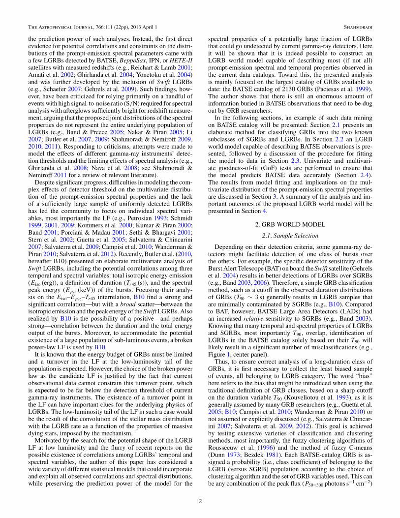
Ever since the discovery of the first gamma-ray burst (GRB)by the Vela satellites in 1967 (Klebesadel et al. 1973), therehas been tremendous effort and attempts to constrain the en-ergetics, luminosity function (LF), and the underlying mech-anism responsible for these events. Early observations by theKonus (Mazets & Golenetskii 1981) and Ginga (Fenimore et al.1988; Nishimura 1988) gamma/X-ray instruments suggesteda possible link between GRBs and neutron stars with outputenergy ranges of the order of ∼1040 erg. With the launch ofthe Compton Gamma-Ray Observatory (CGRO), the Burst AndTransient Source Experiment (BATSE) on board CGRO dra-matically changed the understanding of GRBs. While previouscatalogs (e.g., Atteia et al. 1987) indicated an isotropic dis-tribution of GRB sources, the BATSE observations extendedthis isotropy down to the weakest bursts. The non-homogenous(e.g., Fenimore et al. 1993) and isotropic spacial event distri-bution (e.g., Meegan et al. 1992; Briggs 1993; Fishman et al.1994) provided, for the first time, strong support for a cosmolog-ical versus galactic origin of GRBs, undermining neutron starsin the local universe as the potential candidates for some—ifnot all—classes of gamma-ray events. Furthermore, the jointduration–hardness distribution of GRBs provided a direct evi-dence for at least two separate classes of GRBs: long-soft versusshort-hard (e.g., Kouveliotou et al. 1993, see also Figure 1 here).
The possibility of a cosmological origin for GRBs indicatedan enormous output energy on the order of ∼1051 erg (e.g.,Dermer 1992). Nevertheless, an accurate description of the GRBLF also required knowledge of the GRB cosmic rate, informa-tion that could not be extracted from BATSE observations alone.This became possible only with the launch of the Italian-DutchX-ray satellite BeppoSax (Boella et al. 1997) and the identi-
fication of the first GRB with firmly measured cosmologicalredshift (Metzger et al. 1997) that marked the beginning of theafterglow era in the field of GRBs. The launch of the Swiftsatellite (Gehrels et al. 2004) was another milestone that revo-lutionized the study of GRBs by facilitating the X-ray afterglowobservations (Burrows et al. 2005) and further ground-basedfollow-ups for redshift measurement.
Alongside the observational triumphs over a few decades,several theoretical models have stood up against the rivalsbased on the available evidence and GRB data. Most promi-nently, the Collapsar model (e.g., Woosley 1993) has been rel-atively successful in linking the long-duration class of gamma-ray bursts (LGRBs) to the final stages in the lives of massivestars, while the short-duration class of bursts (SGRBs) is gen-erally attributed to the coalescence of compact binary systems(e.g., Paczynski 1986; Nakar 2007 and references therein). Thetwo classes of SGRBs and LGRBs in this work correspond toType-I and Type-II GRBs, respectively, according to the phys-ical classification scheme of Zhang et al. (2007) and Bloomet al. (2008). Further refinement of the potential candidates, asthe progenitors and the emission mechanism for both classes,requires more rigorous analysis of observational data in all pos-sible energy frequencies. In particular, the prompt gamma-rayemission of LGRBs has been subject of intense observationaland theoretical studies.
Beginning with BATSE observations, numerous authors haveexamined the prompt emission of LGRBs searching for po-tential underlying correlations among the spectral parameters(e.g., Nemiroff et al. 1994; Fenimore et al. 1995; Mallozzi et al.1995; Petrosian & Lee 1996; Brainerd 1997; Dezalay et al.1997; Petrosian et al. 1999; Lloyd et al. 2000; Norris et al. 2005).The lack of known redshifts for BATSE events and poorknowledge of LGRB cosmic rates, however, strongly limited
1
The Astrophysical Journal, 766:111 (22pp), 2013 April 1 Shahmoradi
the prediction power of such analyses. Instead, the first directevidence for potential correlations and constraints on the distri-butions of the prompt-emission spectral parameters came witha few LGRBs detected by BATSE, BeppoSax, IPN, or HETE-IIsatellites with measured redshifts (e.g., Reichart & Lamb 2001;Amati et al. 2002; Ghirlanda et al. 2004; Yonetoku et al. 2004)and was further developed by the inclusion of Swift LGRBs(e.g., Schaefer 2007; Gehrels et al. 2009). Such findings, how-ever, have been criticized for relying primarily on a handful ofevents with high signal-to-noise ratio (S/N) required for spectralanalysis with afterglows sufficiently bright for redshift measure-ment, arguing that the proposed joint distributions of the spectralproperties do not represent the entire underlying population ofLGRBs (e.g., Band & Preece 2005; Nakar & Piran 2005; Li2007; Butler et al. 2007, 2009; Shahmoradi & Nemiroff 2009,2010, 2011). Responding to criticisms, attempts were made tomodel the effects of different gamma-ray instruments’ detec-tion thresholds and the limiting effects of spectral analysis (e.g.,Ghirlanda et al. 2008; Nava et al. 2008; see Shahmoradi &Nemiroff 2011 for a review of relevant literature).
Despite significant progress, difficulties in modeling the com-plex effects of detector threshold on the multivariate distribu-tion of the prompt-emission spectral properties and the lackof a sufficiently large sample of uniformly detected LGRBshas led the community to focus on individual spectral vari-ables, most importantly the LF (e.g., Petrosian 1993; Schmidt1999, 2001, 2009; Kommers et al. 2000; Kumar & Piran 2000;Band 2001; Porciani & Madau 2001; Sethi & Bhargavi 2001;Stern et al. 2002; Guetta et al. 2005; Salvaterra & Chincarini2007; Salvaterra et al. 2009; Campisi et al. 2010; Wanderman &Piran 2010; Salvaterra et al. 2012). Recently, Butler et al. (2010,hereafter B10) presented an elaborate multivariate analysis ofSwift LGRBs, including the potential correlations among threetemporal and spectral variables: total isotropic energy emission(Eiso (erg)), a definition of duration (Tr45 (s)), and the spectralpeak energy (Ep,z (keV)) of the bursts. Focusing their analy-sis on the Eiso–Ep,z–Tr45 interrelation, B10 find a strong andsignificant correlation—but with a broad scatter—between theisotropic emission and the peak energy of the Swift LGRBs. Alsorealized by B10 is the possibility of a positive—and perhapsstrong—correlation between the duration and the total energyoutput of the bursts. Moreover, to accommodate the potentialexistence of a large population of sub-luminous events, a brokenpower-law LF is used by B10.
It is known that the energy budget of GRBs must be limitedand a turnover in the LF at the low-luminosity tail of thepopulation is expected. However, the choice of the broken powerlaw as the candidate LF is justified by the fact that currentobservational data cannot constrain this turnover point, whichis expected to be far below the detection threshold of currentgamma-ray instruments. The existence of a turnover point inthe LF can have important clues for the underlying physics ofLGRBs. The low-luminosity tail of the LF in such a case wouldbe the result of the convolution of the stellar mass distributionwith the LGRB rate as a function of the properties of massivedying stars, imposed by the mechanism.
Motivated by the search for the potential shape of the LGRBLF at low luminosity and the flurry of recent reports on thepossible existence of correlations among LGRBs’ temporal andspectral variables, the author of this paper has considered awide variety of different statistical models that could incorporateand explain all observed correlations and spectral distributions,while preserving the prediction power of the model for the
spectral properties of a potentially large fraction of LGRBsthat could go undetected by current gamma-ray detectors. Hereit will be shown that it is indeed possible to construct anLGRB world model capable of describing most (if not all)prompt-emission spectral and temporal properties observed inthe current data catalogs. Toward this, the presented analysisis mainly focused on the largest catalog of GRBs available todate: the BATSE catalog of 2130 GRBs (Paciesas et al. 1999).The author shows that there is still an enormous amount ofinformation buried in BATSE observations that need to be dugout by GRB researchers.
In the following sections, an example of such data miningon BATSE catalog will be presented: Section 2.1 presents anelaborate method for classifying GRBs into the two knownsubclasses of SGRBs and LGRBs. In Section 2.2 an LGRBworld model capable of describing BATSE observations is pre-sented, followed by a discussion of the procedure for fittingthe model to data in Section 2.3. Univariate and multivari-ate goodness-of-fit (GoF) tests are performed to ensure thatthe model predicts BATSE data accurately (Section 2.4).The results from model fitting and implications on the mul-tivariate distribution of the prompt-emission spectral propertiesare discussed in Section 3. A summary of the analysis and im-portant outcomes of the proposed LGRB world model will bepresented in Section 4.
2. GRB WORLD MODEL
2.1. Sample Selection
Depending on their detection criteria, some gamma-ray de-tectors might facilitate detection of one class of bursts overthe others. For example, the specific detector sensitivity of theBurst Alert Telescope (BAT) on board the Swift satellite (Gehrelset al. 2004) results in better detections of LGRBs over SGRBs(e.g., Band 2003, 2006). Therefore, a simple GRB classificationmethod, such as a cutoff in the observed duration distributionsof GRBs (T90 ∼ 3 s) generally results in LGRB samples thatare minimally contaminated by SGRBs (e.g., B10). Comparedto BAT, however, BATSE Large Area Detectors (LADs) hadan increased relative sensitivity to SGRBs (e.g., Band 2003).Knowing that many temporal and spectral properties of LGRBsand SGRBs, most importantly T90, overlap, identification ofLGRBs in the BATSE catalog solely based on their T90 willlikely result in a significant number of misclassifications (e.g.,Figure 1, center panel).
Thus, to ensure correct analysis of a long-duration class ofGRBs, it is first necessary to collect the least biased sampleof events, all belonging to LGRB category. The word “bias”here refers to the bias that might be introduced when using thetraditional definition of GRB classes, based on a sharp cutoffon the duration variable T90 (Kouveliotou et al. 1993), as it isgenerally assumed by many GRB researchers (e.g., Guetta et al.2005; B10; Campisi et al. 2010; Wanderman & Piran 2010) ornot assumed or explicitly discussed (e.g., Salvaterra & Chincar-ini 2007; Salvaterra et al. 2009, 2012). This goal is achievedby testing extensive varieties of classification and clusteringmethods, most importantly, the fuzzy clustering algorithms ofRousseeuw et al. (1996) and the method of fuzzy C-means(Dunn 1973; Bezdek 1981). Each BATSE-catalog GRB is as-signed a probability (i.e., class coefficient) of belonging to theLGRB (versus SGRB) population according to the choice ofclustering algorithm and the set of GRB variables used. This canbe any combination of the peak flux (P50–300 photons s−1 cm−2)
2
The Astrophysical Journal, 766:111 (22pp), 2013 April 1 Shahmoradi
0.01 0.1 1 10 100 1000
10
100
1000
10000
1366 BATSE LGRBs 600 BATSE SGRBs
Obs
erve
d P
eak
Ene
rgy:
Ep
[keV
]
Observed Duration: T90 [s]
average 1σuncertainty
-2.0 -1.5 -1.0 -0.5 0.0 0.5 1.0 1.5 2.0 2.5 3.00
20
40
60
80
100
120
140
1966 BATSE GRBs 1366 BATSE LGRBs 600 BATSE SGRBs
Cou
nt
Observed Duration: log (T90 [s])
1.0 1.5 2.0 2.5 3.0 3.5 4.00
25
50
75
100
125
150
175
200
225
1966 BATSE GRBs 1366 BATSE LGRBs 600 BATSE SGRBs
Cou
nt
Observed Peak Energy: log (Ep [keV])
Figure 1. Classification of 1966 BATSE LGRBs according to the most suitableclustering algorithm and set of GRB variables (Section 2.1): fuzzy C-meansclassification on Ep and T90. Red and blue colors represent LGRB and SGRBclasses, respectively, in all three plots. Top: the joint T90–Ep distribution. Theuncertainties in LGRBs are derived from the empirical Bayes model discussedin Appendix C. Center: T90 distribution. Bottom: Ep distribution. Ep estimatesare taken from Shahmoradi & Nemiroff (2010). Compare this plot to the plotof Figure 13 of Shahmoradi & Nemiroff (2010), where the entire univariateEp distributions of BATSE GRBs were fit by a two-component Gaussianmixture.
(A color version of this figure is available in the online journal.)
in the BATSE detection energy range, in three differ-ent timescales: 64, 256, and 1024 ms; bolometric fluence(Sbol(erg cm−2)); the spectral peak energy (Ep (keV)) esti-mates by Shahmoradi & Nemiroff (2010); duration (T90 (s));and the fluence-to-peak-flux ratio (FPR (s)). Then GRBs withLGRB class coefficient >0.5 are flagged as long-duration classbursts. Overall, the fuzzy C-means classification method withthe two GRB variables Ep and T90 is preferred over other clus-tering methods and sets of GRB variables (cf. Appendix A).This leads to the selection of 1376 events as LGRBs out ofthe 1966 BATSE GRBs having measured temporal and spectralparameters mentioned above.1
As a further safety check to ensure minimal contaminationof the sample by SGRBs, the light curves of 291 bursts among1966 BATSE GRBs with LGRB class coefficients in the range of0.3–0.7 are visually inspected in the four main energy channelsof BATSE LADs. This leads to reclassification of 17 events(originally flagged as LGRB by the clustering algorithm) topotentially SGRB or soft gamma repeater (SGR) events, andreclassification of seven events (originally flagged as SGRB bythe clustering algorithm) to LGRBs. The result is a reductionin the size of the original LGRB sample from 1376 to 1366(Table 1). It is notable that the inclusion of the uncertaintieson the two GRB variables T90 and Ep turns out to not havesignificant effects on the derived samples of the two GRB classesdiscussed above. Also, a classification based on T50 instead ofT90 results in about the same samples for the two GRB classeswith only a negligible difference of ∼0.7%.
2.2. Model Construction
The goal of the presented analysis is to derive a multivariatemodel that is capable of reproducing the observational data ofthe 1366 BATSE LGRBs. Examples of multivariate treatmentof LGRB data are rare in GRB literature, with the most recent(and perhaps the only) example of such work presented byB10. Conversely, many authors have focused primarily onthe univariate distribution of the spectral parameters, mostimportantly on the LF. A variety of univariate models have beenproposed as the LGRB LF and fit to data by approximatingthe complex detector threshold as a step function (Schmidt1999) or an efficiency grid (e.g., the four-interval efficiencymodeling of Guetta et al. 2005) or by other approximationmethods. A more accurate modeling of the LF, however, requiresat least two LGRB observables incorporated in the model: thebolometric peak flux (Pbol) and the observed peak energy (Ep).The parameter Ep is required, since most gamma-ray detectorsare photon counters, a quantity that depends on not only Pbolbut also Ep of the burst. This leads to the requirement of usinga bivariate distribution as the minimum acceptable model tobegin with, for the purpose of constraining the LF. The choiceof model can be almost anything (e.g., Kommers et al. 2000;Porciani & Madau 2001; Sethi & Bhargavi 2001; Schmidt 2009;Campisi et al. 2010; Wang & Dai 2011), since current theoriesof LGRB prompt emission do not set strong limits on the shapeand range of the LF or any other LGRB spectral or temporalvariables.
1 Data for 1966 BATSE GRBs with firmly measured peak flux, fluence, andduration are taken from The BATSE Gamma Ray Burst Catalogs:http://www.batse.msfc.nasa.gov/batse/grb/catalog/. The spectral peak energy(Ep) estimates of these events are taken from Shahmoradi & Nemiroff (2010),also available for download at https://sites.google.com/site/amshportal/research/aca/in-the-news/lgrb-world-model.
3

The Astrophysical Journal, 766:111 (22pp), 2013 April 1 Shahmoradi
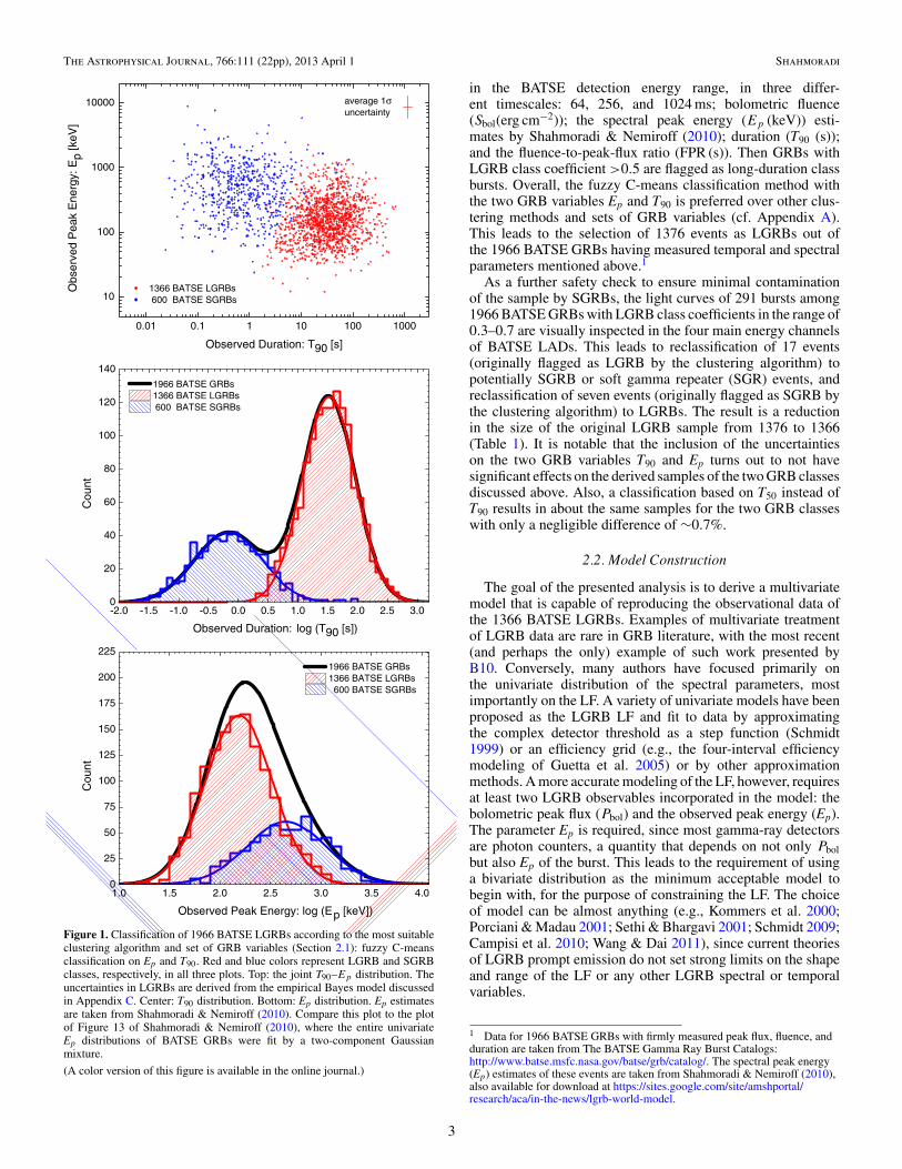
Table 11366 BATSE Catalog Triggers Classified as LGRBs
Trigger Trigger Trigger Trigger Trigger Trigger Trigger Trigger Trigger Trigger Trigger Trigger Trigger Trigger
105 107 109 110 111 114 121 130 133 143 148 160 171 179204 211 214 219 222 223 226 228 235 237 249 257 288 332351 394 398 401 404 408 414 451 465 467 469 472 473 493501 516 526 540 543 548 549 559 563 577 591 594 606 630647 658 659 660 673 676 678 680 685 686 690 692 704 717741 752 753 755 761 764 773 795 803 815 816 820 824 825829 840 841 869 907 914 927 938 946 973 999 1009 1036 10391042 1046 1085 1086 1087 1114 1120 1122 1123 1125 1126 1141 1145 11481150 1152 1153 1156 1157 1159 1167 1190 1192 1196 1197 1200 1204 12131218 1221 1235 1244 1279 1288 1291 1298 1303 1306 1318 1382 1384 13851390 1396 1406 1416 1419 1425 1432 1439 1440 1446 1447 1449 1452 14561458 1467 1468 1472 1492 1515 1533 1540 1541 1551 1552 1558 1559 15611567 1574 1578 1579 1580 1586 1590 1601 1604 1606 1609 1611 1614 16231625 1626 1628 1642 1646 1651 1652 1653 1655 1656 1657 1660 1661 16631664 1667 1676 1687 1693 1700 1701 1704 1711 1712 1714 1717 1730 17311733 1734 1740 1742 1806 1807 1815 1819 1830 1883 1885 1886 1922 19241956 1967 1974 1982 1989 1993 1997 2018 2019 2035 2047 2053 2061 20672069 2070 2074 2077 2079 2080 2081 2083 2087 2090 2093 2101 2102 21052106 2110 2111 2112 2114 2119 2122 2123 2129 2133 2138 2140 2143 21482149 2151 2152 2156 2181 2187 2188 2189 2190 2191 2193 2197 2202 22032204 2207 2211 2213 2219 2228 2230 2232 2233 2240 2244 2252 2253 22542267 2276 2277 2287 2298 2304 2306 2309 2310 2311 2315 2316 2321 23242325 2328 2329 2340 2344 2345 2346 2347 2349 2362 2367 2371 2373 23752380 2381 2383 2385 2387 2391 2392 2393 2394 2405 2419 2423 2428 24292430 2432 2435 2436 2437 2438 2440 2441 2442 2443 2446 2447 2450 24512452 2453 2458 2460 2472 2476 2477 2482 2484 2495 2496 2500 2505 25082510 2511 2515 2519 2522 2528 2530 2533 2537 2541 2551 2560 2569 25702581 2586 2589 2593 2600 2603 2606 2608 2610 2611 2619 2620 2628 26342636 2640 2641 2660 2662 2663 2664 2665 2671 2677 2681 2688 2691 26952696 2697 2700 2703 2706 2709 2711 2719 2725 2727 2736 2749 2750 27512753 2767 2770 2774 2775 2780 2790 2793 2797 2798 2812 2815 2825 28302831 2843 2848 2850 2852 2853 2855 2856 2857 2862 2863 2864 2877 28802889 2890 2891 2897 2898 2900 2901 2913 2916 2917 2919 2922 2924 29252927 2929 2931 2932 2944 2945 2947 2948 2950 2951 2953 2958 2961 29802984 2985 2986 2990 2992 2993 2994 2996 2998 3001 3003 3005 3011 30123015 3017 3026 3028 3029 3032 3035 3040 3042 3055 3056 3057 3067 30683070 3071 3072 3074 3075 3076 3080 3084 3085 3088 3091 3093 3096 31003101 3102 3103 3105 3109 3110 3115 3119 3120 3127 3128 3129 3130 31313132 3134 3135 3136 3138 3139 3141 3142 3143 3153 3156 3159 3166 31673168 3171 3174 3177 3178 3193 3212 3217 3220 3227 3229 3237 3238 32413242 3245 3246 3247 3255 3256 3257 3259 3267 3269 3276 3279 3283 32843287 3290 3292 3301 3306 3307 3319 3320 3321 3322 3324 3330 3336 33393345 3347 3350 3351 3352 3356 3358 3364 3369 3370 3378 3403 3405 34073408 3415 3416 3436 3439 3448 3458 3465 3471 3472 3480 3481 3485 34863488 3489 3491 3493 3503 3505 3509 3511 3512 3514 3515 3516 3523 35273528 3552 3567 3569 3588 3593 3598 3608 3618 3634 3637 3648 3649 36543655 3658 3662 3663 3664 3671 3717 3733 3740 3745 3765 3766 3768 37713773 3776 3779 3788 3792 3800 3801 3805 3807 3811 3814 3815 3819 38403843 3853 3860 3869 3870 3871 3875 3879 3886 3890 3891 3892 3893 38993900 3901 3903 3905 3906 3908 3909 3912 3913 3914 3916 3917 3918 39243926 3929 3930 3935 3941 3954 4039 4048 4095 4146 4157 4216 4251 43124350 4368 4388 4556 4569 4653 4701 4710 4745 4814 4939 4959 5080 52555304 5305 5379 5387 5389 5407 5409 5411 5412 5415 5416 5417 5419 54205421 5423 5428 5429 5433 5434 5447 5450 5451 5454 5463 5464 5465 54665470 5472 5473 5474 5475 5476 5477 5478 5479 5480 5482 5483 5484 54865487 5489 5490 5492 5493 5494 5495 5497 5503 5504 5507 5508 5510 55125513 5515 5516 5517 5518 5523 5524 5526 5530 5531 5538 5539 5540 55415542 5545 5548 5551 5554 5555 5559 5563 5565 5566 5567 5569 5571 55725573 5574 5575 5581 5585 5589 5590 5591 5593 5594 5597 5601 5603 56045605 5606 5608 5610 5612 5614 5615 5617 5618 5621 5622 5624 5626 56275628 5632 5635 5637 5640 5644 5645 5646 5648 5654 5655 5667 5697 57045706 5713 5715 5716 5718 5719 5721 5723 5725 5726 5729 5731 5736 57735867 5890 5955 5983 5989 5995 6004 6082 6083 6090 6098 6100 6101 61026103 6104 6111 6113 6115 6118 6119 6124 6127 6128 6131 6137 6139 61416147 6151 6152 6154 6158 6159 6165 6167 6168 6176 6186 6188 6189 61906194 6198 6206 6222 6223 6225 6226 6227 6228 6233 6234 6241 6242 6243
4
The Astrophysical Journal, 766:111 (22pp), 2013 April 1 Shahmoradi
Table 1(Continued)
Trigger Trigger Trigger Trigger Trigger Trigger Trigger Trigger Trigger Trigger Trigger Trigger Trigger Trigger
6244 6249 6266 6267 6269 6270 6271 6272 6273 6274 6279 6280 6283 62856288 6295 6298 6300 6303 6304 6305 6306 6308 6309 6315 6317 6319 63206321 6322 6323 6328 6329 6330 6334 6335 6337 6339 6344 6345 6346 63496351 6353 6355 6369 6370 6375 6380 6388 6390 6395 6396 6397 6399 64006404 6405 6408 6409 6413 6414 6419 6422 6425 6435 6437 6440 6444 64466448 6450 6451 6453 6454 6472 6487 6489 6490 6498 6504 6519 6520 65216522 6523 6525 6528 6529 6531 6533 6534 6536 6538 6539 6544 6546 65506551 6552 6554 6557 6560 6564 6566 6576 6577 6578 6582 6583 6585 65876589 6590 6592 6593 6598 6600 6601 6602 6605 6610 6611 6613 6615 66166619 6620 6621 6622 6625 6629 6630 6631 6632 6642 6648 6649 6655 66576658 6665 6666 6670 6672 6673 6674 6676 6678 6683 6686 6694 6695 66986702 6707 6708 6720 6745 6762 6763 6764 6767 6774 6782 6796 6802 68146816 6830 6831 6853 6877 6880 6882 6884 6891 6892 6903 6911 6914 69176930 6935 6938 6963 6987 6989 7000 7012 7028 7030 7064 7087 7108 71107113 7116 7130 7147 7164 7167 7170 7172 7178 7183 7185 7191 7206 72077209 7213 7219 7228 7230 7247 7250 7255 7263 7285 7293 7295 7298 73017310 7318 7319 7322 7323 7328 7335 7343 7357 7358 7360 7369 7371 73747376 7377 7379 7381 7386 7387 7390 7403 7404 7429 7432 7433 7446 74517452 7457 7460 7464 7469 7475 7477 7481 7485 7486 7487 7488 7491 74937494 7497 7500 7502 7503 7504 7509 7515 7517 7518 7520 7523 7527 75287529 7532 7533 7535 7548 7549 7550 7551 7552 7560 7563 7564 7566 75677568 7573 7575 7576 7579 7580 7587 7588 7597 7598 7603 7604 7605 76067607 7608 7609 7614 7615 7617 7619 7625 7630 7635 7638 7642 7645 76487654 7656 7657 7660 7662 7677 7678 7683 7684 7688 7695 7701 7703 77057707 7711 7727 7729 7741 7744 7749 7750 7752 7762 7766 7769 7770 77807781 7785 7786 7788 7790 7794 7795 7798 7802 7803 7810 7818 7822 78257831 7835 7838 7840 7841 7843 7845 7858 7862 7868 7872 7884 7885 78867888 7900 7902 7903 7906 7918 7923 7924 7929 7932 7934 7936 7938 79427948 7954 7963 7968 7969 7973 7976 7984 7987 7989 7992 7994 7997 79988001 8004 8008 8009 8012 8019 8022 8026 8030 8036 8039 8045 8049 80508054 8059 8061 8062 8063 8064 8066 8073 8075 8084 8086 8087 8098 80998101 8102 8105 8110 8111 8112 8116 8121 — — — — — —
Notes. Temporal and spectral data for these triggers are available in the BATSE 4B and Current Catalogs. The spectral peak energy (Ep) estimates of the above triggersand the rest of the 2130 BATSE Catalog GRBs are provided by Shahmoradi & Nemiroff (2010). The full conditional Ep probability density functions are available fordownload at https://sites.google.com/site/amshportal/research/aca/in-the-news/lgrb-world-model.
Here, the multivariate log-normal distribution is proposedas the simplest natural candidate model capable of describingdata. The motivation behind this choice of model comes fromthe available observational data that closely resemble a jointmultivariate log-normal distribution for the four most widelystudied temporal and spectral parameters of LGRBs in the ob-server frame: Pbol, Sbol (bolometric fluence), Ep, T90: since mostLGRBs originate from moderate redshifts z ∼ 1–3, a fact knownthanks to Swift satellite (e.g., B10; Racusin et al. 2011), theconvolution of these observer-frame parameters with the red-shift distribution results in negligible variation in the shape ofthe rest-frame joint distribution of the same LGRB parameters.Therefore, the redshift-convoluted four-dimensional (4D) rest-frame distribution can be well approximated as a linear transla-tion from the observer-frame parameter space to the rest-frameparameter space, keeping the shape of the distribution almostintact. This implies that the joint distribution of the intrinsicLGRB variables: the isotropic peak luminosity (Liso), the totalisotropic emission (Eiso), the rest-frame time-integrated spectralpeak energy (Ep,z), and the rest-frame duration (T90,z) might beindeed well described by a multivariate log-normal distribution.
In general, models with higher nonzero moments than thelog-normal model can also be considered for fitting, such as amultivariate skew-lognormal (e.g., Azzalini 1985) or variantsof multivariate stable distributions (e.g., Press 1972). This,
however, requires fitting for a higher number of free parameters,which is practically impossible given BATSE data with noavailable redshift information.
Following the discussion above, the process of LGRB obser-vation can be therefore considered as a non-homogeneous Pois-son process whose mean rate parameter—the cosmic LGRBdifferential rate, Rcosmic—is the product of the differential co-moving LGRB rate density ζ (z) with a p = 4D log-normalprobability density function (pdf), LN , of four LGRB vari-ables: Liso, Eiso, Ep,z, and T90,z, with location vector μ and thescale (i.e., covariance) matrix Σ,
Rcosmic = dN
dLiso dEiso dEp,z dT90,z dz(1)
∝ LN (Liso, Eiso, Ep,z, T90,z|μ, Σ)
× ζ (z)dV/dz
(1 + z),
where the factor (1 + z) in the denominator accounts forcosmological time dilation and the comoving volume elementper unit redshift, dV/dz, is
dV
dz= C
H0
4πDL2(z)
(1 + z)2[ΩM (1 + z)3 + ΩΛ]1/2, (2)
5
The Astrophysical Journal, 766:111 (22pp), 2013 April 1 Shahmoradi
with DL being the luminosity distance,
DL(z) = C
H0(1 + z)
∫ z
0dz′[(1 + z′)3ΩM + ΩΛ]−1/2, (3)
assuming a flat ΛCDM cosmology, with parameters set toh = 0.70, ΩM = 0.27, and ΩΛ = 0.73 (Jarosik et al. 2011).Here, C and H0 = 100 h (Km s−1 MPc−1) stand for the speed oflight and the Hubble constant, respectively.
The 4D log-normal distribution of Equation (1), LN , hasan intimate connection to multivariate Gaussian distributionin the logarithmic space of LGRB observable parameters (cf.Appendix D).
One could generalize the LGRB rate of Equation (1) toincorporate a redshift evolution of the LGRB variables in theform of μi(z) = μ0,i + αi log(1 + z), (i = 1, . . . , 4), where αhas to be constrained by observational data. This is, however,impractical for BATSE data due to unknown redshifts, as thefitting results in degenerate values for α. Nevertheless, themultivariate analysis of Swift LGRBs presented by B10 stronglyrejects the possibility of redshift evolution of the LF, a fact thatfurther legitimizes the absence of redshift–luminosity evolutionin Equation (1).
As for the comoving rate density ζ (z), it is assumed thatLGRBs trace the star formation rate (SFR) in the form of apiecewise power-law function of Hopkins & Beacom (2006,hereafter HB06):
ζ (z) = dN
dz∝
{(1 + z)γ0 z < z0(1 + z)γ1 z0 < z < z1(1 + z)γ2 z > z1,
(4)
with parameters (z0, z1, γ0, γ1, γ2) set to best-fit values(0.97, 4.5, 3.4,−0.3,−7.8) of HB06, and also to the best val-ues (0.993, 3.8, 3.3, 0.055,−4.46) of an updated SFR fit by Li(2008). Alternatively, the bias-corrected redshift distribution ofLGRBs derived from Swift data (B10) with best-fit parametervalues (0.97, 4.00, 3.14, 1.36,−2.92) can be employed as ζ (z).This parameter set is consistent with an LGRB rate scenario trac-ing metallicity-corrected SFR with a cutoff Z/Z� ∼ 0.2–0.5(Figure 10 and Equation (8) in B10; Li 2008). The hypothesis ofLGRB rate evolving with cosmic metallicity is both predictedby the Collapsar model of LGRBs (e.g., Woosley & Heger2006) and supported by observations of LGRB host galaxies(e.g., Stanek et al. 2006; Levesque et al. 2010a), although themetallicity–rate connection and the presence of a sharp metal-licity cutoff have been challenged by few recent host galaxyobservations (e.g., Levesque et al. 2010c, 2010b) and possibleunknown observational biases (e.g., Levesque 2012).
The cosmic LGRB rate, Rcosmic, in Equation (1), althoughquantified correctly, does not represent the observed rate (Robs)of LGRBs detected by BATSE LADs, unless convolved withan accurate model of BATSE trigger efficiency, η, as a functionof the burst redshift and rest-frame parameters, discussed inAppendix B,
Robs = η(Liso, Ep,z, T90,z, z) × Rcosmic. (5)
2.3. Model Fitting
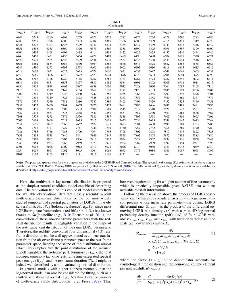
Now, with a statistical model for the observed rate of LGRBsat hand (i.e., Equation (5)), the best-fit parameters can beobtained by the method of maximum likelihood. This is doneby maximizing the likelihood function of the model, given the
Table 2Mean Best-fit Parameters of LGRB World Model, for
the Three Redshift Distribution Scenarios
Parameter HB06 Li (2008) B10
Redshift parameters (Equation (4))
z0 0.97 0.993 0.97z1 4.5 3.8 4.00γ0 3.4 3.3 3.14γ1 −0.3 0.0549 1.36γ2 −7.8 −4.46 −2.92
Location parameters
log(Liso) 51.35 ± 0.20 51.50 ± 0.19 51.73 ± 0.19log(Eiso) 51.82 ± 0.20 51.94 ± 0.20 52.03 ± 0.21log(Ep,z) 2.43 ± 0.05 2.47 ± 0.05 2.54 ± 0.05log(T90,z) 0.99 ± 0.03 0.96 ± 0.03 0.80 ± 0.03
Scale parameters
log(σLiso ) −0.22 ± 0.06 −0.23 ± 0.06 −0.20 ± 0.05log(σEiso ) −0.07 ± 0.03 −0.07 ± 0.03 −0.04 ± 0.03log(σEp,z ) −0.44 ± 0.02 −0.44 ± 0.02 −0.44 ± 0.02log(σT90,z
) −0.38 ± 0.01 −0.39 ± 0.01 −0.40 ± 0.01
Correlation coefficients
ρLiso−Eiso 0.93 ± 0.01 0.94 ± 0.01 0.96 ± 0.01ρLiso−Ep,z 0.47 ± 0.07 0.45 ± 0.07 0.44 ± 0.08ρLiso−T90,z
0.52 ± 0.08 0.59 ± 0.09 0.75 ± 0.07ρEiso−Ep,z 0.58 ± 0.04 0.58 ± 0.04 0.59 ± 0.04ρEiso−T90,z
0.63 ± 0.05 0.66 ± 0.05 0.74 ± 0.04ρEp,z−T90,z
0.34 ± 0.04 0.37 ± 0.04 0.50 ± 0.04
BATSE LGRB detection efficiency (Equation (A5))
μthresh −0.44 ± 0.02 −0.45 ± 0.02 −0.44 ± 0.02log(σthresh) −0.88 ± 0.05 −0.90 ± 0.05 −0.88 ± 0.05
Notes. The full Markov chain sampling of the above parameters from the16-dimensional parameter space of the likelihood function (Appendix C)is available for download at https://sites.google.com/site/amshportal/research/aca/in-the-news/lgrb-world-model for each of the three redshift distributions.
observational data, using a variant of the Metropolis–HastingsMarkov chain Monte Carlo (MCMC) algorithm discussed indetail in Appendix C. As mentioned before, the fitting isperformed for three redshift-distribution scenarios of HB06,B10, and Li (2008).
It is also known that the T90 of LGRBs are potentiallysubject to estimation biases. To ensure that the reported T90of BATSE LGRBs do not bias the fitting results for the rest ofthe parameters, model fitting was also performed by consideringonly three spectral variables of BATSE LGRBs: the bolometric1 s peak flux (Pbol), bolometric fluence (Sbol), and observed peakenergy (Ep), excluding duration (T90,z) variable from the model,thus reducing the dimension of the model by one. Only after thefitting was performed did it become clear that the inclusion ofthe T90 of BATSE LGRBs in the fitting does not significantlyaffect the resulting best-fit parameters of the model. Therefore,only results from the full model fitting are presented here, as inTable 2.
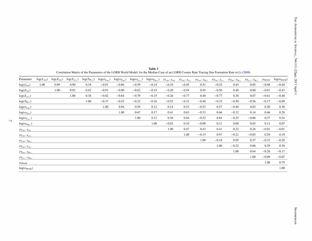
Due to lack of redshift information for BATSE GRBs, theresulting parameters of the model exhibit strong covariationswith each other. This is illustrated in the example correlationmatrix of the LGRB world model in Table 3. All location pa-rameters appear to correlate strongly positively with each other,and so do the scale parameters. The location parameters how-ever negatively correlate with the scale parameters, meaning
6
Th
eA
strophysical
Journ
al,766:111(22pp),2013
April1
Shah
moradi
Table 3Correlation Matrix of the Parameters of the LGRB World Model, for the Median Case of an LGRB Cosmic Rate Tracing Star Formation Rate in Li (2008)
Parameter log(Liso) log(Eiso) log(Ep,z) log(T90,z) log(σLiso ) log(σEiso ) log(σEp,z ) log(σT90,z) ρLiso−Eiso ρLiso−Ep,z ρLiso−T90,z
ρEiso−Ep,z ρEiso−T90,zρEp,z−T90,z
μthresh log(σthresh)
log(Liso) 1.00 0.99 0.90 0.34 −0.91 −0.86 −0.59 −0.14 −0.10 −0.45 0.51 −0.52 0.45 0.05 −0.68 −0.44
log(Eiso) 1.00 0.92 0.42 −0.91 −0.90 −0.62 −0.15 −0.20 −0.54 0.45 −0.56 0.40 0.00 −0.67 −0.43
log(Ep,z) 1.00 0.38 −0.82 −0.84 −0.79 −0.15 −0.26 −0.77 0.40 −0.77 0.38 0.07 −0.61 −0.40
log(T90,z) 1.00 −0.37 −0.52 −0.32 −0.16 −0.52 −0.32 −0.48 −0.33 −0.50 −0.56 −0.17 −0.09
log(σLiso ) 1.00 0.94 0.59 0.12 0.14 0.53 −0.53 0.57 −0.46 0.03 0.50 0.30
log(σEiso ) 1.00 0.67 0.17 0.41 0.63 −0.33 0.66 −0.32 0.14 0.46 0.28
log(σEp,z ) 1.00 0.12 0.36 0.84 −0.22 0.84 −0.25 −0.06 0.37 0.24
log(σT90,z) 1.00 −0.03 0.10 −0.09 0.11 0.00 0.03 0.11 0.07
ρLiso−Eiso 1.00 0.47 0.43 0.41 0.22 0.26 −0.01 −0.01
ρLiso−Ep,z 1.00 −0.15 0.97 −0.21 −0.05 0.29 0.19
ρLiso−T90,z1.00 −0.18 0.95 0.57 −0.32 −0.20
ρEiso−Ep,z 1.00 −0.22 0.06 0.29 0.18
ρEiso−T90,z1.00 0.64 −0.26 −0.17
ρEp,z−T90,z1.00 −0.09 −0.07
μthresh 1.00 0.79
log(σthresh) 1.00
7
The Astrophysical Journal, 766:111 (22pp), 2013 April 1 Shahmoradi
that an increase in the average values of the rest-frame parame-ters reduces the half-width of the corresponding distributions ofthe variables. In general, it is also observed that the correlationsamong the four variables weaken with increasing the locationparameters. An exception to this is the correlation of T90,z withLiso and Eiso which tends to increase with location parameters.Since an excess in the cosmic rates of LGRBs at high redshiftsgenerally results in an increase in the values of location param-eters, it can be said that “given BATSE LGRBs data, a higherrate for LGRBs at distant universe generally implies weakerEiso–Ep,z and Liso–Ep,z correlations and stronger covariationof T90,z with the three other parameters.”
2.4. Goodness-of-fit Tests
In any statistical fitting problem, perhaps more important thanthe model construction is to provide tests showing how goodthe model fit is to input data. For many univariate studies of theGRB LF, this is done by employing well-established statisticaltests such as the Kolmogorov–Smirnov (K-S; e.g., Kolmogoroff1941; Smirnov 1948) or Pearson’s χ2 (e.g., Fisher 1924) tests.In the case of multivariate studies (e.g., B10), a combination ofvisual inspection of the fitting results, K-S test on the marginal,and bivariate distributions and variants of χ2 (e.g., likelihoodratio) tests have been used.
In general, univariate tests on the marginal distributions ofmultivariate fits provide only necessary—but not sufficient—evidence for a good multivariate fit. Alternatively one couldassess the similarity by using nonparametric multivariate GoFtests. Such tests, although existing, have been rarely discussedand treated in statistics due to difficulties in the interpretationof the test statistic (e.g., Peacock 1983; Press et al. 1992; Justelet al. 1997). Ideally, one can always use the Pearson’s χ2 GoFtest for any multivariate distribution. However, for the specialcase of BATSE 1366 LGRBs, one would need an observedsample consisting of N � 1366 observations to avoid seriousinstabilities that occur in χ2 tests due to small sample sizes (e.g.,Cochran 1954).
To ensure a good fit to the observational data in all—and notonly univariate—levels of the multivariate structure of data, anassessment of similarity can be obtained by scanning and com-paring the model and data along their principal axes, in additionto univariate tests on the marginal distributions. Although statis-tically not a sufficient condition for the multivariate similarity ofthe model prediction to data, this can provide strong evidencein favor of a good fit, at a much higher confidence than testsperformed only on the marginal distributions.
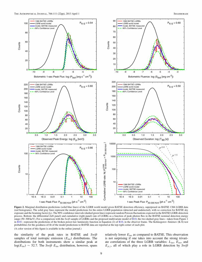
Following from above, Figure 2 presents the model predic-tions for marginal distributions of the four LGRB variables inthe observer frame. The K-S test probabilities for the similarityof the model predictions to the marginal distributions of BATSELGRB variables are also reported on the top right of each plot.All three redshift-distribution parameters of HB06, Li (2008),and B10 (Equation (4)) result in relatively similar fits to BATSEdata in the observer frame. Thus, for brevity, only plots for onerepresentative (median) redshift distribution (i.e., Li 2008) arepresented.
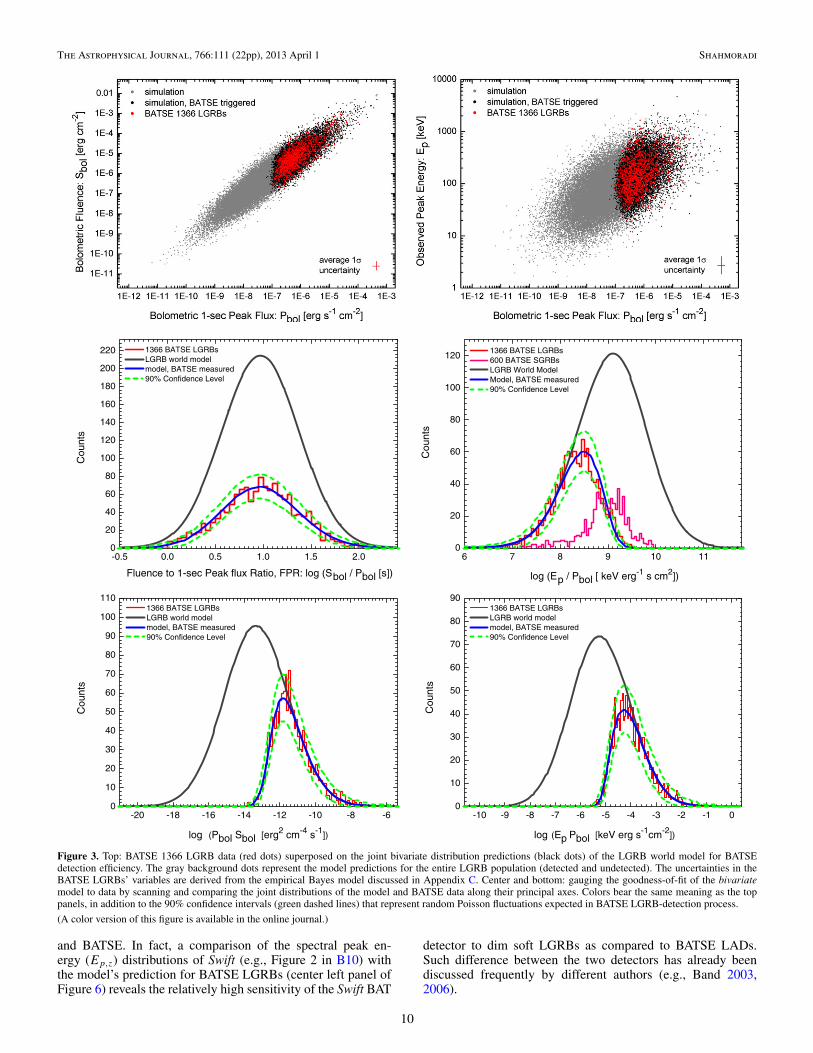
As the second level of GoF tests, the joint bivariate modelpredictions are compared to BATSE LGRB data, presented inFigures 3–5. This method of scanning model and data alongthe principal axes of the joint bivariate distributions can begeneralized to trivariate and quadruvariate joint distributions.For brevity, however, only the bivariate tests are presented.
3. RESULTS AND DISCUSSION
It is observed in the plots of Figures 2–5 that the modelprovides excellent fit to data, within the uncertainties causedby random Poisson fluctuations in the BATSE LGRB observedrate. These random fluctuations in BATSE detections are encom-passed in each graph by the green dashed lines that representthe 90% confidence intervals (CI) on BATSE LGRB detections(blue solid lines), derived by repeated sampling from the model.
Unfortunately, the same methods for a comparison of dataand model cannot be applied in the LGRB rest frame, due tolack of redshift information for the BATSE sample of LGRBs.Nevertheless, a comparison of the model with observational dataof other instruments—with measured redshifts—can provideclues on the underlying joint distribution of LGRB temporaland spectral variables in the rest frame compared to LGRBdetections of different gamma-ray instruments, as will be donein the following sections.
3.1. LGRB Luminosity Function and log(N )–log(P ) Diagram
The log(N )– log(P ) diagram of GRBs has been subject ofnumerous studies in the BATSE era, primarily for the purposeof finding signatures of cosmological (versus galactic) origins inthe LGRB rate. The cosmological origin of LGRBs is now wellestablished. Nevertheless, the log(N )– log(P ) diagram can stillprovide useful information for future gamma-ray experiments.
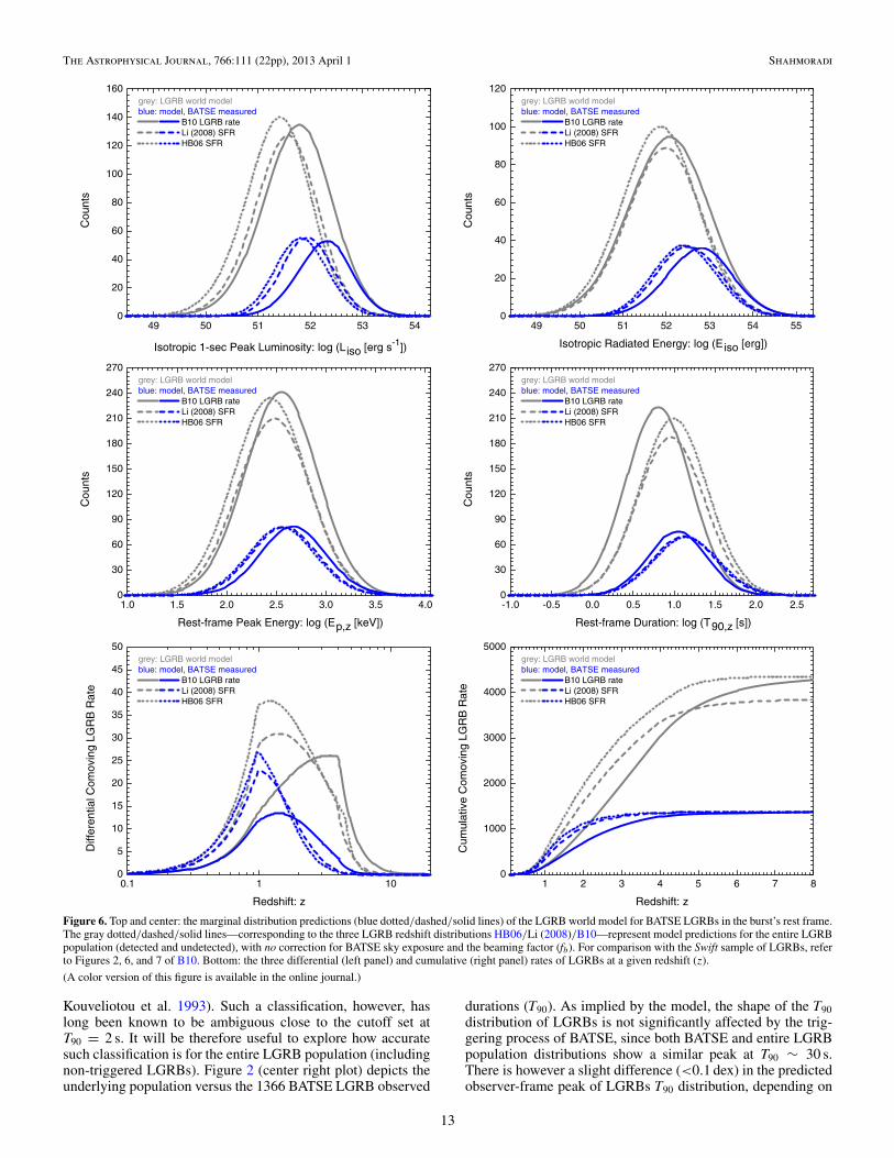
Figure 2 (bottom) depicts the prediction of the LGRB worldmodel for the traditional log(N )– log(P ) diagram for 1 speak photon flux in the BATSE nominal detection energyrange 50–300 keV, both for the differential (left panel) andthe cumulative (right panel) LGRB rate. For all three LGRBcosmic rates considered in this work—as in Table 2—thedifferential log(N )– log(P ) diagram shows a peak in the rate atP50–300 ∼ 0.1 photons s−1 cm−2. Such a peak in the LGRB rateresults in a relative flattening at the dim end of the cumulativelog(N )– log(P ) diagram, as compared to its bright end. Thisobservation has already been reported by B10 for the Swiftsample of LGRBs, although an entirely different LF—a brokenpower-law LF—was used by B10 in their multivariate LGRBworld model (cf. Equation (2) in B10).
On the other hand, the peak in the observer-frame LGRB ratetranslates to three relatively different (at ∼1σ level) peaks inthe LF of LGRBs. In general, it is observed that the peak of theLF (i.e., the average 1 s peak luminosity of LGRBs) increaseswith increasing cosmic rate of LGRBs at high redshift. Thiseffect is well depicted in the top left panel of Figure 6 forthe three LGRB cosmic rates considered: HB06, Li (2008),and B10.
Compared to the predictions of B10’s LGRB world model(cf. bottom plot of Figure 6 in B10), the log-normal modelsuggests a lower peak for BATSE LGRB LF (∼52.3 here versus∼52.7 in B10) for the same redshift distribution of LGRBs.Averaging over the three redshift distributions considered, themodel predicts a dynamic 3σ range of observer-frame brightnesslog(Pbol(erg s−1 cm−2)) ∈ [−7.11 ± 2.66] corresponding toPbol(erg s−1 cm−2) ∈ [1.70 × 10⁻¹⁰, 3.58 × 10⁻⁵] for LGRBs.This translates to an average dynamic 3σ range—in the restframe—of log(Liso(erg s−1)) ∈ [51.53±1.99] corresponding toLiso(erg s−1) ∈ [3.46 × 1049, 3.38 × 1053].
3.2. Isotropic Emission and Peak Energy Distributions
A comparison of the top-right panel of Figure 6 with Swiftobservations of LGRBs (e.g., B10, Figures 7 and 8) indicates
8
The Astrophysical Journal, 766:111 (22pp), 2013 April 1 Shahmoradi
-10 -9 -8 -7 -6 -5 -40
20
40
60
80
100
Cou
nts
Bolometric 1-sec Peak Flux: log (Pbol [erg s-1 cm-2])
1366 BATSE LGRBs LGRB world model model, BATSE measured 90% Confidence Level
PK-S = 0.54
-10 -9 -8 -7 -6 -5 -4 -30
10
20
30
40
50
60
70
80
90PK-S = 0.60
1366 BATSE LGRBs LGRB world model model, BATSE measured 90% Confidence Level
Cou
nts
Bolometric Fluence: log (Sbol [erg cm-2])
0.5 1.0 1.5 2.0 2.5 3.0 3.50
20
40
60
80
100
120
140
160
180
200
220PK-S = 0.60
Cou
nts
Observed Peak Energy: log (Ep [keV])
1366 BATSE LGRBs LGRB world model model, BATSE measured 90% Confidence Level
0.0 0.5 1.0 1.5 2.0 2.5 3.00
20
40
60
80
100
120
140
160
180
200
220
PK-S = 0.50 1366 BATSE LGRBs LGRB world model model, BATSE measured 90% Confidence Level
Cou
nts
Observed Duration: log (T90 [s])
1E-4 1E-3 0.01 0.1 1 10 1001
10
100
PK-S = 0.66 1366 BATSE LGRBs LGRB world model model, BATSE measured 90% Confidence Level
Cou
nts
1-sec Peak Flux: P50-300 KeV [ph s-1 cm-2]
1E-4 1E-3 0.01 0.1 1 10 1001
10
100
1000
10000
1366 BATSE LGRBs LGRB world model model, BATSE measured 90% Confidence Level
P-1.5
P-0.8
Cum
ulat
ive
LGR
B r
ate:
N(
PLG
RB
50-3
00 K
eV>
P50
-300
KeV
)
1-sec Peak Flux: P50-300 KeV [ph s-1 cm-2]
Figure 2. Marginal distribution predictions (solid blue lines) of the LGRB world model given BATSE detection efficiency, superposed on BATSE 1366 LGRB data(red histograms). The solid gray lines represent the model predictions for the entire LGRB population (detected and undetected), with no correction for BATSE skyexposure and the beaming factor (fb). The 90% confidence intervals (dashed green lines) represent random Poisson fluctuations expected in the BATSE LGRB-detectionprocess. Bottom: the differential (left panel) and cumulative (right panel) rate of LGRBs as a function of peak photon flux in the BATSE nominal detection energyrange (50–300 keV). For a comparison with the Swift sample of LGRBs and the proposed multivariate model of B10, the two dashed gray lines—taken from Figure 1in B10—represent the predictions of the broken power-law luminosity function in Equation (2) of B10, in the observer frame. The Kolmogorov–Smirnov (K-S) testprobabilities for the goodness-of-fit of the model predictions to BATSE data are reported at the top-right corner of each plot.
(A color version of this figure is available in the online journal.)
the similarity of the peak rates in BATSE and Swiftsamples of total isotropic emission (Eiso) distributions. Thedistributions for both instruments show a similar peak atlog(Eiso) ∼ 52.7. The Swift Eiso distribution, however, spans
relatively lower Eiso as compared to BATSE. This observationis not surprising if one takes into account the strong trivari-ate correlations of the three LGRB variables: Liso, Eiso, andEp,z, all of which play a role in LGRB detection by Swift
9
The Astrophysical Journal, 766:111 (22pp), 2013 April 1 Shahmoradi
-0.5 0.0 0.5 1.0 1.5 2.00
20
40
60
80
100
120
140
160
180
200
220
Cou
nts
Fluence to 1-sec Peak flux Ratio, FPR: log (Sbol / Pbol [s])
1366 BATSE LGRBs LGRB world model model, BATSE measured 90% Confidence Level
6 7 8 9 10 110
20
40
60
80
100
120
Cou
nts
log (Ep / Pbol [ keV erg-1 s cm2])
1366 BATSE LGRBs 600 BATSE SGRBs LGRB World Model Model, BATSE measured 90% Confidence Level
-20 -18 -16 -14 -12 -10 -8 -60
10
20
30
40
50
60
70
80
90
100
110 1366 BATSE LGRBs LGRB world model model, BATSE measured 90% Confidence Level
Cou
nts
log (Pbol Sbol [erg2 cm-4 s-1])
-10 -9 -8 -7 -6 -5 -4 -3 -2 -1 00
10
20
30
40
50
60
70
80
90 1366 BATSE LGRBs LGRB world model model, BATSE measured 90% Confidence Level
Cou
nts
log (Ep Pbol [keV erg s-1cm-2])
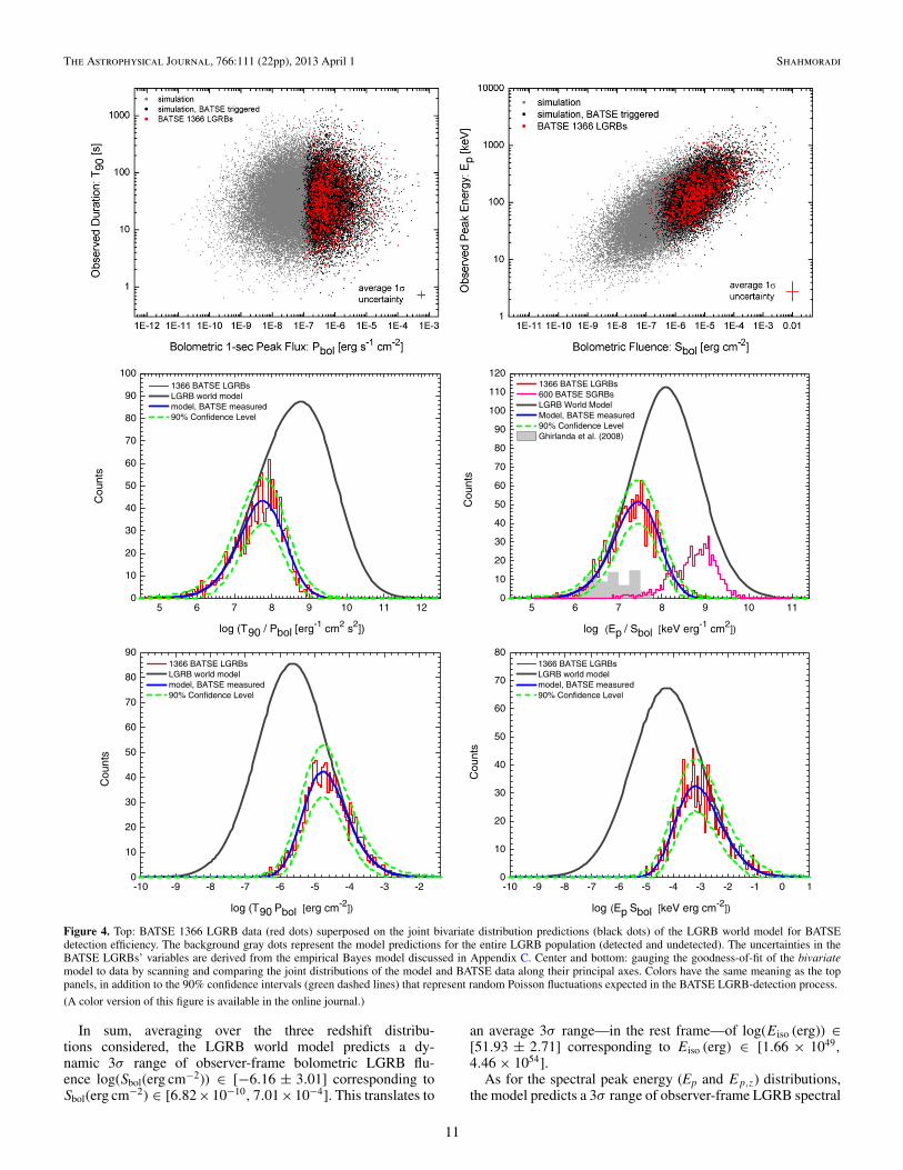
Figure 3. Top: BATSE 1366 LGRB data (red dots) superposed on the joint bivariate distribution predictions (black dots) of the LGRB world model for BATSEdetection efficiency. The gray background dots represent the model predictions for the entire LGRB population (detected and undetected). The uncertainties in theBATSE LGRBs’ variables are derived from the empirical Bayes model discussed in Appendix C. Center and bottom: gauging the goodness-of-fit of the bivariatemodel to data by scanning and comparing the joint distributions of the model and BATSE data along their principal axes. Colors bear the same meaning as the toppanels, in addition to the 90% confidence intervals (green dashed lines) that represent random Poisson fluctuations expected in BATSE LGRB-detection process.
(A color version of this figure is available in the online journal.)
and BATSE. In fact, a comparison of the spectral peak en-ergy (Ep,z) distributions of Swift (e.g., Figure 2 in B10) withthe model’s prediction for BATSE LGRBs (center left panel ofFigure 6) reveals the relatively high sensitivity of the Swift BAT
detector to dim soft LGRBs as compared to BATSE LADs.Such difference between the two detectors has already beendiscussed frequently by different authors (e.g., Band 2003,2006).
10
The Astrophysical Journal, 766:111 (22pp), 2013 April 1 Shahmoradi
5 6 7 8 9 10 11 120
10
20
30
40
50
60
70
80
90
100 1366 BATSE LGRBs LGRB world model model, BATSE measured 90% Confidence Level
Cou
nts
log (T90 / Pbol [erg-1 cm2 s2])
5 6 7 8 9 10 110
10
20
30
40
50
60
70
80
90
100
110
120 1366 BATSE LGRBs 600 BATSE SGRBs LGRB World Model Model, BATSE measured 90% Confidence Level Ghirlanda et al. (2008)
Cou
nts
log (Ep / Sbol [keV erg-1 cm2])
-10 -9 -8 -7 -6 -5 -4 -3 -20
10
20
30
40
50
60
70
80
90 1366 BATSE LGRBs LGRB world model model, BATSE measured 90% Confidence Level
Cou
nts
log (T90 Pbol [erg cm-2])
-10 -9 -8 -7 -6 -5 -4 -3 -2 -1 0 10
10
20
30
40
50
60
70
80 1366 BATSE LGRBs LGRB world model model, BATSE measured 90% Confidence Level
Cou
nts
log (Ep Sbol [keV erg cm-2])
Figure 4. Top: BATSE 1366 LGRB data (red dots) superposed on the joint bivariate distribution predictions (black dots) of the LGRB world model for BATSEdetection efficiency. The background gray dots represent the model predictions for the entire LGRB population (detected and undetected). The uncertainties in theBATSE LGRBs’ variables are derived from the empirical Bayes model discussed in Appendix C. Center and bottom: gauging the goodness-of-fit of the bivariatemodel to data by scanning and comparing the joint distributions of the model and BATSE data along their principal axes. Colors have the same meaning as the toppanels, in addition to the 90% confidence intervals (green dashed lines) that represent random Poisson fluctuations expected in the BATSE LGRB-detection process.
(A color version of this figure is available in the online journal.)
In sum, averaging over the three redshift distribu-tions considered, the LGRB world model predicts a dy-namic 3σ range of observer-frame bolometric LGRB flu-ence log(Sbol(erg cm−2)) ∈ [−6.16 ± 3.01] corresponding toSbol(erg cm−2) ∈ [6.82×10⁻¹⁰, 7.01×10⁻⁴]. This translates to
an average 3σ range—in the rest frame—of log(Eiso (erg)) ∈[51.93 ± 2.71] corresponding to Eiso (erg) ∈ [1.66 × 1049,4.46 × 1054].
As for the spectral peak energy (Ep and Ep,z) distributions,the model predicts a 3σ range of observer-frame LGRB spectral
11
The Astrophysical Journal, 766:111 (22pp), 2013 April 1 Shahmoradi
4 5 6 7 8 9 10 110
10
20
30
40
50
60
70
80
90
100 1366 BATSE LGRBs LGRB World Model Model, BATSE measured 90% Confidence Level
Cou
nts
log (T90 / Sbol [erg-1 cm2 s])
-1.5 -1.0 -0.5 0.0 0.5 1.0 1.5 2.0 2.50
20
40
60
80
100
120
140
160
180 1366 BATSE LGRBs LGRB world model model, BATSE measured 90% Confidence Level
Cou
nts
log (Ep / T90 [keV s-1])
-10 -9 -8 -7 -6 -5 -4 -3 -2 -1 00
10
20
30
40
50
60
70
80 1366 BATSE LGRBs LGRB world model model, BATSE measured 90% Confidence Level
Cou
nts
log (T90 Sbol [s erg cm-2])
1 2 3 4 5 60
20
40
60
80
100
120
140
160 1366 BATSE LGRBs LGRB world model model, BATSE measured 90% Confidence Level
Cou
nts
log (Ep T90 [keV s])
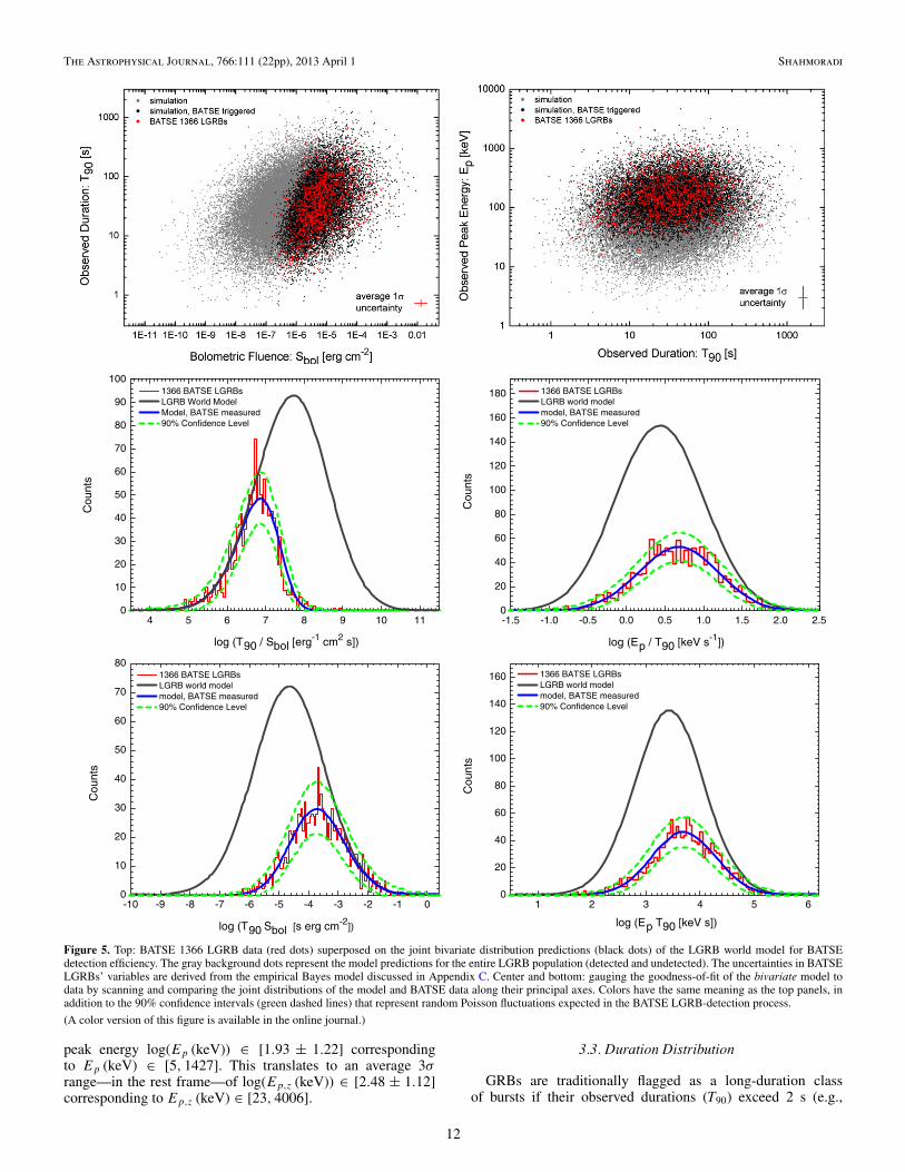
Figure 5. Top: BATSE 1366 LGRB data (red dots) superposed on the joint bivariate distribution predictions (black dots) of the LGRB world model for BATSEdetection efficiency. The gray background dots represent the model predictions for the entire LGRB population (detected and undetected). The uncertainties in BATSELGRBs’ variables are derived from the empirical Bayes model discussed in Appendix C. Center and bottom: gauging the goodness-of-fit of the bivariate model todata by scanning and comparing the joint distributions of the model and BATSE data along their principal axes. Colors have the same meaning as the top panels, inaddition to the 90% confidence intervals (green dashed lines) that represent random Poisson fluctuations expected in the BATSE LGRB-detection process.
(A color version of this figure is available in the online journal.)
peak energy log(Ep (keV)) ∈ [1.93 ± 1.22] correspondingto Ep (keV) ∈ [5, 1427]. This translates to an average 3σrange—in the rest frame—of log(Ep,z (keV)) ∈ [2.48 ± 1.12]corresponding to Ep,z (keV) ∈ [23, 4006].
3.3. Duration Distribution
GRBs are traditionally flagged as a long-duration classof bursts if their observed durations (T90) exceed 2 s (e.g.,
12
The Astrophysical Journal, 766:111 (22pp), 2013 April 1 Shahmoradi
49 50 51 52 53 540
20
40
60
80
100
120
140
160C
ount
s
Isotropic 1-sec Peak Luminosity: log (Liso [erg s-1])
grey: LGRB world modelblue: model, BATSE measured
B10 LGRB rate Li (2008) SFR HB06 SFR
49 50 51 52 53 54 550
20
40
60
80
100
120grey: LGRB world modelblue: model, BATSE measured
B10 LGRB rate Li (2008) SFR HB06 SFR
Cou
nts
Isotropic Radiated Energy: log (Eiso [erg])
1.0 1.5 2.0 2.5 3.0 3.5 4.00
30
60
90
120
150
180
210
240
270grey: LGRB world modelblue: model, BATSE measured
B10 LGRB rate Li (2008) SFR HB06 SFR
Cou
nts
Rest-frame Peak Energy: log (Ep,z [keV])
-1.0 -0.5 0.0 0.5 1.0 1.5 2.0 2.50
30
60
90
120
150
180
210
240
270grey: LGRB world modelblue: model, BATSE measured
B10 LGRB rate Li (2008) SFR HB06 SFR
Cou
nts
Rest-frame Duration: log (T90,z [s])
0111.00
5
10
15
20
25
30
35
40
45
50grey: LGRB world modelblue: model, BATSE measured
B10 LGRB rate Li (2008) SFR HB06 SFR
Diff
eren
tial C
omov
ing
LGR
B R
ate
Redshift: z
1 2 3 4 5 6 7 80
1000
2000
3000
4000
5000grey: LGRB world modelblue: model, BATSE measured
B10 LGRB rate Li (2008) SFR HB06 SFR
Cum
ulat
ive
Com
ovin
g LG
RB
Rat
e
Redshift: z
Figure 6. Top and center: the marginal distribution predictions (blue dotted/dashed/solid lines) of the LGRB world model for BATSE LGRBs in the burst’s rest frame.The gray dotted/dashed/solid lines—corresponding to the three LGRB redshift distributions HB06/Li (2008)/B10—represent model predictions for the entire LGRBpopulation (detected and undetected), with no correction for BATSE sky exposure and the beaming factor (fb). For comparison with the Swift sample of LGRBs, referto Figures 2, 6, and 7 of B10. Bottom: the three differential (left panel) and cumulative (right panel) rates of LGRBs at a given redshift (z).
(A color version of this figure is available in the online journal.)
Kouveliotou et al. 1993). Such a classification, however, haslong been known to be ambiguous close to the cutoff set atT90 = 2 s. It will be therefore useful to explore how accuratesuch classification is for the entire LGRB population (includingnon-triggered LGRBs). Figure 2 (center right plot) depicts theunderlying population versus the 1366 BATSE LGRB observed
durations (T90). As implied by the model, the shape of the T90distribution of LGRBs is not significantly affected by the trig-gering process of BATSE, since both BATSE and entire LGRBpopulation distributions show a similar peak at T90 ∼ 30 s.There is however a slight difference (<0.1 dex) in the predictedobserver-frame peak of LGRBs T90 distribution, depending on
13
The Astrophysical Journal, 766:111 (22pp), 2013 April 1 Shahmoradi
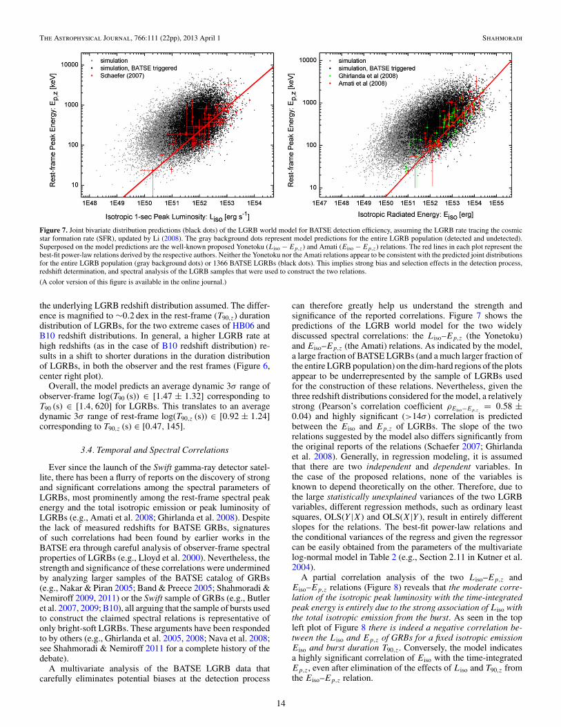
Figure 7. Joint bivariate distribution predictions (black dots) of the LGRB world model for BATSE detection efficiency, assuming the LGRB rate tracing the cosmicstar formation rate (SFR), updated by Li (2008). The gray background dots represent model predictions for the entire LGRB population (detected and undetected).Superposed on the model predictions are the well-known proposed Yonetoku (Liso − Ep,z) and Amati (Eiso − Ep,z) relations. The red lines in each plot represent thebest-fit power-law relations derived by the respective authors. Neither the Yonetoku nor the Amati relations appear to be consistent with the predicted joint distributionsfor the entire LGRB population (gray background dots) or 1366 BATSE LGRBs (black dots). This implies strong bias and selection effects in the detection process,redshift determination, and spectral analysis of the LGRB samples that were used to construct the two relations.
(A color version of this figure is available in the online journal.)
the underlying LGRB redshift distribution assumed. The differ-ence is magnified to ∼0.2 dex in the rest-frame (T90,z) durationdistribution of LGRBs, for the two extreme cases of HB06 andB10 redshift distributions. In general, a higher LGRB rate athigh redshifts (as in the case of B10 redshift distribution) re-sults in a shift to shorter durations in the duration distributionof LGRBs, in both the observer and the rest frames (Figure 6,center right plot).
Overall, the model predicts an average dynamic 3σ range ofobserver-frame log(T90 (s)) ∈ [1.47 ± 1.32] corresponding toT90 (s) ∈ [1.4, 620] for LGRBs. This translates to an averagedynamic 3σ range of rest-frame log(T90,z (s)) ∈ [0.92 ± 1.24]corresponding to T90,z (s) ∈ [0.47, 145].
3.4. Temporal and Spectral Correlations
Ever since the launch of the Swift gamma-ray detector satel-lite, there has been a flurry of reports on the discovery of strongand significant correlations among the spectral parameters ofLGRBs, most prominently among the rest-frame spectral peakenergy and the total isotropic emission or peak luminosity ofLGRBs (e.g., Amati et al. 2008; Ghirlanda et al. 2008). Despitethe lack of measured redshifts for BATSE GRBs, signaturesof such correlations had been found by earlier works in theBATSE era through careful analysis of observer-frame spectralproperties of LGRBs (e.g., Lloyd et al. 2000). Nevertheless, thestrength and significance of these correlations were underminedby analyzing larger samples of the BATSE catalog of GRBs(e.g., Nakar & Piran 2005; Band & Preece 2005; Shahmoradi &Nemiroff 2009, 2011) or the Swift sample of GRBs (e.g., Butleret al. 2007, 2009; B10), all arguing that the sample of bursts usedto construct the claimed spectral relations is representative ofonly bright-soft LGRBs. These arguments have been respondedto by others (e.g., Ghirlanda et al. 2005, 2008; Nava et al. 2008;see Shahmoradi & Nemiroff 2011 for a complete history of thedebate).
A multivariate analysis of the BATSE LGRB data thatcarefully eliminates potential biases at the detection process
can therefore greatly help us understand the strength andsignificance of the reported correlations. Figure 7 shows thepredictions of the LGRB world model for the two widelydiscussed spectral correlations: the Liso–Ep,z (the Yonetoku)and Eiso–Ep,z (the Amati) relations. As indicated by the model,a large fraction of BATSE LGRBs (and a much larger fraction ofthe entire LGRB population) on the dim-hard regions of the plotsappear to be underrepresented by the sample of LGRBs usedfor the construction of these relations. Nevertheless, given thethree redshift distributions considered for the model, a relativelystrong (Pearson’s correlation coefficient ρEiso−Ep,z
= 0.58 ±0.04) and highly significant (>14σ ) correlation is predictedbetween the Eiso and Ep,z of LGRBs. The slope of the tworelations suggested by the model also differs significantly fromthe original reports of the relations (Schaefer 2007; Ghirlandaet al. 2008). Generally, in regression modeling, it is assumedthat there are two independent and dependent variables. Inthe case of the proposed relations, none of the variables isknown to depend theoretically on the other. Therefore, due tothe large statistically unexplained variances of the two LGRBvariables, different regression methods, such as ordinary leastsquares, OLS(Y |X) and OLS(X|Y ), result in entirely differentslopes for the relations. The best-fit power-law relations andthe conditional variances of the regress and given the regressorcan be easily obtained from the parameters of the multivariatelog-normal model in Table 2 (e.g., Section 2.11 in Kutner et al.2004).
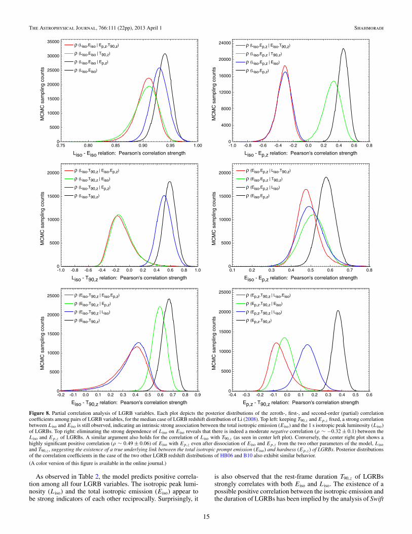
A partial correlation analysis of the two Liso–Ep,z andEiso–Ep,z relations (Figure 8) reveals that the moderate corre-lation of the isotropic peak luminosity with the time-integratedpeak energy is entirely due to the strong association of Liso withthe total isotropic emission from the burst. As seen in the topleft plot of Figure 8 there is indeed a negative correlation be-tween the Liso and Ep,z of GRBs for a fixed isotropic emissionEiso and burst duration T90,z. Conversely, the model indicatesa highly significant correlation of Eiso with the time-integratedEp,z, even after elimination of the effects of Liso and T90,z fromthe Eiso–Ep,z relation.
14
The Astrophysical Journal, 766:111 (22pp), 2013 April 1 Shahmoradi
0.75 0.80 0.85 0.90 0.95 1.000
5000
10000
15000
20000
25000
30000
35000 ρ (Liso,Eiso | Ep,z,T90,z)
ρ (Liso,Eiso | T90,z)
ρ (Liso,Eiso | Ep,z)
ρ (Liso,Eiso)
MC
MC
sam
plin
g co
unts
Liso - Eiso relation: Pearson's correlation strength
-1.0 -0.8 -0.6 -0.4 -0.2 0.0 0.2 0.4 0.6 0.80
4000
8000
12000
16000
20000
24000
MC
MC
sam
plin
g co
unts
Liso - Ep,z relation: Pearson's correlation strength
ρ (Liso,Ep,z | Eiso,T90,z)
ρ (Liso,Ep,z | T90,z)
ρ (Liso,Ep,z | Eiso)
ρ (Liso,Ep,z)
-1.0 -0.8 -0.6 -0.4 -0.2 0.0 0.2 0.4 0.6 0.8 1.00
5000
10000
15000
20000ρ (Liso,T90,z | Eiso,Ep,z)
ρ (Liso,T90,z | Eiso)
ρ (Liso,T90,z | Ep,z)
ρ (Liso,T90,z)
MC
MC
sam
plin
g co
unts
Liso - T90,z relation: Pearson's correlation strength
0.1 0.2 0.3 0.4 0.5 0.6 0.7 0.80
5000
10000
15000
20000ρ (Eiso,Ep,z | Liso,T90,z)
ρ (Eiso,Ep,z | T90,z)
ρ (Eiso,Ep,z | Liso)
ρ (Eiso,Ep,z)
MC
MC
sam
plin
g co
unts
Eiso - Ep,z relation: Pearson's correlation strength
-0.2 -0.1 0.0 0.1 0.2 0.3 0.4 0.5 0.6 0.7 0.8 0.90
5000
10000
15000
20000
25000 ρ (Eiso,T90,z | Eiso,Ep,z)
ρ (Eiso,T90,z | Ep,z)
ρ (Eiso,T90,z | Liso)
ρ (Eiso,T90,z)
MC
MC
sam
plin
g co
unts
Eiso - T90,z relation: Pearson's correlation strength
-0.4 -0.3 -0.2 -0.1 0.0 0.1 0.2 0.3 0.4 0.5 0.60
5000
10000
15000
20000
25000 ρ (Ep,z,T90,z | Liso,Eiso)
ρ (Ep,z,T90,z | Eiso)
ρ (Ep,z,T90,z | Liso)
ρ (Ep,z,T90,z)
MC
MC
sam
plin
g co
unts
Ep,z - T90,z relation: Pearson's correlation strength
Figure 8. Partial correlation analysis of LGRB variables. Each plot depicts the posterior distributions of the zeroth-, first-, and second-order (partial) correlationcoefficients among pairs of LGRB variables, for the median case of LGRB redshift distribution of Li (2008). Top left: keeping T90,z and Ep,z fixed, a strong correlationbetween Liso and Eiso is still observed, indicating an intrinsic strong association between the total isotropic emission (Eiso) and the 1 s isotropic peak luminosity (Liso)of LGRBs. Top right: eliminating the strong dependence of Liso on Eiso reveals that there is indeed a moderate negative correlation (ρ ∼ −0.32 ± 0.1) between theLiso and Ep,z of LGRBs. A similar argument also holds for the correlation of Liso with T90,z (as seen in center left plot). Conversely, the center right plot shows ahighly significant positive correlation (ρ ∼ 0.49 ± 0.06) of Eiso with Ep,z even after dissociation of Eiso and Ep,z from the two other parameters of the model, Lisoand T90,z, suggesting the existence of a true underlying link between the total isotropic prompt emission (Eiso) and hardness (Ep,z) of LGRBs. Posterior distributionsof the correlation coefficients in the case of the two other LGRB redshift distributions of HB06 and B10 also exhibit similar behavior.
(A color version of this figure is available in the online journal.)
As observed in Table 2, the model predicts positive correla-tion among all four LGRB variables. The isotropic peak lumi-nosity (Liso) and the total isotropic emission (Eiso) appear tobe strong indicators of each other reciprocally. Surprisingly, it
is also observed that the rest-frame duration T90,z of LGRBsstrongly correlates with both Eiso and Liso. The existence of apossible positive correlation between the isotropic emission andthe duration of LGRBs has been implied by the analysis of Swift
15
The Astrophysical Journal, 766:111 (22pp), 2013 April 1 Shahmoradi
0.01 0.1 1 10 100 10001E-3
0.01
0.1
1
10
100
1000 90% Confidence Intervals
diffe
rent
ial 1
966
BA
TS
E T
90 c
ount
s: d
N /
dT90
Observed Duration: T90 [s]
BATSE 1966 T90 distribution
BATSE 1366 T90 distribution
BATSE 600 T90 distribution
LGRB world model prediction
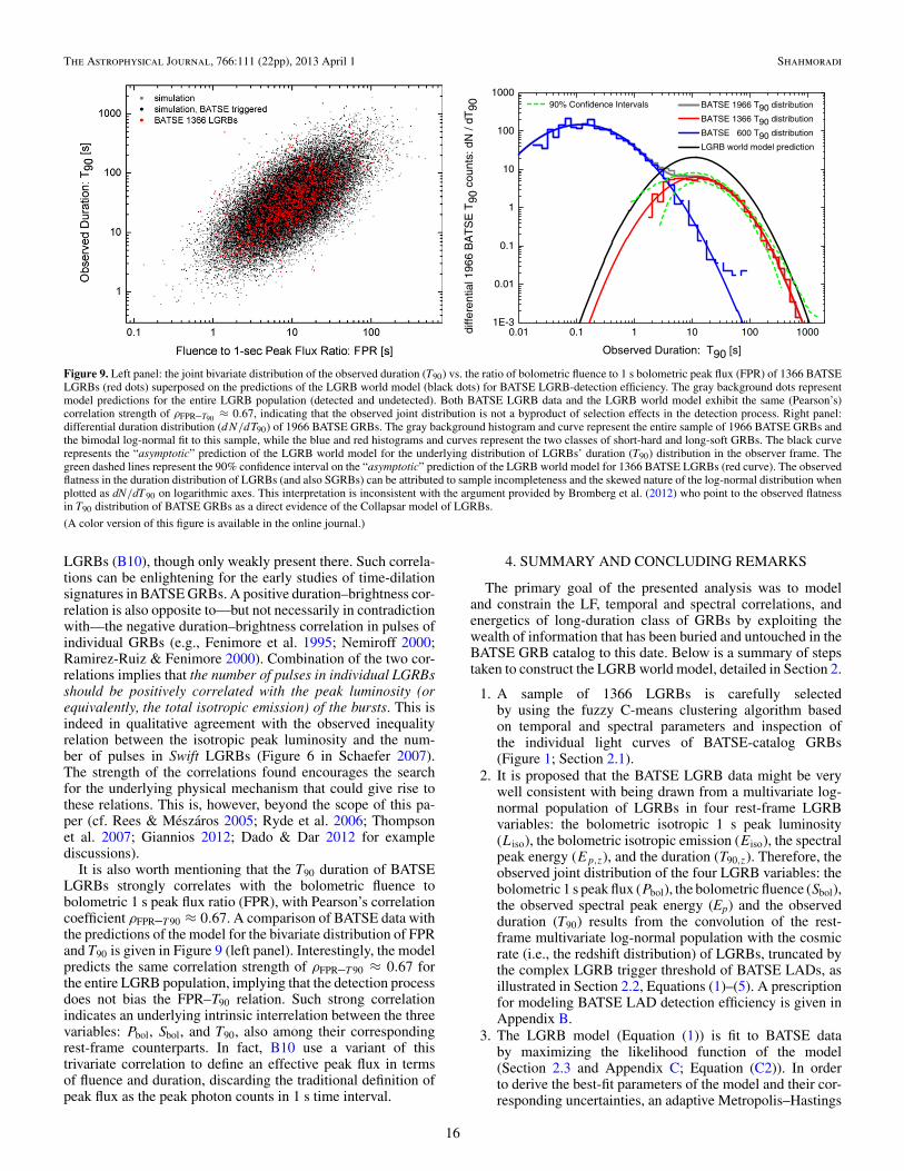
Figure 9. Left panel: the joint bivariate distribution of the observed duration (T90) vs. the ratio of bolometric fluence to 1 s bolometric peak flux (FPR) of 1366 BATSELGRBs (red dots) superposed on the predictions of the LGRB world model (black dots) for BATSE LGRB-detection efficiency. The gray background dots representmodel predictions for the entire LGRB population (detected and undetected). Both BATSE LGRB data and the LGRB world model exhibit the same (Pearson’s)correlation strength of ρFPR–T90 ≈ 0.67, indicating that the observed joint distribution is not a byproduct of selection effects in the detection process. Right panel:differential duration distribution (dN/dT90) of 1966 BATSE GRBs. The gray background histogram and curve represent the entire sample of 1966 BATSE GRBs andthe bimodal log-normal fit to this sample, while the blue and red histograms and curves represent the two classes of short-hard and long-soft GRBs. The black curverepresents the “asymptotic” prediction of the LGRB world model for the underlying distribution of LGRBs’ duration (T90) distribution in the observer frame. Thegreen dashed lines represent the 90% confidence interval on the “asymptotic” prediction of the LGRB world model for 1366 BATSE LGRBs (red curve). The observedflatness in the duration distribution of LGRBs (and also SGRBs) can be attributed to sample incompleteness and the skewed nature of the log-normal distribution whenplotted as dN/dT90 on logarithmic axes. This interpretation is inconsistent with the argument provided by Bromberg et al. (2012) who point to the observed flatnessin T90 distribution of BATSE GRBs as a direct evidence of the Collapsar model of LGRBs.
(A color version of this figure is available in the online journal.)
LGRBs (B10), though only weakly present there. Such correla-tions can be enlightening for the early studies of time-dilationsignatures in BATSE GRBs. A positive duration–brightness cor-relation is also opposite to—but not necessarily in contradictionwith—the negative duration–brightness correlation in pulses ofindividual GRBs (e.g., Fenimore et al. 1995; Nemiroff 2000;Ramirez-Ruiz & Fenimore 2000). Combination of the two cor-relations implies that the number of pulses in individual LGRBsshould be positively correlated with the peak luminosity (orequivalently, the total isotropic emission) of the bursts. This isindeed in qualitative agreement with the observed inequalityrelation between the isotropic peak luminosity and the num-ber of pulses in Swift LGRBs (Figure 6 in Schaefer 2007).The strength of the correlations found encourages the searchfor the underlying physical mechanism that could give rise tothese relations. This is, however, beyond the scope of this pa-per (cf. Rees & Meszaros 2005; Ryde et al. 2006; Thompsonet al. 2007; Giannios 2012; Dado & Dar 2012 for examplediscussions).
It is also worth mentioning that the T90 duration of BATSELGRBs strongly correlates with the bolometric fluence tobolometric 1 s peak flux ratio (FPR), with Pearson’s correlationcoefficient ρFPR–T 90 ≈ 0.67. A comparison of BATSE data withthe predictions of the model for the bivariate distribution of FPRand T90 is given in Figure 9 (left panel). Interestingly, the modelpredicts the same correlation strength of ρFPR–T 90 ≈ 0.67 forthe entire LGRB population, implying that the detection processdoes not bias the FPR–T90 relation. Such strong correlationindicates an underlying intrinsic interrelation between the threevariables: Pbol, Sbol, and T90, also among their correspondingrest-frame counterparts. In fact, B10 use a variant of thistrivariate correlation to define an effective peak flux in termsof fluence and duration, discarding the traditional definition ofpeak flux as the peak photon counts in 1 s time interval.
4. SUMMARY AND CONCLUDING REMARKS
The primary goal of the presented analysis was to modeland constrain the LF, temporal and spectral correlations, andenergetics of long-duration class of GRBs by exploiting thewealth of information that has been buried and untouched in theBATSE GRB catalog to this date. Below is a summary of stepstaken to construct the LGRB world model, detailed in Section 2.
1. A sample of 1366 LGRBs is carefully selectedby using the fuzzy C-means clustering algorithm basedon temporal and spectral parameters and inspection ofthe individual light curves of BATSE-catalog GRBs(Figure 1; Section 2.1).
2. It is proposed that the BATSE LGRB data might be verywell consistent with being drawn from a multivariate log-normal population of LGRBs in four rest-frame LGRBvariables: the bolometric isotropic 1 s peak luminosity(Liso), the bolometric isotropic emission (Eiso), the spectralpeak energy (Ep,z), and the duration (T90,z). Therefore, theobserved joint distribution of the four LGRB variables: thebolometric 1 s peak flux (Pbol), the bolometric fluence (Sbol),the observed spectral peak energy (Ep) and the observedduration (T90) results from the convolution of the rest-frame multivariate log-normal population with the cosmicrate (i.e., the redshift distribution) of LGRBs, truncated bythe complex LGRB trigger threshold of BATSE LADs, asillustrated in Section 2.2, Equations (1)–(5). A prescriptionfor modeling BATSE LAD detection efficiency is given inAppendix B.
3. The LGRB model (Equation (1)) is fit to BATSE databy maximizing the likelihood function of the model(Section 2.3 and Appendix C; Equation (C2)). In orderto derive the best-fit parameters of the model and their cor-responding uncertainties, an adaptive Metropolis–Hastings
16
The Astrophysical Journal, 766:111 (22pp), 2013 April 1 Shahmoradi
MCMC (AMH-MCMC) algorithm is set up to efficientlysample from the 16D likelihood function. The best-fit pa-rameters are obtained for three LGRB cosmic rates: SFR ofHB06, SFR of Li (2008), and the predicted LGRB redshiftdistribution of B10 which is consistent with the LGRB ratetracing cosmic metallicity with a cutoff Z/Z� ∼ 0.2–0.5.
4. To ensure the model provides adequate fit to observationaldata, multivariate GoF tests are presented (Section 2.4 andFigures 2–5).
Summarized below are the principal conclusions drawn fromthe analysis based on the proposed LGRB world model.
1. Energetics. It is expected that the peak brightnessdistribution of LGRBs has the effective range oflog(Pbol(erg s−1 cm−2)) ∈ [−7.11 ± 2.66] correspondingto Pbol(erg s−1 cm−2) ∈ [1.70 × 10⁻¹⁰, 3.58 × 10⁻⁵]. Thistranslates to a dynamic 3σ range—in the rest frame—oflog(Liso(erg s−1)) ∈ [51.53 ± 1.99], corresponding toLiso(erg s−1) ∈ [3.46 × 1049, 3.38 × 1053]. In addition,a turnover is predicted in the differential log(N )– log(P )diagram of LGRBs at P50–300 ∼ 0.1 photons s−1 cm−2 inthe BATSE nominal detection energy range (50–300 keV).This is consistent with and further extends the apparent flat-tening in the cumulative log(N )– log(P ) diagram of SwiftLGRBs reported recently by B10.
As for the bolometric fluence and the total isotropicemission distributions, a range of log(Sbol(erg cm−2)) ∈[−6.16 ± 3.01] corresponding to Sbol(erg cm−2) ∈[6.82 × 10⁻¹⁰, 7.01 × 10⁻⁴] is indicated. This trans-lates to an average dynamic 3σ range—in the restframe—of log(Eiso (erg)) ∈ [51.93 ± 2.71] correspondingto Eiso (erg) ∈ [1.66 × 1049, 4.46 × 1054] (Sections 3.2and 3.1; Table 2).
2. Durations and spectral peak energies. The rest-framespectral peak energies (Ep,z) of LGRBs are likely welldescribed by a log-normal distribution with an average 3σrange of log(Ep,z (keV)) ∈ [2.48 ± 1.12] correspondingto Ep,z (keV) ∈ [23, 4006] with peak LGRB rate atEp,z ∼ 300 (keV). This translates to an effective observer-frame peak energy range of log(Ep (keV)) ∈ [1.93 ± 1.22]corresponding to Ep (keV) ∈ [5, 1427] with peak LGRBrate at Ep ∼ 85 keV. It is also observed that the observer-frame T90 duration of LGRBs peaks at T90 ∼ 30 s witha 3σ range of T90 (s) ∈ [1.4, 620]. This translates to anaverage 3σ range of rest-frame log(T90,z (s)) ∈ [0.92±1.24]corresponding to T90,z (s) ∈ [0.47, 145] with a peak rate atT90,z ∼ 10 s (Section 3.3; Table 2).
Recently, Bromberg et al. (2012) proposed the apparentflatness in the duration distribution of BATSE LGRBs—when plotted in the form of dN/dT90 instead ofdN/d log(T90)—as the first direct evidence of the Collap-sar model of LGRBs. The results of presented analysis areinconsistent with a flat T90 distribution of LGRBs at shortdurations (Figure 2, center right panel and Figure 9, rightpanel). The observed flat T90 distribution of LGRBs at shortdurations can be explained away in terms of the skewednature of the log-normal distribution subject to sample in-completeness. It is therefore expected that a significantlylarger sample of LGRBs that will be detected by futuregamma-ray satellites will smear out the apparent flatnessat the short tail of the duration distribution of LGRBs. Asimilar flat distribution is also observed for SGRBs at veryshort durations (Figure 9, right panel) which might be hard
to reconcile with the Collapsar interpretation of the ob-served flatness in the LGRB T90 distribution, proposed byBromberg et al. (2012).
3. Temporal and spectral correlations. All four LGRB vari-ables: Liso, Eiso, Ep,z, and T90,z appear to be either mod-erately or strongly positively correlated with each other. Inparticular, a relatively strong and “broad” but highly signif-icant correlation strength (Pearson’s correlation coefficientρEiso−Ep,z
= 0.58±0.04) is predicted between Eiso and Ep,z
of long-duration class of GRBs. Surprisingly, T90,z appearsto evolve with Liso and Eiso such that brighter bursts gen-erally tend to have longer durations (Section 3.4; Table 2).This prediction of the model together with the previouslyreported negative correlation of the brightness and the du-ration of individual pulses in LGRBs (e.g., Fenimore et al.1995; Nemiroff 2000; Ramirez-Ruiz & Fenimore 2000)might possibly indicate that intrinsically brighter LGRBscontain, on average, a higher number of pulses.
There is a slight chance that a small fraction (<50)of BATSE LGRBs were misclassified as SGRBs by theautomated pattern recognition methods exploited in thisanalysis (see Figure 3, center right panel). If true, it willmost likely affect (if significant at all) the constraintsderived on the LF of LGRBs and the correlation of Ep,z
with Liso.4. Redshift distribution. The lack redshift information for the
BATSE GRBs strongly limits the prediction power of thepresented analysis for the cosmic rate of LGRBs. Neverthe-less, based on the Markov chain sampling of the likelihoodfunction for the three LGRB redshift distributions consid-ered here (Section 2.2 and Figure 10), it is observed thatBATSE data potentially, but not necessarily, favor an LGRBrate consistent with cosmic metallicity evolution with a cut-off Z/Z� ∼ 0.2–0.5 (cf. B10), with no luminosity–redshiftevolution.
Assuming that LGRBs track SFR, only a tiny fraction(i.e., ∼2–3) of 1366 BATSE LGRBs are expected to haveoriginated from high redshifts (z � 5). In the case ofan LGRB rate tracing cosmic metallicity evolution (e.g.,B10), the fraction increases by one order of magnitude to∼2%, corresponding to ∼27 bursts out of 1366 BATSELGRBs. For comparison, the expected fraction of Swiftand EXIST LGRBs with z � 5 are ∼6% and ∼7%(B10). The discrepancy is well explained by the factthat both Swift and EXIST are more sensitive to long-soft bursts—characteristic of high-redshift LGRBs—due totheir lower gamma-ray trigger energy window, comparedto BATSE DADs (cf. Gehrels et al. 2004; Band et al. 2008;Grindlay & the EXIST Team 2009).
Although fitting is performed for the rest-frame variables,it is notable that the overall shape of the resulting observer-frame distribution of the variables also resembles a multivari-ate log-normal (see Figures 2–7). In other words, the redshiftconvolution of the rest-frame population distribution approx-imately acts as a linear transformation from the rest frame ofLGRBs to the observer frame. This is primarily due to the narrowredshift distribution of LGRBs—as compared to the width ofthe LGRB rest-frame temporal and spectral distributions—withalmost 90% of the population originating from intermediateredshifts, z ∈ [1, 4.3]. Balazs et al. (2003) provide an ele-gant discussion on the potential effects of redshift convolutionon the observed distribution of LGRB durations and spectralparameters.
17
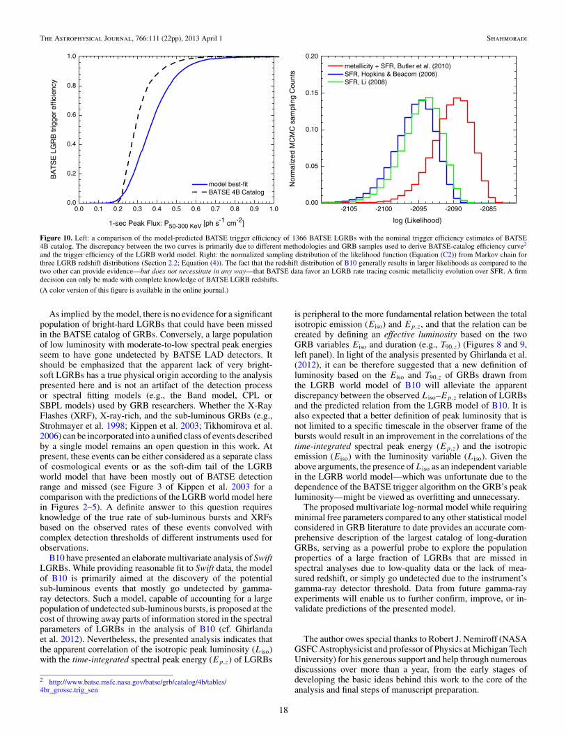
The Astrophysical Journal, 766:111 (22pp), 2013 April 1 Shahmoradi
0.0 0.1 0.2 0.3 0.4 0.5 0.6 0.7 0.8 0.9 1.00.0
0.2
0.4
0.6
0.8
1.0B
AT
SE
LG
RB
trig
ger
effic
ienc
y
1-sec Peak Flux: P50-300 KeV [ph s-1 cm-2]
model best-fit BATSE 4B Catalog
-2105 -2100 -2095 -2090 -20850.00
0.05
0.10
0.15
0.20
Nor
mal
ized
MC
MC
sam
plin
g C
ount
s
log (Likelihood)
metallicity + SFR, Butler et al. (2010) SFR, Hopkins & Beacom (2006) SFR, Li (2008)
Figure 10. Left: a comparison of the model-predicted BATSE trigger efficiency of 1366 BATSE LGRBs with the nominal trigger efficiency estimates of BATSE4B catalog. The discrepancy between the two curves is primarily due to different methodologies and GRB samples used to derive BATSE-catalog efficiency curve2
and the trigger efficiency of the LGRB world model. Right: the normalized sampling distribution of the likelihood function (Equation (C2)) from Markov chain forthree LGRB redshift distributions (Section 2.2; Equation (4)). The fact that the redshift distribution of B10 generally results in larger likelihoods as compared to thetwo other can provide evidence—but does not necessitate in any way—that BATSE data favor an LGRB rate tracing cosmic metallicity evolution over SFR. A firmdecision can only be made with complete knowledge of BATSE LGRB redshifts.
(A color version of this figure is available in the online journal.)
As implied by the model, there is no evidence for a significantpopulation of bright-hard LGRBs that could have been missedin the BATSE catalog of GRBs. Conversely, a large populationof low luminosity with moderate-to-low spectral peak energiesseem to have gone undetected by BATSE LAD detectors. Itshould be emphasized that the apparent lack of very bright-soft LGRBs has a true physical origin according to the analysispresented here and is not an artifact of the detection processor spectral fitting models (e.g., the Band model, CPL orSBPL models) used by GRB researchers. Whether the X-RayFlashes (XRF), X-ray-rich, and the sub-luminous GRBs (e.g.,Strohmayer et al. 1998; Kippen et al. 2003; Tikhomirova et al.2006) can be incorporated into a unified class of events describedby a single model remains an open question in this work. Atpresent, these events can be either considered as a separate classof cosmological events or as the soft-dim tail of the LGRBworld model that have been mostly out of BATSE detectionrange and missed (see Figure 3 of Kippen et al. 2003 for acomparison with the predictions of the LGRB world model herein Figures 2–5). A definite answer to this question requiresknowledge of the true rate of sub-luminous bursts and XRFsbased on the observed rates of these events convolved withcomplex detection thresholds of different instruments used forobservations.
B10 have presented an elaborate multivariate analysis of SwiftLGRBs. While providing reasonable fit to Swift data, the modelof B10 is primarily aimed at the discovery of the potentialsub-luminous events that mostly go undetected by gamma-ray detectors. Such a model, capable of accounting for a largepopulation of undetected sub-luminous bursts, is proposed at thecost of throwing away parts of information stored in the spectralparameters of LGRBs in the analysis of B10 (cf. Ghirlandaet al. 2012). Nevertheless, the presented analysis indicates thatthe apparent correlation of the isotropic peak luminosity (Liso)with the time-integrated spectral peak energy (Ep,z) of LGRBs
2 http://www.batse.msfc.nasa.gov/batse/grb/catalog/4b/tables/4br_grossc.trig_sen
is peripheral to the more fundamental relation between the totalisotropic emission (Eiso) and Ep,z, and that the relation can becreated by defining an effective luminosity based on the twoGRB variables Eiso and duration (e.g., T90,z) (Figures 8 and 9,left panel). In light of the analysis presented by Ghirlanda et al.(2012), it can be therefore suggested that a new definition ofluminosity based on the Eiso and T90,z of GRBs drawn fromthe LGRB world model of B10 will alleviate the apparentdiscrepancy between the observed Liso–Ep,z relation of LGRBsand the predicted relation from the LGRB model of B10. It isalso expected that a better definition of peak luminosity that isnot limited to a specific timescale in the observer frame of thebursts would result in an improvement in the correlations of thetime-integrated spectral peak energy (Ep,z) and the isotropicemission (Eiso) with the luminosity variable (Liso). Given theabove arguments, the presence of Liso as an independent variablein the LGRB world model—which was unfortunate due to thedependence of the BATSE trigger algorithm on the GRB’s peakluminosity—might be viewed as overfitting and unnecessary.
The proposed multivariate log-normal model while requiringminimal free parameters compared to any other statistical modelconsidered in GRB literature to date provides an accurate com-prehensive description of the largest catalog of long-durationGRBs, serving as a powerful probe to explore the populationproperties of a large fraction of LGRBs that are missed inspectral analyses due to low-quality data or the lack of mea-sured redshift, or simply go undetected due to the instrument’sgamma-ray detector threshold. Data from future gamma-rayexperiments will enable us to further confirm, improve, or in-validate predictions of the presented model.
The author owes special thanks to Robert J. Nemiroff (NASAGSFC Astrophysicist and professor of Physics at Michigan TechUniversity) for his generous support and help through numerousdiscussions over more than a year, from the early stages ofdeveloping the basic ideas behind this work to the core of theanalysis and final steps of manuscript preparation.
18
The Astrophysical Journal, 766:111 (22pp), 2013 April 1 Shahmoradi
I thank William H. Press (professor of Computer Science andIntegrative Biology at The University of Texas at Austin), LarsKoesterke (at Texas Advanced Computing Center), and MehdiMortazavi (at MTU) for helpful comments on some statisticaland computational aspects of this work. I am very grateful toSwadesh Mahajan (professor at Institute for Fusion Studies)and Richard Hazeltine (professor and chair at the Departmentof Physics, The University of Texas at Austin) for their generoussupport in the final stages of preparing this manuscript. I alsothank Giancarlo Ghirlanda (at INAF-Osservatorio Astronomicodi Brera) for his timely feedback and comment on the GRBterminology used in this manuscript. Greatly appreciated werehelpful comments and detailed criticisms from the anonymousreferee of this manuscript.
This work would have not been accomplished without thevast time and effort spent by many scientists and engineerswho designed, built, and launched the Compton Gamma-RayObservatory and were involved in the analysis of GRB datafrom BATSE Large Area Detectors.
APPENDIX A
GRB CLASSIFICATION
It is well known that the traditional classification of GRBsbased on a sharp cutoff in the observed duration (T90) distri-bution of GRBs—usually set at T90 = 2 s[50–300 keV]—isinsufficient and can be misleading close to the sharply definedborder. The apparent long-soft-bright to short-hard-dim trendobserved in the prompt-emission properties of BATSE GRBs(e.g., Figure 1, top panel; see also Figure 8 of Shahmoradi &Nemiroff 2010) necessitates the use of a rigorous classificationscheme based on all available spectral properties of GRBs, inaddition to duration.
Despite a rich literature on the classification methodologiesfor GRBs (e.g., Hakkila et al. 2000a, 2003, and referencestherein), the choice of a classification method to separatethe BATSE catalog of GRBs into two subgroups of longand short durations with minimal misclassifications remains adifficult task. This is primarily due to the significant overlap(or similarity) in all (or some) spectral and temporal propertiesof the two classes of GRBs, in addition to the heterogeneityof objective functions that might differ considerably from oneclassification algorithm to another.
Here, fuzzy (soft) clustering algorithms are preferred overhard clustering methods, since they provide a probability of theevent belonging to each specific subgroup, in contrast to hardclassifications that return only binary probabilities of either 0or 1. The choice of fuzzy algorithm greatly facilitates identifi-cation of bursts that might have been potentially misclassified(Section 2.1).
Investigation of different fuzzy algorithms available in theliterature leads us to two prominent candidates: the SANDmethod of Rousseeuw et al. (1996) and the fuzzy C-meansdiscussed by Dunn (1973) and Bezdek (1981). While fuzzyC-means is especially useful for cases where subgroups areknown to be approximately symmetric, the SAND algorithmis superior to C-means for its lack of sensitivity to differentsubgroup sizes, orientations, and asymmetries. Nevertheless,the presence of a handful of SGRs in the BATSE catalog—withspectral properties comparable to that of LGRBs—results in rel-atively poor classification by the SAND method as compared toC-means. Besides the choice of algorithm, the GRB variables—by which the classification is done—are selected such that the
resulting relative sizes of the two SGRB and LGRB populationscorrespond to those found by Shahmoradi & Nemiroff (2010)through a different approach that the author believes to be lessprone to biases (cf. Figure 13 and Table 4 in Shahmoradi &Nemiroff 2010).
APPENDIX B
BATSE TRIGGER EFFICIENCY
Before the LGRB world model of Equation (1) is fit to BATSEobservational data, it is necessary to convolve the model withthe BATSE trigger threshold (Equation (5)). The study of theBATSE detection efficiency is well documented in a series ofarticles by the BATSE team (e.g., Pendleton et al. 1995, 1998;Paciesas et al. 1999; Hakkila et al. 2003; cf. Shahmoradi &Nemiroff 2011 for further discussion and references). Here,based on the observation that almost all 1366 BATSE LGRBshave durations of T90 > 1 s, the primary trigger timescale forBATSE LGRBs is assumed to be 1024 ms. This eliminates therelatively complex dependence of the detection probability (ηin Equation (5)) on the duration of the events. The probabilityof detection for an LGRB is then modeled by the cumulativedensity function (CDF) of log-normal distribution,
η(detection|μthresh, σthresh, Liso, Ep,z, z)
= 1
2+
1
2erf
(log (P (Liso, Ep,z, z)) − μthresh√
2σthresh
), (B1)
where P (Liso, Ep,z, z) is the 1 s peak photon flux in the BATSEnominal detection energy range: 50–300 keV, and μthresh andσthresh are the detection threshold parameters to be determinedby the model. The link between the 1 s peak photon flux (P) andthe LGRB rest-frame variables (Liso, Ep,z) and redshift (z) isprovided by fitting a smoothly broken power law known as theBand model (Band et al. 1993) to the differential photon spectraof LGRBs,
Φ(E) ∝⎧⎨⎩
Eα exp(−(1 + z)(2 + α)E/Ep,z) E � [Ep,z/(1 + z)]×[(α − β)/(2 + α)]
Eβ otherwise,(B2)
such that
P (Liso, Ep,z, z) = Liso
4πDL2(z)
∫ 30050 ΦdE∫ 20000/(1+z)
0.1/(1+z) EΦdE. (B3)
It has been shown by B10 that fixing the high-energy andlow-energy photon indices of the Band model (Equation (B2))to the corresponding population average α = −1.1, β =−2.3 produces only a negligible error of <0.05 dex in theresulting flux estimates. Given the uncertainties in the BATSELGRB variables, in particular Ep estimates, such an assumptionprovides reasonable approximation for the calculation of thepeak fluxes. A more accurate treatment, however, would be toinclude possible weak correlations that are observed betweenthe Band model photon indices and the spectral peak energiesof the bursts (cf. Shahmoradi & Nemiroff (2010, 2011) for adiscussion of the correlations and potential origins).
The goodness of the log-normal CDF assumption for BATSEdetection efficiency can be checked by a comparison of theresulting model predictions with the 1366 BATSE LGRBs’distribution of peak fluxes (Figure 2). The best-fit model
19
The Astrophysical Journal, 766:111 (22pp), 2013 April 1 Shahmoradi
prediction of BATSE trigger efficiency for the long-durationclass of GRBs is compared to the nominal trigger efficiencyof the BATSE 4B catalog for the class of soft-long burstsin Figure 10 (left panel). Although the difference betweenthe two curves is significant, it does not necessarily imply acontradiction, given the fact that different methodologies andGRB samples were used to derive the two efficiency curves.3
APPENDIX C
LIKELIHOOD FUNCTION
To obtain the joint posterior for the unknown parameters ofthe LGRB world model of Equation (1) given BATSE data,the likelihood function of the model must be, in principle, con-structed by correctly accounting for uncertainties in observa-tional data (e.g., Eddington 1913; Jeffreys 1938). In addition, itis known that astronomical surveys at low S/Ns close to surveythreshold can be potentially biased (e.g., Hogg & Turner 1998).A Bayesian multilevel methodology (e.g., Hobson et al. 2010)can incorporate the above corrections required to construct thelikelihood function: under the assumption of normality for theuncertainties of LGRB variables in the BATSE catalog, eachLGRB event—denoted by O i , standing for the ith LGRB ob-servation—has the likelihood Li of having the true parametersO i ≡ [Pbol,i , Sbol,i , Ep,i , T90,i] that is described by a 4D Gaus-sian pdf:
Li(O i |μi,0, Σi,0) ∼ N (O i |μi,0, Σi,0), (C1)
where the location (μi,0) and the scale (Σi,0) parameters of thepdf are to be determined by the model and individual eventdata from the BATSE GRB catalog. Given Li and the LGRBworld model (Equation (1)) convolved with BATSE triggerefficiency (Equation (5)), the full Poisson likelihood functioncan be written as
L(Data|Model Parameters) =AN exp
(−A
∫Ospace
Robs(O) d O)
×N∏
i=1
∫Ospace
Rcosmic(μi,0, Σi,0, zi |Model Parameters)Li(O i |
× μi,0, Σi,0) d O, (C2)
where N = 1366, and A is a factor that properly normal-izes the cosmic and the observed rates (Rcosmic and Robs). Theterm Rcosmic in Equation (C2) acts as a prior for Li . In theabsence of knowledge of the prior (i.e., Rcosmic, as inthe case here), the empirical Bayes approach can provide analternative solution, in which an ad hoc estimate of the modelparameters based on the observed data (excluding uncertain-ties) serves as the prior for same data at the second level ofanalysis. Calculation of the normalization factor A involves anintegration of the LGRB world model over the 5D space ofLGRB variables and redshift, with a complex integration limitset by the BATSE trigger efficiency modeled in Equation (B1),as a function of Liso, Ep,z, and z. In addition, since almost noredshift information is available for BATSE catalog of GRBs,the probability for each LGRB has to be marginalized overredshift, for which a range of z ∈ [0.1,∞] is considered.These integrations make the maximization of the likelihoodfor all unknown parameters an extremely difficult task, perhaps
3 http://www.batse.msfc.nasa.gov/batse/grb/catalog/4b/4br_efficiency.html.
challenging current computational technologies. Moreover, ithas been known that GRB fluences and durations are likely un-derestimated close to detection threshold due to the so-calledfluence–duration bias (e.g., Hakkila et al. 2000b, 2003). Suchbias makes the overestimation correction of the fluence andduration as prescribed by Hogg & Turner (1998) unjustifiedbefore the fluence–duration bias effects are well quantified.The algorithms for calculating peak fluxes, however, appearto result in less biased measurements—even down to detec-tor threshold—with negligible uncertainties (e.g., Stern et al.2001). Given the above lines of reasoning and the computationallimitations, the uncertainties on three BATSE LGRB variables,Pbol, Sbol, and T90, are excluded from the likelihood function(Equation (C2)). The uncertainties on the Ep estimates ofBATSE LGRBs are, however, significant compared to the threeformer variables and must be incorporated in the calculationsof the likelihood. Nevertheless, it was realized after likelihoodmaximization that the exclusion of the Ep uncertainties—byfixing Ep values to the “bisector” estimates of Shahmoradi &Nemiroff (2010)—results in only negligible ( 1σ ) changes inthe model’s best-fit parameters. In general, the use of the bi-sector line of OLS regression lines (e.g., Isobe et al. 1990) forestimation purposes is unfavored due to lack of a maximumlikelihood interpretation. The special case of BATSE LGRBshere, however, turns out to be an exception.
In addition to cosmological time-dilation correction, it iscommon practice to make an energy correction to the temporalvariables of Swift GRBs (e.g., Gehrels et al. 2006; B10), suchas T90, when translating the variable from the observer frameto the rest frame. For BATSE LGRBs, this energy correctionis likely negligible, given the fact that the T90 durations arecalculated based on the total photon counts in the BATSE LADenergy range (e.g., Kouveliotou et al. 1993; Fishman et al.1994), 20–2000 keV, which can be practically considered asbolometric. Nevertheless, it is expected that such an energycorrection, if needed, would slightly relax the strong correlationof the rest-frame duration (T90,z) with the total isotropic emission(Eiso) and the peak isotropic luminosity (Liso).
The joint posterior distribution of the model parametersis obtained by maximizing the likelihood function of Equa-tion (C2) convolved with a non-informative uniform prior onthe location parameters and the standard choice of Jeffreysprior on the scale parameters (Jeffreys 1946). In order to ef-ficiently sample from the 16D posterior density function, avariant of the MCMC methods known as AMH-MCMC isemployed (e.g., Haario et al. 2001). The choice of an adap-tive (versus classical) MH algorithm is very important, sincethe model parameters exhibit strong covariance (Table 3).To reduce the simulation runtime, all algorithms includingAMH-MCMC are implemented in Fortran, which is by farthe fastest and most efficient programming language for manyintensive scientific calculations and number crunching (Loh2010). In addition, the numerical integration in the defini-tion of the luminosity distance (Equation (3))—encountered onthe order of �109 times during the full MCMC sampling—isgreatly simplified by the analytical approximation method ofWickramasinghe & Ukwatta (2010). Due to the intrinsic se-quential character of MCMC sampling methods, the paralleliza-tion of simulation algorithms (on either shared or distributedmemory architecture machines) is impractical or at best ineffi-cient for a single Markov chain. Nevertheless, to increase theMCMC sample size and more importantly, to ensure conver-gence to the global (versus local) extremum, the chain is initiated
20
The Astrophysical Journal, 766:111 (22pp), 2013 April 1 Shahmoradi
simultaneously at 10 random starting points in the parameterspace on a 12-core desktop CPU. In general, convergence andgood mixing occur within the first few thousands of iterations(burn-in period) given a suitable initial guess for the covariancematrix of the proposal distribution—here chosen to be multivari-ate Gaussian. The resulting mean and 1σ standard deviations ofthe model parameters are tabulated in Table 2.
APPENDIX D
LGRB MONTE CARLO UNIVERSE
The prediction power and consistency of the presented LGRBworld model—based on BATSE data—can be easily checkedagainst observational data from current and future gamma-rayexperiments, in particular the Fermi satellite. All it takes is toconstruct a Monte Carlo universe of LGRBs, based on the best-fit parameters of the LGRB world model in Table 2, and comparethe outcome with observational data. Although straightforward,the steps for such simulation and comparison are summarizedbelow.
1. A random redshift for each simulated LGRB is drawn fromthe redshift distribution of Equation (4) with parameterstaken from Table 2. It is recommended to repeatedlyrandomly draw the set of model parameters from the fullMarkov chain samples4 instead of fixing the parameters tothe mean values reported in Table 2.
2. The four LGRB variables: Liso, Eiso, Ep,z, T90,z are ran-domly drawn from a 4D log-normal distribution with loca-tion (μ) and scale (i.e., the covariance matrix: Σ) parametersconstructed from fitting results in Table 2. This can be easilyand quickly done by noting that a multivariate log-normaldistribution is equivalent to a multivariate Gaussian dis-tribution in the logarithmic space of the above variables,
log O ≡ (log(Liso), log(Eiso), log(Ep,z), log(T90,z)),(D1)
such that the 4D log-normal density function, LN , ofEquation (1) can be exactly replaced by a 4D Gaussiandistribution,
N (log O|μ, Σ) = (2π )−k/2|Σ|−1/2
× exp(−(log O − μ)′Σ−1(log O − μ)/2),
(D2)
for which the cosmic LGRB differential rate (Rcosmic) ofEquation (1) will be
Rcosmic = dN
d log(Liso)d log(Eiso)d log(Ep,z)d log(T90,z)dz,
(D3)3. The above Monte Carlo universe of LGRBs can be then
measured according to the instrument’s detection efficiency(Section 2.2 and Equation (5)). For the case of BATSE LADdetectors, the trigger efficiency can be modeled accordingto the prescription in Appendix B.
REFERENCES
Amati, L., Frontera, F., Tavani, M., et al. 2002, A&A, 390, 81Amati, L., Guidorzi, C., Frontera, F., et al. 2008, MNRAS, 391, 577
4 Available at https://sites.google.com/site/amshportal/research/aca/in-the-news/lgrb-world-model.
Atteia, J.-L., Barat, C., Hurley, K., et al. 1987, ApJS, 64, 305Azzalini, A. 1985, Scand. J. Stat., 12, 171Balazs, L. G., Bagoly, Z., Horvth, I., Mszros, A., & Mszros, P. 2003, A&A,
401, 129Band, D., Matteson, J., Ford, L., et al. 1993, ApJ, 413, 281Band, D. L. 2001, ApJ, 563, 582Band, D. L. 2003, ApJ, 588, 945Band, D. L. 2006, ApJ, 644, 378Band, D. L., Grindlay, J. E., Hong, J., et al. 2008, ApJ, 673, 1225Band, D. L., & Preece, R. D. 2005, ApJ, 627, 319Bezdek, J. C. 1981, Pattern Recognition with Fuzzy Objective Function
Algorithms (Norwell, MA: Kluwer)Bloom, J. S., Butler, N. R., & Perley, D. A. 2008, in AIP Conf. Proc. 1000,
Gamma-Ray Bursts 2007 Proc. Santa Fe Conf., ed. M. Galassi, D. Palmer,& E. Fenimore (Melville, NY: AIP), 11
Boella, G., Butler, R. C., Perola, G. C., et al. 1997, A&AS, 122, 299Brainerd, J. J. 1997, ApJ, 487, 96Briggs, M. S. 1993, ApJ, 407, 126Bromberg, O., Nakar, E., Piran, T., & Sari, R. 2012, ApJ, 749, 110Burrows, D. N., Hill, J. E., Nousek, J. A., et al. 2005, SSRv, 120, 165Butler, N. R., Bloom, J. S., & Poznanski, D. 2010, ApJ, 711, 495 (B10)Butler, N. R., Kocevski, D., & Bloom, J. S. 2009, ApJ, 694, 76Butler, N. R., Kocevski, D., Bloom, J. S., & Curtis, J. L. 2007, ApJ, 671, 656Campisi, M. A., Li, L.-X., & Jakobsson, P. 2010, MNRAS, 407, 1972Cochran, W. G. 1954, Biometrics, 10, 417Dado, S., & Dar, A. 2012, ApJ, 749, 100Dermer, C. D. 1992, PhRvL, 68, 1799Dezalay, J.-P., Atteia, J.-L., Barat, C., et al. 1997, ApJL, 490, L17Dunn, J. C. 1973, J. Cybern., 3, 32Eddington, A. S. 1913, MNRAS, 73, 359Fenimore, E. E., Conner, J. P., Epstein, R. I., et al. 1988, ApJL, 335, L71Fenimore, E. E., Epstein, R. I., Ho, C., et al. 1993, Natur, 366, 40Fenimore, E. E., ’t Zand, J. J. M., Norris, J. P., Bonnell, J. T., & Nemiroff, R. J.
1995, ApJL, 448, L101Fisher, R. A. 1924, J. R. Stat. Soc., 87, 442Fishman, G. J., Meegan, C. A., Wilson, R. B., et al. 1994, ApJS, 92, 229Gehrels, N., Chincarini, G., Giommi, P., et al. 2004, ApJ, 611, 1005Gehrels, N., Norris, J. P., Barthelmy, S. D., et al. 2006, Natur, 444, 1044Gehrels, N., Ramirez-Ruiz, E., & Fox, D. B. 2009, ARA&A, 47, 567Ghirlanda, G., Ghisellini, G., Firmani, C., Celotti, A., & Bosnjak, Z.
2005, MNRAS, 360, L45Ghirlanda, G., Ghisellini, G., & Lazzati, D. 2004, ApJ, 616, 331Ghirlanda, G., Ghisellini, G., Nava, L., et al. 2012, MNRAS, 422, 2553Ghirlanda, G., Nava, L., Ghisellini, G., Firmani, C., & Cabrera, J. I. 2008,
MNRAS, 387, 319Giannios, D. 2012, MNRAS, 422, 3092Grindlay, J., & the EXIST Team 2009, in AIP Conf. Proc. 1133, Gamma-Ray
Burst: Sixth Huntsville Symp., ed. C. Meegan, C. Kouveliotou, & N. Gehrels(Melville, NY: AIP), 18
Guetta, D., Piran, T., & Waxman, E. 2005, ApJ, 619, 412Haario, H., Saksman, E., & Tamminen, J. 2001, Bernoulli, 7, 223Hakkila, J., Giblin, T. W., Roiger, R. J., et al. 2003, ApJ, 582, 320Hakkila, J., Haglin, D. J., Roiger, R. J., et al. 2000a, in AIP Conf. Proc.
526, Gamma-Ray Bursts: Fifth Huntsville Symp., ed. R. M. Kippen, R. S.Mallozzi, & G. J. Fishman (Melville, NY: AIP), 33
Hakkila, J., Meegan, C. A., Pendleton, G. N., et al. 2000b, in AIP Conf. Proc.526, Gamma-Ray Bursts: Fifth Huntsville Symp., ed. R. M. Kippen, R. S.Mallozzi, & G. J. Fishman (Melville, NY: AIP), 48
Hakkila, J., Pendleton, G. N., Meegan, C. A., et al. 2003, in AIP Conf. Proc.662, Gamma-Ray Burst and Afterglow Astronomy 2001, ed. G. R. Ricker &R. K. Vanderspek (Melville, NY: AIP), 176
Hobson, M. P., Jaffe, A. H., Liddle, A. R., Mukeherjee, P., & Parkinson, D. 2010,Bayesian Methods in Cosmology (Cambridge: Cambridge Univ. Press)
Hogg, D. W., & Turner, E. L. 1998, PASP, 110, 727Hopkins, A. M., & Beacom, J. F. 2006, ApJ, 651, 142 (HB06)Isobe, T., Feigelson, E. D., Akritas, M. G., & Babu, G. J. 1990, ApJ, 364, 104Jarosik, N., Bennett, C. L., Dunkley, L., et al. 2011, ApJS, 192, 14Jeffreys, H. 1938, MNRAS, 98, 190Jeffreys, H. 1946, RSPSA, 186, 453Justel, A., Pea, D., & Zamar, R. 1997, Stat. Probab. Lett., 35, 251259Kippen, R. M., Woods, P. M., Heise, J., et al. 2003, in AIP Conf. Proc. 662,
Gamma-Ray Burst and Afterglow Astronomy 2001, ed. G. R. Ricker & R. K.Vanderspek (Melville, NY: AIP), 244
Klebesadel, R. W., Strong, I. B., & Olson, R. A. 1973, ApJL, 182, L85Kolmogoroff, A. 1941, Ann. Math. Stat., 12, 461Kommers, J. M., Lewin, W. H. G., Kouveliotou, C., et al. 2000, ApJ, 533, 696Kouveliotou, C., Meegan, C. A., Fishman, G. J., et al. 1993, ApJL, 413, L101
21
The Astrophysical Journal, 766:111 (22pp), 2013 April 1 Shahmoradi
Kumar, P., & Piran, T. 2000, ApJ, 535, 152Kutner, M. H., Neter, J., Nachtsheim, C. J., & Li, W. 2004, Applied Linear
Statistical Models (5th ed.; New York: McGraw-Hill)Levesque, E. M. 2012, in IAU Symp. 279, The Death of Massive Stars,
Supernovae and Gamma-Ray Bursts, ed. P. W. A. Roming, N. Kawai, &E. Pian (Cambridge: Cambridge Univ. Press), 167
Levesque, E. M., Berger, E., Kewley, L. J., & Bagley, M. M. 2010a, AJ,139, 694
Levesque, E. M., Kewley, L. J., Graham, J. F., & Fruchter, A. S. 2010b, ApJL,712, L26
Levesque, E. M., Soderberg, A. M., Foley, R. J., et al. 2010c, ApJL,709, L26
Li, L.-X. 2007, MNRAS, 374, L20Li, L.-X. 2008, MNRAS, 388, 1487Lloyd, N. M., Petrosian, V., & Mallozzi, R. S. 2000, ApJ, 534, 227Loh, E. 2010, Queue, 8, 30:30Mallozzi, R. S., Paciesas, W. S., Pendleton, G. N., et al. 1995, ApJ, 454, 597Mazets, E. P., & Golenetskii, S. V. 1981, Ap&SS, 75, 47Meegan, C. A., Fishman, G. J., Wilson, R. B., et al. 1992, Natur, 355, 143Metzger, M. R., Djorgovski, S. G., Kulkarni, S. R., et al. 1997, Natur,
387, 878Nakar, E. 2007, PhR, 442, 166Nakar, E., & Piran, T. 2005, MNRAS, 360, L73Nava, L., Ghirlanda, G., Ghisellini, G., & Firmani, C. 2008, MNRAS, 391, 639Nemiroff, R. J. 2000, ApJ, 544, 805Nemiroff, R. J., Norris, J. P., Bonnell, J. T., et al. 1994, ApJL, 435, L133Nishimura, J. 1988, in Physics of Neutron Stars and Black Holes, ed. Y. Tanaka
(Tokyo: Universal Academy Press), 413Norris, J. P., Bonnell, J. T., Kazanas, D., et al. 2005, ApJ, 627, 324Paciesas, W. S., Meegan, C. A., Pendleton, G. N., et al. 1999, ApJS, 122, 465Paczynski, B. 1986, ApJL, 308, L43Peacock, J. A. 1983, MNRAS, 202, 615Pendleton, G. N., Hakkila, J., & Meegan, C. A. 1998, in AIP Conf. Proc. 428,
Gamma-Ray Bursts: Fourth Huntsville Symp., ed. C. A. Meegan, R. D.Preece, & T. M. Koshut (Melville, NY: AIP), 899
Pendleton, G. N., Paciesas, W. S., Mallozzi, R. S., et al. 1995, NIMPA, 364, 567Petrosian, V. 1993, ApJL, 402, L33Petrosian, V., & Lee, T. T. 1996, ApJL, 467, L29Petrosian, V., Lloyd, N., & Lee, A. 1999, in ASP Conf. Ser. 190, Gamma-
Ray Bursts: The First Three Minutes, ed. J. Poutanen & R. Svensson (SanFrancisco, CA: ASP), 235
Porciani, C., & Madau, P. 2001, ApJ, 548, 522Press, S. 1972, J. Multivariate Anal., 2, 444
Press, W. H., Teukolsky, S. A., Vetterling, W. T., & Flannery, B. P. 1992, Numer-ical Recipes in FORTRAN. The Art of Scientific Computing (Cambridge:Cambridge Univ. Press)
Racusin, J. L., Oates, S. R., Schady, P., et al. 2011, ApJ, 738, 138Ramirez-Ruiz, E., & Fenimore, E. E. 2000, ApJ, 539, 712Rees, M. J., & Meszaros, P. 2005, ApJ, 628, 847Reichart, D. E., & Lamb, D. Q. 2001, in AIP Conf. Proc., 586, Relativistic
Astrophysics: 20th Texas Symposium, ed. D. E. Reichart & D. Q. Lamb(Melville, NY: AIP), 599
Rousseeuw, P., Kaufman, L., & Trauwaert, E. 1996, Comput. Stat. Data Anal.,23, 135
Ryde, F., Bjrnsson, C.-I., Kaneko, Y., et al. 2006, ApJ, 652, 1400Salvaterra, R., Campana, S., Vergani, S. D., et al. 2012, ApJ, 749, 68Salvaterra, R., & Chincarini, G. 2007, ApJL, 656, L49Salvaterra, R., Guidorzi, C., Campana, S., Chincarini, G., & Tagliaferri, G.
2009, MNRAS, 396, 299Schaefer, B. E. 2007, ApJ, 660, 16Schmidt, M. 1999, ApJL, 523, L117Schmidt, M. 2001, ApJ, 552, 36Schmidt, M. 2009, ApJ, 700, 633Sethi, S., & Bhargavi, S. G. 2001, A&A, 376, 10Shahmoradi, A., & Nemiroff, R. 2009, in AIP Conf. Proc., 1133, Gamma-ray
Burst: Sixth Huntsville Symposium, ed. C. Meegan, C. Kouveliotou, & N.Gehrels (Melville, NY: AIP), 425
Shahmoradi, A., & Nemiroff, R. J. 2010, MNRAS, 407, 2075Shahmoradi, A., & Nemiroff, R. J. 2011, MNRAS, 411, 1843Smirnov, N. 1948, Ann. Math. Stat., 19, 279Stanek, K. Z., Gnedin, O. Y., Beacom, J. F., et al. 2006, AcA, 56, 333Stern, B. E., Atteia, J.-L., & Hurley, K. 2002, ApJ, 578, 304Stern, B. E., Tikhomirova, Y., Kompaneets, D., Svensson, R., & Poutanen, J.
2001, ApJ, 563, 80Strohmayer, T. E., Fenimore, E. E., Murakami, T., & Yoshida, A. 1998, ApJ,
500, 873Thompson, C., Meszaros, P., & Rees, M. J. 2007, ApJ, 666, 1012Tikhomirova, Y., Stern, B. E., Kozyreva, A., & Poutanen, J. 2006, MNRAS,
367, 1473Wanderman, D., & Piran, T. 2010, MNRAS, 406, 1944Wang, F. Y., & Dai, Z. G. 2011, ApJL, 727, L34Wickramasinghe, T., & Ukwatta, T. N. 2010, MNRAS, 406, 548Woosley, S. E. 1993, ApJ, 405, 273Woosley, S. E., & Heger, A. 2006, ApJ, 637, 914Yonetoku, D., Murakami, T., Nakamura, T., et al. 2004, ApJ, 609, 935Zhang, B., Zhang, B.-B., Liang, E.-W., et al. 2007, ApJL, 655, L25
22