A multiscale model for integrating hyporheic exchangefrom ripples to meanders

Susa H. Stonedahl,1 Judson W. Harvey,2 Anders Wörman,3 Mashfiqus Salehin,4

and Aaron I. Packman1

Received 8 November 2009; revised 21 September 2010; accepted 28 September 2010; published 15 December 2010.

[1] It is necessary to improve our understanding of the exchange of dissolved constituentsbetween surface and subsurface waters in river systems in order to better evaluate thefate of water‐borne contaminants and nutrients and their effects on water quality andaquatic ecosystems. Here we present a model that can predict hyporheic exchange at thebed‐form‐to‐reach scale using readily measurable system characteristics. The objectiveof this effort was to compare subsurface flow induced at scales ranging from very smallscale bed forms up to much larger planform geomorphic features such as meanders.In order to compare exchange consistently over this range of scales, we employed aspectral scaling approach as the basis for a generalized analysis of topography‐inducedstream‐subsurface exchange. The spectral model involves a first‐order approximation forlocal flow‐boundary interactions but is fully three‐dimensional and includes the lateralhyporheic zone in addition to the flow directly beneath the streambed. The primary modelinput parameters are stream velocity and slope, sediment permeability and porosity,and detailed measurements of the stream channel topography. The primary outputs are thedistribution of water flux across the stream channel boundary, the resulting pore waterflow paths, and the subsurface residence time distribution. We tested the bed‐form‐exchange component of the model using a highly detailed two‐dimensional data set forexchange with ripples and dunes and then applied the model to a three‐dimensionalmeandering stream in a laboratory flume. Having spatially explicit information allowed usto evaluate the contributions of both gravitational and current‐driven hyporheic flowthrough various classes of stream channel features including ripples, dunes, bars, andmeanders. The model simulations indicate that all scales of topography between ripplesand meanders have a significant effect on pore water flow fields and residence timedistributions. Furthermore, complex interactions across the spectrum of topographicfeatures play an important role in controlling the net interfacial flux and spatial distributionof hyporheic exchange. For example, shallow exchange induced by current‐driveninteractions with small bed forms dominates the interfacial flux, but local pore water flowsare modified significantly by larger‐scale surface‐groundwater interactions. As a result,simplified representations of the stream topography do not adequately characterize patternsand rates of hyporheic exchange.

Citation: Stonedahl, S. H., J. W. Harvey, A. Wörman, M. Salehin, and A. I. Packman (2010), A multiscale model forintegrating hyporheic exchange from ripples to meanders, Water Resour. Res., 46, W12539, doi:10.1029/2009WR008865.

1. Introduction

[2] Modeling solute transport in streams is critical to eval-uating the transport of contaminants, nutrients, and other

water‐borne constituents, and thus is inherent to the study ofecosystems and water quality. There is a constant exchangeof water between streams and the subsurface, generally calledhyporheic exchange [Williams and Hynes, 1974; Bencala andWalters, 1983; Jones and Mulholland, 2000]. Stream‐bornesubstances are carried with the water into the subsurface,reside there for some time, and then return to the stream[Winter et al., 1998; Harvey and Wagner, 2000; Packmanand Bencala, 2000]. These stream‐subsurface interactionshave been demonstrated to control the downstream transportof metals, radionuclides, and arsenic, as well as the releaseof these substances from contaminated sediments [Benneret al., 1995; Fuller and Harvey, 2000; McKnight et al.,2001; Medina et al., 2002]. Hyporheic exchange also has asubstantial impact on stream ecology, because it influences

1Department of Civil and Environmental Engineering, NorthwesternUniversity, Evanston, Illinois, USA.

2U.S. Geological Survey, Reston, Virginia, USA.3Royal Institute of Technology, Stockholm, Sweden.4Institute of Water and Flood Management, Bangladesh University

of Engineering and Technology, Dhaka, Bangladesh.

Copyright 2010 by the American Geophysical Union.0043‐1397/10/2009WR008865

WATER RESOURCES RESEARCH, VOL. 46, W12539, doi:10.1029/2009WR008865, 2010

W12539 1 of 14

nutrient availability and microbial processing of organicmatter [Stream Solute Workshop, 1990; Triska et al., 1993;Valett et al., 1996; Mulholland et al., 1997; Jones andMulholland, 2000].[3] Hyporheic exchange results from pressure gradients

over the stream channel boundary, which occur over awide range of scales of topography including meanders,pool‐riffle sequences, bars, and bed forms [Tonina andBuffington, 2009; Buffington and Tonina, 2009; Cardenas,2008; Wörman et al., 2007]. Many studies have focused onthe exchange associated with individual features, such asadvective flow induced by streamflow over submerged bedforms [Elliott and Brooks, 1997a, 1997b; Cardenas andWilson, 2007; Thibodeaux and Boyle, 1987] or, on a largerscale, flow induced by elevation gradients around streammeanders [Cardenas, 2009a; Boano et al., 2006; Harveyand Bencala, 1993]. The topographic spectrum of streamchannel morphology normally shows fractal scaling [Wörmanet al., 2007; Nikora et al., 1997; Jerolmack and Mohrig,2005], and should be expected to produce complex patternsof hyporheic exchange [Wörman et al., 2007; Cardenas,2008]. However, these multiscale interactions are not cur-rently well understood.[4] Available models for hyporheic exchange have gener-

ally focused on either the use of lumped empirical exchangecoefficients to describe solute transport observed in the field,or fundamental modeling of isolated exchange processesunder simplified laboratory conditions [Packman andBencala,2000;O’Connor andHarvey, 2008;Cardenas, 2008]. Recently,several new process‐physics‐based models have been devel-oped to describe pore water flows and associated hyporheicexchange that are induced by particular morphological featuresand scales of stream topography [Elliott and Brooks, 1997a;Packman and Brooks, 2001; Cardenas, 2009a; Boano et al.,2009]. These prior studies suggest that local scale exchangeand pore water flow are best simulated using detailed com-putational fluid dynamics (CFD) models, but alternativeapproaches are necessary for large systems with complexboundary shapes because it is difficult and time consuming,if not impossible, to apply CFD models for the wide rangeof scales commonly encountered in fluvial systems. Fur-ther, it has also recently been recognized that it is not possibleto reduce the hyporheic exchange problem to a summationof independent analyses of numerous individual processesowing to the potential for strong interactions between flowsinduced at different scales [Wörman et al., 2007; Cardenas,2009b].[5] Here we provide an approximate approach suitable

for assessing interactions of exchange flows across scales.We present a new three‐dimensional model for topography‐induced exchange in river systems based on an approx-imate solution obtained using a spectral scaling approach[Wörman et al., 2006]. The model is intended to be appli-cable to low‐gradient (<5%) systems with gradually variedflow, as occurs in most of the small agricultural streamsin the United States. The model predicts hyporheic exchangein three dimensions at the bed‐form‐to‐reach scale basedon readily measurable system characteristics, such aschannel planform morphology, bed morphology, sedimentpermeability, and average streamflow conditions. The primaryadvantage of this approximate method is that it representsthree dimensional patterns of exchange associated with

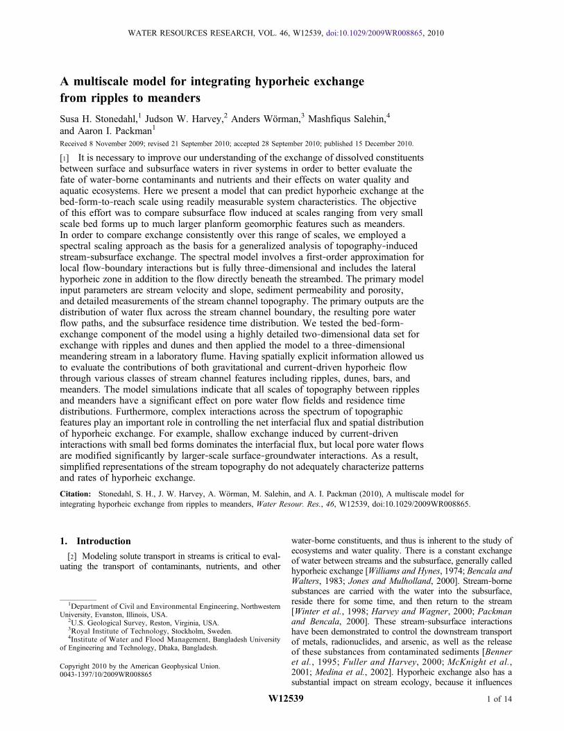
multiple scales of fluvial topography spanning ripples, dunes,alternate bars, and meanders, as illustrated in Figure 1.

2. Modeling Approach

[6] Our approach to modeling surface‐subsurface inter-actions involves three essential steps: calculating the headdistribution on the stream channel boundary, calculating thesubsurface flow field, and evaluating the resulting interfacialfluxes, subsurface flow paths and residence time distribu-tions. A brief overview of the approach is provided here,and details follow in sections 2.1–2.3. The estimation of thehead distribution along the entire stream bottom and sub-merged portion of the banks is critical to the calculationof hyporheic fluxes and residence times. This calculationis challenging because of the very wide variety of topo-graphical features that induce interfacial and pore waterflows. In particular, a key challenge here was to estimate theboundary head distribution along the stream channel withoutusing CFD simulations, which are generally not feasiblefor large, multiscale problems. We developed a model thatincludes gravitational head gradients associated with down-stream elevation changes and an approximate solution forvelocity head gradients induced by the interaction of thestreamflow with the channel boundary. The gravitationalcomponent was obtained directly from the average gradientof the stream over the study reach, obtained from waterelevation measurements, and then head fluctuations due tosmaller topographical features within the stream channelwere superimposed. We approximated the head variationover submerged bed forms by generalizing an available two‐dimensional solution for advective pore water flow underdunes [Elliott and Brooks, 1997a]. We implemented thissolution in 3‐D by employing a Schwarz‐Christoffel con-formal mapping procedure [Zarrati et al., 2005] to create anonorthogonal coordinate system following the curvingstream channel. This method provides consistent resultsregardless of the orientation of the stream, and was used toevaluate the effects of the gravitational head gradient on thethree‐dimensional stream topography as well as the distri-bution of velocity head associated with submerged topo-graphic features within the meandering channel. Effectively,the generalized flow‐boundary interaction model calculatesthe pressure distribution over bed forms relative to the direc-tion and magnitude of the local stream velocity. The interfacialhead distribution over the stream channel boundary wasobtained simply as the sum of the gravitational and velocityhead components. This head distribution was then employedas a boundary condition in a finite difference solution forsubsurface water flow, allowing lateral (floodplain) exchangeand broader stream‐groundwater interactions to be simulatedalong with the local exchange associated with bed forms.The resulting subsurface flow field was then used to evaluateinterfacial fluxes by integrating the local pore water velocityover the bed surface. Hyporheic exchange flow paths andresidence time distributions were also obtained directly fromthe subsurface flow field by means of a numerical particletracking method.

2.1. Representation of Channel Topography

2.1.1. Conformal Mapping[7] The morphology of the meandering channel was trans-

formed into an orthogonal domain using Schwarz‐Christoffel

STONEDAHL ET AL.: A 3‐D FLOW MODEL FOR HYPORHEIC EXCHANGE W12539W12539

2 of 14

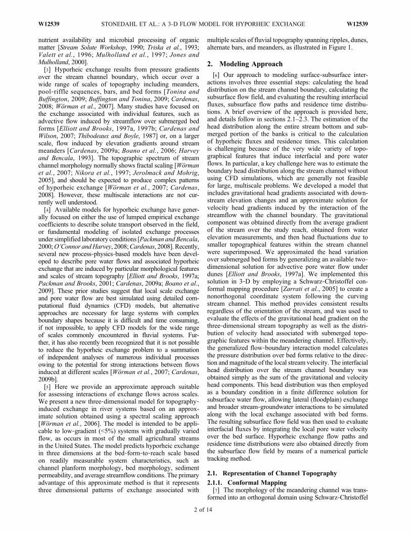
conformal mapping. Conformal mapping preserves localangles while producing a one‐to‐one mapping between dif-ferently shaped domains. A polygonal representation of themeandering stream was mapped onto a rectangle using theSC‐Toolbox for MATLAB [Driscoll, 1996]. This mappingonto a rectangle was found by combining the solution for abi‐infinite strip with a Jacobi elliptic function. The calcula-tion used a Gauss‐Newton method for numerically solvinga system of nonlinear equations. The conformal mapping isillustrated in Figure 2. The longitudinal and transversecoordinates are defined as x and y, while in the transformeddomain these are x and h, respectively.[8] The channel banks were calculated by selecting the

grid points closest to where the stream water surface inter-sected the three dimensional topography grid. The bankswere used to define a polygon, which was formatted intocomplex coordinates with the vertices listed counterclock-wise. This polygon was then transformed into a rectangleusing Driscoll’s algorithm. Characterization of the systemgeometry was facilitated by the conformal mapping. Wecalculated length of the stream by taking the inverse map-ping of 1000 evenly spaced points along the centerline ofthe rectangle in the transformed domain. The sum of thedistances between these corresponding points (x, y) in thestream provides a good approximation of the length ofthe stream

S ¼XN�1

i¼1

ffiffiffiffiffiffiffiffiffiffiffiffiffiffiffiffiffiffiffiffiffiffiffiffiffiffiffiffiffiffiffiffiffiffiffiffiffiffiffiffiffiffiffiffiffiffiffiffiffiffixi � xiþ1ð Þ2þ yi � yiþ1ð Þ2

q¼XN�1

i¼1

D�; ð1Þ

where N is the number of points. The sinuosity of thechannel was then determined as the ratio of the streamlength to the reach length. The width of the stream at eachcross section was found similarly to the length. For thiscalculation, we took the inverse conformal mapping ofpoints along each cross section in the transformed domainand summed the distances between them in the real domain.

These values were then averaged to find the mean width ofthe system. The average depth and cross‐sectional areaswere also calculated similarly using the elevations at eachcross section in the real domain. Discharge was assumed tobe constant throughout the reach, and the cross‐sectionalareas were used to determine how the mean velocity variedas a function of downstream distance.2.1.2. Fourier Fitting[9] A Fourier fitting procedure was used for several

purposes in the model: (1) to generate a continuous functionfor topography in both the real and transformed domains,(2) as a means of separating different scales of topographyby wavelength in the Fourier series, and (3) as a means ofcalculating the boundary head distribution from the topo-graphic distribution and streamflow conditions. A trigono-metric polynomial finite Fourier series, P(x, y), having theform given in equation (2) was used to represent topography.The coefficients were calculated in MATLAB using a three‐dimensional extension of the trigonometric polynomialapproximation method [Fink and Mathews, 1999, chap. 5]

P x; yð Þ ¼ ao2þXMx

jx¼1

XMy

jy¼1

ajx jy cos jxkxxð Þ cos jykyy� ��

þ bjx jy sin jxkxxð Þ cos jykyy� �þ . . . cjx jy cos jxkxxð Þ sin jykyy

� �þ djx jy sin jxkxxð Þ sin jykyy

� ��þXMx

jx¼1

ej cos jxkxxð Þ�

þ fj sin jxkxxð ÞÞ þ . . .XMy

jy¼1

gj cos jykyy� �þ hj sin jykyy

� �� �:

ð2Þ

The angular wave number for each of the terms was theproduct of an integer and the wave number, kx or ky, wherekx = 2p/lx and ky = 2p/ly. lx is both the maximum wave-length and size of the domain in the longitudinal directionand ly is the maximum wavelength and size of the domainin the transverse direction. In equation (2), the wavelengthof each term is an integer fraction of the maximum wave-length. By imposing these restrictions on the selection ofthe angular wave numbers used in the Fourier series, each ofthe resulting wavelengths divides evenly into the domainsize, causing the function to be periodic in both the longi-tudinal and transverse directions. This periodicity is essentialfor the calculation of head variation over small bed formtopography (ripples and dunes), which would otherwisegenerate unrealistic topography outside of the computationaldomain [Wörman et al., 2006]. This condition also made itimportant to start and end the reach at similar locations rela-

Figure 2. Illustration of Schwarz‐Christoffel conformalmapping used to transform the meandering stream with(x, y) coordinates into a rectangle with (x.h) coordinates.

Figure 1. Hyporheic exchange associated with ripples,dunes, bars, and meanders. Reach‐scale patterns of exchangereflect complex interactions between these features andlarger‐scale groundwater discharge/recharge.

STONEDAHL ET AL.: A 3‐D FLOW MODEL FOR HYPORHEIC EXCHANGE W12539W12539

3 of 14

tive to the larger‐scale channel topography, here the apexesof two meanders. In real systems, the topography outside ofthe study reach is generally unknown, so it is reasonable toassume periodicity in the topography before and after thestudy reach. However, this assumption may be inappropriateif stream characteristics show distinct trends in the longitud-inal direction.[10] The accuracy of the fitting procedure depends on the

number of wavelengths used to fit the surface in each direc-tion, Mx and My. Each additional wavelength improves theaccuracy of the Fourier fit, but only up to the maximumaccuracy set by the spatial resolution and quality of theoriginal topographic data. We set Mx and My to be one lessthan half of the number of data points in each direction tocomply with the Nyquist frequency cutoff, correspondingto the maximum information content of the data set. Usingfrequencies greater than the Nyquist cutoff does not provideany additional information and instead induces extraneousfluctuations in the surface, which would yield spurious porewater flows. Unlike previous work [Wörman et al., 2006],which used a limited number of terms in the Fourier seriesused to represent the surface topography, we used all termsup to the Nyquist frequency cutoff, which used the maximuminformation content of the data sets.

2.2. Calculation of the Boundary Head Distribution

[11] It is necessary to calculate the head distribution overlarge and small topographic features separately becauseflow‐boundary interactions produce substantial head gra-dients over steep features such as dunes, but not over largerand smoother features such as meanders. In general, thereis a variation of velocity head over any submerged shape,but particularly large pressure gradients are produced wher-ever there is a flow separation and recirculation. This occursprimarily at bed form crests [Thibodeaux and Boyle, 1987;Elliott and Brooks, 1997a; Cardenas et al., 2008; Cardenas,2008]. Thus, local variations in velocity head over bed formsrepresent important local perturbations to the energy gradeline of the stream. We used an approximate criterion toseparate the bed topography into two classes of features:large topography for which only the mean energy grade lineis used to calculate the boundary head distribution, andsmall topography for which local variability in velocity headis included in the boundary head distribution. We establishedthe cutoff threshold based on the range of applicability of thegradually varied flow equations. In order for the large‐scale

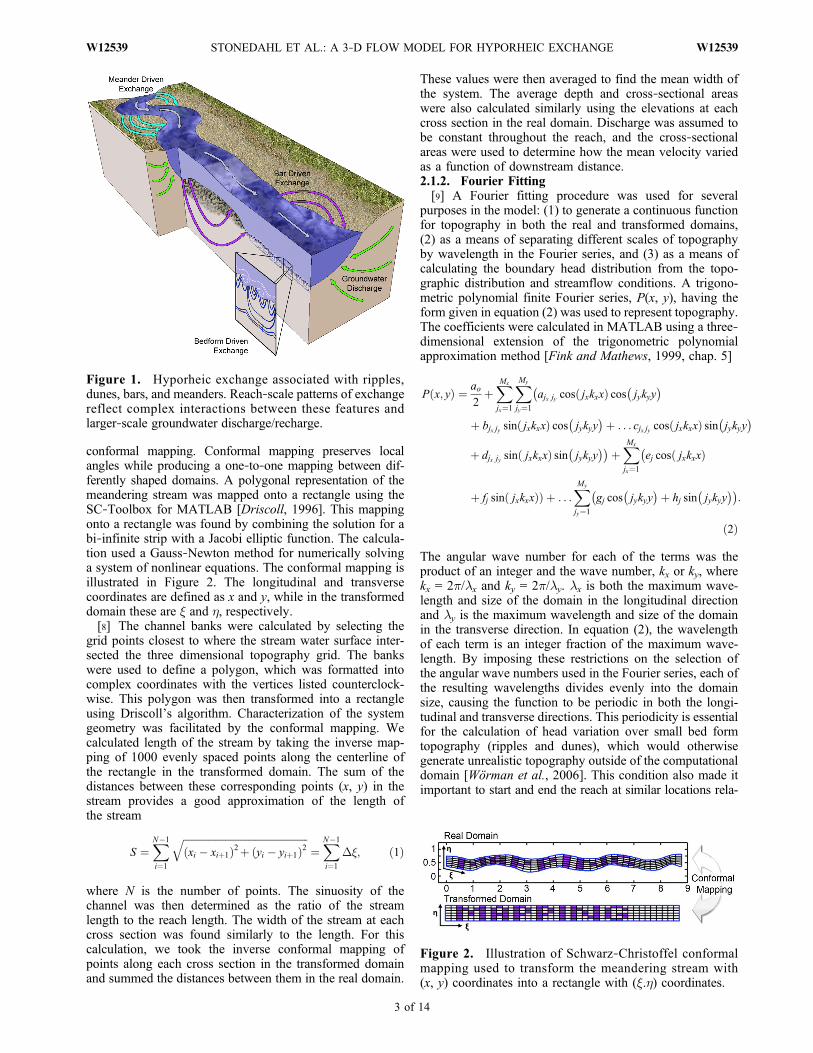
topography to comply with the gradually varied flow equa-tions, the slope must be less than 5% [Chaudhry, 1993], sothe threshold wavelength, lc, was chosen such that all fea-tures identified as large topography have slope no greaterthan 5%. This scale separation provides a further advantagein that it also prevents the generation of spurious headfluctuations over large morphological features with ampli-tudes exceeding the mean flow depth, but over very longwavelengths. The procedures for calculating the boundaryhead distribution over each of these scales of topographicalfeatures are detailed below.2.2.1. Head Distribution Over Large‐Scale Topography[12] The head distribution over large‐scale topographic

features (l > lc) was obtained from the energy grade lineover the reach. It is difficult to measure the elevation of thefree surface precisely, which leads to large errors in theestimation of the hydraulic gradient over small separationdistances. Even for the relatively high‐density laboratorydata sets used here for the initial model application, wefound that the free surface measurements were only sufficientto enable estimation of the mean longitudinal hydraulic slopeof the flume. The constant slope was applied in the trans-formed domain, which is equivalent to applying head valuescorresponding to the slope to each cross section in the realdomain. To illustrate the results of this process, Figure 3shows gravitational head contours within the stream bound-ary for one of our data sets. (The method for calculating thehead contours outside of the stream boundaries is discussedin section 2.3.) Specifically, Figure 3 illustrates how thelinear gradient in the transformed domain follows the streamchannel in the real domain.2.2.2. Small‐Scale Topography Head Distribution[13] Streamflow over small‐scale topographic features pro-

duces regular perturbations in the boundary head distributionthat generate important components of the subsurface flow[Thibodeaux and Boyle, 1987; Elliott and Brooks, 1997a;Cardenas, 2008]. The velocity head perturbation over aripple‐ or dune‐shaped feature is known to be approximatelysinusoidal [Elliott and Brooks, 1997a, 1997b]. We general-ized this solution in two dimensions by representing theboundary head distribution, h1(x), as a sine curve with ascaled amplitude shifted a quarter of a wavelength from thetopography function, t1(x),

t1 xð Þ ¼ H

2sin kxð Þ; ð3Þ

h1 xð Þ ¼ hm sin k xþ �

4

� �; ð4Þ

where hm is the amplitude of the head distribution, H is thebed form height, k is the wave number, l is the wavelength,and x is the longitudinal direction. Using this approach, theboundary head distribution is obtained as a Fourier series,where each term is obtained directly from the Fourier seriesused to represent the streambed topography. Fehlman’s[1985] correlation was used to estimate the amplitude ofthe dynamic head variation for each term

hm ¼ 0:28V 2

2g

� � H=d

0:34

� �3=8

H=d � 0:34

H=d

0:34

� �3=2

H=d � 0:34

8>>><>>>:

; ð5Þ

Figure 3. Gravitational head due to large‐scale features isheld constant for each cross section by applying it in thetransformed coordinate system. Within the stream this showscross sections with uniform gravitational head values, whichare roughly perpendicular to the banks. Outside of the streamchannel the head contours straighten back out and are perpen-dicular to the flume walls by the time the edges are reached.

STONEDAHL ET AL.: A 3‐D FLOW MODEL FOR HYPORHEIC EXCHANGE W12539W12539

4 of 14

where hm is the amplitude of the head perturbation, V is themean velocity of the overlying flow, d is the mean flowdepth, and g is the gravitational constant. This equationhas been shown to work well as an estimator of pore waterflow paths and surface‐subsurface exchange under two‐dimensional bed forms, i.e., regular dunes that span thewidth of the flow [Elliott and Brooks, 1997a], and isextended here to three‐dimensional features. The conformalmapping described above ensures that the sinusoidal headprofile is aligned with the direction of the local streamvelocity, which varies throughout a three‐dimensional streamchannel. In the transformed domain, we Fourier fit a scaledversion of the topography and calculated the velocity headby shifting each component of the Fourier series byone quarter of its wavelength in the negative x direction,following equation (4). This creates an approximate three‐dimensional solution for the boundary head distribution witha region of higher head on the upstream side of each bedform. This model is quasi‐three‐dimensional because wegeneralized the 2‐D solution (equations (3)–(5)) relative tothe local channel planform morphology following the longi-tudinal conformal lines. We expect this approximation to bereasonable given the strongly two‐dimensional nature ofriver flows and dune morphology; however, cases with ahigh degree of cross‐channel variability and/or stronglythree‐dimensional bed forms may not be represented well.[14] Stream velocities, depths, and bed form sizes can be

highly variable such that mean values for the entire reachmay not accurately represent the characteristics of a smallerchannel segment. From equation (5), it can be seen thatfluctuations in the stream depth and velocity associated withslowly varying large‐scale topography affect the estimate ofexchange resulting from local scale flow‐boundary inter-actions. In addition, bed form morphology often variessignificantly within a reach. To account for this variability,we calculated continuous functions of d, V, and H to scalethe velocity head component of the boundary head distri-bution at each point of the stream. The local stream depth d(x) was first calculated as a moving average of the averagedepth for each cross section over a window size lc centeredat x. The elevation perturbation specifically associated withbed forms, "(x), was then calculated by subtracting d(x)from the average depth for each cross section. In previouswork, H has been found from the standard deviation of localbed elevation measurements, sH. Specifically, Elliott andBrooks [1997a, 1997b] used H = 2sH as an approximateaverage bed form height for exchange with a regular series of2‐D dunes. Here, we obtained sH(x) by taking the standarddeviation of points in "(x) over a window size lc centered at x.This extends the model to include slowly varying channelmorphology. For a perfectly sinusoidal topography, s =ffiffiffiffiffiffiffiffiffiffiffiffiffiffiffiffiffiffiffiffiffiffiffiffiffiffiffiffiffiffiffiffiffiffiffiffiffiffiffiffiffiffiffiffiffiffiR2�

0H=2ð Þ sin xð Þ^2� �

=2�

s= H/2

ffiffiffi2

p, yielding 2

ffiffiffi2

ps = H.

Further, for the triangular bed forms used by Elliott as testcases [Elliott and Brooks, 1997b], taking H = 2

ffiffiffi2

ps mat-

ches the measured heights of individual dunes within 3%.Therefore we evaluated the bed form height used inequation (5) as 2

ffiffiffi2

psH(x). The average stream velocity,

V(x, h), varies in both the longitudinal and transverse direc-tions. The mean velocity for each cross section is simply thevolumetric water flux. This was calculated in the model bydividing the discharge (which was constant) by the local

cross‐sectional area (which varied). We included a simplefirst‐order correction to account for the transverse velocityprofile within each cross section by assuming that V is pro-portional to depth. This caused the maximum velocity tooccur in the thalweg and forced V = 0 at the edges of thechannel, which was required to provide a realistic repre-sentation of lateral exchange through the stream banks. Thistransverse variation in the stream velocity created greaterfluctuations in velocity head in the deeper portions of thechannel relative to the surrounding shallow areas, leading totransverse pore water velocity components.[15] The final scaling function for the velocity head per-

turbation over small topography (bed forms) includingspatial variability in velocity, depth, and amplitude is

hm0 �; �ð Þ ¼

0:28V �; �ð Þ2

2g

!ffiffiffi2

p�H �ð Þ

�

2ffiffiffi2

p�H �ð Þ=d �ð Þ0:34

!3=8

2ffiffiffi2

p�H �ð Þ=d �ð Þ � 0:34

2ffiffiffi2

p�H �ð Þ=d �ð Þ0:34

!3=2

2ffiffiffi2

p�H �ð Þ=d �ð Þ � 0:34

8>>>>><>>>>>:

:

ð6Þ

After the topography is multiplied by h′m(x, h), the resultingFourier series for the distribution of velocity head over thestream channel resulting from flow‐boundary interactionsin the transformed domain is

Fh �; �ð Þ ¼ Ao

2þXM�

j�¼1

XM�

j�¼1

Aj� j� cos j�k�� þ 2�

4j�k�

� �cos j�k��� ��

þ Bj� j� sin j�k�� þ 2�

4j�k�

� �cos j�k��� �

þ . . .Cj� j� cos j�k�� þ 2�

4j�k�

� �sin j�k��� �

þDj� j� sin j�k�� þ 2�

4j�k�

� �sin j�k��� ��

þ . . .XM�

j�¼1

Ej cos j�k�� þ 2�

4j�k�

� ��

þ Fj sin j�k�� þ 2�

4j�k�

� ��

þXM�

j�¼1

Gj cos j�k�y� �þ Hj sin j�k��

� �� �; ð7Þ

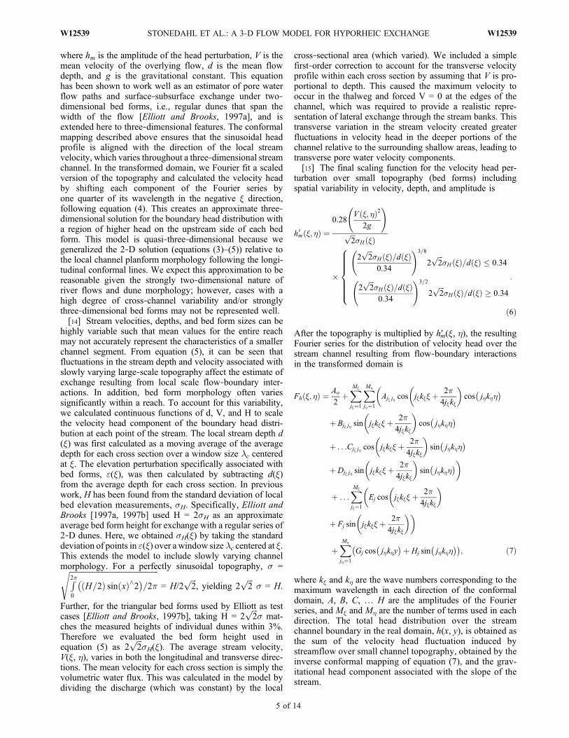
where kx and kh are the wave numbers corresponding to themaximum wavelength in each direction of the conformaldomain, A, B, C, … H are the amplitudes of the Fourierseries, and Mx and Mh are the number of terms used in eachdirection. The total head distribution over the streamchannel boundary in the real domain, h(x, y), is obtained asthe sum of the velocity head fluctuation induced bystreamflow over small channel topography, obtained by theinverse conformal mapping of equation (7), and the grav-itational head component associated with the slope of thestream.

STONEDAHL ET AL.: A 3‐D FLOW MODEL FOR HYPORHEIC EXCHANGE W12539W12539

5 of 14

2.3. Three‐Dimensional Simulation of Subsurface Flow

[16] MODFLOW [Harbaugh et al., 2000] was used tocalculate the three‐dimensional distribution of head andvelocity in the subsurface. For the initial application to flumeexperiments, the entire sedimentary system was includedin the computational domain, as shown in Figure 4. Theupstream and downstream boundaries were defined as con-stant heads, which were set in the flume by the selecteddischarge, the flume geometry, and hydraulic controls at theinlet and outlet. The flume bottom and walls defined no‐flowboundaries. The surface‐subsurface interface was used as aconstant head boundary after the boundary head distributionwas calculated as described in section 2.2. In the three‐dimensional case additional steps were required to calculatethe free surface outside of the stream channel.[17] Pore fluid flow was calculated from the three‐

dimensional subsurface head distribution using Darcy’s law,qs = −Krh1, where qs is the specific discharge, K is thehydraulic conductivity, r is the del operator, and h1 is thehead distribution. We used a constant K because the sedi-ments used in flume experiments were essentially homo-geneous. The seepage velocity or pore velocity, qp, wascalculated from the specific discharge using the porosity, �,qp = qs

� . The interfacial boundary flux, qint = n̂ · qs, wascalculated based on the local value of the Darcy velocity andthe unit normal to the surface, n̂. Measurements of surfacetopography were fit with a discrete Fourier transform inorder to create a differentiable function, which allowed usto easily calculate the normal vector at any point on thestreambed surface.[18] Hyporheic exchange flow paths and subsurface resi-

dence time distributions were determined from the subsur-face flow field by particle tracking. To evaluate exchange,1000 particles were distributed over the streambed surfaceat locations randomly selected from a probability distributionproportional to the boundary influx. Particle motion in thesubsurface was deterministic, as it was calculated basedsolely on the calculated seepage velocity distribution. Dis-persion was neglected because other studies have found thisto have only a small effect on residence times for thehomogeneous sediments and scale of topography includedin this model [Elliott and Brooks, 1997a, 1997b; Salehinet al., 2004]. Particles were tracked through the system

using a constant distance step, DStep, and a variable timestep. The selection of DStep is delicate as smaller values yieldmore accurate results, but also substantially increase theamount of time required to perform particle tracking. In eachiteration, the local seepage velocity was calculated from alinear interpolation of the head distribution at each particlelocation, and each particle was then translated by the distanceDStep in the direction of the seepage velocity. The periodicityimposed on the model domain allowed us to track the fateof particles that reached the downstream boundary simplyby reintroducing them into the domain at the correspondinglocation of the upstream boundary. The location of each par-ticle was tracked relative to the streambed surface at every stepin the particle‐tracking routine. The subsurface residence timedistribution was calculated simply by recording the amountof time that each tracked particle took to return to the surfacewater. The resulting residence time distribution was fluxweighted because the particles were introduced to the sub-surface in proportion to the boundary flux.

3. Model Testing and Application

[19] Two laboratory data sets are used here to illustratethe functionality of the approach and to explore patterns andrates of hyporheic exchange over the bed‐form‐to‐reachscale. First, we simulate exchange with a regular series ofessentially two‐dimensional dunes in a laboratory flume.The topographic information for this case consists of finelyspaced topographic data along the centerline of the channel.Modeling this 2‐D case did not require a conformal map-ping of the head boundary condition, but it did use the headcalculation from the Fourier decomposition, interfacial fluxcalculation, and particle tracking procedure. This experi-ment also included observations of solute exchange with thebed, which we compare against the model simulations inorder to evaluate the Fourier series exchange model for aspectrum of 2‐D topography. Second, we simulate exchangein a naturally meandering channel generated in a relativelywide flume. No measurements of solute transport are avail-able for this second data set, but it is included here becausethe highly detailed observations of 3‐D stream topographyallow us to investigate the interplay of exchange between bedforms and meanders.

3.1. Exchange With Dunes and Ripples

3.1.1. Experiment Setup[20] A recirculating flume, which allowed for sediment

transport, was used for this experiment. It was 12 m long,26.5 cm wide, 25.4 cm deep. The flume contained high‐purity silica sand (Ottawa 3.0) with a geometric meandiameter of 480 microns. The sand had a porosity of 0.33and a hydraulic conductivity of 9 cm/min at an averagebed depth was 10.5 cm. Bed topography was generatednaturally by sediment transport under a uniform overlyingflow 9.8 cm deep and having a mean velocity of ∼25 cm/s.This led to the formation of a series of dunes and ripples thatwere nearly two‐dimensional, generally spanning the widthof the channel but with some irregularity in the shaperesulting from the relatively narrow flume. After the bedtopography was established, the stream discharge and slopewere decreased until there was no bed sediment transport,and then the solute injection experiment was performedunder steady uniform flow conditions. During the solute

Figure 4. Boundary conditions of the modeling domainfor the finite difference calculation. The bottom and wallsof the flume are no flow boundaries. The upstream anddownstream boundaries are constant heads given by thevalues of the head in the surface layer. The surface layeris found during an intermediate two‐dimensional calculationand is held constant for the three‐dimensional calculation.

STONEDAHL ET AL.: A 3‐D FLOW MODEL FOR HYPORHEIC EXCHANGE W12539W12539

6 of 14

injection, the average stream depth was 9.8 cm, the meanvelocity was 16.7 cm/s, and the slope was 0.00022. Lithiumwas used as the conservative tracer. A solution of lithiumchloride was added to the flume to establish a uniform initialconcentration of C0 = 38.9 mM in the stream water. Surface‐subsurface exchange caused the in‐stream concentration todecrease over time owing to mixing (dilution) with tracer‐free pore water. The primary solute transport is thus a timeseries of measurements of the in‐stream lithium concentra-tion, obtained by ICP‐MS (Perkin‐Elmer Elan 5000). Theinitial concentration is used to normalize all of the latersolute measurements.[21] The bed form topography was characterized using a

laser profiler (Keyence LD‐1101), which provided a seriesof high‐resolution bed surface elevation measurementsalong the centerline of the flume. The laser profiling providesmore detailed information on smaller‐scale topographicalfeatures, like ripples, than can be obtained by visual oracoustic measurements, making this an excellent data setfor model application and testing. This device was mountedon flume rails and driven by a stepper motor. Reflectionsdue to the water surface were avoided by mounting the laserin a waterproof box with a glass bottom, which was loweredinto the stream. Point elevation measurements were madeevery 9.1 mm and have a precision of ∼10 mm. The topog-raphy data set consists of 588 evenly spaced points, whichspanned a distance of 5.33 m.3.1.2. Simulations and Results[22] We used the model described in section 2 to predict

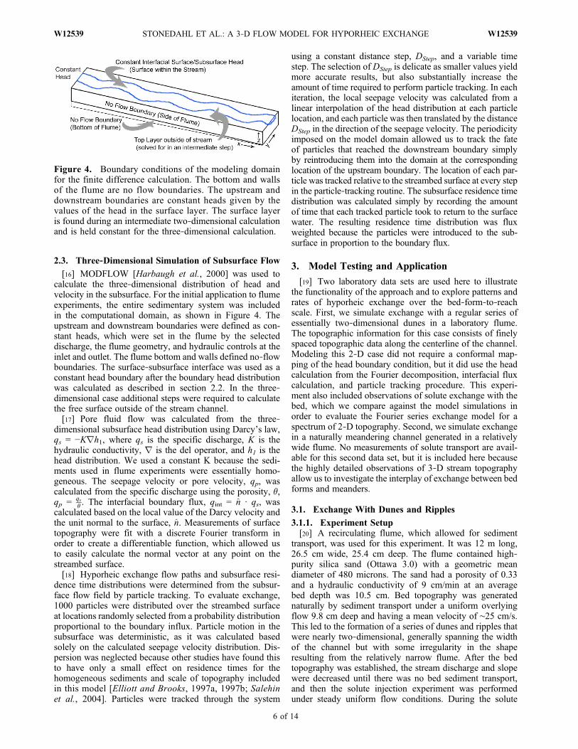
pore water flow paths and solute exchange in this experi-ment. The subsurface model domain consisted of a 1762 ×83 × 17 grid. Particles were tracked through this system witha constant DStep = 10−5 m. The results were compared withthe measured solute concentration data. The calculatedboundary head over the two‐dimensional topography andhyporheic exchange streamlines are shown in Figure 5 (left).These results clearly demonstrate the correspondence betweentopography and head, as well as the location of the maxi-mum head upstream of the bed form crests. Calculated flowpaths qualitatively match flow patterns commonly observed

in dye tracer experiments in flumes [Elliott and Brooks,1997b]. However, in contrast to previous models that useonly a single representative scale of topography, the stream-lines can be seen to reflect the multiple scales of topographyfound in this system.[23] We used the approach of Elliott and Brooks [1997a,

1997b] to predict the change in in‐stream concentrationfrom the simulated boundary exchange flux and subsurfaceresidence time distribution. This involved numerically solv-ing the following convolution integral:

C tð ÞCo

¼ 1� q

d0C0

Z t

0R �ð ÞC t � �ð Þd�; ð8Þ

where overbars indicate spatial average over the streambed,C(t) is the in‐stream concentration, q is the spatially averagedinterfacial flux, d′ is the effective stream depth: the ratiobetween the total volume of stream water and the surface areaof the sediment bed, R(t) is the flux‐weighted cumulativeresidence time distribution, t is the time since the solute wasadded to the system, and t is the time at which solute enteredthe subsurface. The predicted and observed time series ofnormalized in‐stream tracer concentrations are presented inFigure 5 (right). The predicted concentrations match theshape of the curve and reproduce the measured values with anaverage error of 2.0% and a maximum error of 3.2%. Theinterfacial flux can be calculated directly from the initialslope of the C(t) curve, q = d′(DC(t)/C0Dt). The observedinterfacial flux was 5.07E‐6 m/s, whereas the flux predictedby the model was 6.24E‐6 m/s, corresponding to an error of19%. These results show that the model provides a reason-able first‐order approximation for hyporheic exchange undercomplex streambed topography.

3.2. Exchange With a Meandering Channel

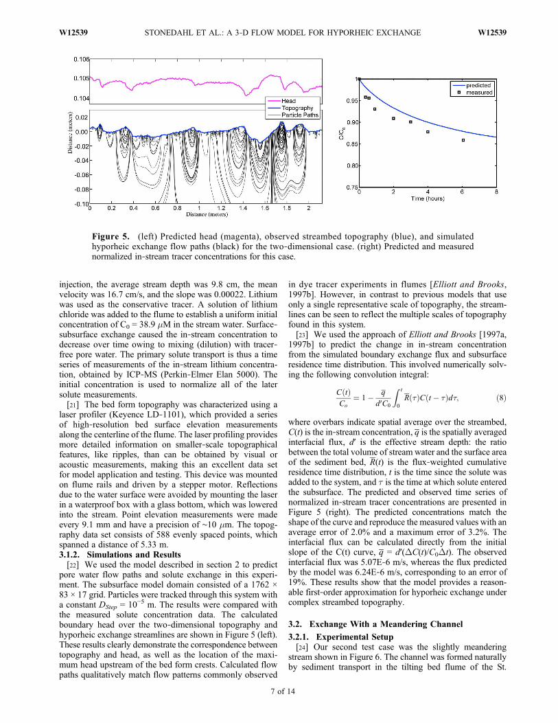
3.2.1. Experimental Setup[24] Our second test case was the slightly meandering

stream shown in Figure 6. The channel was formed naturallyby sediment transport in the tilting bed flume of the St.

Figure 5. (left) Predicted head (magenta), observed streambed topography (blue), and simulatedhyporheic exchange flow paths (black) for the two‐dimensional case. (right) Predicted and measurednormalized in‐stream tracer concentrations for this case.

STONEDAHL ET AL.: A 3‐D FLOW MODEL FOR HYPORHEIC EXCHANGE W12539W12539

7 of 14

Anthony Falls Laboratory (SAFL), University of Minnesota.The flume, shown in Figure 6, was 14.6 m long, 0.9 m wideand 0.6 m deep. The upstream end of the flume had a 1.9 mlong by 0.9 m wide head box, which provided smooth anduniform entry of water into the test section. The mainchannel test section included a 12 m long sediment bed. Thewater depth and discharge in the flume were controlled by atailgate at the downstream end. Uniform flow was obtainedby adjusting the slope and tailgate height to match theaverage energy grade line for the imposed discharge, bedsediments, and emergent bed morphology. The flume wascontinuously supplied with river water during the formationof the channel. All experiments were performed with NelsonSafety Grit sand (Nelson Quarry, Ontario, Canada) withd50 = 1.0 mm. The sediment had a relatively narrow sizedistribution, with 90% having a diameter finer than 3 mm,30% finer than 0.8 mm and only 3% finer than 0.3 mm. Theporosity, �, of the sediment was measured and found to be0.37. The hydraulic conductivity, K, was measured using aconstant head permeameter and found to be 0.11 cm/s.[25] The meandering channel was formed by cutting a

straight trapezoidal channel of W = 35 cm, d = 4 cm in thesediment bed, with half of a meander bend included at theupstream end of the flume (following Olsen [2003]). Waterwas supplied at bank‐full depth, a velocity of 50 cm/s,and channel slope (Ss) of 0.007. Flow around the initialmeander bend led to the formation of a series of meanders.During this period of channel formation, sediments weresupplied at the upstream end of the flume by a sedimentfeeder (Accurate, model 580–353600A). The meanderswere allowed to grow until they approached the channelwalls after approximately 4 h, at which point the slope anddischarge were reduced until sediment transport ceased,leaving relict channel and bed form topography.[26] The resulting meandering channel had four well‐

defined meander bends with an average wavelength of2.20 m and average amplitude of 0.08 m. The topographyof the meandering channel was measured with a sonartransit system mounted on a three‐dimensional positioninginstrument carriage that traversed the length of the flume.The bed profile was measured along 16 longitudinal trans-ects evenly spaced across the channel width, with 136 reg-ularly spaced elevation measurements along each transect.

The average curvature of the stream was 0.43 m−1, yieldingan average radius of curvature of 2.3 m and a sinuosity of1.01. The ratio of the radius of curvature to the stream widthwas thus 5.7. Variations in depth were relatively small anduniform within the meanders. Uniform streamflow throughthis meandering channel was observed to have an energygrade line slope of 0.0013, a mean depth of 3.8 cm, and amean velocity of 16 cm/s.[27] This channel morphology represents a case of incipi-

ent meandering. Much greater sinuosity can be found innature, but this laboratory‐generated meandering channel is auseful test case for initial application of the 3‐D exchangemodel because the stream morphology was characterizedin detail, the underlying sediments were homogeneous, andthe hydraulic conductivity, porosity, and streamflow condi-tions were known precisely. Unfortunately no solute injec-tion results are available for this case, but the high‐qualityobservations of channel topography, sediment properties, andstreamflow still make this a useful data set.3.2.2. Simulations and Results[28] For the three‐dimensional simulation, we modeled

the entire sediment bed under and around the four meanders,out to the channel walls. The side and bottom planes weredefined as no‐flow boundaries, corresponding to the side-walls and bottom of the flume, respectively. The top surfaceof the domain includes the meandering stream channeland extends to the flume walls. Head values at the stream‐subsurface interface were assigned according to the Fouriermodel described in section 3.2.1. The free surface outside ofthe stream was calculated using a separate MODFLOWsimulation on an unconfined two‐dimensional grid, basedon the calculated head distribution within the stream channeland no‐flow boundaries at the channel walls. The resultinghead surface was then used as the top boundary outside thestream channel in the 3‐D MODFLOW simulation. Notethat the heads inside and outside the stream channel matchexactly at the limit of the stream banks even when thevelocity head is included within the stream because V → 0along the line of contact.[29] We created a grid 17 layers deep with a higher

density of layers near the surface in order to better resolveshallow hyporheic exchange flow paths. The top layer was0.0002 m thick, each subsequent layer increased in thick-ness by a factor of 1.5, and a thin bottom layer (0.002 m)was included to improve the simulation of flow paths thatapproached this no‐flow boundary. The grid was composedof 676 × 96 × 17 cells and DStep = 0.001 m. We confirmedthat this value of DStep was sufficiently small so as not toaffect the results. We represented the banks of the mean-dering channel using a 272‐point polygon. The topographydata set consists of an 136 × 16 orthogonal grid. The streamchannel boundaries were defined from these measuredvalues as described in section 2.2. The limited resolution ofthe topographic measurements caused the initial estimates ofthe stream bank to be rough, so we smoothed the banksusing a moving average with a 26 cm window, therebyeliminating truly local edge anomalies.[30] We ran multiple simulations of hyporheic exchange,

including not only the full observed system complexity,but also simplified representations of the system. We usedsmoothed and idealized representations of the channel topog-raphy to evaluate how various scales of topography affectboundary fluxes and subsurface residence time distributions.

Figure 6. Meandering channel in a tilting flume.

STONEDAHL ET AL.: A 3‐D FLOW MODEL FOR HYPORHEIC EXCHANGE W12539W12539

8 of 14

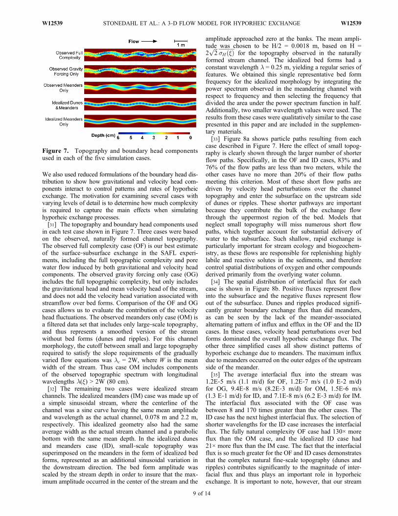
We also used reduced formulations of the boundary head dis-tribution to show how gravitational and velocity head com-ponents interact to control patterns and rates of hyporheicexchange. The motivation for examining several cases withvarying levels of detail is to determine how much complexityis required to capture the main effects when simulatinghyporheic exchange processes.[31] The topography and boundary head components used

in each test case shown in Figure 7. Three cases were basedon the observed, naturally formed channel topography.The observed full complexity case (OF) is our best estimateof the surface‐subsurface exchange in the SAFL experi-ments, including the full topographic complexity and porewater flow induced by both gravitational and velocity headcomponents. The observed gravity forcing only case (OG)includes the full topographic complexity, but only includesthe gravitational head and mean velocity head of the stream,and does not add the velocity head variation associated withstreamflow over bed forms. Comparison of the OF and OGcases allows us to evaluate the contribution of the velocityhead fluctuations. The observed meanders only case (OM) isa filtered data set that includes only large‐scale topography,and thus represents a smoothed version of the streamwithout bed forms (dunes and ripples). For this channelmorphology, the cutoff between small and large topographyrequired to satisfy the slope requirements of the graduallyvaried flow equations was lc = 2W, where W is the meanwidth of the stream. Thus case OM includes componentsof the observed topographic spectrum with longitudinalwavelengths l(x) > 2W (80 cm).[32] The remaining two cases were idealized stream

channels. The idealized meanders (IM) case was made up ofa simple sinusoidal stream, where the centerline of thechannel was a sine curve having the same mean amplitudeand wavelength as the actual channel, 0.078 m and 2.2 m,respectively. This idealized geometry also had the sameaverage width as the actual stream channel and a parabolicbottom with the same mean depth. In the idealized dunesand meanders case (ID), small‐scale topography wassuperimposed on the meanders in the form of idealized bedforms, represented as an additional sinusoidal variation inthe downstream direction. The bed form amplitude wasscaled by the stream depth in order to insure that the max-imum amplitude occurred in the center of the stream and the

amplitude approached zero at the banks. The mean ampli-tude was chosen to be H/2 = 0.0018 m, based on H =2ffiffiffi2

p�H �ð Þ for the topography observed in the naturally

formed stream channel. The idealized bed forms had aconstant wavelength l = 0.25 m, yielding a regular series offeatures. We obtained this single representative bed formfrequency for the idealized morphology by integrating thepower spectrum observed in the meandering channel withrespect to frequency and then selecting the frequency thatdivided the area under the power spectrum function in half.Additionally, two smaller wavelength values were used. Theresults from these cases were qualitatively similar to the casepresented in this paper and are included in the supplemen-tary materials.[33] Figure 8a shows particle paths resulting from each

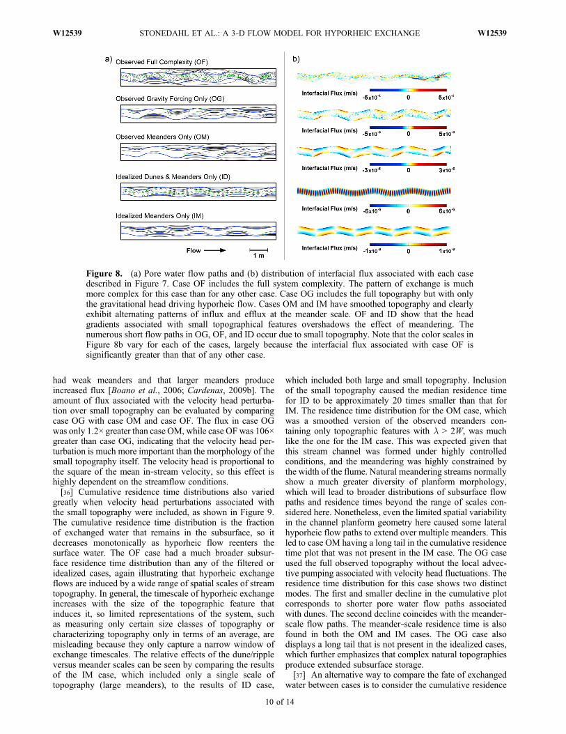
case described in Figure 7. Here the effect of small topog-raphy is clearly shown through the larger number of shorterflow paths. Specifically, in the OF and ID cases, 83% and76% of the flow paths are less than two meters, while theother cases have no more than 20% of their flow pathsmeeting this criterion. Most of these short flow paths aredriven by velocity head perturbations over the channeltopography and enter the subsurface on the upstream sideof dunes or ripples. These shorter pathways are importantbecause they contribute the bulk of the exchange flowthrough the uppermost region of the bed. Models thatneglect small topography will miss numerous short flowpaths, which together account for substantial delivery ofwater to the subsurface. Such shallow, rapid exchange isparticularly important for stream ecology and biogeochem-istry, as these flows are responsible for replenishing highlylabile and reactive solutes in the sediments, and thereforecontrol spatial distributions of oxygen and other compoundsderived primarily from the overlying water column.[34] The spatial distribution of interfacial flux for each

case is shown in Figure 8b. Positive fluxes represent flowinto the subsurface and the negative fluxes represent flowout of the subsurface. Dunes and ripples produced signifi-cantly greater boundary exchange flux than did meanders,as can be seen by the lack of the meander‐associatedalternating pattern of influx and efflux in the OF and the IDcases. In these cases, velocity head perturbations over bedforms dominated the overall hyporheic exchange flux. Theother three simplified cases all show distinct patterns ofhyporheic exchange due to meanders. The maximum influxdue to meanders occurred on the outer edges of the upstreamside of the meander.[35] The average interfacial flux into the stream was

1.2E‐5 m/s (1.1 m/d) for OF, 1.2E‐7 m/s (1.0 E‐2 m/d)for OG, 9.4E‐8 m/s (8.2E‐3 m/d) for OM, 1.5E‐6 m/s(1.3 E‐1 m/d) for ID, and 7.1E‐8 m/s (6.2 E‐3 m/d) for IM.The interfacial flux associated with the OF case wasbetween 8 and 170 times greater than the other cases. TheID case has the next highest interfacial flux. The selection ofshorter wavelengths for the ID case increases the interfacialflux. The fully natural complexity OF case had 130× moreflux than the OM case, and the idealized ID case had21× more flux than the IM case. The fact that the interfacialflux is so much greater for the OF and ID cases demonstratesthat the complex natural fine‐scale topography (dunes andripples) contributes significantly to the magnitude of inter-facial flux and thus plays an important role in hyporheicexchange. It is important to note, however, that our stream

Figure 7. Topography and boundary head componentsused in each of the five simulation cases.

STONEDAHL ET AL.: A 3‐D FLOW MODEL FOR HYPORHEIC EXCHANGE W12539W12539

9 of 14

had weak meanders and that larger meanders produceincreased flux [Boano et al., 2006; Cardenas, 2009b]. Theamount of flux associated with the velocity head perturba-tion over small topography can be evaluated by comparingcase OG with case OM and case OF. The flux in case OGwas only 1.2× greater than case OM, while case OF was 106×greater than case OG, indicating that the velocity head per-turbation is much more important than the morphology of thesmall topography itself. The velocity head is proportional tothe square of the mean in‐stream velocity, so this effect ishighly dependent on the streamflow conditions.[36] Cumulative residence time distributions also varied

greatly when velocity head perturbations associated withthe small topography were included, as shown in Figure 9.The cumulative residence time distribution is the fractionof exchanged water that remains in the subsurface, so itdecreases monotonically as hyporheic flow reenters thesurface water. The OF case had a much broader subsur-face residence time distribution than any of the filtered oridealized cases, again illustrating that hyporheic exchangeflows are induced by a wide range of spatial scales of streamtopography. In general, the timescale of hyporheic exchangeincreases with the size of the topographic feature thatinduces it, so limited representations of the system, suchas measuring only certain size classes of topography orcharacterizing topography only in terms of an average, aremisleading because they only capture a narrow window ofexchange timescales. The relative effects of the dune/rippleversus meander scales can be seen by comparing the resultsof the IM case, which included only a single scale oftopography (large meanders), to the results of ID case,

which included both large and small topography. Inclusionof the small topography caused the median residence timefor ID to be approximately 20 times smaller than that forIM. The residence time distribution for the OM case, whichwas a smoothed version of the observed meanders con-taining only topographic features with l > 2W, was muchlike the one for the IM case. This was expected given thatthis stream channel was formed under highly controlledconditions, and the meandering was highly constrained bythe width of the flume. Natural meandering streams normallyshow a much greater diversity of planform morphology,which will lead to broader distributions of subsurface flowpaths and residence times beyond the range of scales con-sidered here. Nonetheless, even the limited spatial variabilityin the channel planform geometry here caused some lateralhyporheic flow paths to extend over multiple meanders. Thisled to case OM having a long tail in the cumulative residencetime plot that was not present in the IM case. The OG caseused the full observed topography without the local advec-tive pumping associated with velocity head fluctuations. Theresidence time distribution for this case shows two distinctmodes. The first and smaller decline in the cumulative plotcorresponds to shorter pore water flow paths associatedwith dunes. The second decline coincides with the meander‐scale flow paths. The meander‐scale residence time is alsofound in both the OM and IM cases. The OG case alsodisplays a long tail that is not present in the idealized cases,which further emphasizes that complex natural topographiesproduce extended subsurface storage.[37] An alternative way to compare the fate of exchanged

water between cases is to consider the cumulative residence

Figure 8. (a) Pore water flow paths and (b) distribution of interfacial flux associated with each casedescribed in Figure 7. Case OF includes the full system complexity. The pattern of exchange is muchmore complex for this case than for any other case. Case OG includes the full topography but with onlythe gravitational head driving hyporheic flow. Cases OM and IM have smoothed topography and clearlyexhibit alternating patterns of influx and efflux at the meander scale. OF and ID show that the headgradients associated with small topographical features overshadows the effect of meandering. Thenumerous short flow paths in OG, OF, and ID occur due to small topography. Note that the color scales inFigure 8b vary for each of the cases, largely because the interfacial flux associated with case OF issignificantly greater than that of any other case.

STONEDAHL ET AL.: A 3‐D FLOW MODEL FOR HYPORHEIC EXCHANGE W12539W12539

10 of 14

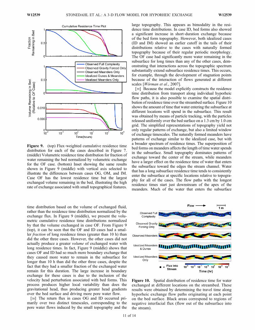
time distribution based on the volume of exchanged fluid,rather than the residence time distribution normalized by theexchange flux. In Figure 9 (middle), we present the volu-metric cumulative residence time distributions normalizedby that the volume exchanged in case OF. From Figure 9(top), it can be seen that the OF and ID cases had a smal-ler fraction of long residence times (greater than 10 h) thandid the other three cases. However, the other cases did notactually produce a greater volume of exchanged water withlong residence times. In fact, Figure 9 (middle) shows thatcases OF and ID had so much more boundary exchange thatthey caused more water to remain in the subsurface forlonger than 10 h than did the other three cases, despite thefact that they had a smaller fraction of the exchanged waterremain for this duration. The large increase in boundaryexchange for these cases is due to the inclusion of thevelocity head perturbation associated with bed forms. Thisprocess produces higher local variability than does thegravitational head, thus producing greater head gradientsover the bed surface and driving more pore water flow.[38] The return flux in cases OG and ID occurred pri-

marily over two distinct timescales, corresponding to thepore water flows induced by the small topography and the

large topography. This appears as bimodality in the resi-dence time distributions. In case ID, bed forms also showeda significant increase in short‐duration exchange becauseof the bed form topography. However, both idealized cases(ID and IM) showed an earlier cutoff in the tails of theirdistributions relative to the cases with naturally formedtopography because of their regular periodic morphology.The OF case had significantly more water remaining in thesubsurface for long times than any of the other cases, dem-onstrating that interactions across the topographic spectrumsubstantially extend subsurface residence times. This occurs,for example, through the development of stagnation pointsbecause of the interaction of flows generated at differentscales [Wörman et al., 2007].[39] Because the model explicitly constructs the residence

time distribution from transport along individual hyporheicflow paths, it is also possible to examine the spatial distri-bution of residence time over the streambed surface. Figure 10shows the amount of time that water entering the subsurface atdifferent locations will spend in the subsurface. This resultwas obtained by means of particle tracking, with the particlesreleased uniformly over the bed surface on a 1.3 cm by 1.0 cmgrid. The simplified representations of topography yield notonly regular patterns of exchange, but also a limited windowof exchange timescales. The naturally formed meanders havepatterns of exchange similar to the idealized case, but witha broader spectrum of residence times. The superposition ofbed forms onmeanders affects the length of time water spendsin the subsurface. Small topography dominates patterns ofexchange toward the center of the stream, while meandershave a larger effect on the residence time of water that entersthe subsurface toward the edges the stream channel. Waterthat has a long subsurface residence time tends to consistentlyenter the subsurface at specific locations relative to topogra-phy for all of the cases. The flow paths with the longestresidence times start just downstream of the apex of themeanders. Much of the water that enters the subsurface

Figure 9. (top) Flux‐weighted cumulative residence timedistribution for each of the cases described in Figure 7.(middle) Volumetric residence time distribution for fraction ofwater remaining the bed normalized by volumetric exchangefor the OF case. (bottom) Inset showing the same resultsshown in Figure 9 (middle) with vertical axis selected toillustrate the differences between cases OG, OM, and IM.Case OF has the lowest residence time but the largestexchanged volume remaining in the bed, illustrating the highrate of exchange associated with small topographical features.

Figure 10. Spatial distribution of residence time for waterexchanged at different locations on the streambed. Theseresults were obtained by determining the travel time alonghyporheic exchange flow paths originating at each pointon the bed surface. Black areas correspond to regions ofnegative interfacial flux (flow out of the subsurface intothe stream).

STONEDAHL ET AL.: A 3‐D FLOW MODEL FOR HYPORHEIC EXCHANGE W12539W12539

11 of 14

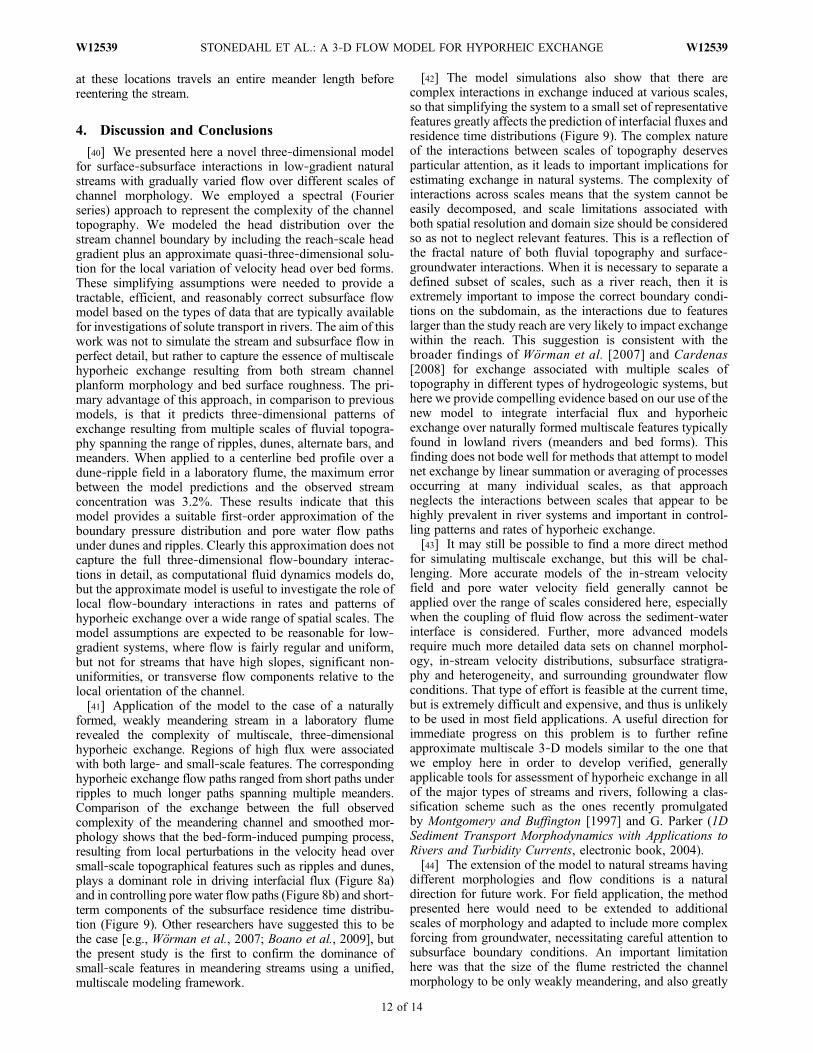
at these locations travels an entire meander length beforereentering the stream.

4. Discussion and Conclusions

[40] We presented here a novel three‐dimensional modelfor surface‐subsurface interactions in low‐gradient naturalstreams with gradually varied flow over different scales ofchannel morphology. We employed a spectral (Fourierseries) approach to represent the complexity of the channeltopography. We modeled the head distribution over thestream channel boundary by including the reach‐scale headgradient plus an approximate quasi‐three‐dimensional solu-tion for the local variation of velocity head over bed forms.These simplifying assumptions were needed to provide atractable, efficient, and reasonably correct subsurface flowmodel based on the types of data that are typically availablefor investigations of solute transport in rivers. The aim of thiswork was not to simulate the stream and subsurface flow inperfect detail, but rather to capture the essence of multiscalehyporheic exchange resulting from both stream channelplanform morphology and bed surface roughness. The pri-mary advantage of this approach, in comparison to previousmodels, is that it predicts three‐dimensional patterns ofexchange resulting from multiple scales of fluvial topogra-phy spanning the range of ripples, dunes, alternate bars, andmeanders. When applied to a centerline bed profile over adune‐ripple field in a laboratory flume, the maximum errorbetween the model predictions and the observed streamconcentration was 3.2%. These results indicate that thismodel provides a suitable first‐order approximation of theboundary pressure distribution and pore water flow pathsunder dunes and ripples. Clearly this approximation does notcapture the full three‐dimensional flow‐boundary interac-tions in detail, as computational fluid dynamics models do,but the approximate model is useful to investigate the role oflocal flow‐boundary interactions in rates and patterns ofhyporheic exchange over a wide range of spatial scales. Themodel assumptions are expected to be reasonable for low‐gradient systems, where flow is fairly regular and uniform,but not for streams that have high slopes, significant non-uniformities, or transverse flow components relative to thelocal orientation of the channel.[41] Application of the model to the case of a naturally

formed, weakly meandering stream in a laboratory flumerevealed the complexity of multiscale, three‐dimensionalhyporheic exchange. Regions of high flux were associatedwith both large‐ and small‐scale features. The correspondinghyporheic exchange flow paths ranged from short paths underripples to much longer paths spanning multiple meanders.Comparison of the exchange between the full observedcomplexity of the meandering channel and smoothed mor-phology shows that the bed‐form‐induced pumping process,resulting from local perturbations in the velocity head oversmall‐scale topographical features such as ripples and dunes,plays a dominant role in driving interfacial flux (Figure 8a)and in controlling pore water flow paths (Figure 8b) and short‐term components of the subsurface residence time distribu-tion (Figure 9). Other researchers have suggested this to bethe case [e.g., Wörman et al., 2007; Boano et al., 2009], butthe present study is the first to confirm the dominance ofsmall‐scale features in meandering streams using a unified,multiscale modeling framework.

[42] The model simulations also show that there arecomplex interactions in exchange induced at various scales,so that simplifying the system to a small set of representativefeatures greatly affects the prediction of interfacial fluxes andresidence time distributions (Figure 9). The complex natureof the interactions between scales of topography deservesparticular attention, as it leads to important implications forestimating exchange in natural systems. The complexity ofinteractions across scales means that the system cannot beeasily decomposed, and scale limitations associated withboth spatial resolution and domain size should be consideredso as not to neglect relevant features. This is a reflection ofthe fractal nature of both fluvial topography and surface‐groundwater interactions. When it is necessary to separate adefined subset of scales, such as a river reach, then it isextremely important to impose the correct boundary condi-tions on the subdomain, as the interactions due to featureslarger than the study reach are very likely to impact exchangewithin the reach. This suggestion is consistent with thebroader findings of Wörman et al. [2007] and Cardenas[2008] for exchange associated with multiple scales oftopography in different types of hydrogeologic systems, buthere we provide compelling evidence based on our use of thenew model to integrate interfacial flux and hyporheicexchange over naturally formed multiscale features typicallyfound in lowland rivers (meanders and bed forms). Thisfinding does not bode well for methods that attempt to modelnet exchange by linear summation or averaging of processesoccurring at many individual scales, as that approachneglects the interactions between scales that appear to behighly prevalent in river systems and important in control-ling patterns and rates of hyporheic exchange.[43] It may still be possible to find a more direct method

for simulating multiscale exchange, but this will be chal-lenging. More accurate models of the in‐stream velocityfield and pore water velocity field generally cannot beapplied over the range of scales considered here, especiallywhen the coupling of fluid flow across the sediment‐waterinterface is considered. Further, more advanced modelsrequire much more detailed data sets on channel morphol-ogy, in‐stream velocity distributions, subsurface stratigra-phy and heterogeneity, and surrounding groundwater flowconditions. That type of effort is feasible at the current time,but is extremely difficult and expensive, and thus is unlikelyto be used in most field applications. A useful direction forimmediate progress on this problem is to further refineapproximate multiscale 3‐D models similar to the one thatwe employ here in order to develop verified, generallyapplicable tools for assessment of hyporheic exchange in allof the major types of streams and rivers, following a clas-sification scheme such as the ones recently promulgatedby Montgomery and Buffington [1997] and G. Parker (1DSediment Transport Morphodynamics with Applications toRivers and Turbidity Currents, electronic book, 2004).[44] The extension of the model to natural streams having

different morphologies and flow conditions is a naturaldirection for future work. For field application, the methodpresented here would need to be extended to additionalscales of morphology and adapted to include more complexforcing from groundwater, necessitating careful attention tosubsurface boundary conditions. An important limitationhere was that the size of the flume restricted the channelmorphology to be only weakly meandering, and also greatly

STONEDAHL ET AL.: A 3‐D FLOW MODEL FOR HYPORHEIC EXCHANGE W12539W12539

12 of 14

restricted the lateral extent of the meander‐induced hyporheicflow paths. Thus, the size of the flume placed a sharp cutoffon the maximum scale of fluvial topography and also on themaximum scale of subsurface flow paths and residence times.The basic behavior found here is expected to extend acrossthe entire topographic spectrum found in rivers, but willbe subject to natural scale cutoffs associated with varioustypes of channel formation processes [Jerolmack et al., 2004;Nikora et al., 1997] and the underlying hydrogeologicstructure [Marklund and Wörman, 2010; Salehin et al., 2004;Packman et al., 2006; Cardenas et al., 2004; Sawyer andCardenas, 2009]. Larger‐scale groundwater flow patternsare expected to influence rates and patterns of hyporheicexchange [Wörman et al., 2007; Cardenas, 2008], so themodel boundary conditions need to include the groundwaterflow field surrounding the stream of interest.[45] Current investigations of solute transport in rivers,

particularly investigations focused on stream ecology andbiogeochemistry, typically do not obtain regular, high‐densitymeasurements of channel morphology, essential hydrogeo-logical properties such as permeability, or any informationon groundwater levels outside the stream channel. It isimportant to realize that the ability to resolve multiple scalesof hyporheic exchange depends directly on the effort put

into characterizing system morphology, sediment properties,and overall surface and groundwater flow conditions. Further,the occurrence of strong, complex interactions across scalesalso implies that even local scale exchange will be highlyinfluenced by processes occurring at the scale of the streamchannel bars and meanders or even the regional groundwaterflow field. Thus, valid quantitative predictions of surface‐subsurface solute transport and effects on related biogeo-chemical processes (rates of oxygen consumption andcycling of nutrients and carbon, and fate of contaminants) arelikely to be much improved with additional effort in char-acterizing channel geometry and flow variability, hydraulicconductitivity, and interactions with groundwater surround-ing the stream.

Appendix A

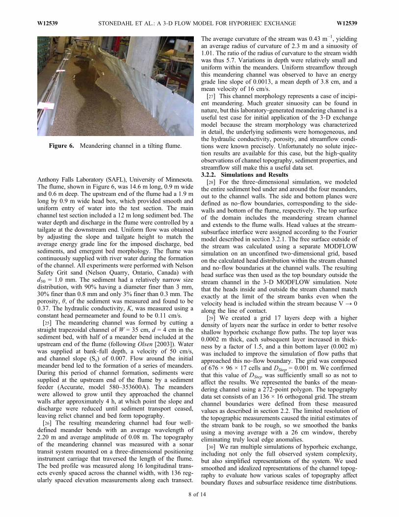
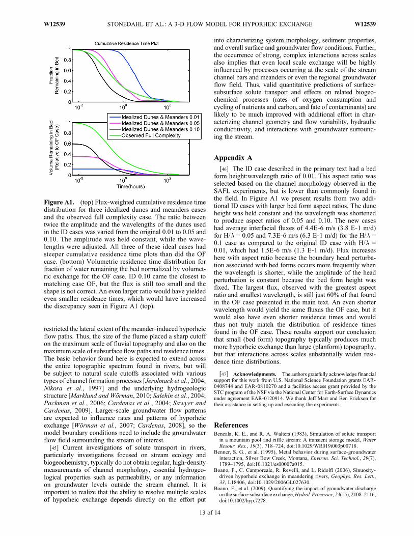
[46] The ID case described in the primary text had a bedform height:wavelength ratio of 0.01. This aspect ratio wasselected based on the channel morphology observed in theSAFL experiments, but is lower than commonly found inthe field. In Figure A1 we present results from two addi-tional ID cases with larger bed form aspect ratios. The duneheight was held constant and the wavelength was shortenedto produce aspect ratios of 0.05 and 0.10. The new caseshad average interfacial fluxes of 4.4E‐6 m/s (3.8 E‐1 m/d)for H/l = 0.05 and 7.3E‐6 m/s (6.3 E‐1 m/d) for the H/l =0.1 case as compared to the original ID case with H/l =0.01, which had 1.5E‐6 m/s (1.3 E‐1 m/d). Flux increaseshere with aspect ratio because the boundary head perturba-tion associated with bed forms occurs more frequently whenthe wavelength is shorter, while the amplitude of the headperturbation is constant because the bed form height wasfixed. The largest flux, observed with the greatest aspectratio and smallest wavelength, is still just 60% of that foundin the OF case presented in the main text. An even shorterwavelength would yield the same fluxas the OF case, but itwould also have even shorter residence times and wouldthus not truly match the distribution of residence timesfound in the OF case. These results support our conclusionthat small (bed form) topography typically produces muchmore hyporheic exchange than large (planform) topography,but that interactions across scales substantially widen resi-dence time distributions.

[47] Acknowledgments. The authors gratefully acknowledge financialsupport for this work from U.S. National Science Foundation grants EAR‐0408744 and EAR‐0810270 and a facilities access grant provided by theSTC program of the NSF via the National Center for Earth‐Surface Dynamicsunder agreement EAR‐0120914. We thank Jeff Marr and Ben Erickson fortheir assistance in setting up and executing the experiments.

ReferencesBencala, K. E., and R. A. Walters (1983), Simulation of solute transport

in a mountain pool‐and‐riffle stream: A transient storage model, WaterResour. Res., 19(3), 718–724, doi:10.1029/WR019i003p00718.

Benner, S. G., et al. (1995), Metal behavior during surface‐groundwaterinteraction, Silver Bow Creek, Montana, Environ. Sci. Technol., 29(7),1789–1795, doi:10.1021/es00007a015.

Boano, F., C. Camporeale, R. Revelli, and L. Ridolfi (2006), Sinuosity‐driven hyporheic exchange in meandering rivers, Geophys. Res. Lett.,33, L18406, doi:10.1029/2006GL027630.

Boano, F., et al. (2009), Quantifying the impact of groundwater dischargeon the surface‐subsurface exchange,Hydrol. Processes, 23(15), 2108–2116,doi:10.1002/hyp.7278.

Figure A1. (top) Flux‐weighted cumulative residence timedistribution for three idealized dunes and meanders casesand the observed full complexity case. The ratio betweentwice the amplitude and the wavelengths of the dunes usedin the ID cases was varied from the original 0.01 to 0.05 and0.10. The amplitude was held constant, while the wave-lengths were adjusted. All three of these ideal cases hadsteeper cumulative residence time plots than did the OFcase. (bottom) Volumetric residence time distribution forfraction of water remaining the bed normalized by volumet-ric exchange for the OF case. ID 0.10 came the closest tomatching case OF, but the flux is still too small and theshape is not correct. An even larger ratio would have yieldedeven smaller residence times, which would have increasedthe discrepancy seen in Figure A1 (top).

STONEDAHL ET AL.: A 3‐D FLOW MODEL FOR HYPORHEIC EXCHANGE W12539W12539

13 of 14

Buffington, J., and D. Tonina (2009), Hyporheic exchange in mountainrivers, part II: Effects of channel morphology on mechanics, scales, andrates of exchange, Geogr. Compass, 3(3), 1038–1062, doi:10.1111/j.1749-8198.2009.00225.x.

Cardenas, M. B. (2008), Surface water‐groundwater interface geomorphol-ogy leads to scaling of residence times, Geophys. Res. Lett., 35, L08402,doi:10.1029/2008GL033753.

Cardenas, M. B. (2009a), Stream‐aquifer interactions and hyporheicexchange in gaining and losing sinuous streams, Water Resour. Res.,45, W06429, doi:10.1029/2008WR007651.

Cardenas, M. B. (2009b), A model for lateral hyporheic flow based onvalley slope and channel sinuosity, Water Resour. Res., 45, W01501,doi:10.1029/2008WR007442.

Cardenas, M. B., and J. L. Wilson (2007), Dunes, turbulent eddies, andinterfacial exchange with permeable sediments, Water Resour. Res.,43, W08412, doi:10.1029/2006WR005787.

Cardenas, M. B., J. L. Wilson, and V. A. Zlotnik (2004), Impact of heteroge-neity, bed forms, and stream curvature on subchannel hyporheic exchange,Water Resour. Res., 40, W08307, doi:10.1029/2004WR003008.

Cardenas, M. B., et al. (2008), Residence time of bedform‐driven hypor-heic exchange, Adv. Water Resour., 31(10), 1382–1386, doi:10.1016/j.advwatres.2008.07.006.

Chaudhry, M. H. (1993), Open Channel Flow, Prentice‐Hall, EnglewoodCliffs, N. J.

Driscoll, T. A. (1996), Algorithm 756: A MATLAB toolbox for Schwarz‐Christoffel mapping, Trans. Math. Software , 22(2), 168–186,doi:10.1145/229473.229475.

Elliott, A. H., and N. H. Brooks (1997a), Transfer of nonsorbing solutes toa streambed with bed forms: Theory,Water Resour. Res., 33(1), 123–136,doi:10.1029/96WR02784.

Elliott, A. H., and N. H. Brooks (1997b), Transfer of nonsorbing solutes toa streambed with bed forms: Laboratory experiments, Water Resour.Res., 33(1), 137–151, doi:10.1029/96WR02783.

Fehlman, H. M. (1985), Resistance components and velocity distributionsof open channel flows over bedforms, M.S. thesis, Colo. State Univ.,Fort Collins, Colo.

Fink, K., and J. Mathews (1999), Numerical Methods Using MATLAB,Prentice‐Hall, Englewood Cliffs, N. J.

Fuller, C. C., and J. W. Harvey (2000), Reactive uptake of trace metals inthe hyporheic zone of a mining‐contaminated stream, Pinal Creek, Arizona,Environ. Sci. Technol., 34(7), 1150–1155, doi:10.1021/es990714d.

Harbaugh, A. W., et al. (2000), MODFLOW‐2000, the US GeologicalSurvey modular ground‐water model: User guide to modularizationconcepts and the ground‐water flow process, U.S. Geol. Surv. Open FileRep., 00–92, 1–121.

Harvey, J. W., and K. E. Bencala (1993), The effect of streambed topogra-phy on surface‐subsurface water exchange in mountain catchments,Water Resour. Res., 29(1), 89–98, doi:10.1029/92WR01960.

Harvey, J. W., and B. J. Wagner (2000), Quantifying hydrologic interac-tions between streams and their subsurface hyporheic zones, in Streamsand Groundwaters, edited by J. B. Jones and P. J. Mulholland, pp. 3–44,doi:10.1016/B978-012389845-6/50002-8, Academic, San Diego, Calif.

Jerolmack, D. J., and D. Mohrig (2005), A unified model for subaqueousbedform dynamics, Water Resour. Res., 41, W12421, doi:10.1029/2005WR004329.

Jerolmack, D. J., et al. (2004), A minimum time for the formation of HoldenNortheast fan, Mars, Geophys. Res. Lett., 31, L21701, doi:10.1029/2004GL021326.

Jones, J. B., and P. J. Mulholland (Eds.) (2000), Streams and Ground-waters, Academic, San Diego, Calif.

Marklund, L., and A. Wörman (2010), The use of spectral analysis‐basedexact solutions to characterize topography‐controlled groundwater flow,Hydrogeol. J., in press.

McKnight, D. M., et al. (2001), Spectrofluorometric characterization ofdissolved organic matter for indication of precursor organic materialand aromaticity, Limnol. Oceanogr., 46(1), 38–48, doi:10.4319/lo.2001.46.1.0038.

Medina, M. A., et al. (2002), Surface water‐ground water interactions andmodeling applications, in Environmental Modeling and Management:Theory, Practice and Future Directions, edited by C. C. Chien et al.,pp. 1–62, DuPont, Wilmington, Del.

Montgomery, D. R., and J. M. Buffington (1997), Channel‐reach morphol-ogy in mountain drainage basins, Geol. Soc. Am. Bull., 109(5), 596–611,doi:10.1130/0016-7606(1997)109<0596:CRMIMD>2.3.CO;2.

Mulholland, P. J., et al. (1997), Evidence that hyporheic zones increase het-erotrophic metabolism and phosphorus uptake in forest streams, Limnol.Oceanogr., 42(3), 443–451, doi:10.4319/lo.1997.42.3.0443.

Nikora, V. I., et al. (1997), Statistical sand wave dynamics in one‐directional water flows, J. Fluid Mech., 351, 17–39, doi:10.1017/S0022112097006708.

O’Connor, B. L., and J. W. Harvey (2008), Scaling hyporheic exchangeand its influence on biogeochemical reactions in aquatic ecosystems,Water Resour. Res., 44, W12423, doi:10.1029/2008WR007160.

Olsen, N. R. B. (2003), Three‐dimensional CFD modeling of self‐formingmeandering channel, J. Hydraul. Eng., 129(5), 366–372, doi:10.1061/(ASCE)0733-9429(2003)129:5(366).

Packman, A. I., and K. E. Bencala (2000), Modeling methods in the studyof surface‐subsurface hydrologic interactions, in Streams and Ground-waters, edited by J. B. Jones and P. J. Mulholland, pp. 45–80,doi:10.1016/B978-012389845-6/50003-X, Academic, San Diego, Calif.

Packman, A. I., and N. H. Brooks (2001), Hyporheic exchange of solutesand colloidswithmoving bed forms,Water Resour. Res., 37(10), 2591–2605,doi:10.1029/2001WR000477.

Packman, A. I., et al. (2006), Development of layered sediment structureand its effects on pore water transport and hyporheic exchange, WaterAir Soil Pollut. Focus, 6(5–6), 433–442, doi:10.1007/s11267-006-9057-y.

Salehin, M., A. I. Packman, and M. Paradis (2004), Hyporheic exchangewith heterogeneous streambeds: Laboratory experiments and modeling,Water Resour. Res., 40, W11504, doi:10.1029/2003WR002567.

Sawyer, A. H., and M. B. Cardenas (2009), Hyporheic flow and residencetime distributions in heterogeneous cross‐bedded sediment, WaterResour. Res., 45, W08406, doi:10.1029/2008WR007632.

Stream Solute Workshop (1990), Concepts and methods for assessingsolute dynamics in stream ecosystems, J. N. Am. Benthol. Soc., 9(2),95–119, doi:10.2307/1467445.

Thibodeaux, L. J., and J. D. Boyle (1987), Bedform‐generated convectivetransport in bottom sediment, Nature, 325(6102), 341–343, doi:10.1038/325341a0.

Tonina, D., and J. Buffington (2009), Hyporheic exchange in mountainrivers, part I: Mechanics and environmental effects, Geogr. Compass,3(3), 1063–1086, doi:10.1111/j.1749-8198.2009.00226.x.

Triska, F. J., et al. (1993), The role of water exchange between a streamchannel and its hyporheic zone in nitrogen cycling at the terrestrial‐aquatic interface, Hydrobiologia, 251(1–3), 167–184, doi:10.1007/BF00007177.

Valett, H. M., et al. (1996), Parent lithology, surface‐groundwaterexchange, and nitrate retention in headwater streams, Limnol. Oceanogr.,41(2), 333–345, doi:10.4319/lo.1996.41.2.0333.

Williams, D. D., and H. B. N. Hynes (1974), The occurrence of benthosdeep in the substratum of a stream, Freshwater Biol., 4(3), 233–256,doi:10.1111/j.1365-2427.1974.tb00094.x.

Winter, T. C., et al. (1998), Ground water and surface water: A singleresource, U.S. Geol. Surv. Circ., 1139, 1–87.

Wörman, A., A. I. Packman, L. Marklund, J. W. Harvey, and S. H. Stone(2006), Exact three‐dimensional spectral solution to surface‐groundwaterinteractions with arbitrary surface topography, Geophys. Res. Lett., 33,L07402, doi:10.1029/2006GL025747.

Wörman, A., A. I. Packman, L. Marklund, J. W. Harvey, and S. H. Stone(2007), Fractal topography and subsurface water flows from fluvial bed-forms to the continental shield, Geophys. Res. Lett., 34, L07402,doi:10.1029/2007GL029426.

Zarrati, A. R., et al. (2005), Mathematical modeling of meanderingchannels with a generalized depth averaged model, J. Hydraul. Eng.,131(6), 467–475, doi:10.1061/(ASCE)0733-9429(2005)131:6(467).

J. W. Harvey, U.S. Geological Survey, 430 National Center, Reston, VA20192, USA. (jwharvey@usgs.gov)A. I. Packman and S. H. Stonedahl, Department of Civil and Environmental

Engineering, Northwestern University, 2145 Sheridan Rd., Evanston, IL60208‐3109, USA. (a‐packman@northwestern.edu; susa@u.northwestern.edu)M. Salehin, Institute of Water and Flood Management, Bangladesh

University of Engineering and Technology, Dhaka 1000, Bangladesh.(mashfiqussalehin@iwfm.buet.ac.bd)A. Wörman, Royal Institute of Technology, Teknikringen 76, SE‐100 44

Stockholm, Sweden. (worman@kth.se)

STONEDAHL ET AL.: A 3‐D FLOW MODEL FOR HYPORHEIC EXCHANGE W12539W12539

14 of 14