A Multiscale Approach to Mesh-based Surface Tension Flows

Nils Thurey Chris Wojtan Markus Gross Greg TurkETH Zurich Georgia Institute of Technology ETH Zurich Georgia Institute of Technology

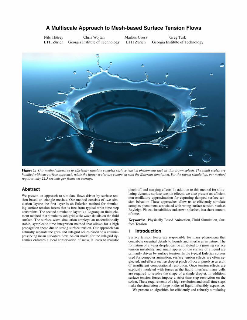
Figure 1: Our method allows us to efficiently simulate complex surface tension phenomena such as this crown splash. The small scales arehandled with our surface approach, while the larger scales are computed with the Eulerian simulation. For the shown simulation, our methodrequires only 22.3 seconds per frame on average.

AbstractWe present an approach to simulate flows driven by surface ten-sion based on triangle meshes. Our method consists of two sim-ulation layers: the first layer is an Eulerian method for simulat-ing surface tension forces that is free from typical strict time stepconstraints. The second simulation layer is a Lagrangian finite ele-ment method that simulates sub-grid scale wave details on the fluidsurface. The surface wave simulation employs an unconditionallystable, symplectic time integration method that allows for a highpropagation speed due to strong surface tension. Our approach cannaturally separate the grid- and sub-grid scales based on a volume-preserving mean curvature flow. As our model for the sub-grid dy-namics enforces a local conservation of mass, it leads to realistic

pinch off and merging effects. In addition to this method for simu-lating dynamic surface tension effects, we also present an efficientnon-oscillatory approximation for capturing damped surface ten-sion behavior. These approaches allow us to efficiently simulatecomplex phenomena associated with strong surface tension, such asRayleigh-Plateau instabilities and crown splashes, in a short amountof time.

Keywords: Physically Based Animation, Fluid Simulation, Sur-face Tension

1 IntroductionSurface tension forces are responsible for many phenomena thatcontribute essential details to liquids and interfaces in nature. Theformation of a water droplet can be attributed to a growing surfacetension instability, and small ripples on the surface of a liquid areprimarily driven by surface tension. In the typical Eulerian solversused for computer animation, surface tension effects are often ne-glected, and effects such as droplet pinch off occur purely as a resultof insufficient computational resolution. Once tension effects areexplicitly modeled with forces at the liquid interface, many cellsare required to resolve the shape of a single droplet. In addition,surface tension forces impose a strict time step restriction on thesolver. These requirements of a high resolution and small time stepsmake the simulation of large bodies of liquid infeasibly expensive.

We present an algorithm for efficiently and robustly simulating

surface tension effects that is based on an a triangle mesh discretiza-tion of the fluid surface. As such, our method is decoupled from theresolution of the computational grid and allows for an efficient sim-ulation of sub-grid scale surface tension effects, including dropletpinch off and surface tension waves. At the same time, it allowsus to separate the small scales of detail that are best simulated onthe surface from the larger scales that are suitable to be resolvedwithin an Eulerian simulation. A key benefit of the surface mesh isthat it allows us to use a robust finite element method to discretizeour model for the surface tension dynamics. Furthermore, as sur-face tension phenomena are driven by the curvature of the surface,we can use the large body of work on discrete surface operators toaccurately calculate curvature and curvature flows of our fluid sur-face. As our method enforces a local conservation of mass, it leadsto realistically bulging surfaces and reproduces natural instabilitiesthat result in pinch off behavior.

The key attributes of our approach to surface tension are as fol-lows:

• A novel method for efficiently simulating sub-grid surfacetension effects that computes wave dynamics on the dis-cretized fluid surface.

• An algorithm that has a significantly relaxed time step restric-tion in comparison to previous approaches in graphics.

• The efficient and robust handling of pinch off, as well as merg-ing effects with local volume preservation on sub-grid scales.

• A simple and efficient non-oscillatory approximation to sub-grid surface tension using mesh-based volume-preservingmean curvature flow

These contributions combine to produce highly detailed anima-tions of surface tension phenomena with subtle secondary effects ata fraction of the cost of previous methods.

We will now briefly outline the different steps of our simulationalgorithm, which are also illustrated in Figure 2. For simulating thefluid, we use a standard solver in combination with a triangle-meshembedded in the Eulerian grid to represent the liquid surface, asdescribed in [Wojtan et al. 2009]. The input to our algorithm is atriangle mesh F representing the liquid interface. First, we advect Fthrough the velocity field given by the previous step in the fluid sim-ulation. Second, we compute a simplified and smoothed version Sof this surface for each connected component of F using a volume-preserving curvature flow with a strength proportional to the spatialand temporal resolution. Next, we calculate the closest points on Sfor all vertices of F , and we use the distance from each vertex to itsclosest point to initialize the height values of the simulated surfacewaves. We solve the wave equation on F using an implicit New-mark scheme with a wave propagation speed given by the surfacetension strength. We then reposition the vertices of F according tothe resulting solution, giving us an updated position of the fluid sur-face. Meanwhile, the curvature of S represents the remainder of thesurface tension forces that can be represented within the Eulerianfluid simulation. We apply a similar framework for animating sur-face tension on the scale of the fluid grid by computing a secondstep of volume-preserving curvature flow on S, yielding a surfaceT . Similar to previous work, the pressure boundary conditions forthe surface tension on the Eulerian grid can be computed using thedistance of a point on S towards its closest point on T . Finally, thesimulation proceeds to solve for a divergence-free velocity field,taking into account the surface tension boundary conditions com-puted as outlined above.

2 Related WorkWhile some of the first fluid simulations in computer graphics wereperformed by Kass and Miller in [1990] as well as [Foster andMetaxas 1996], a large body of work is now based on the simula-tion approach introduced in [Stam 1999; Foster and Fedkiw 2001;

Enright et al. 2002], and many extension of this approach havebeen proposed in the following years. Examples of such exten-sions are coupling with thin shells [Guendelman et al. 2005], im-proved boundary conditions for rigid objects [Batty et al. 2007], amore accurate advection step [Selle et al. 2008], and stable two-waycoupling with deformable objects [Robinson-Mosher et al. 2008].A detailed description can be found, e.g., in the book by Bridson[2008], and we also employ this type of solver in our work. How-ever, while level-sets [Osher and Sethian 1988] are used often torepresent the free surface of a liquid, we use the method of [Wojtanet al. 2009] to track the fluid surface and handle topology changes.This method is based on an accurate Lagrangian surface represen-tation, and produces temporally coherent surfaces, which makes ita good basis for surface tension simulations. In addition, it allowsus to overcome problems typically associated with computing cur-vature driven flows on meshes: the mesh is re-sampled to preventa clustering of vertices, and topological changes are handled by ro-bustly and locally re-constructing the mesh. Apart from this classof solvers, different approaches have been introduced, such as par-ticle based discretizations [Muller et al. 2003], or model reduction[Treuille et al. 2006]. We will focus on the commonly used Eulerianfluid solvers in this work.

Surface tension was recognized as an important aspect of fluids,and the method of Kang et al. [2000] is a popular choice to com-pute the surface tension boundary conditions. The discontinuitiesacross the liquid-air interface for boundary conditions have beenaddressed in [Hong and Kim 2005], while [Muller et al. 2003] dis-cuss surface tension forces for SPH simulations. Because purelyEulerian surface tension simulations do not behave properly at lowgrid resolutions, [Losasso et al. 2004] used an octree data structureto simulate surface tension effects. Contact angles of liquids withsurface tension are discussed by [Wang et al. 2005], while [Wanget al. 2007] use a shallow water solver on obstacle surfaces to com-pute the motion of drops and streams of liquid. We similarly usea surface based wave solver, but use a temporally changing dis-cretization of the liquid surface itself to solve the wave dynamics.We make use of a solver similar to [Angst et al. 2008], where waveswere simulated on animated characters with a fixed connectivity.

Specialized techniques have been proposed for simulating sur-face tension phenomena such as drops and bubbles. Bubbles andfrothing liquids were simulated in [Cleary et al. 2007], [Kim et al.2007] focused on volume control for foam structures, and [Kim andCarlson 2007] presented a fast model for strongly bubbling fluids.[Zheng et al. 2006] introduced a regional level set method witha semi-implicit surface tension scheme for simulating bubbles. Amodel for both drops and bubbles, motivated by the Weber num-ber of the fluid, was proposed by [Mihalef et al. 2009]. While thesemodels handle their respective effects very well, our work focuseson the accurate modelling of the underlying surface tension dynam-ics to recreate phenomena such as droplet pinch off.

One inherent difficulty in direct simulations of surface tensionflows is the strict limitation of the timestep. This topic was ad-dressed in [Cohen and Molemaker 2004], who proposed a methodto perform multiple surface tension driven advection steps persolver iteration. This approach better resolves the surface tensiondynamics in time while safely taking larger time steps in the restof the fluid simulation, but is not closely related to the underly-ing physics because it decouples the surface tension and pressureforces. Recently, Sussman and Ohta [2009] proposed a method torelax the time step restrictions from O(∆x3/2) to O(∆x) by perform-ing a volume preserving mean curvature flow for the computationof the surface tension boundary conditions. While our approach issimilar in nature, we compute surface tension on a mesh instead ofa regular grid, and we perform an additional simulation at sub-gridscales.

Sub-Grid Scale Surface Tension

Grid Scale Surface Tension

Sub-Grid Scale Surface TensionSub-Grid Scale Surface TensionSub-Grid Scale Surface TensionSub-Grid Scale Surface TensionSub-Grid Scale Surface Tension

Grid Scale Surface TensionGrid Scale Surface TensionGrid Scale Surface TensionGrid Scale Surface Tension

FS

Liquid SurfaceVolume-Preserving

Mean Curvature FlowCorresponence

F to SSub-Grid

Surface DynamicsUpdated Position

Volume-Preserving Mean Curvature Flow

CorresponenceS to T

Eulerian Mapping Fluid Simulation

T

F

S

Figure 2: Overview of our surface tension approach. The two rows illustrate the steps performed for the sub-grid surface tension dynamicsin the top row, and the Eulerian surface tension in the bottom row.

As we make use of an explicit surface discretization, we candraw from the many works on shape operators for discrete surfaces.A good overview can be found in [Botsch et al. 2007]. Smoothingoperations on meshes have been widely investigated, e.g., in [Des-brun et al. 1999], where an implicit scheme was presented. We willmake use of volume preserving mean curvature flows on meshes, aswas described in [Eckstein et al. 2007].

3 Fluids with Surface TensionThe dynamics of an incompressible viscous fluid with surface ten-sion can be described by the Navier-Stokes (NS) equations:

ut +(u ·∇)u =− 1ρ

∇p+ν 4u+g+σκ (1)

∇ ·u = 0 . (2)

Here, u is the velocity of the fluid, ut its temporal derivative, ρ thefluid density, g gravity, and σ denotes the surface tension coeffi-cient, which, multiplied with curvature normal of the liquid inter-face κ , gives the surface tension force. Note that the surface tensionterms are only evaluated at the liquid-gas interface. The NS equa-tions are typically discretized on a Eulerian grid with cell size ∆xand a time step of ∆t, using a staggered MAC grid for storing thevelocity information.

For level-set based surface representations, an established wayto implement surface tension effects is to compute κ with the sec-ond derivatives of the signed distance function. The surface tensionforces are included as a pressure jump across the interface, and themethod of [Kang et al. 2000] can be used to include these bound-ary conditions in the fluid solver. This approach gives stable resultsfor a moderate range of surface tension strengths. To improve sta-bility, [Sussman and Ohta 2009] propose a method to compute theσκ term not directly from the level-set, but by first computing avolume-preserving mean curvature flow (VCF) of the liquid inter-face. The distance of the original towards the evolved surface is thenused to compute the pressure boundary conditions. This strategy ef-fectively integrates the forces for the upcoming time step taking intoaccount the surface evolution, and it leads to a significant increasein stability.

However, the methods above still have to fully rely on the Eule-rian grid to resolve features of the interface. As such, several cells

are required to accurately resolve a single drop, and for featuresclose to the size of a cell ∆x the methods become inaccurate andunstable. When directly evaluating the curvature from the level-set,this can lead to noticeable ghost forces, and smaller drops can startto move randomly through the air. Furthermore, the surface tensionmethod based on VCF computes a level set advection to resolve thecurvature flow, and as such, small features can easily disappear, re-sulting in a significant mis-estimation of the surface tension forces.

These problems are closely related to the fact that the size of thelargest stable time step for surface tension flows is strongly gov-erned by the surface tension coefficient σ . Even though the meth-ods outlined above can overcome this restriction, a small time stepis required to accurately resolve the motion of capillary waves. Sur-face waves in a liquid are typically driven by gravity as well assurface tension. Under the assumption that the gas around the liq-uid has a negligible density, the dispersion relation, relating angularfrequency ω to wave number k, simplifies to

ω2 =

(|g|+ σ

ρk2

)|k| . (3)

Note that for large k, which means spatially very small waves,surface tension dominates due to the k2 factor, while large waveswith small k are driven primarily by gravity. The phase velocityvp = ω/k of a water wave is thus given by

√gk for gravity driven

waves, and by |k|3/2ρ/σ for surface tension driven waves. This di-rectly implies that the smallest waves resolved on the grid would re-quire a time step proportional to ∆x3/2. Note that even though semi-Lagrangian methods are unconditionally stable, surface waves donot transport mass, but are represented locally by circular motions,and thus would still require a very small time step to be resolved.

This stringent restrictions caused by surface tension have led toalgorithms that perform multiple computational steps for the sur-face tension during a single step of the fluid simulation. [Hochsteinand Williams 1996] predict the curvature of the surface for the nexttime step, and [Cohen and Molemaker 2004] perform additionaladvection operation to evolve the surface based on surface ten-sion forces. [Sussman and Ohta 2009] can be seen in a similar lineof thought, performing multiple iterations to evolve the volume-preserving curvature flow for calculating the surface tension forces.Our method takes this idea further, by using a wave equation solver

Figure 3: This image shows a liquid surface after a drop impact.A normal simulation is shown on the left, while the right imagedemonstrates the small scales waves our method can resolve at thesurface.

to compute the dynamics of the capillary waves. We use an implicit,symplectic solver for this step, which means that we can handlewaves of arbitrary propagation speed while conserving energy. Inaddition, we use a VCF to compute a base surface for the waveequation solver, which ensures that we simulate waves on the cor-rect scale and re-introduces non-linear behavior into the linearizedwave equation dynamics.

Given a surface tension coefficient σ , we split the overallstrength into two components σ = σs +σg, where σs parametrizesthe surface wave simulation, while the remaining strength σg is in-cluded in the grid-based simulation. Note that we could in theorysplit the forces arbitrarily: for σ = σs all surface tension dynam-ics would be handled with our sub-grid model, while for σ = σg,the full surface tension strength would be calculated on the grid. Inpractice, we will use a geometric separation based on the grid reso-lution, so that the fluid simulation includes as much as it can resolveon the grid, while all smaller surface details are resolved with thewave equation. This is made possible by the fact that the algorithmto compute surface tension using a VCF resembles a surface fairingoperation and effectively smoothes spatial frequencies according tothe strength of the flow.

4 Mean Curvature FlowFirst we will explain how to compute the smoothed version of theoriginal fluid surface that is represented as a triangle mesh. It wasshown by Sussman et al. in [2009] that the surface tension forcesintegrated over the length of a time step can be related to the dis-tance of the liquid surface to another version of the surface advectedby a volume preserving mean curvature flow (VCF). In the limit,the solution of the VCF will converge to one or more spheres withthe same overall volume as the fluid component, which is exactlythe result an isolated surface tension fluid simulation with viscos-ity would give. Note that a single component might be split intopieces by the surface tension, and thus form multiple spheres. Wecompute the smoothed surfaces S and T using a VCF, but solve theVCF directly on a surface mesh instead of a grid. In addition, we usethis method for both layers of our simulation: for the surface ten-sion forces on the grid, and the sub-grid scales on the fluid surface.Thus, in our case, S provides a separation of small spatial scaleswhich will be handled by our surface dynamics model and largerscales for the Eulerian fluid simulation. As a first step we have tosolve for a VCF of the initial and possibly very detailed surface ofthe liquid. Here, we can make use of the large body of research oncurvature flows for meshes. A general mean curvature flow of theset of vertex positions X of a triangle mesh can be formulated as

Xt = γ∇2X , (4)

where γ is the strength of the curvature flow, and the t subscriptdenotes a temporal derivative with respect to the smoothing time.Note that, by construction, Eq. (4) is equivalent to Xt = −2γκn,with κ denoting the mean curvature , and n the surface normal. Thisbasic form evolves the vertices locally according to their Laplacian,

which we discretize with the standard Laplace-Beltrami operatoraccording to [Desbrun et al. 1999]. For a function f that takes thevalue fi at a vertex vi, the discrete Laplace-Beltrami operator canbe formulated as

∇2 f =

12Ai

∑vk∈N (vi)

(cotαk + cotβk)( fk− fi) , (5)

where the area of the barycentric dual cell associated with a vertexvi is denoted by Ai, and the neighborhood of a vertex v is denotedas N (v), consisting of the adjacent vertices vk.

This general form can be turned into a volume preserving surfaceflow by averaging the local deformations around a neighborhood ofeach vertex, as described by Eckstein et al. in [2007]. Similarly, wecompute an averaged curvature κavg for each connected componentof our surface mesh with

κavg =∑vi

Aiκi

∑viAi

, (6)

and evolve the surface with

Xt =−2γ(κ−κavg)n . (7)

This system of equations is solved iteratively for a duration te. Forthe boundary conditions of the Eulerian grid, te is given by te

grid =∆tσg, while for the surface dynamics it is proportional to the gridresolution ∆x, and is computed as te

grid = ∆t(α +∆x). We introducea parameter α here to manually increase the strength of the VCF forthe sub-grid scales. We have found that the Eulerian solver typicallyhas difficulties resolving scales on the size of one to two grid cells,and we make sure these scales are resolved by the surface wavedynamics by choosing α on the order of the grid cell size. This tiesthe geometric differences between the surfaces F and S to the gridsize of the simulation. It is a result of our desire to cleanly separategrid-scale volumetric physics from sub-grid-scale surface physics.

We can speed up this process by simplifying the mesh to matchthe grid resolution in a first step. We do this by computing a signeddistance field from the mesh, and then reconstruct the mesh froma level-set of this distance field using marching cubes. This imme-diately gives us a mesh that closely resembles the details that arerepresentable with the given grid resolution. Note that an alterna-tive would be to continue collapsing all edges that are smaller than∆x, but we have found the results from the level-set reconstructionare temporally more stable and are cheaper to compute. To ensurethat even fine details of the mesh such as thin sheets and small dropsare resolved on the grid, we triangulate the isosurface not at zero butfor a thickened level set of

√3/2 ∆x. We handle each disconnected

component of the mesh separately, to make sure two separate com-ponents do not erroneously merge during the reconstruction fromthe signed distance field. This means, that we can use a strength ofte = ∆tα for the VCF of the wave solver.

Note that, despite the thickened level-set, we can guarantee thatthe surface after the VCF has the same volume as the input sur-face using the volume rescaling technique of Section 8. Our ex-periments have shown that the thickened grid-based re-samplingscheme mentioned above is faster and more consistent than thepurely Lagrangian approach based on edge collapses. The grid-based scheme prohibits topological artifacts due to thin regions, al-though it can cause close regions of a single component to mergetogether. We did not notice any artifacts in practice, so we used thisscheme to generate the examples of Section 10.

Another advantage of simplifying the initial mesh in a first step isthat this typically reduces the number of vertices significantly, andthe complexity for solving Eq. (7) directly depends on the num-ber of vertices. In addition, the mesh S typically has a feature sizeon the comparably large scale of the underlying grid, which makes

Input Mesh Laplacian Smoothing VCF with GlobalAveraging

VCF with LocalAveraging

Figure 4: Here a comparison of the different techniques for curva-ture flow can be seen. The input mesh is shown on the left, Lapla-cian smoothing second from left. Note that the VCF with global av-eraging behaves similarly to Laplacian smoothing, but conservesvolume by pushing the whole surface outward. In contrast to this,local averaging conserves volume by locally bulging the surface.

the curvature flow cheap to compute. This is important, as the stepsize of our explicit curvature flow scheme is proportional to the fea-ture size squared. For highly detailed meshes, the implicit schemedescribed by [Eckstein et al. 2007] can yield a significant speedup. A faster, but less accurate alternative to computing this type ofvolume-preserving curvature flow is to use a global κavg in equationEq. (7) by computing a single volume-weighted average curvaturefor each component. We will use both methods interchangeably inthe following. While Figure 7 and Figure 1 make use of the localcomputation of Eq. (6), the other examples below make use of thefaster per component averaging.

In a next step, we use the mesh S computed with the volume-preserving mean curvature flow to solve for the surface dynamicson the input mesh F . We will describe how to compute correspon-dences between the two meshes in the following. This step will beused to initialize the wave equation in Section 6 and set the bound-ary conditions on the grid in Section 9.

5 Mesh CorrespondenceWe now have the initial, unmodified liquid surface F , and a simpli-fied version S that was evolved in a VCF. As S represents the targetstate towards which F should evolve due to surface tension, we nextmap the vertices of F to their closest points on S.

To do this efficiently, any spatial data structure, such as grids,trees or hash tables is applicable. For our implementation, we havechosen to insert the locations of the vertices xS of S into a kd-treeand query the closest point xS

i to each vertex xi of F using this tree.We then check whether there is an even closer point xS

i to xi onthe triangle fan around xS

i . Note that due to the VCF the surfacemight have shifted, and we have to make sure not to compute theclosest point on the wrong side of thin fluid surfaces. To preventthis, we only return points from the kd-tree query whose normalsalign with the normal of xi. After this step, each vertex xi on Fhas a corresponding point xS

i on S. The set of points xSi on S will

later on represent the reference surface with respect to which wesolve the wave equation. The signed distance hi between the twocorresponding points can be computed with

hi = (xSi −xi) ·nS

i , (8)

where nSi is the normal of the surface S at xS

i . These distances cannow be used to solve for the surface dynamics. Given a new waterheight h′i computed from the wave dynamics, the updated positionsof the vertices is computed with

xi = xSi +h′in

Si . (9)

6 Wave Simulation on the MeshTo efficiently compute the motion of capillary waves on the meshsurface, we linearize the surface tension dynamics with the classicalwave equation. The wave equation is an often-used second order

differential equation in which the normal acceleration of verticalelevations h is related to their second derivatives:

htt = c2∇

2vi

h . (10)

Here htt denotes the second derivative with respect to time. Thevalues of h for each vertex of F are given by Eq. (8), and c2 = σs.

We perform the wave simulation on the triangle mesh F that rep-resents the liquid surface. Similar to [Angst et al. 2008], we use afinite element discretization of the height values. The surface heightis a scalar function that is represented with linear basis functions,and whose values hi are located at the vertices of the triangle mesh.This leads to the commonly used operator with cotangent weightsfor the second derivatives according to Eq. (5).

To overcome the problem of energy dissipation while ensuringrobustness, we make use of the Implicit Newmark time integrationscheme [Newmark 1959] that was proposed in [Angst et al. 2008].In the following, we will denote the vector of the height values forall vertices with h and write the evaluation of the Laplacian of has the multiplication with the matrix L. Now, given a time step ∆t,the Newmark integration step in its unconditionally stable form isgiven by (

I− ∆t2

4c2L

)hn+1 = hn +∆thn

t +∆t2

4hn

tt . (11)

These equations represent a sparse system of linear equations; theunknowns are the positions of the next time step hn+1 that can besolved with a standard iterative solver such as a conjugate gradientmethod.

As the Newmark integrator is a symplectic scheme, this leadsto a conservation of energy when solving the wave equation. Wecan manually introduce viscosity into the wave equation solve bymanually scaling the surface heights by a factor of slightly less thanone relative to the average height of the surface. After solving thewave equation, the surface F is updated using Eq. (9).

7 Non-Oscillatory ApproximationWhile the method for simulating dynamic surface tension proposedin Section 6 produces visually-appealing ripple effects on the sur-face, we can also efficiently simulate damped surface tension ef-fects by neglecting surface wave phenomena entirely. As mentionedpreviously, we can use volume-preserving mean curvature flow toproduce a reference surface S. The capillary waves oscillate aboutthis surface, and they will eventually converge to it after the wavemotion damps out. Therefore, S represents a type of steady-state so-lution to the surface tension dynamics. To efficiently simulate sur-face tension in the absence of small-scale capillary waves, all wehave to do is run volume-preserving mean curvature flow on theoriginal surface F by an amount proportional to the surface tensionat each time step of the simulation. Because this approximation canbe efficiently computed even on high resolution surface meshes, itcan be used to simulate detailed droplet effects (See Figure 7).

8 Mass ConservationA beneficial property of the triangle mesh surface representation isthat we can accurately and efficiently compute its volume, e.g., asdescribed in [Muller 2009]. This is necessary, as the overall con-servation of mass can not be guaranteed despite the accurate ad-vection calculation of the mesh vertices, e.g., with a fourth-orderRunge-Kutta method. In addition, steps such as surface subdivision,topological changes, or the re-initialization from the wave equationsolve can cause violations of the conservation of mass. This is es-pecially crucial for smaller liquid volumes, which could completelydisappear due to these errors. We use a rescaling along the surfacenormals to correct for these errors iteratively. Given a desired vol-ume Vt and a current volume Vc with surface area Ac, we choose

a step size of h = Vt−VcAc

, and iterate the following steps. First thepositions of all surface vertices are updated with xi = hni, whereni is the normal of vertex i. We then recompute Vc, and when therelative error ε = (Vt −Vc)/Vt changes sign from one iteration tothe next, reinitialize the step size with h′ = −h/2. This is repeateduntil converging to the desired accuracy. We have used |ε|< 0.005for the examples below, and usually one or two iterations suffice toreach this accuracy.

Note that similar to the other steps of our algorithm, it is impor-tant to perform the volumetric rescaling separately for each con-nected component of the surface. Components with a negative vol-ume, like bubbles, can be treated in the same way. Using the algo-rithm described in [Wojtan et al. 2009] to handle topology changesof the surface, we only need to identify disconnected componentsand update the target volume Vt for each component when a topol-ogy change was registered. This happens infrequently compared tothe overall number of simulations steps.

9 Eulerian Surface Tension ForcesTo compute surface tension forces for the grid-based fluid simula-tion we can re-use several steps of the framework described abovefor computing the sub-grid scale wave dynamics. As in [Sussmanand Ohta 2009], we compute the term σκ from the distance be-tween two surfaces, one of which is evolved in a VCF correspond-ing to the strength of the surface tension. As the difference betweenthe original surface F and the ground surface for the wave equationS is handled as described in Section 6, we perform another step ofVCF with Eq. (7) on S. For this step, the strength is given by σg,yielding an even smoother surface T .

Now we perform another correspondence computation from Sec-tion 5 to match the position of the vertices xi of S with their closestpoints on T , denoted by xT

i . Note that xi is the actual position ofa vertex, while xT

i can lie anywhere on the surface of T . Next wecompute the surface tension strength for all cells of the grid at theinterface with

σgκ = (xTi −xi) ·ni. (12)

As the points in S will typically not align with the centers of thegrid cells, we again use a kd-tree to retrieve the closest point onS with respect to the cell center. We interpolate the data if a closerpoint is found on an adjacent triangle. For this step, we can estimatethe normal at the cell from the signed distance field of S and onlyquery points from the kd-tree with aligning normals. While var-ious approaches could be used to compute the distance from S toT , we decided to use a kd-tree primarily because of its temporallyconsistency. After using this surface tension value as a boundarycondition for the Eulerian fluid solver, we then proceed to advectthe surface mesh F according to the fluid velocities and handletopological changes with a local re-sampling method. The detailsof this process can be found in [Wojtan et al. 2009]. Next we willdemonstrate the capabilities of our method with several test cases.

10 ResultsThe following simulations and performance measurements wereperformed on a standard PC with 3GHz without multi-threading.First, we compare our method to a surface tension computationperformed by calculating the curvature of a level set surface rep-resentation. Several frames of a simulation of two merging dropswith strong surface tension can be seen in Figure 5, where the toprow was performed with the level-set, and the bottom row withour method. In each simulation, the drops have an initial diame-ter of 9 cells. While both simulations result in a similar behavior,our method is able to capture the waves on the surface of the dropthat are caused by the merge. In addition, our method does pre-serve the volume of the fluid, and does not start to drift. However,

Figure 5: Comparison of a level set based surface tension forces(top row) with our method (bottom row). While both simulationsshow an overall similar behavior of the two merging drops, ourmethod is able to capture a capillary wave travelling around themerged drop with a high speed. In addition, our method is muchbetter at conserving volume.

Figure 6: Example of the self-reinforcing instability of a fluid jetcausing droplet pinch off. The images from left to right show thechange in behavior when increasing the surface tension of the liq-uid (σs = 3e-5 to 0.01). In Table 1, the settings for the second sim-ulation from the left can be seen.

the level-set style simulation took less time to compute. We alsocompared the stability of both methods with this setup: while level-set based simulation quickly becomes unstable with an increase insurface tension, our approach gives violently moving, but reason-able, results even for a 50 times higher surface tension coefficient.Because the time step restriction increases super-linearly for suchexplicit schemes, this difference in stability increases strongly athigher simulation resolutions.

The simulations shown in Figure 6 highlights that our methodis able to very efficiently resolve droplet pinch off for liquid jets.This form of instability is caused by slight perturbations of theinitial cylinder that grow over time. If the diameter of the jet issmall enough, this ultimately leads to a pinch off. This phenomenais known as the Rayleigh-Plateau instability, and has been widelystudied in experiments and simulations, see, e.g., [Bush 2004] fordetails. For our simulation, the jet is resolved with less than 5 gridcells in diameter, and the simulation ran at five frames per second.The images from left to right show how the behavior of the jetsdiffers when increasing surface tension. The left-most image hasa surface tension coefficient close to zero, resulting in barely anydroplet pinch off, while the right-most one shows a simulation withstrong surface tension, causing drops to pinch off right below theinlet.

Figure 7: A fast drop is colliding with a planar obstacle, resulting in a horizontal sheet of liquid. The images show simulations with increasingsurface tension (from top to bottom) at the same instants in time. Stronger surface tension causes the liquid sheet to break up earlier.

An example of a larger fluid simulation with a resolution of 1283

can be seen in Figure 9. Here, a larger drop is falling into a body ofwater, and the resulting back splash causes a single drop to pinch offat its end. In this case, the high fluid simulation resolution is nec-essary to counter the numerical viscosity of the fluid simulation’ssemi-Lagrangian advection scheme.

The non-oscillatory approximation of Section 7 is demonstratedin Figure 7, where no grid based surface tension was active. Thesetup is a well studied experimental one: a liquid drop (or jet) withhigh velocity is hitting a planar or curved obstacle, causing a hor-izontal liquid sheet to develop [Clanet and Villermaux 2002]. Thesheet breaks up at a specific radius inversely proportional to the sur-face tension strength. Our method allows us to re-create the effectthat high surface tension causes an early break up, while low sur-face tension results in a large spreading sheet. For this simulation,we make use of the technique presented in [Wojtan et al. 2010] totrack the very thin liquid sheets.

Finally, a simulation of a crown splash can be seen in Figure 1.This phenomenon develops when a drop hits a shallow volume ofwater, and the evolving circular liquid sheet breaks up at its outerboundary, resulting in regularly spaced droplets. For this simula-tion, we have used a combination of the grid-based surface ten-sion forces and the non-oscillatory approximation. By varying thestrength of the grid-based component, we are able to control theevolution of the liquid sheet, as can be seen in the accompanyingvideo. To our knowledge, we are the first in the graphics and com-putational science field to simulate a full crown splash with dropletpinch off, and our method allows us to efficiently perform a very

detailed simulation with a relatively low grid and surface resolu-tion.

11 DiscussionThe complexity of our algorithm predominantly depends on the res-olution of the surface discretization. For a liquid surface mesh Fwith n nodes, and a smoothed version S with m < n nodes, we ob-serve that the following steps have a complexity of O(n): the signeddistance field computation, the calculation of correspondences fromF to S, and solving the wave equation on F . On the other hand, thefollowing steps have a complexity of O(m): computing the volumepreserving mean curvature flow for S and T , the correspondencesfrom S to T , and the calculations of the boundary conditions forthe grid-based simulation. The magnitude of both n and m predom-inantly depends on the surface area of the liquid interface, insteadof the grid resolution.

The simulation settings and computation times for the shownsimulations can be seen in Table 1. The fastest simulation was theRayleigh-Plateau instability from Figure 6 with 0.2 seconds pertimestep on average, while larger simulations, such as the crownsplash from Figure 1 require up to 22.3 seconds per timestep. Forthe simulations shown, are always able to perform a single timestepper frame of animation. The resolution of the fluid simulationsis typically determined by how many cells the solver requires toachieve a viscosity that is low enough to produce the desired mo-tion. Our surface meshes are typically parametrized relative to thegrid resolution, and the small simulations such as Figure 6 have

Figure 8: These images show a simulation purely with our sub-grid wave equation solver, and without Eulerian surface tension forces. Whilethe right drop is moving towards the large drop, it splits up, and finally merges with the large drop. Throughout the simulation, detailedcapillary waves can be seen on the surfaces of the drops.

Figure 9: A drop is falling into a body of water. The strong surfacetension causes a reinforcement of the instabilities during the backsplash, and finally results in a drop pinching off.

around 2100 vertices for the mesh, while larger ones such as Fig-ure 1 resolve the surface with up to 270 thousand vertices. Similarly,the amount of time that is required for our algorithm is determinedby the complexity of the surface. For larger fluid simulations, suchas Figure 9, on average one third of the overall time is spent forthe surface tension calculations, while others, such as the large sur-faces of Figure 7, require two thirds of the overall time to computethe surface tension dynamics.

Note that we model the non-linear surface tension behavior of afluid simulation with a linear wave equation. We originally imple-mented a fully non-linear wave solution for the sub-grid scale dy-namics, but our early attempts were plagued with self-intersectionsand numerical instabilities. The linearized version avoids theseproblems. However, the linearization also means that we can onlysimulate a single wave propagation speed given by the choice ofthe parameter c in Eq. (10). However, we achieve a non-linear be-havior even without an underlying fluid simulation due to the factthat the positions updated by the wave equation solve are the inputfor the next mesh simplification and smoothing step, as describedin Section 4. In the limit, our wave equation solver will iterativelyconverge towards a uniform height on the smoothed mesh S, whichin turn will converge towards one or more spheres. This means thatour method shows the desired behavior for a flow driven by surfacetension and converges towards spheres as the final shapes for eachdisconnected component. However, some effects that are missingwith only surface waves are the lower frequency oscillations of thesurface, which occur on the scale of the smoothed surface S. In con-trast to the small scale capillary waves, these larger oscillations canby construction be resolved on the Eulerian grid, and we can re-use many components of the algorithm above to compute surfacetension boundary conditions for the grid based fluid simulation.

An important property of the wave equation is its ability to lo-cally preserve the volume of the surface height function. This meansthat it is able to capture, e.g., the effect of a bulging front of a fluidsheet even when the sheet is much smaller than a grid cell. It canthus capture effects such as the breakup of thin sheets and dropletpinch off without having to rely on a Eulerian fluid simulation.

Our approach to surface tension does have some limitations. Thesurface wave equation does not completely conserve the mass of theoverall fluid, but more specifically, that of the represented heights.This fact, in combination with the inaccuracies of the iterative solvemake it necessary to enforce mass conservation with the method ex-plained in Section 8. Luckily, we can accurately measure the initialvolume of each component and keep its mass constant. In addi-tion, despite the energy conserving nature of our implicit solver, theequation can lose energy due to the re-sampling of the underlyingmesh. We currently only linearly interpolate the wave equation vari-ables for triangle subdivisions and edge collapses, so higher-orderinterpolations could help to conserve energy.

In addition, as with any grid based method, our Eulerian ap-proach for surface tension forces can be inaccurate for fluid compo-nents the size of a grid cell, because the boundary conditions can notbe accurately represented on this scale anymore. We can however,reduce the strength of the Eulerian surface tension for connectedcomponents with a volume on the order of a grid cell, because wecan rely on our sub-grid model to handle its dynamics.

12 Conclusion and Future WorkWe have presented a method to simulate surface tension flows us-ing a mesh-based surface representation. Our method handles gridbased surface tension forces with high stability and allows for effi-cient simulations of fast capillary waves on the liquid surface. Thisenables detailed simulations featuring strong surface tension forceswith droplet pinch off as well as capillary waves. In addition, wehave shown how to use a fast approximation of the wave equationsolution with a steady state surface flow to yield highly detailedsurfaces. The mesh surface makes it possible to accurately computevolume preserving mean curvature flow, which is the basis for ourgrid based forces and sub-grid dynamics. Our approach allows usto simulate a wide range of surface tension phenomena with a lowcomputational cost.

There are a number of extensions to our basic technique that weare considering as future work. We would like to include a non-linear wave solver, to more accurately handle dispersive capillarywaves on the liquid surface. In addition, our method could be usedto create interesting effects for bubbles and underwater phenomena,instead of only drops. For the grid based surface tension component,we would like to use more accurate immersed boundary methodsfrom [Peskin 2002]. Finally, it would be intereting to include in-teractions with obstacle surfaces, such as enforcing certain contactangles as in [Wang et al. 2005].

AcknowledgementsThis work was funded by NFS grants CCF-0811485 and CCF-

0625264. We also thank the anonymous reviewers for their helpfulcomments.

grid mesh time σg α σs

Figure 5 753 0.5 1.0s 0.4 0.002 0.015Figure 6 152x75 0.5 0.2s 5e-5 0.001 4e-3Figure 7 1602x80 0.25 12.6s 0 0 1.5e-4∗

Figure 9 1283 0.5 14.1s 2e-4 0.003 2e-4Figure 8 503 0.45 1.0s 0 0.01 2.25e-3Figure 1 1802x50 0.55 22.3s 3e-6 0 3.5e-4∗

Table 1: This table shows the settings used for our simulations.The mesh resolution is given relative to the grid size, while the tim-ing is the average simulation time per frame of animation. σs withan asterisk ∗ denotes simulations with the non-oscillatory approxi-mation.

ReferencesANGST, R., THUREY, N., BOTSCH, M., AND GROSS, M. 2008.

Robust and Efficient Wave Simulations on Deforming Meshes.Computer Graphics Forum 27 (7) (October), 6, 1895 – 1900.

BATTY, C., BERTAILS, F., AND BRIDSON, R. 2007. A fast varia-tional framework for accurate solid-fluid coupling. ACM Trans.Graph. 26, 3, 100:1–100:7.

BOTSCH, M., PAULY, M., KOBBELT, L., ALLIEZ, P., LEVY, B.,BISCHOFF, S., AND ROSSL, C. 2007. In SIGGRAPH ’07: ACMSIGGRAPH 2007 courses, ACM, 1.

BRIDSON, R. 2008. Fluid Simulation for Computer Graphics. AK Peters.

BUSH, J. 2004. MIT Lecture Notes on Surface Tension. Mas-sachusetts Institute of Technology.

CLANET, C., AND VILLERMAUX, E. 2002. Life of a smooth liquidsheet. Journal of Fluid Mechanics 462, 307–340.

CLEARY, P. W., PYO, S. H., PRAKASH, M., AND KOO, B. K.2007. Bubbling and frothing liquids. ACM Trans. Graph. 26, 3,97.

COHEN, J. M., AND MOLEMAKER, M. J. 2004. Practical sim-ulation of surface tension flows. In SIGGRAPH ’04: Sketches,ACM, New York, NY, USA, 70.

DESBRUN, M., MEYER, M., SCHRODER, P., AND BARR, A.1999. Implicit fairing of irregular meshes using diffusion andcurvature flow. Proc. SIGGRAPH, 317–324.

ECKSTEIN, I., PONS, J.-P., TONG, Y., KUO, C.-C. J., AND DES-BRUN, M. 2007. Generalized surface flows for mesh processing.In SGP ’07: Proceedings of the Eurographics symposium on Ge-ometry processing, 183–192.

ENRIGHT, D. P., MARSCHNER, S. R., AND FEDKIW, R. P. 2002.Animation and rendering of complex water surfaces. ACMTrans. Graph. 21, 3, 736–744.

FOSTER, N., AND FEDKIW, R. 2001. Practical animation of liq-uids. In Proceedings of ACM SIGGRAPH 2001, 23–30.

FOSTER, N., AND METAXAS, D. 1996. Realistic animation ofliquids. In Graphics Interface 1996, 204–212.

GUENDELMAN, E., SELLE, A., LOSASSO, F., AND FEDKIW, R.2005. Coupling water and smoke to thin deformable and rigidshells. In SIGGRAPH ’05: ACM SIGGRAPH 2005 Papers, 973–981.

HOCHSTEIN, J. I., AND WILLIAMS, T. L. 1996. An implicitsurface tension model. In AIAA Meeting Papers, vol. 96-0599.

HONG, J.-M., AND KIM, C.-H. 2005. Discontinuous fluids. Proc.of ACM SIGGRAPH ’05 24, 3, 915–920.

KANG, M., FEDKIW, R. P., AND LIU, X.-D. 2000. A boundarycondition capturing method for multiphase incompressible flow.

J. Sci. Comput. 15, 3, 323–360.

KASS, M., AND MILLER, G. 1990. Rapid, stable fluid dynamicsfor computer graphics. In the Proceedings of ACM SIGGRAPH90, 49–57.

KIM, T., AND CARLSON, M. 2007. A simple boiling mod-ule. In SCA ’07: Proceedings of the 2007 ACM SIG-GRAPH/Eurographics symposium on Computer animation, 27–34.

KIM, B., LIU, Y., LLAMAS, I., JIAO, X., AND ROSSIGNAC, J.2007. Simulation of bubbles in foam with the volume controlmethod. ACM Trans. Graph. 26, 3, 98.

LOSASSO, F., GIBOU, F., AND FEDKIW, R. 2004. Simulatingwater and smoke with an octree data structure. In Proceedingsof ACM SIGGRAPH 2004, ACM Press, 457–462.

MIHALEF, V., METAXAS, D., AND SUSSMAN, M. 2009. Simula-tion of two-phase flow with sub-scale droplet and bubble effects.In Proceedings of Eurographics 2009, CGF, vol. 28:2.

MULLER, M., CHARYPAR, D., AND GROSS, M. 2003. Particle-based fluid simulation for interactive applications. Proc. of theACM Siggraph/Eurographics Symposium on Computer Anima-tion, 154–159.

MULLER, M. 2009. Fast and robust tracking of fluid surfaces.Proc. of Symposium on Computer Animation.

NEWMARK, N. M. 1959. A method of computation for structuraldynamics. ASCE J. Eng. Mech. Div. 85, 67–94.

OSHER, S., AND SETHIAN, J. 1988. Fronts propagatingwith curvature-dependent speed: Algorithms based on Hamilton-Jacobi formulations. Journal of Computational Physics 79, 12–49.

PESKIN, C. S. 2002. The immersed boundary method. Acta Nu-merica 11, 1–39.

ROBINSON-MOSHER, A., SHINAR, T., GRETARSSON, J., SU, J.,AND FEDKIW, R. 2008. Two-way coupling of fluids to rigid anddeformable solids and shells. ACM Trans. Graph. 27, 3, 1–9.

SELLE, A., FEDKIW, R., KIM, B., LIU, Y., AND ROSSIGNAC, J.2008. An unconditionally stable maccormack method. J. Sci.Comput. 35, 2-3, 350–371.

STAM, J. 1999. Stable fluids. In the Proceedings of ACM SIG-GRAPH 99, 121–128.

SUSSMAN, M., AND OHTA, M. 2009. A stable and efficientmethod for treating surface tension in incompressible two-phaseflow. J. Sci. Comput. 31, 4, 2447–2471.

TREUILLE, A., LEWIS, A., AND POPOVIC, Z. 2006. Model re-duction for real-time fluids. ACM Transactions on Graphics 25,3 (July), 826–834.

WANG, H., MUCHA, P. J., AND TURK, G. 2005. Water drops onsurfaces. In ACM SIGGRAPH 2005 Papers, ACM, New York,NY, USA, 921–929.

WANG, H., MILLER, G., AND TURK, G. 2007. Solving generalshallow wave equations on surfaces. In Proc. of the ACM Sig-graph/Eurographics Symposium on Computer Animation, 229–238.

WOJTAN, C., THUREY, N., GROSS, M., AND TURK, G. 2009.Deforming meshes that split and merge. In ACM SIGGRAPH2009 papers, ACM, New York, NY, USA, 1–10.

WOJTAN, C., THUREY, N., GROSS, M., AND TURK, G. 2010.Physics-inspired topology changes for thin fluid features. 1–8.

ZHENG, W., YONG, J.-H., AND PAUL, J.-C. 2006. Simulationof bubbles. In Proc. of the ACM Siggraph/Eurographics Sympo-sium on Computer Animation, 325–333.