A Multiplier Approach to Understanding the

Macro Implications of Household Finance ∗

YiLi Chien

Purdue University

Harold Cole

University of Pennsylvania

Hanno Lustig

UCLA and NBER

January 29, 2008

Abstract

Our paper examines the impact of heterogeneous trading technologies for households on

asset prices and the distribution of wealth. We distinguish between passive traders who

hold fixed portfolios of stocks and bonds, and active traders who adjust their portfolios to

changes in the investment opportunity set. The fraction of total wealth held by active traders

is critical for asset prices, because only these traders respond to variation in state prices

and hence absorb the residual aggregate risk created by non-participants. We calibrate this

heterogeneity to match the equity premium and the risk-free rate. The calibrated model

reproduces the skewness and kurtosis of the wealth distribution in the data. To solve the

model, we develop a new method that relies on an optimal consumption sharing rule and an

aggregation result for state prices. This result allows us to solve for equilibrium prices and

allocations without having to search for market-clearing prices in each asset market separately.

Keywords: Asset Pricing, Household Finance, Risk Sharing, Limited Participation (JEL

code G12)

1 Introduction

There is a growing body of empirical evidence that households behave as if they had access to

different investment opportunity sets, both in terms of the securities they invest in and the extent

to which they actively trade these securities.1 A majority of households does not invest directly

∗

1Campbell (2006) refers to the body of literature that documents this heterogeneity as “household finance”.See Campbell (2006)’s AFA presidential address for a comprehensive discussion of these and other issues relatedto household finance. Initially, this literature gathered evidence mostly from brokerage accounts, starting withSchlarbaum, Lease, and Lewellen (1978), Odean (1998) and Odean (1999), and from the Survey of ConsumerFinances. More recently, a comprehensive dataset of Swedish households has been studied by Massa and Simonov(2006), Calvet, Campbell, and Sodini (2007a) and Calvet, Campbell, and Sodini (2007b).

in equity, in spite of the sizeable historical equity premium. Even among those who participate

in equity markets, Calvet, Campbell, and Sodini (2007a) find that sophisticated investors invest a

larger share of their wealth in equity and realize higher returns, while less sophisticated investors

take a more cautious approach. In addition, there is evidence that the portfolios of less sophisticated

investors display more inertia (Calvet, Campbell, and Sodini (2007b)). Campbell (2006) infers that

some households voluntarily limit the set of assets they decide to trade for fear of making mistakes,

at the cost of forgoing higher returns.

These empirical findings lead us to introduce heterogeneous trading technologies in an otherwise

standard model. A version of our model that calibrates this heterogeneity to match the equity

premium and the risk-free rate, also matches the skewness and kurtosis of the wealth distribution in

the data, and it replicates the relation between wealth and equity holdings in the data. Our model

identifies heterogeneity in financial sophistication as an important driver of wealth inequality. To

solve this model, we develop a new method that does not rely on a price adjustment algorithm to

clear each asset market separately.

We introduce heterogeneity in trading technologies into an endowment economy with a large

number of agents who are subject to both aggregate and idiosyncratic shocks, and who have

constant relative risk aversion (CRRA) preferences with coefficient α. Our model distinguishes be-

tween passive traders, who trade fixed-weighted portfolios of bonds and equities, and active traders,

who optimally re-adjust their portfolio holdings over time. We capture the differences in trading

technologies by imposing different measurability restrictions on the household’s time-zero trading

problem. These restrictions govern how net wealth is allowed to vary across different states of the

world. We use the multipliers on these constraints to derive a consumption sharing rule for house-

holds and an analytical expression for the stochastic discount factor. Importantly, the household’s

consumption sharing rule does not depend on the trading technology, only the dynamics of the

multipliers do. The equilibrium stochastic discount factor only depends on aggregate consumption

growth and a weighted average of these multipliers –the −1/α-th moment. We refer to this simply

as the aggregate multiplier.

In our approach, this household multiplier is a new state variable that replaces wealth. We

characterize its dynamics by means of a simple updating rule. This rule depends on the trading

technology of the household. The individual’s multiplier updating rule and the implied updating

rule for the aggregate multipliers completely characterize equilibrium allocations and prices.

We apply our method in a calibrated version of the model. The heterogeneity in trading

technologies is calibrated to match the equity risk premium and the risk-free rate for a risk aversion

coefficient of five. Introducing heterogeneity in trading technologies considerably improves the

asset pricing predictions of the model, without imputing excessive cyclical variation to the wealth

distribution. In addition, this heterogeneity in financial sophistication can almost entirely account

2

for the skewness and kurtosis of the wealth distribution and for the relation between equity holdings

and wealth in the data.

In our model, all the passive traders under-invest in stocks. To capture the richness of observed

trading behavior in the data, we distinguish between passive traders who hold no stocks, the

non-participants, and diversified passive traders who trade the market portfolio, i.e. a claim to

aggregate consumption. At the aggregate level, the non-participants create residual aggregate

risk that ends up being absorbed only by the active traders, not by the passive equity investors or

diversified traders. The non-participants create residual aggregate risk, because they consume “too

much” in low aggregate consumption growth states (recessions) and “too little” in high aggregate

consumption growth states (expansions). On the other hand, the active traders concentrate their

consumption in “cheap” aggregate states (states with low state prices for aggregate consumption).

Hence, to clear the goods market, the equilibrium state prices have to be much higher in recessions

to induce a small segment of active traders to consume less, and much lower in expansions to

induce them to consume more.

The interaction between a small segment of active traders and a larger segment of passive

traders improves the model’s match with asset prices in the data along two dimensions. First,

due to this interaction, equilibrium state prices are highly volatile and counter-cyclical, but their

conditional expectation –and hence the risk-free rate– is not. Instead, the equilibrium state prices

are highly volatile across aggregate states. The spread in state prices induces the small segment

of active traders to adjust their consumption growth in different aggregate states by enough to

clear the market. Second, the share of total wealth owned by the active traders declines in low

aggregate consumption growth states, because they take highly leveraged equity positions. Hence,

the conditional volatility of state prices increases after each recession since a larger adjustment in

state prices is needed to induce the smaller mass of active traders to clear the goods markets. As a

result, the model endogenously generates counter-cyclical Sharpe ratios, even though the aggregate

consumption growth shocks are i.i.d. Interestingly, as we increase the equity share in the passive

trader portfolios, the volatility of returns increases.

In our model, the consumption of passive traders is more exposed to idiosyncratic risk, because

they fail to accumulate enough wealth to self-insure, while the consumption of active traders is more

exposed to aggregate risk. This heterogeneity in the responsiveness of consumption to aggregate

shocks in the model is consistent with recent evidence by Malloy, Moskowitz, and Vissing-Jorgensen

(2007), who find that wealthier stockholders have consumption that is much more exposed to

aggregate shocks. The active traders in our model realize much higher returns, as documented

by Calvet, Campbell, and Sodini (2007a), and they adopt a sophisticated trading strategy that

exploits the time variation in the risk premium to do so. In addition, those active traders who

cannot directly insure against idiosyncratic risk have a strong precautionary motive to accumulate

3

wealth. In the calibrated model, they accumulate on average three times more wealth than the

average household in our model, because of their superior trading technology. This mechanism

allows our model to match the skewness and kurtosis of the wealth distribution in the data. Since

these active traders are wealthy on average and since they have a high fraction of equities in their

portfolio, the calibrated model delivers a closer match between wealth and equity shares in the

data.

The method we develop draws heavily on the prior literature. In continuous-time finance, the

martingale approach, which considers the household’s optimization problem in which all trading

occurs at time zero, has been applied to incomplete market environments. In particular, Cuoco and

He (2001) and Basak and Cuoco (1998a) also rely on stochastic weighting schemes to characterize

allocations and prices. Our approach differs because it provides a tractable and computationally

efficient algorithm for computing equilibria in environments with a large number of agents subject

to idiosyncratic risk, as well as aggregate risk, and heterogeneity in trading opportunities. Our

use of measurability constraints to capture portfolio restrictions is similar to that in Aiyagari,

Marcet, Sargent, and Seppala (2002) and Lustig, Sleet, and Yeltekin (2006), while the aggregation

result extends that in Lustig (2006) to an incomplete markets environment. The use of cumulative

multipliers in solving equilibrium models was pioneered by Kehoe and Perri (2002), building on

earlier work by Marcet and Marimon (1999).

Our paper is closely related to Krusell and Smith (1997) and (1998). Krusell and Smith (1998)

consider a production economy with a large number of agents in which individual labor supply

is subject to exogenous idiosyncratic shocks, while the aggregate production function is subject

to aggregate productivity shocks. Households in this economy only trade claims to the physical

capital stock. In this model with a single asset, KS only need to solve a forecasting problem for the

return on capital. This is similar to our computational approach: we solve a forecasting problem

for the growth rate of this aggregate multiplier. However, as soon as they add one additional asset (

e.g. a risk-free bond in Krusell and Smith (1997)), KS need to solve for the market-clearing pricing

function for this asset. Storesletten, Telmer, and Yaron (2003) implement this procedure in an

OLG model with trading in capital and risk-free bonds. Applying this method in our model would

require searching for a new pricing function for each additional aggregate state in each iteration.

Searching for market-clearing prices is hard because, in general, we do not know the mapping from

the wealth distribution to state prices.

Our aggregation result implies that we only need to forecast a single moment of the multiplier

distribution, regardless of the number and the nature of the different trading technologies. We can

directly compute the pricing kernel as a function of this moment. Hence, there is no need to search

for the vector of state prices that clears the various asset markets. To get the forecast exactly right

requires either the entire history of aggregate shocks or the entire multiplier distribution. We show

4

that a truncated history of aggregate shocks delivers very precise forecasts. Finally, solving for the

multiplier updating rule turns out to be simpler and faster than solving the household’s Bellman

equation or consumption Euler equation.

Our quantitative exercise is related to a growing literature on the asset pricing impact of limited

stock market participation, starting with Saito (1996) and Basak and Cuoco (1998b). Our paper is

the first to our knowledge to document the importance of distinguishing between active and passive

traders for understanding asset prices and the wealth distribution. Other papers have focussed

mostly on heterogeneity in preferences (e.g. see Krusell and Smith (1998) for heterogeneity in the

rate of time preference and Vissing-Jorgensen (2002), Guvenen (2003) and Gomes and Michaelides

(2007) for heterogeneity in the willingness of households to substitute intertemporally) and the

heterogeneity in participation decisions (e.g. see Guvenen (2003) and Vissing-Jorgensen (2002)),

rather than trading opportunities2.

There is an active debate about the effects of limited participation on asset prices. Guvenen

(2003) argues that limited participation goes a long way towards explaining the equity premium

in a model with a bond-only investor and a stockholder.3 We put Guvenen’s mechanism to work

in a richer model with idiosyncratic risk, and with heterogeneity in trading technologies among

market participants. Our model endogenously generates counter-cyclical variation in conditional

Sharpe ratios: because the active traders experience a negative wealth shock in recessions, the

conditional volatility of state prices needs to increase in order to get them to clear the market.

However, we show that the cyclicality of the wealth distribution implied by our model is not at

odds with the data. In more recent work, Gomes and Michaelides (2007) also consider a model

with bond-and stockholders, but they add idiosyncratic risk. Their production economy produces

a large risk premium, which they attribute to imperfect risk sharing among stockholders, not to

the exclusion of households from equity markets. In our endowment economy, we show analytically

that market segmentation only affects the risk-free rate, but not risk premia, as long as there is no

predictability in aggregate consumption growth and all traders can trade the market –a claim to

all diversifiable income.

We do not model the participation decision, but we show that the costs of non-participation are

too large in a model with volatile state prices to be simply explained by standard cost arguments.

Instead, one might have to appeal to differences in cognitive ability. In the data, education is a

strong predictor of equity ownership (see Table I in Campbell (2006)). In our model, this seems

plausible given the complexity of the trading strategies that fully realize the welfare gains of asset

2In recent work, Garleanu and Panageas (2007) explore the effects of heterogeneity in an OLG model, whileChan and Kogan (2002) explore the effects of heterogeneity in risk aversion in a habit model

3In his model, investors do not face idiosyncratic risk and hence the risk-free rate is too high in a growingeconomy. The model can match risk premia, but this comes at the cost of too much volatility in the risk-freerate. In related work, Danthine and Donaldson (2002) consider an economy in which workers do not have access tofinancial markets but are insured by firms.

5

market participation.

This paper is organized as follows. Section 2 describes the environment, the preferences and

trading technologies for all households. Section 3 characterizes the equilibrium allocations and

prices using cumulative multipliers that record all the binding measurability and solvency con-

straints. Section 4 describes a recursive version of this problem that we can actually solve. This

section also describes conditions under which market segmentation does not affect the risk pre-

mium. Finally, in section 5 we study a calibrated version of our economy. All the proofs are in

the appendix. A separate appendix with auxiliary results is available from the authors’ web sites.4

We have also made the matlab code available on-line.

2 Model

In this section we describe the environment, and we describe the household problem for each of

different asset trading technologies. We also define an equilibrium for this economy.

2.1 Environment

This is an endowment economy with a unit measure of households who are subject to both aggre-

gate and idiosyncratic income shocks. Households are ex ante identical, except for the access to

trading technologies. Ex post, the households differ in terms of their idiosyncratic income shock

realizations. Some of the households will be able to trade a complete set of securities, but others

will trade a more limited set of securities. All of the households face the same stochastic process

for idiosyncratic income shocks, and all households start with the same present value of tradeable

wealth.

In the model time is discrete, infinite, and indexed by t = 0, 1, 2, ... The first period, t = 0, is a

planning period in which financial contracting takes place. We use zt ∈ Z to denote the aggregate

shock in period t and ηt ∈ N to denote the idiosyncratic shock in period t. zt denotes the history

of aggregate shocks, and, similarly, ηt, denotes the history of idiosyncratic shocks for a household.

The idiosyncratic events η are i.i.d. across households. We use π(zt, ηt) to denote the unconditional

probability of state (zt, ηt) being realized. The events are first-order Markov, and we assume that

π(zt+1, ηt+1|zt, ηt) = π(zt+1|zt)π(ηt+1|zt+1, ηt).

Since we can appeal to a law of large number, π(zt, ηt)/π(zt) also denotes the fraction of agents in

state zt that have drawn a history ηt. We use π(ηt|zt) to denote that fraction. We introduce some

additional notation: zt+1 ≻ zt or yt+1 ≻ yt means that the left hand side node is a successor node

4http://www.econ.ucla.edu/people/faculty/Lustig.html

6

to the right hand side node. We denote by {zτ ≻ zt} the set of successor aggregate histories for zt

including those many periods in the future; ditto for {ητ ≻ ηt}. When we use �, we include the

current nodes zt or ηt in the summation.

There is a single final good in each period, and the amount of it is given by Y (zt), which evolves

according to

Y (zt) = exp{zt}Y (zt−1), (2.1)

with Y (z1) = exp{z1}. This endowment good comes in two forms. The first form is diversifiable

income, which is not subject to the idiosyncratic shock, and is given by (1 − γ)Y (zt). The other

form is non-diversifiable income which is subject to idiosyncratic risk and is given by γY (zt)ηt;

hence γ is the share of income that is non-diversifiable.

All households are infinitely lived and rank stochastic consumption streams {c(zt, ηt)} according

to the following criterion

U(c) = E

{∞∑

t≥1

βtπ(zt, ηt)c(zt, ηt)1−α

1 − α

}, (2.2)

where α > 0 denotes the coefficient of relative risk aversion, and c(zt, ηt) denotes the household’s

consumption in state (zt, ηt).

2.2 Asset Trading Technologies

All of the households have access to only one of four asset trading technologies. We assume

households cannot switch between technologies. It is straightforward to extend the methodology

we develop to allow for exogenous transitions between trading technologies. The probability of

these transitions could even be contingent on the household’s realized shocks.

Households trade assets in securities markets and they trade the final good in spot markets

that re-open in every period. A fraction µ1 of households can trade claims that are contingent on

both their aggregate and their idiosyncratic state (zt, ηt), a fraction µ2 can trade claims contingent

on the aggregate state zt, a fraction µ3 can only trade claims to a share of diversifiable income,

and a fraction µ4 can only trade non-contingent contracts to deliver units of the final good in

the next time the spot market reopens. Later, we show how to include passive traders with any

fixed-weighted portfolio of bonds and stocks.

We refer to the first set of households as the complete traders since they are able to trade a

complete set of Arrow securities. We refer to the second set as the z-complete traders since they

can only offset aggregate risk but not idiosyncratic risk through their asset trading. We think of

them as having access to a menu of stocks and bonds that is rich enough to span the aggregate

7

shocks.5 We refer to the third set of households as the diversified investors since they are trading

a claim to total financial wealth or equivalently a claim to all diversifiable income. We will refer

to the fourth set of households as non-participants, since they only have a savings account. All

traders face exogenous debt constraints.

Since the return on the diversifiable income claim is measurable with respect to the asset trading

structures of the complete and z-complete traders, we assume w.l.o.g. that the households in the

first two partitions can also trade the claim to diversifiable income.

(zt) denotes the price of a claim to diversifiable income in aggregate state zt. In each node,

total diversifiable income is given by (1 − γ)Y (zt). We use q [(zt+1, ηt+1) , (zt, ηt)] to denote the

price of a unit claim to the final good in state (zt+1, ηt+1) acquired in state (zt, ηt). The absence

of arbitrage implies that there exist aggregate state prices q(zt+1, zt) such that

q[(zt+1, ηt+1

),(zt, ηt

)]= π(ηt+1|zt+1, ηt)q(zt+1, z

t),

where q(zt+1, zt) denotes the price of a unit of the final good in aggregate state zt+1 given that we

are in aggregate history zt. From these, we can back out the present-value state prices recursively

as follows:

π(zt, ηt)P (zt, ηt) = q(zt, zt−1)q(zt−1, z

t−2) · · · q(z1, z0)q(z0).

We use P (zt, ηt) to denote the Arrow-Debreu prices P (zt)π(zt, ηt). Let m(zt+1|zt) = P (zt+1)/P (zt)

denote the stochastic discount factor that prices any random payoffs. We assume there is always a

non-zero measure of z-complete or complete traders to guarantee the uniqueness of the stochastic

discount factor.

All households are endowed with a claim to their per capita share of both diversifiable and

non-diversifiable income. Households cannot directly trade their claim to non-diversifiable risk,

though households can hedge this risk to the extent that they can trade a sufficiently rich menu

of securities. For example, the complete households can hedge both their idiosyncratic and their

aggregate risk. We assume that the non-participants cannot hold the claim to equity. During the

initial trading period, they sell their claim to diversifiable income in exchange for non-contingent

discount bonds since claim implicity includes a claim to equity.

Finally, the households face exogenous limits on their net asset positions. The value of the

household’s net assets must always be greater than −ψ times the value of their non-diversifiable

income, where ψ ∈ (0, 1). We allow households to trade away or borrow up to 100% of the value

of their claims to diversifiable capital.

5In our quantitative analysis, since we have only two aggregate states, z-complete traders are in effect activelytrading the stock and the bond.

8

Complete Traders We start with the household in the first asset partition who can trade both

a complete set of contingent bonds as well as claims to diversifiable income. The budget constraint

for this trader in the spot market in state (zt, ηt) as

γY (zt)ηt + at−1(zt, ηt) + σ(zt−1, ηt−1)

[(1 − γ)Y (zt) +(zt)

]− c(zt, ηt)

≥∑

zt+1≻zt

q(zt+1, zt)

∑

ηt+1≻ηt

a(zt+1, ηt+1)π(ηt+1|zt+1, ηt) + σ(zt, ηt)(zt) ∀(zt, ηt), (2.3)

where at−1(zt, ηt) denotes the number of unit claims to the final good purchased at t − 1 for

state (zt, ηt), σ(zt−1, ηt−1) denotes the number of claims on diversifiable income acquired in state

(zt−1, ηt−1), where (zt, ηt) ≻ (zt−1, ηt−1). The period 0 spot budget constraint is given by

(z0) [1 − σ(z0, η0)] ≥∑

z1

q(z1, z0)

∑

η1

a0(z1, η1)π(ηt+1|zt+1, ηt), (2.4)

where z0 and η0 are degenerate states representing the initial position in the planning state at time

0 before any of the shocks have been realized, and where (z0) denotes the price of capital in the

planning stage and q(z1, z0) denotes the price in this stage of a claim to consumption in period 1.

In addition to their spot budget constraint, these traders also face a lower bound on the value of

their net asset position. Let M(ηt, zt) be defined as

M(ηt, zt) = −ψ∑

τ≥t

∑

{zτ�zt,ητ�ηt}

γY (zτ )ητπ(zτ , ητ )P (zτ , ητ )

π(zt, ηt)P (zt, ηt)(2.5)

The lower bound is given by:

at(zt+1, ηt+1) + σ(zt, ηt)

[d(zt+1) +(zt+1)

]≥M(ηt+1, zt+1). (2.6)

The complete trader’s problem is to choose {c(zt, ηt), at(zt+1, ηt+1), σ(zt, ηt)}, a0(z

1, η1) and σ(z0, η0)

so as to maximize (2.2) subject (2.3-2.6).

z-complete Traders The households in the second asset partition have a budget constraint in

the spot market in state (zt, ηt) given by

γY (zt)ηt + at−1(zt, ηt−1) + σ(zt−1, ηt−1)

[(1 − γ)Y (zt) +(zt)

]− c(zt, ηt)

≥∑

zt+1≻zt

q(zt+1, zt)at(z

t+1, ηt) + σ(zt, ηt)(zt) ∀(zt, ηt), (2.7)

where at(zt+1, ηt) denotes the number of claims acquired in period t that payoff one unit if the

aggregate state tomorrow is zt+1, and where ηt ≻ ηt−1. The period 0 spot budget constraint is

9

given by

(z0) [1 − σ(z0, η0)] ≥∑

z1

q(z1, z0)a0(z

1, η0). (2.8)

The z-complete traders face bounds on their net asset position which is given by:

at(zt+1, ηt) + σ(zt, ηt)

[d(zt+1) +(zt+1)

]≥M(ηt+1, zt+1) (2.9)

for each (zt+1, ηt+1) ≻ (zt, ηt). Note here that for each aggregate state tomorrow, zt+1, the mag-

nitude of the bound is determined by the idiosyncratic state ηt+1 in which the present value of

non-diversifiable income is smallest.

The z-complete trader’s problem is to choose {c(zt, ηt), a(zt+1, ηt), σ(zt, ηt)}, a(z1, η0) and

σ(z0, η0) so as to maximize (2.2) subject (2.7-2.9).

Diversified investors We think of diversified investors as trading a claim to all of the di-

versifiable income. The diversified traders effectively hold a fixed portfolio of equity and bonds.

Following Abel (1999), we define equity as a leveraged claim to consumption. Let φ denote the

leverage parameter, let bt(zt) denote the supply of one-period risk-free bonds, and let Rf

t denote

the risk-free rate. We can decompose the aggregate payout that flows from the diversifiable in-

come claim (1 − γ)Y (zt) into a dividend component dt(zt) from equity and a bond component

Rft (z

t−1)b(zt−1) − b(zt). The bond supply adjusts in each node zt to ensure that the bond/equity

ratio equals φ:

b(zt) = φ[(zt) − b(zt)

]

for all zt. The diversified trader invests a fraction φ/(1 + φ) in bonds and the remainder in equity.

This is a natural benchmark, because we show this portfolio is the optimal one (and it is constant)

in the case without non-participants.

These households in the third asset partition have a budget constraint in the spot market in

state (zt, ηt) given by

γY (zt)ηt + σ(zt−1, ηt−1)[(1 − γ)Y (zt) +(zt)

]− c(zt, ηt) ≥ σ(zt, ηt)(zt) ∀(zt, ηt), (2.10)

a degenerate period 0 constraint

(z0) [1 − σ(z0, η0)] ≥ 0, (2.11)

10

and a net asset position bound

σ(zt, ηt)[(1 − γ)Y (zt+1) +(zt+1)

]≥M(ηt+1, zt+1), (2.12)

for each (zt+1, ηt+1) ≻ (zt, ηt). The diversified trader’s problem is to choose {c(zt, ηt), σ(zt, ηt)} and

σ(z0, η0) so as to maximize (2.2) subject (2.10-2.12).

Non-participants The households in the fourth and final partition have a spot budget constraint

in state (zt, ηt) given by

γY (zt)ηt + at−1(zt−1, ηt−1) − c(zt, ηt) ≥

∑

zt+1≻zt

q(zt+1, zt)at(z

t, ηt), (2.13)

where zt ≻ zt−1 and ηt ≻ ηt−1, for states other than the first, and a first period budget constraint

given by

(z0) ≥ a0(z0, η0)

∑

z1

q(z1, z0)π(η1|z1, η0), (2.14)

because they cannot hold the claim to diversified wealth. The asset bound for non-participants is

given by

at(zt, ηt) ≥M(ηt+1, zt+1) (2.15)

for each (zt+1, ηt+1) ≻ (zt, ηt).The non-participant’s problem is to choose {c(zt, ηt), at(zt, ηt)} and

a0(z0, η0) so as to maximize (2.2) subject to (2.13-2.15).

2.3 Equilibrium

For the sake of clarity, we use (e.g.) ηt−1(ηt) to denote the history from zero to t − 1 contained

in ηt. We use the same convention for the aggregate histories. Using this notation, the market

clearing condition in the bond market is given by:

∑

ηt

[µ1a

ct−1(z

t, ηt) + µ2azt−1(z

t, ηt−1(ηt)) + µ4anpt−1(z

t−1(zt), ηt−1(ηt))]π(ηt|zt) = 0,

where ac, az, adiv, and anp denote the bond holdings of the complete-markets, z-complete, equity-

only, and bonds-only traders respectively. The market clearing condition in the output claim

market is given by

∑

ηt

[µ1σ

c(zt, ηt) + µ2σz(zt, ηt) + µ3σ

div(zt, ηt)]π(ηt|zt) = 1.

An equilibrium for this economy is defined in the standard way. It consists of a list of bond and

11

output claim holdings, a consumption allocation and a list of bond and tradeable output claim

prices such that: (i) given these prices, a trader’s asset and consumption choices maximizer her

expected utility subject to the budget constraints, the solvency constraints and the measurability

constraints, and (ii) the asset markets clear.

The next section analytically characterizes the household consumption function and the equi-

librium pricing kernel in terms of the distribution of the household’s stochastic multipliers.

3 Solving for Equilibrium Allocations and Prices

This section reformulates the household’s problem in terms of a present-value budget constraint,

and sequences of measurability constraints and solvency constraints. These measurability con-

straints capture the restrictions imposed by the different trading technologies of households. We

show how to use the cumulative multipliers on these constraints as stochastic weights that fully

characterize equilibrium allocations and prices. Cuoco and He (2001) were the first to use a similar

stochastic weighting scheme in a discrete-time setup.

3.1 Measurability Conditions

We begin by recursively substituting into the spot budget constraints, in order to derive an ex-

pression in terms of future consumption sequences and the initial asset position in state (zt, ηt).

Complete Traders For example, start from the complete traders constraint (2.3), and assume

it holds with equality. Then we can substitute for future a(zt+i, ηt+i), while using the equity

no-arbitrage condition

(zt) =∑

zt+1

[d(zt+1) +(zt+1)

]q(zt+1, z

t),

to obtain the following budget constraint in terms of present value prices:

at−1(zt, ηt)+σ(zt−1, ηt−1)

[(1 − γ)Y (zt) +(zt)

]=

∑

{zτ�zt,ητ�ηt}

[c(zτ , ητ ) − γY (zτ )ητ ]π(zτ , ητ )P (zτ , ητ )

π(zt, ηt)P (zt, ηt).

Rather than carry around both a and σ, we will find it convenient to define net wealth as

at−1(zt, ηt) ≡ at−1(z

t, ηt) + σ(zt−1, ηt−1)[(1 − γ)Y (zt) +(zt)

].

The borrowing constraint in terms of a is given by

at−1(zt, ηt) ≥M(ηt, zt). (3.1)

12

Requiring that condition (3.1) hold for each (zt, ηt) is equivalent to imposing the spot budget

constraints (2.3) and borrowing constraints (2.6) for the complete traders for all t ≥ 1. In addition

we have the period 0 budget constraint:

(z0) =∑

t>0

∑

(zt,ηt)

[c(zt, ηt) − γY (zt)ηt

]π(zt, ηt)P (zt, ηt). (3.2)

It is straightforward to show that the spot budget and debt bound constraints for the other types

of traders imply that condition (3.1) hold for each (zt, ηt) and that condition (3.2) holds.

However, the limits on the menu of traded assets also imply additional measurability constraints

which reflect the extent to which their net asset position can vary with the realized state (zt, ηt).

z-complete Traders The z-complete traders face the additional constraint that at−1(zt, ηt) is

measurable with respect to (zt, ηt−1). Since the payoff of the stock σ(zt−1, ηt−1) [(1 − γ)Y (zt) +(zt)]

is measurable with respect to(zt, ηt−1), requiring that at−1(zt, ηt) = at−1(z

t, ηt) for all zt, and ηt, ηt

such that ηt−1(ηt) = ηt−1(ηt) is equivalent to requiring that

at−1(zt,

[ηt−1, ηt

]) = at−1(z

t,[ηt−1, ηt

]), (3.3)

for all zt, ηt−1, and ηt, ηt ∈ N.

Diversified investors For the diversified investors, at−1(zt, ηt) = 0 and hence the present value

of net borrowing in (3.1) is equal to σ(zt−1, ηt−1) [(1 − γ)Y (zt) +(zt)] . Thus their additional

measurability constraints take the form:

at−1([zt−1, zt] , [η

t−1, ηt])

(1 − γ)Y (zt−1, zt) +(zt−1, zt)=

at−1([zt−1, zt] , [η

t−1, ηt])

(1 − γ)Y (zt−1, zt) +(zt−1, zt), (3.4)

for all zt−1, ηt−1, zt, zt ∈ Z, and ηt, ηt ∈ N .

Non-participants For the non-participants, the payoff in state (zt, ηt) is supposed to be mea-

surable with respect to (zt−1, ηt−1), and hence their additional measurability constraints take the

form:

at−1([zt−1, zt

],[ηt−1, ηt

]) = at−1(

[zt−1, zt

],[ηt−1, ηt

]), (3.5)

for all zt−1, ηt−1, zt, zt ∈ Z, and ηt, ηt ∈ N .

13

Summary Let Rport(zt) denote the return on the passive trader’s total portfolio. In general, for

“passive” traders, we can state the measurability condition as:

at−1([zt−1, zt] , [η

t−1, ηt])

Rport(zt−1, zt)=at−1([z

t−1, zt] , [ηt−1, ηt])

Rport(zt−1, zt), (3.6)

for all zt−1, ηt−1, zt, zt ∈ Z, and ηt, ηt ∈ N . For the non-participant, Rport(zt) = Rf (zt−1)

is the risk-free rate, for the diversified trader, Rport(zt) = R(zt) is the return on the market –the

diversifiable income claim. Of course, a similar condition holds for any investor with fixed portfolios

in the riskless and risky assets.

Given these results, we can restate the household’s problem as one of choosing an entire con-

sumption plan from a restricted budget set. To formally show the equivalence between the time

zero trading equilibrium and the sequential trading equilibrium, we need to assume that interest

rates are high enough.

Condition 1. Interest rates are said to be high enough iff

∑

t>0

∑

(zt,ηt)

[Y (zt)ηmax

]π(zt, ηt)P (zt, ηt) <<∞

If condition (1) is satisfied, we can appeal to proposition (4.6) in Alvarez and Jermann (2000)

which establishes the equivalence of the time zero trading and the sequential trading equilibrium.6

Next, we turn to examining a household’s problem given this reformulation. Because the

complete traders do not face any measurability constraints, we start with the z-complete trader’s

problem. The central result is a martingale condition for the stochastic multipliers. We also discuss

the same problem for the other traders, and we derive an aggregation result. Finally, we conclude

this section by providing an overview.

3.2 Martingale Conditions

To derive the martingale conditions that govern household consumption, we consider the household

problem in a time zero trading setup. Markets open only once at time zero. The household chooses

a consumption plan and a net wealth plan subject to a single budget constraint at time zero, as well

as an infinite number of solvency constraints and measurability constraints. These measurability

constraints act as direct restrictions on the household budget set. We start off by considering the

active traders.

6Our environment is somewhat different, because (i) we add measurability constraints and (ii) we have a largenumber of agents. (ii) is why we require that a claim to the maximum labor income realizations (rather than aclaim to the aggregate endowment) is finitely valued.

14

3.2.1 Active Traders

Let χ denote the multiplier on the present-value budget constraint, let ν(zt, ηt) denote the multiplier

on the measurability constraint in node (zt, ηt), and, finally, let ϕ(zt, ηt) denote the multiplier on

the debt constraint. The saddle point problem of a z-complete trader can be stated as:

L = min{χ,ν,ϕ}

max{c,a}

∞∑

t=1

βt∑

(zt,ηt)

u(c(zt, ηt))π(zt, ηt)

+χ

∑

t≥1

∑

(zt,ηt)

P (zt, ηt)[γY (zt)ηt − c(zt, ηt)

]+(z0)

+∑

t≥1

∑

(zt,ηt)

ν(zt, ηt)

∑

τ≥t

∑

(zτ ,ητ )�(zt,ηt)

P (zτ , ητ) [γY (zτ )ητ − c(zτ , ητ )] + P (zt, ηt)at−1(zt, ηt−1)

+∑

t≥1

∑

(zt,ηt)

ϕ(zt, ηt)

−M t(zt, ηt)P (zt, ηt) −

∑

τ≥t

∑

(zτ ,ητ )�(zt,ηt)

P (zτ , ητ ) [γY (zτ )ητ − c(zτ , ητ )]

,

where P (zt, ηt) = π(zt, ηt)P (zt, ηt). Following Marcet and Marimon (1999), we can construct new

weights for this Lagrangian as follows. First, we define the initial cumulative multiplier to be equal

to the multiplier on the budget constraint: ζ0 = χ. Second, the multiplier evolves over time as

follows for all t ≥ 1:

ζ(zt, ηt) = ζ(zt−1, ηt−1) + ν(zt, ηt

)− ϕ(zt, ηt). (3.7)

Substituting for these cumulative multipliers in the Lagrangian, we recover the following expression

for the constraints component of the Lagrangian:

+∑

t≥1

∑

zt,ηt

P (zt, ηt){ζ(zt, ηt)

(γηtY (zt) − c(zt, ηt)

)+ ν

(zt, ηt

)at−1(z

t, ηt−1) − ϕ(zt, ηt)M(zt, ηt)}

+γ(z0).

This is a standard convex programming problem –the constraint set is still convex, even with the

measurability conditions and the solvency constraints. The first order conditions are necessary and

sufficient.

The first order condition for consumption implies that the cumulative multiplier measures the

household’s discounted marginal utility relative to the state price P (zt):

βtu′(c(zt, ηt))

P (zt)= ζ(zt, ηt). (3.8)

This condition is common to all of our traders irrespective of their trading technology because

15

differences in their trading technology does not effect the way in which c(zt, ηt) enters the objective

function or the constraint. This implies that the marginal utility of households is proportional to

their cumulative multiplier, regardless of their trading technology.

The first order condition with respect to net wealth at(zt+1, ηt) is given by:

∑

ηt+1≻ηt

ν(zt+1, ηt+1

)π(zt+1, ηt+1)P (zt+1) = 0. (3.9)

We refer to this as the martingale condition. This condition is specific to the trading technology.

For the z-complete trader, it implies that the average measurability multiplier across idiosyncratic

states ηt+1 is zero since P (zt+1) is independent of ηt+1. In each aggregate node zt+1, the household’s

marginal utility innovations not driven by the solvency constraints νt+1 have to be white noise.

The trader has high marginal utility growth in low η states and low marginal utility growth in

high η states, but these innovations to marginal utility growth average out to zero in each node

(zt, zt+1). If the solvency constraints do bind, then the cumulative multipliers decrease on average

for any given z-complete trader:

E{ζ(zt+1, ηt+1)|zt+1} ≤ ζ(zt, ηt),

which we obtained by substituting (3.7) into the first-order condition (3.9). Hence our recursive

multipliers are a bounded super-martingale, and we have the following lemma.

Lemma 3.1. The z-complete trader’s cumulative multiplier is a super-martingale:

ζ(zt, ηt) ≥∑

ηt+1≻ηt

ζ(zt+1, ηt+1)π(ηt+1|zt+1, ηt). (3.10)

The cumulative multiplier is a martingale if the solvency constraints do not bind for any ηt+1 ≻ ηt

given zt+1.

For the complete traders, there is no measurability constraint, and hence the constraints

portion of the recursive Lagrangian is given simply by:

+∑

t≥1

∑

zt,ηt

P (zt, ηt){ζ(zt, ηt)

(γηtY (zt) − c(zt, ηt)

)+ ν

(zt, ηt

)at−1(z

t, ηt) − ϕ(zt, ηt)M(zt, ηt)}

+γ(z0).

The first order condition with respect to at(zt+1, ηt+1) is given by:

ν(zt+1, ηt+1

)π(zt+1, ηt+1)P (zt+1) = 0, (3.11)

16

which implies that ν (zt+1, ηt+1) is equal to zero for all zt+1, ηt+1. All of the other conditions,

including the first-order condition with respect to consumption (3.8) and the recursive multiplier

condition (3.7) are unchanged. This leads to the following recursive formulation of the cumulative

multipliers:

ζ(zt, ηt) = ζ(zt−1, ηt−1) − ϕ(zt, ηt),

The multipliers decrease if the solvency constraint binds in node (zt, ηt); if not, they remain

unchanged. The history of a complete household ηt only affects today’s consumption and asset

accumulation, as summarized in ζ , through the binding solvency constraints. As a result, when

state prices are high, the consumption share of the complete trader decreases if the solvency

constraint does not bind, not only on average, across η′ states, but state-by-state.

The common characteristic for all active traders is that their marginal utility innovations are

orthogonal to any aggregate variables, because we know that E[νt+1|zt+1] = 0 in each node zt+1.

Below, we explore the implications of this finding, but first, we show that diversified traders and

non-participants satisfy the same martingale condition, but with respect to a different measure.

The next section derives the martingale condition for the passive traders.

3.2.2 Passive Traders

We start by looking at the diversified traders. For the diversified investors, the constraints portion

of the Lagrangian looks somewhat different:

+∑

t≥1

∑

zt,ηt

P (zt, ηt)

[ζ(zt, ηt) (γηtY (zt) − c(zt, ηt)) + ν (zt, ηt)σ(zt−1, ηt−1)

[(1 − γ)Y (zt) +(zt)] − ϕ(zt, ηt)M(zt, ηt)

]+ γ(z0).

The other components of the Lagrangian are unchanged. The first order condition with respect to

σ(zt, ηt) is given by:

∑

zt+1≻zt,ηt+1≻ηt

ν(zt+1, ηt+1

) [(1 − γ)Y (zt+1) +(zt+1)

]π(zt+1, ηt+1)P (zt+1) = 0. (3.12)

The other conditions are identical. Using the recursive definition of the multipliers, the first order

condition in (3.12) can be stated as:

ζ(zt, ηt) ≥∑

zt+1≻zt,ηt+1≻ηt

ζ(zt+1, ηt+1)π(zt+1, ηt+1|zt, ηt), (3.13)

where R(zt+1) is the return on the tradeable income claim and the twisted probabilities are defined

as:

π(zt+1, ηt+1|zt, ηt) =m(zt+1|zt)R(zt+1)

E {m(zt+1|zt)R(zt+1)|zt}π(zt+1, ηt+1|zt, ηt),

17

So, the diversified traders’ multipliers satisfy the martingale condition with respect to the these

“risk-neutral” probabilities, whenever the borrowing constraints do not bind. Moreover, when

ever the debt constraints do bind, their multipliers are pushed downwards in order to satisfy the

constraint. So, relative to these twisted probabilities, the equity traders multipliers are a super-

martingale. When z and η are independent, only the aggregate transition probabilities are twisted:

π(zt+1, ηt+1|zt, ηt) = φ(zt+1|zt)ϕ(ηt+1|ηt) (3.14)

The same is true of the non-participant’s multipliers, however the twisting factor is different.

Non-participants Finally, for the non-participants, the constraints portion of the recursive

Lagrangian is given by

+∑

t≥1

∑

zt,ηt

P (zt, ηt){ζ(zt, ηt)

(γηtY (zt) − c(zt, ηt)

)− ν

(zt, ηt

)at−1(z

t−1, ηt−1) − ϕ(zt, ηt)M(zt, ηt)}

+γ(z0).

The first order condition with respect to at(zt+1, ηt+1) is given by:

∑

zt+1≻zt,ηt+1≻ηt

ν(zt+1, ηt+1

)π(zt+1, ηt+1)P (zt+1) = 0. (3.15)

This implies that non-participants’ multipliers have the super-martingale property:

ζ(zt, ηt)E{m(zt+1|zt)|zt

}≥

∑

zt+1≻zt,ηt+1≻ηt

ζ(zt+1, ηt+1)π(zt+1, ηt+1|zt, ηt) (3.16)

with respect to the twisted probabilities

π(zt+1, ηt+1|zt, ηt) =m(zt+1|zt)

E {m(zt+1|zt))|zt}π(zt+1, ηt+1|zt, ηt),

whenever the borrowing constraints do not bind.

The martingale conditions are specific to the trading technology. These conditions enforce the

Euler inequalities for the different traders: (i) the non-participants:

u′(ct) ≥ Rft βEt {u

′(ct+1)} ,

(ii) the diversified traders :

u′(ct) ≥ βEt {Rt+1u′(ct+1)} ,

18

(iii) the z − complete traders :

u′(ct) ≥ βEt

{u′(ct+1)

P (zt)

P (zt+1)|zt+1

},

and (iv) the complete market traders:

u′(ct) ≥ β

{u′(ct+1)

P (zt)

P (zt+1)

}.

This follows directly from the martingale conditions and the first order condition for consumption.

On the other hand, all households share the same first order condition for consumption, regardless

of their trading technology. This implies that we can derive a consumption sharing rule and an

aggregation result for prices.

3.3 Aggregate Multiplier

We can characterize equilibrium prices and allocations using the household’s multipliers and the

aggregate multipliers.

Proposition 3.1. The household consumption share, for all traders is given by

c(zt, ηt)

C(zt)=ζ(zt, ηt)

−1α

h(zt), where h(zt) =

∑

ηt

ζ(zt, ηt)−1α π(ηt|zt). (3.17)

The SDF is given by the Breeden-Lucas SDF and a multiplicative adjustment:

m(zt+1|zt) ≡ β

(C(zt+1)

C(zt)

)−α (h(zt+1)

h(zt)

)α

. (3.18)

The consumption sharing rule follows directly from the ratio of the first order conditions and

the market clearing condition. Condition (3.8) implies that

c(zt, ηt) = u′−1

[ζ(zt, ηt)P (zt)

βt

].

In addition, the sum of individual consumptions aggregate up to aggregate consumption:

C(zt) =∑

ηt

c(zt, ηt)π(ηt|zt).

19

This implies that the consumption share of the individual with history (zt, ηt) is

c(zt, ηt)

C(zt)=

u′−1[

ζ(zt,ηt)P (zt)βt

]

∑ηt u′−1

[ζ(zt,ηt)P (zt)

βt

]π(ηt|zt)

.

With CRRA preferences, this implies that the consumption share is given by

c(zt, ηt)

C(zt)=ζ(zt, ηt)

−1α

h(zt), where h(zt) =

∑

ηt

ζ(zt, ηt)−1α π(ηt|zt).

Hence, the −1/αth moment of the multipliers summarizes risk sharing within this economy. We

refer to this moment of the multipliers simply as the aggregate multiplier. The equilibrium

SDF is the standard Breeden-Lucas SDF times the growth rate of the aggregate multiplier. This

aggregate multiplier reflects the aggregate shadow cost of the measurability and the borrowing

constraints faced by households.

The expression for the SDF can be recovered directly by substituting for the consumption

sharing rule in the household’s first order condition for consumption (3.8). This aggregation re-

sult extends the complete market result in Lustig (2006) to the case of incomplete markets and

heterogeneous trading technologies.

This proposition directly implies that an equilibrium for this class of incomplete market economies

can be completely characterized by a process for these cumulative multipliers {ζ(ηt, zt)}, and by

the associated aggregate multiplier process {ht(zt)}. Section 4 describes a method to solve for

these multipliers. In the next subsection, we use the consumption sharing rule and the martingale

condition to highlight the effect of the heterogeneity in trading strategies on savings and investment

behavior.

Consumption Distribution How is our SDF related to how the consumption distribution

evolves over time? There is a tight connection between the aggregate weight growth rate and

the growth rate of the −α-th moment of the consumption distribution. We define C∗ as the −αth

moment of the consumption distribution:∑

ηt c(zt, ηt)−α π(zt,ηt)π(zt)

.

Corrolary 3.1. If there are only complete and z-complete traders, then the SDF is bounded below

by the growth rate of the −αth moment of the consumption distribution:

β(C∗(zt+1)/C∗(zt)

)≤ m(zt+1|zt).

This follows directly from the martingale condition and the consumption sharing rule. If the

borrowing limits never bind in equilibrium (e.g. in the case of natural borrowing limits), then these

20

two SDF’s coincide:

β(C∗(zt+1)/C∗(zt)

)= m(zt+1|zt).

Finally, in the case of diversified traders, then the following inequality holds for the return on

a claim to tradeable output:

Et

[β

(C∗

div(zt+1)/C∗

div(zt)

)R(zt+1)

]≤ Et

[m(zt+1|zt)R(zt+1)

]= 1.

Kocherlakota and Pistaferri (2005) derive this exact aggregation result with respect to the −αth

moment of the consumption distribution directly from the household’s Euler equation in an envi-

ronment where all agents trade the same assets.

3.4 Savings and Investment Behavior of Active Traders

Complete traders do not have a precautionary motive to save, while z-complete traders do. As a

result, when interest rates are low, complete traders invariably de-cumulate assets, while z-complete

traders may not choose to do so.

The unconstrained complete trader’s consumption share changes at a rate −h(zt+1) /h(zt) in

each ηt+1, zt+1 state in the next period. If h(zt+1)/h(zt) > 1 on average, and hence the risk-free

rate is lower than in a representative agent economy, the complete trader’s consumption share

decreases on average, because he is dis-saving. Complete traders have no precautionary motive to

save – as reflected in the absence of measurability constraints–, and hence they run down their

assets in each (ηt+1, zt+1) state, when state prices are high, until they hit the binding solvency

constraints. This is an “aggressive” trading strategy. This is not true for the z-complete trader.

Corrolary 3.2. If the state price is low and h(zt+1)/h(zt) ≤ 1, the unconstrained z-complete

trader’s consumption share increases on average across ηt+1 states in the next period. If the state

price is high and h(zt+1)/h(zt) > 1, her consumption share can increase or decrease.

Because of the market incompleteness, the z-complete trader may still accumulate assets in

equilibrium even if the state price is high (or expected returns are low), and choose an increasing

consumption path over time, as long as his borrowing constraint does not bind. This reflects his

precautionary motive to save.

The martingale condition for active traders puts tight restrictions on the joint distribution of

returns and consumption growth. Using the SDF expression in (3.18), we can state the martingale

condition as Et[mt+1νt+1] = 0 for non-participants, z-complete traders and complete traders. This

21

gives rise to the following expression for marginal utility growth of an unconstrained trader:

Et

[ζt+1

ζt

]= 1 − Et[mt+1]

−1covt

[ζt+1

ζt, mt+1

](3.19)

The covariance term drops out for active traders (complete and z-complete traders) because

E[νt+1|zt+1] = 0 in each node zt+1. This orthogonality condition is the hallmark of an “active

trading” strategy. Using the consumption sharing rule, this implies the following orthogonality

condition:

covt

[∆ log ct+1 − ∆ logCt+1 + ∆ log ht+1, X(zt+1)

]≃ 0

where X(zt+1) is any random payoff (including m itself). This condition is trivially satisfied for the

complete trader, whose consumption growth is ∆ log ct+1 = ∆ logCt+1 − ∆ log ht+1 in each node,

but it also applies to the z-complete traders. Active traders increase their consumption growth

when state prices are lower than in the representative agent model, and they decrease consumption

growth when state prices are higher than in the representative agent model.

The next section derives a recursive set of updating rules for these multipliers, and we show

under what conditions this separation result obtains.

4 Computation

This section describes a computational method that builds on the recursive saddle point problem.

4.1 Updating function for household multipliers

To allow us to compute equilibrium allocations and prices for a calibrated version of this economy,

we recast our optimality conditions in recursive form. To do so, we define a new accounting variable:

the promised savings function. Making use of the consumption sharing rule, we can express the

household’s present discounted value of future savings or “promised savings” as a function of the

individual’s multiplier:

S(ζ(zt, ηt); zt, ηt) =

[γηt −

ζ(zt, ηt)−1α

h(zt)

]C(zt) (4.1)

+∑

zt+1,ηt+1

π(zt+1, ηt+1)P (zt+1)

π(zt, ηt)P (zt)S(ζ(zt+1, ηt+1); zt+1, ηt+1).

This recursive expression for promised savings holds for all of our different asset traders.

22

Since the present-value budget constraint implies that

S(ζ(zt+1, ηt+1); zt+1, ηt+1) = −at(zt+1, ηt+1),

we can simply restate the solvency constraint, and all of our measurability conditions in terms of

the promised savings function. The Kuhn-Tucker condition on the borrowing constraint reads as:

ϕ(ηt+1, zt+1)[S(ζ(zt+1, ηt+1); zt+1, ηt+1) +M(zt+1, ηt+1)

]= 0. (4.2)

This condition is common to all traders, regardless of the trading technology. However, the mea-

surability and optimality conditions depend upon the trading technology.

For example, let Sz(·) denote the z-complete trader’s savings function. Our measurability

constraint requires that the discounted value of the future surpluses be equal for each future ηt+1,

or

Sz(ζ(zt+1, ηt+1); zt+1, ηt+1) = Sz(ζ(zt+1, ηt+1); zt+1, ηt+1) for all ηt+1, ηt+1 and zt+1.

This implies the following Kuhn-Tucker condition for the measurability constraints:

[Sz(ζ(zt+1, ηt+1); zt+1, ηt+1) − Sz(ζ(zt+1, ηt+1); zt+1, ηt+1)

]ν(ηt+1, zt+1) = 0 for all ηt+1, (4.3)

for all ηt+1, ηt+1 and zt+1. Conditions (4.2-4.3) and the martingale condition (3.9 ), reproduced

here, ∑

ηt+1≻ηt

ν(zt+1, ηt+1

)π(zt+1, ηt+1)P (zt+1) = 0

determine the multiplier updating function:

T z(zt+1, ηt+1|zt, ηt)(ζ(zt, ηt)) = ζ(zt+1, ηt+1).

T z is determined by solving a simple set of simultaneous equations. Let # denote the cardinality of

a set. Using the martingale condition, note that in each node zt+1, we have #Y − 1 measurability

equations to be solved for #Y − 1 multipliers ν(ηt, ηt+1, zt+1), one for each ηt+1. In addition, in

each node zt+1, we have #Y − 1 Kuhn-Tucker conditions to be solved for #Y − 1 multipliers

ϕ(ηt, ηt+1, zt+1), one for each ηt+1. Finally, the law of motion for the cumulative multiplier ζ is

given in (3.7).

The extension of this approach to the other trading segments is obvious given the discussion in

section 3 of the measurability restrictions in section. We omit this extension to save space.

23

4.2 Aggregate multiplier updating operator

To summarize, the updating function T j(·), j ∈ {c, z, div, np} is a solution to a system of equations

defined by:

1. measurability conditions using recursive expression for S

2. martingale conditions

3. borrowing constraint using recursive expression for S

Finally, these updating functions for each of the trading technologies T j(·), j ∈ {c, z, div, np}

determine the law of motion for the aggregate multiplier:

h(zt+1) =∑

j∈T

∫ ∑

ηt+1≻ηt

{[T j(zt+1, ηt+1|zt, ηt)(ζ(zt, ηt))

]−1απ(ηt+1, zt+1|ηt, zt)

π(zt+1|zt)

}dΦj

t ,

where Φjt is the joint distribution of multipliers and endowments and j ∈ {c, z, div, np}. These

aggregate multiplier dynamics govern the dynamics of the SDF, and hence of risk premia and

asset prices. Clearly, this defines an aggregate multiplier updating operator {h1t (z

t)} = T h{h0t (z

t)}

that maps the initial multiplier function {ht(zt)} into a new aggregate multiplier function. We are

looking for a fixed point of this operator.

For certain configurations of the trading segments, we can establish that ht is either non-

decreasing over time or increases on average. These results are in a separate appendix.7

4.3 Algorithm

In the next section, we develop some conditions under which aggregate and idiosyncratic risk

separate. In the case of separation, h(zt+1)/h(zt) is deterministic, independent of the aggregate

history zt. However in general, the growth rate of the aggregate multiplier process depends on the

entire history. Of course, in an infinite horizon economy, we cannot record the entire aggregate

history of shocks in the state space. To actually compute equilibria in a calibrated version of this

economy, we propose an algorithm that only uses the last n shocks, following Verarcierto (1998),

and we use s to denote a truncated aggregate history in Zn. We define g(s, s′) = h(zt+1)/h(zt),

conditional on the last n elements of zt+1 equaling s′ and the last n elements of zt equaling s. The

algorithm we apply is:

1. conjecture a function g0(s, s′) = 1.

7see B.1 proposition and B.2 in the separate appendix.

24

2. solve for the equilibrium updating functions T j0 (s′, η′|s, η)(ζ) for all trader groups j ∈ {c, z, div, np}.

This step is described in detail below.

3. By simulating for a panel of N households for T time periods, we compute a new aggregate

weight forecasting function g1(s, s′).

4. We continue iterating until gk(s, s′) converges.

The computational algorithm is discussed in detail in the separate appendix (section B.1).

Using the recursive savings function, we can characterize the aggregate multiplier dynamics

analytically under some assumptions. First, we derive some bounds on the growth rate of {ht}.

Second, we conditions under which the growth rate is constant and hence the aggregate risk

premium is not affected by limited participation.

4.4 The Separability of Aggregate and Idiosyncratic Risk

In this section, we show that the equilibrium distribution of the household multipliers does not

depend on the realization of the aggregate shocks provided that all agents can trade a claim to all

diversifiable income, and provided that

Condition 2. The aggregate shocks are i.i.d. : φ(zt+1|zt) = φ(zt+1).

Condition 3. The idiosyncratic shocks are independent of the aggregate shocks:

π(ηt+1, zt+1|ηt, zt) = ϕ(ηt+1|ηt)φ(zt+1|zt).

This result is an extension of Krueger and Lustig (2006) to the case of segmented markets. In

the absence of non-participants, the degree of consumption smoothing within and among different

trading groups only affects the risk-free rate, not the risk premium. To prove this result, all we

need to show is that the multiplier updating functions T i do not depend on the aggregate history

zt.

We start out by noting the borrowing constraints are proportional to aggregate income. From

our definition (2.5) and our asset pricing result (3.18), it follows that

M(ηt, zt) = −ψ∑

τ≥t

∑

{zτ�zt,ητ�ηt}

γY (zτ )ητπ(zτ , ητ)βτ−tY (zτ )−αh(zτ )α

π(zt, ηt)βtY (zt)−αh(zt)α.

Since the growth rate of Y (zt) is i.i.d. by assumption, it follows thatM(ηt, zt)/Y (zt) is independent

of zt, and hence

M(zt, ηt) = M(ηt)Y (zt).

25

Then, we define the ratio of savings to aggregate consumption S as follows:

S(ζ(zt, ηt); zt, ηt) = Y (zt)S(ζ(zt, ηt); zt, ηt). (4.4)

Our recursive relationship for S(ζ(zt, ηt); zt, ηt) implies that

S(ζ(zt, ηt); zt, ηt) = γηt −ζ(zt, ηt)

−1α

h(zt)+ β

∑

zt+1

φ(zt+1|zt)

∑

ηt+1

ϕ(ηt+1|ηt)S(ζ(zt+1, ηt+1); zt+1, ηt+1).

where

φ(zt+1|zt) = φ(zt+1)

[h(zt+1)

h(zt)

]γ

e(1−γ)zt+1 .

In addition, our debt constraint in terms of the savings/consumption ratio S is simply given by:

S(ζ(zt+1, ηt+1); zt, ηt) ≤M(ηt+1). (4.5)

Proposition 4.1. If condition (3) and (2) are satisfied, in any economy without non-participants

the equilibrium values of the multipliers ζ and the equilibrium consumption shares are independent

of zt.

The reason behind the independence result is straightforward. Start by conjecturing that h(zt+1)/h(zt)

does not depend on zt+1, and conjecture that the savings/consumption ratio S(ζ(zt, ηt); zt, ηt) does

not depend on zt. This being the case, nothing else in the recursive equation depends on the re-

alization of the aggregate shock zt , because φ(zt+1) does not depend on zt, in the measurability

constraints z-complete traders or in the debt constraint. That verifies our conjecture about the sav-

ings consumption ratio So, the measurability constraint for the z-complete traders is independent

of zt:

Sz(ζ(ηt+1), ηt+1) = Sz(ζ(ηt+1); ηt+1) for all ηt+1, ηt+1 and zt+1, (4.6)

and this implies that the updating function does not depend on zt either:

T z(ηt+1|ηt)(ζ(ηt)) = ζ(ηt+1).

What about the diversified investors? Let pdt denote the price/dividend ratio on a claim to

consumption. For the diversified investors, the measurability constraint reads as:

Sdiv(ζ(ηt+1), ηt+1)

[(1 − γ) + pdt+1)]=

Sdiv(ζ(ηt, ηt+1); ηt, ηt+1)

[(1 − γ) + pdt+1]

for all ηt+1, ηt, ηt+1, zt+1 and zt, zt+1. Since the pdt can only evolve deterministically, given the

i.i.d. shocks and the conjecture about ht+1/ht, the diversified trader faces the same measurability

26

constraints as the z-complete traders. Hence, the diversified investor’s updating function does not

depend on zt+1:

T div(ηt+1|ηt)(ζ(ηt)) = ζ(ηt+1).

This being the case, it easy to show that ht+1/ht does not depend on zt+1 either, as long as there

are no non-participants, simply because nothing on the right hand side depends on zt+1:

ht+1 − ht =∑

j∈T

∫ ∑

ηt+1≻ηt

{[T j(ηt+1|ηt)(ζ(ηt))

]−1α ϕ(ηt+1|ηt) − ζ(ηt)

−1α

}dΦj

t (4.7)

where T = {c, z, div}.

Corrolary 4.1. Independent of the market segmentation, if all households can trade a claim to

diversifiable income, the (conditional) equity risk premium is the Breeden-Lucas one.

When {ht+1/ht} is non-random, market incompleteness only affects the risk-free rate, not the

risk premium. The consumption shares of all households do not depend on the aggregate shocks.

There is no time variation in expected returns, and households only want to trade a claim to

aggregate consumption to hedge against aggregate risk. All the asset market participants face

the same measurability condition if {ht+1/ht} is non-random. The distinction between active and

passive traders is irrelevant, because there is no spread between state prices other than that in a

representative agent model. Households all hold fixed portfolios (i.e. the market) in equilibrium,

and there exists a stationary equilibrium with an invariant wealth distribution. This result implies

that the multipliers are not affected by the aggregate shocks.

Non-participants This independence with respect to the value of zt+1 is not true for the non-

participants, since the measurability condition in terms of S is given by

St+1(ζ(zt+1, ηt+1); zt+1, ηt+1)

ezt+1=St+1(ζ(z

t+1, ηt+1); zt+1, ηt+1)

ezt+1, (4.8)

for all (ηt+1), (ηt, ηt+1), (zt+1) and (zt, zt+1). Clearly, this household’s multiplier updating function

will depend on the aggregate history. This measurability condition implies that the ratio of non-

participant household net wealth to aggregate consumption needs to be counter-cyclical.

The inclusion of a positive measure of non-participants causes a breakdown in the separation of

aggregate and idiosyncratic risk. There no longer is an equilibrium with a stationary distribution of

wealth; {ht+1/ht} depends on the entire history of aggregate shocks. This drives a wedge between

the martingale condition of the active investors and the diversified investors. We explore the

quantitative importance of this in the rest of the paper.

27

4.5 Shifting Aggregate Risk

We can define the aggregate promised savings function for each group of traders j ∈ {c, z, div, np}:

Sja(z

t) =

[γµj −

hj(zt)

h(zt)

]C(zt) +

∑

zt+1

π(zt+1)P (zt+1)

π(zt)P (zt)Sj

a(zt+1),

by aggregating across all the households in segment j, and exploiting the linearity of the pricing

functional. Finally, the sum of the aggregate savings functions is (minus) a claim to diversifiable

income: ∑

j

Sja(z

t) = −[(zt) + (1 − γ)Y (zt)]

This follows directly from market clearing. The measurability restrictions on the household savings

function in turn imply restrictions on the aggregate savings share of each trader group.

The diversified traders do not bear any of the residual aggregate risk, (in terms of their

savings share) created by non-participants.

Proposition 4.2. The aggregate savings share Sdiva (zt)

[(zt)+(1−γ)Y (zt)]of diversified traders cannot depend

on zt.

Since the measurability constraints are satisfied for the individual household’s savings function,

they also need to be satisfied for the aggregate savings function. So by the LLN:

Sdiva (zt, zt+1)

[(1 − γ)Y (zt, zt) +(zt, zt)]=

Sdiva (zt, zt+1)

[(1 − γ)Y (zt, zt+1) +(zt, zt+1)]

where we have used the fact that the denominator is measurable w.r.t. zt. The household mea-

surability condition implies that the aggregate savings of the diversified traders be proportional to

the diversifiable income claim in all the aggregate states zt+1.

Note that constant aggregate consumption shares hdiv(zt)h(zt)

for the diversified traders would triv-

ially satisfy this aggregate measurability constraint. Since any other consumption sequence would

yield less in total expected utility, this implies that the aggregate consumption share of the diver-

sified traders is constant.

Corrolary 4.2. The aggregate consumption share of the diversified traders hdiv(zt)h(zt)

cannot depend

on zt.

This is (approximately) what we find is the equilibrium outcome in the calibrated version of

the model. By the same logic,

Proposition 4.3. The aggregate savings share of non-participants Snpa (zt)

[(zt)+(1−γ)Y (zt)]is inversely

proportional to the aggregate endowment growth rate

28

This follows directly from the measurability condition of the non-participant households, which

implies that their individual, and hence their aggregate, saving level cannot depend upon zt+1.

Since the diversified traders have (conditionally) constant savings shares, and the non-participant

traders have counter-cyclical savings shares, regardless of the {h} process, there cannot be an equi-

librium without active traders. The market simply cannot be cleared without active traders, if

there are non-participants, given our assumption that there is a single pricing kernel which only

depends on aggregate histories.

Table 1 summarizes the main effects of heterogeneity in trading technologies on asset prices and

portfolio composition. These results rely on the absence of predictability of aggregate consump-

tion growth and the independence of idiosyncratic and aggregate shocks. In the first panel, we

summarize the effect on the equity premium. In the absence of non-participants, the composition

of the other trader segments has no effect on the equity premium; the Breeden-Lucas risk premium

obtains. However, as soon as there is a positive fraction of non-participants, this irrelevance result

disappears. In the second panel, we look at the portfolio effects. All traders hold the market

portfolio in the absence of non-participants. However, when there are non-participants, the active

traders decide to increase their exposure to market risk.

[Table 1 about here.]

Next, we solve a calibrated version of this economy numerically, to examine the quantitative

importance of heterogeneous trading opportunities for asset prices.

5 Quantitative Results

This section evaluates a calibrated version of the model. The first subsection discusses the cali-

bration of the parameters and the endowment processes. The benchmark model has no aggregate

consumption growth predictability (IID economy). Hence, all of the dynamics are generated by

the heterogeneity of trading technologies. In the second subsection, we show that the model with

heterogeneous trading opportunities manages to reconcile the low volatility of the risk free rate

with the large and counter-cyclical volatility of the stochastic discount factor. We use this economy

to explore the impact of changes in the active trader’s segment composition. The last subsection

explores the model’s implications for the distribution of wealth and asset shares across households.

We choose the distribution of trading technologies to generate asset prices that provide a

reasonable match to the data. In the first part, we focus on the calibration with 5% of each of the

complete and z-complete traders, 20% of the diversified traders and 70% of the nonparticipants

since this calibration included all of our trading types. However, since the complete market traders

do not accumulate much wealth because they are able to hedge their idiosyncratic risk, we later

29

focus on a calibration that does not include them. The calibration with 10% z-complete traders,

20% of the diversified traders and 70% of the nonparticipants does almost as well in terms of asset

prices while providing a better fit on the wealth and asset share distributions. Then, we will use

the implied asset share distribution as an out-of-sample check of our calibration strategy.

5.1 Calibration

The model is calibrated to annual data. We choose a coefficient of relative risk aversion α of five and

a time discount factor β of .95. These preference parameters allow us to match the collaterizable

wealth to income ratio in the data when the tradeable or collateralizable income share 1 − γ is

10%, as discussed below. Non-diversifiable income includes both labor income and entrepreneurial

income, among other forms.

IID Economy In the benchmark calibration, there is no predictability in aggregate consumption

growth, as in Campbell and Cochrane (1999) –we impose condition (2). We refer to this as the IID

economy. This is a natural benchmark case because the statistical evidence for consumption growth

predictability is weak. Moreover, in the IID experiment, all of the equilibrium dynamics in risk

premia flow from the binding borrowing and measurability constraints, not from the dynamics of

the aggregate consumption growth process itself. 8 The other moments for aggregate consumption

growth are taken from Mehra and Prescott (1985). The average consumption growth rate is 1.8%.

The standard deviation is 3.15%. Recessions are less frequent: 27% of realizations are low aggregate

consumption growth states.

In addition, we impose independence of the idiosyncratic risk from aggregate shocks on the

labor income process –condition (3) holds. By ruling out counter-cyclical cross-sectional variance

of labor income shocks, we want to focus on the effects of concentrating aggregate risk among a

small section of households, as opposed to concentrating income risk in recessions. The Markov

process for log η(y, z) is taken from Storesletten, Telmer, and Yaron (2003) (see page 28). The

standard deviation is .60, and the autocorrelation is 0.89. We use a 4-state discretization. The

elements of the process for log η are {0.38, 1.61}.

Finally, given conditions 2 and 3, the risk premium and portfolio irrelevance result that we de-

rived for the case without non-participants applies. This will provide us with a natural benchmark

for the asset pricing and wealth distribution results.

Collateralizable Wealth The average ratio of household wealth to aggregate income in the US

is 4.30 between 1950 and 2005. The wealth measure is total net wealth of households and non-profit

8Our IID experiment is designed to show that the heterogeneous trading technologies also generate similardynamics endogenously. Campbell and Cochrane (1999)’s model is designed to demonstrate that the external habitprocess endogenously generates the right dynamics in risk premia without creating risk-free rate volatility.

30

organizations (Flow of Funds Tables). We choose a collateralizable income ratio α of 10%. The

implied ratio of wealth to consumption is 4.88 in the model’s benchmark calibration.9 Finally, we

set the solvency constraint equal to zero: M = 0.

Assets Traded Equity in our model is simply a leveraged claim to diversifiable income. In

the Flow of Funds, the ratio of corporate debt-to-net worth is around 0.65, suggesting a leverage

parameter ψ of 2. However, Cecchetti, Lam, and Mark (1990) report that standard deviation of

the growth rate of dividends is at least 3.6 times that of aggregate consumption, suggesting that

the appropriate leverage level is over 3. Following Abel (1999) and Bansal and Yaron (2004) , we

choose to set the leverage parameter ψ to 3. The returns on this security are denoted Rlc. We also

consider the returns on a perpetuity (denoted Rb).

Composition In our benchmark model, 70% of households only trade the riskless asset. The

remaining 30% is split between diversified investors, z-complete traders and complete traders. We

begin by discussing the asset pricing implications of heterogeneous trading opportunities in the

IID version of our economy. This market segmentation was chosen to match the key moments of

asset prices. In the next subsection, we show that this composition of traders allows for a close

match of asset share distribution and a better match of the wealth distribution.

Accuracy To assess the accuracy of the approximation method, we report the highest coefficient

of variation for the actual simulated realizations of [h′/h], conditioning on the truncated history of

length 5. These are reported in the upper panel of 2. If the method were completely accurate, this

statistic would be zero because the actual realizations would not vary in a truncated history. This

coefficient (CV) varies between .57% and .28%. So, the forecasting errors are small. The truncated

aggregate history explains approximately all of the variation in [h′/h]t.10 In addition, we checked

how well we would have done simply by conditioning on the first moment of the wealth distribution.

In the lower panel of 2, we report the R2 in a regression of the logSDF on the first moment of the

wealth distribution; following Krusell and Smith (1998), we run a separate regression for each pair

(z, z′). The R2 are vary between 3% and 60 %. Clearly, approximate aggregation does not hold,

in the sense that more moments of the wealth distribution are necessary to forecast the SDF.

[Table 2 about here.]

We use the IID economy as a laboratory for understanding the interaction between active and

passive traders and its effect on asset prices. This interaction generates counter-cyclical state price

9As is standard in this literature, we compare the ratio of total outside wealth to aggregate non-durable consump-tion in our endowment economy to the ratio of total tradeable wealth to aggregate income in the data. Aggregateincome exceeds aggregate non-durable consumption because of durable consumption and investment.

10The implied R2 is approximately 1 − CV 2.

31

volatility without risk-free rate volatility, unlike other heterogeneous agent models (see e.g. Lustig

(2006), Alvarez and Jermann (2001), and Guvenen (2003)).

5.2 Risk and Return

The asset pricing statistics for the IID economy were generated by drawing 10,000 realizations from

the model, simulated with 3000 agents. Table 3 reports the asset pricing results in our baseline

experiment. As a benchmark, the first column in the table also reports the corresponding numbers

for the RA (representative agent) economy. We consider three cases in the HTT economy. In

all cases the fractions of active traders (10%), diversified traders (20%) and non-participants are

constant (70%), but we change the composition of the active trader segment. The first column

in table 3 reports the results for 10 % z-complete traders (case 1). In this case, there are no

complete traders. The second column has 5% z-complete and 5% complete traders (case 2), and

the last column has 10 % complete traders (case 3). The fractions of traders can be interpreted as

fractions of human wealth (or labor income), rather than fractions of the population. Finally, the

last column reports the moments in the data.

[Table 3 about here.]

Representative Agent Economy We start by listing some properties of returns in the RA

economy. In the RA economy, the maximum Sharpe ratio is .19 and the equity risk premium

(E [Rlc −Rf ]) is 2.3%. The conditional market price of risk [σt[m]/Et[m]] is constant, because

the shocks are i.i.d. Hence, the risk premia are constant as well. Finally, the risk-free rate in

the RA economy is 12% and it is also constant. As a result, there is no risk in bond returns

(E[Rb −Rf ] = 0).

All of the moments of risk premia reported in column 1 are identical in the HTT economy

without non-participants, regardless of the composition of the pool of participants.11 As long as

all households can trade a claim to diversifiable income, the lack of consumption smoothing has no

bearing on risk premia, and its only effect is to lower the equilibrium risk-free rate (not reported

in the table).

Heterogeneous Trading Technologies Economy In the HTT economy, the interaction

between active and passive traders generates volatile state prices and a stable risk-free rate. We

start by considering case 1 –no complete traders. We adopt this case with only z-complete traders

in the active traders segment as our benchmark. These make up 10 % of the population. The

remaining 90% is split between diversified traders (20%) and non-participants (70%). The model’s

11see Proposition 4.1.

32

market segmentation was calibrated to match asset prices. As an out-of-sample check of the model,

the next subsection compares the implications of these choices for the wealth distribution and the

asset class share distribution against the data.

In case 1 of the HTT economy, the maximum Sharpe ratio, (σ[m]/E[m]), is .44. The risk

premium on the leveraged consumption claim is 6.7% (E [Rlc − Rf ]), while the standard deviation

of returns (σ [Rlc − Rf ]) is 15.2%. This is still well below the average realized excess return in

post-war US data of 7.5%. However, the average price/dividend ratio (E[PDlc]) in the data is 33,

substantially higher than that in the model. A decrease in the risk premium over the last part of

the sample may have contributed to higher realized returns (Fama and French (2002)).

The risk-free rate Rf is low (1.73%) and essentially constant. The standard deviation of the

risk-free rate is .06%. There is also substantial time variation in expected excess returns; the

standard deviation of the conditional market price of risk Std [σt[m]/Et[m]] is 3.3%, comparable

to that in Campbell and Cochrane (1999) ’s model. The conditional market price of risk varies

between .30 and .75. Since the risk-free rate is essentially constant in the IID economy, bond

returns (a perpetuity in the model) are essentially equal to the risk-free rate (E[Rb −Rf ]). In the

data, long-run bonds yielded an average excess return of 1% with a Sharpe ratio of .09.

We also look at the autocorrelation of stock returns (ρ[Rlc(t), Rlc(t− 1)]). This is close to zero

in the model, as a result of the IID aggregate shocks, while the autocorrelation is around -.2 in the

data. The correlation of returns with the risk-free rate in the data is around .2, compared to zero

in the model (ρ[Rlc, Rf ]). Introducing some moderate autocorrelation in aggregate consumption

growth allows for a better match of the time-series properties of returns in the data.12

Finally, the correlation between stock returns and aggregate consumption growth is much too

large in our model. In the HTT version of our model, the correlation between stock returns and

aggregate consumption growth is 97 % compared to only 15 % in the post-war data (1945-2004).

This shortcoming of the model is due to the simple 2-shock structure we chose for aggregate

consumption growth. Below, we look at a 4-state calibration that reduces this correlation by 50

%.

Complete Traders As we increase the fraction of complete traders in the active traders segment,

the market price of risk increases from .44 to .51, but more significantly, the standard deviation

of the conditional market price of risk Std [σt[m]/Et[m]] increases from 3.3% to 5.8 %. These

complete traders adopt a more aggressive trading strategy and are more levered in equity. This

creates more counter-cyclical variation in the market price of risk. However, this does not come at

the cost of introducing more volatility in the risk-free rate. The standard deviation of the risk-free

rate increases from 3 to 29 basis points, still well below the standard deviation in the data.

12Results are in section B.6 of the separate appendix.

33

Time Variation To understand the time variation, we focus on a specific case–the one with 5%

complete and 5% z-complete traders. Figure 1 plots a simulated path of 100 years for the {h′/h}

shocks to the aggregate multiplier process in the top panel, the conditional risk premium on equity

in the middle panel and the conditional market price of risk in the bottom panel. The shaded areas

in the graph indicate low aggregate consumption growth states. As is clear from the top panel

in figure 1, [h′/h] is large in recessions -low aggregate consumption growth states- to induce the

active traders to consume less in that state of the world, because the passive traders consume “too

much” in those states. Similarly, [h′/h] needs to be small in high aggregate consumption growth

states, to induce the active traders to consume more in those states. The volatility in state prices

induces the small segment of active traders to reallocate consumption across aggregate states and

absorb the residual aggregate risk from the non-participants.

The middle panel plots the expected excess return on equity E [Rlc − Rf ]. Clearly, the IID

economy produces counter-cyclical variation in the risk premium. The underlying mechanism is

shown in the bottom panel. As is clear from the bottom panel, the interaction between active

and passive traders generates counter-cyclical variation in the conditional market price of risk

[σt[m]/Et[m]]. In high [h′/h] states, active traders realize low portfolio returns. The wealth of

active traders decreases as a fraction of total wealth. This means, that in order to clear the

market, the future [h′/h] -shocks need to be larger (in absolute value), and this in turn increases

the conditional volatility of the stochastic discount factor. As a result, the conditional market

price of risk [σt[m]/Et[m]] increases after each low aggregate consumption growth realization. The

driving force behind the time variation is the time-varying exposure of active traders to equity

risk. We explore this in the next subsection.

[Figure 1 about here.]

Active vs. Passive Traders The distinction between active and passive traders is key. To show

this, we increase the equity share of the diversified traders. This actually creates more volatility

in risk premia, even though average risk premia decline. While the diversified traders can absorb

more of the residual aggregate risk, the quantity of residual aggregate risk depends on the history

of shocks, whereas the investment strategy of passive traders does not. As a result, there is more

variation in the conditional spread in state prices. In Table 4, the upper panel shows the results

for the baseline case with 25 % equity in the diversified portfolio; the bottom panel shows the

case with 50 % equity in the diversified portfolio. In the benchmark calibration (column (1)),

the standard deviation of the conditional market price of risk increases from 3.3 % to 4%. In the

case with 5% complete and 5 % z-complete traders (column (2)), the increase is even larger from

4 to 5.5 %. Even though the unconditional maximum Sharpe ratio decreases as we increase the

equity share, the conditional standard deviation actually increases in each case. As a result, in

34

most cases, the volatility of returns actually does not decline. Finally, if we introduce a single type

of passive trader whose equity share equals the average equity share of the non-participants and

diversified traders in our current setup, the asset pricing results are essentially unchanged, but the

implications for the distribution of wealth and equity holdings are different.

[Table 4 about here.]

5.3 Portfolio and Consumption Choice

The reason for the heterogeneity in portfolio choice is not only the heterogeneity in trading technolo-

gies, but also the presence of non-participants. In the case without non-participants, all households,

complete, z-complete and diversified traders would choose the same market portfolio: 25% equity

and 75% bonds! However, in the case of non-participation, the fraction active traders invest in

equity varies over time and across traders. On average, the equity share is 93% for the z-complete

trader and about 160% for the complete traders. These fractions are highly volatile as well. The

standard deviation is 60% for the complete trader and 30% for the -complete trader.

Not surprisingly, the heterogeneity in portfolio choice shows up in portfolio returns. Table 5

reports the average portfolio returns realized by all traders in a segment. We take Case 2 as our

benchmark. We start with the complete investors. Their investment strategy delivers an average

excess return on their portfolio of 11% (E[RW

c − Rf

]) or roughly twice the equity premium. The

z-complete trader earns about the equity risk premium on his portfolio: E[RW

z − Rf

]is 5.8 %.

Finally, the diversified investor earns excess returns of around 1.5% while the non-participants

realize zero excess returns. As a result, these investors do not manage to accumulate wealth. It is

worth noting that complete traders realize lower Sharpe ratios on their portfolio, precisely because

they are hedging against idiosyncratic labor income risk.

As a result of the access to a superior trading technology, the z-trader accumulates 2.85 times

the average wealth level (E[Wi/W ]), while the diversified trader is right at the average. Non-

participants fail to accumulate wealth; on average, their holdings amount to only 74% of the

average. This will severely limit the amount of self-insurance these non-participant households can

achieve. On average, the z-trader accumulates 3.85 times more wealth than the non-participant.

Because the z-trader invests a large fraction of his wealth in the risky asset, his wealth share is

highly volatile. The coefficient of variation for the z-trader’s wealth share is 45%. However, most

of this reflects aggregate rather than idiosyncratic risk. On the other hand, these coefficients of

variation for the passive traders are higher, but that reflects mostly idiosyncratic risk.

On average, the z-complete trader invests 69% in equity, but the fraction is highly volatile

(19%). Figure 2 plots the wealth (top panel), the equity share (share of total portfolio invested

in leveraged consumption claim’s) and the conditional market price of risk (bottom panel) for the

35

z-complete trader. The sequence of aggregate shocks (shaded area) is the same as in figure 1.

These z-traders invest a much larger portfolio share in equity than the diversified trader, but more

importantly, the share varies substantially over time, between 50 and 150%. Their equity exposure

(middle panel) tracks the variation in the conditional market price of risk (bottom panel) and the

equity premium perfectly.

Since the active traders are highly leveraged, their share of total wealth (see top panel) declines

substantially after a low aggregate shock, and their “market share” declines. As a result, the

conditional volatility of the aggregate multiplier shocks increases; larger shocks are needed to get

the active traders to clear the markets. In response to the increase in the conditional market price

of risk, the active traders increase their leverage. This also explains why increasing the size of the

complete traders imputes more time variation to the conditional market price of risk, since these

traders are more levered.

[Figure 2 about here.]

[Table 5 about here.]

The welfare costs of being a passive trader are large. Figure 3 plots the fraction of lifetime

consumption a fixed portfolio trader would be willing to give up to become a z-complete trader

against the fraction he invests in equity. The full line shows the welfare costs if the trader invested

a fixed fraction in the dividend claim in the benchmark calibration with 10 % z-complete traders

and 20 % diversified traders (case 1); the dashed line does the same for the calibration with 5%

complete, 5% z-complete and 20 % diversified traders (case 2) and the dotted line for the case

without z-complete traders but with 10 % complete market traders (case 3). In the benchmark

calibration, the fixed portfolio trader needs leverage of around 100% (levered claim) to reduce the

welfare cost to less than 1.5% of lifetime consumption. The remaining 1.5 % is the welfare cost

of keeping fixed portfolios. The size of this cost depends on the extent of time variation. As we

increase the fraction of complete market traders, the time variation in the market price of risk

increases, which in turn pushes up the minimum welfare loss to 3% in case 3. In addition, the

leverage required increases to 140 %.

[Figure 3 about here.]

Consumption This heterogeneity in portfolio choice shows up in household consumption and

aggregate consumption for each trader segment as well. We start by looking at the moments of

the growth rates of consumption shares in the top panel of table 6. The hatted variables denote

shares of aggregate consumption. The left panel in table 6 reports the correlation of stock returns

and household consumption growth as well as the standard deviation of household consumption

36

growth. The panel on the right report moments for average consumption growth rate aggregated

across all households in a trader segment. We start by considering Case 2, the case with z-complete

and complete traders.

The standard deviation of household consumption share growth can be ranked according to the

trading technology, from 5.6% for the complete traders to 12% for the non-participants. Note that

the standard self-insurance mechanism breaks down for non-participants and diversified traders;

they fail to accumulate enough assets.

However, the standard deviation of the growth rate of the average of household consumption in

a trader segment actually is highest for more sophisticated traders: σ[∆ log(Cc)] is 3.8 %, the same

number is 4.4 % for z-complete traders, but only 1% for non-participants and .3 % for diversified

traders. We pointed out that constant aggregate consumption shares for the diversified traders

trivially satisfy the aggregate measurability constraint. This turns out to be exactly what we find

is the equilibrium outcome.

Financially sophisticated households load up on aggregate consumption risk, but they are

less exposed to idiosyncratic consumption risk. This is broadly in line with the data. Malloy,

Moskowitz, and Vissing-Jorgensen (2007) find that the average consumption growth rate for stock-

holders is between 1.4 and two times as volatile as that of non-stock holders. They also find

that aggregate stockholder consumption growth for the wealthiest segment (upper third) is up to

3 times as sensitive to aggregate consumption growth shocks as that of non-stock holders. The

same number for all stockholders is only 1.4. We report the beta of group consumption growth

w.r.t. aggregate consumption growth β [∆ log(Ci),∆ log(Ca)]) in the lower panel of Table 6. In our

model, this number varies between 2 and 2.3 for the z-complete traders and the complete market

traders, which is not excessive compared to the data. For diversified traders, the beta is one, as

predicted by the theory.

Next, we look at the correlation with stock returns. As a benchmark, consider the case without

non-participants. Household consumption shares do not depend on aggregate shocks zt, regardless

of their trading technology, and the correlation of consumption share growth with returns is zero

ρ [Rs, (∆ log(ci)] = 0 for all participants. However, let us now consider Case 2. Because of the

presence of non-participants, the correlation of consumption share growth with stock returns is

highest for complete traders (.64), and decreases to .58 for z-complete traders and 0 for diversified

traders. The overall correlation for the participants ρ [Rs, (∆ log(cp)] is only about .20. So an

econometrician with data on all market participants would estimate the coefficient of relative risk

aversion from the Euler equation for stock returns to be much higher than 5.

Of course, the z-complete and complete traders absorb the residual of aggregate risk created

by the passive traders. The panel on the right reports the correlation of returns with aggregate

consumption share growth and standard deviation of aggregate consumption growth for each group

37

of traders. This is the growth rate of total consumption in each segment Cj(zt) = hj(zt)/h(zt).

The z-complete traders and the complete traders bear all of the aggregate risk. The aggregate

consumption share growth of this trader segment has a correlation of .95 with stock returns. The

same correlation for diversified investors is -.08, while the correlation for non-participants is -.9.

[Table 6 about here.]

In the bottom panel, the moments for household consumption growth are shown. We also report

the ratio of the standard deviation of household consumption growth and the standard deviation

of aggregate consumption growth to make the numbers comparable to recent studies of household

consumption growth; the standard deviation of aggregate consumption growth in our model is

much higher than the same standard deviation in recent decades. The z-trader’s consumption

growth has the lowest volatility (9.7%) -2.7 times the volatility of aggregate consumption growth-,

but most of this variation is common across z-traders; the volatility of their aggregate share growth

rate is 7.8%. The z-traders exploit the variation in state prices. On the other hand, the diversified

traders’s volatility is 12.10% (3.4 times the volatility of aggregate consumption growth), and much

less of this volatility is common (only 3.5%). This not surprising given the result in section 4.5.

The non-participant’s consumption growth, expressed in shares of aggregate consumption, is the

highest at 13% (3.65 times the volatility of aggregate consumption growth), almost all of which

is due to idiosyncratic risk. Their failure to accumulate enough assets after good idiosyncratic

histories prevents them from self-insuring. As we discussed in section 4.5, the consumption share

of active traders is highly pro-cyclical, while the consumption share of the non-participants is

counter-cyclical.

Note that the overall correlation of consumption growth with returns for all participants is

about .46, compared to and .20 for non-participants. However, for the z-complete traders, this

correlation is .78. So, if an econometrician with access to data generated by our model were to

limit his sample to wealthier households, the risk aversion estimate from the Euler equation for

stocks would decrease, even though households have the same preferences, simply because their

consumption growth is more correlated with returns.13 This is exactly what Mankiw and Zeldes

(1991) and Brav, Constantinides, and Geczy (2002) have documented.

We also estimated the EIS off the household Euler equation for bond returns and stock returns.

We followed the procedure outlined by Vissing-Jorgensen (2002). We find similar evidence of pref-

erence heterogeneity. First, both the estimates obtained from the bond and stock Euler equation

13From the Euler equation, it is clear that the Sharpe ratio is approximately equal to the coefficient of risk aversiontimes the correlation of returns and consumption growth times the standard deviation of consumption growth:

E[Re]/σ[Re] ≃ γρ[Re, ∆log(ct+1)]σ[∆ log(ct+1)]

38

are biased upwards. All these households have EIS of .2, but we find estimates between [1.5, 1.6]

using the bond returns and between [.32, .39] for stock returns. Vissing-Jorgensen (2002) reports

estimates in the range [.3, .4] for stock returns and [.8, 1] for bond returns. Our EIS estimates are

highest for the most sophisticated investors, as has been documented in the data. Also note that

the estimates are biased upwards for all households.14

Finally, we also compared the equilibrium stochastic discount factor to the growth rate of

the −α-th moment of the consumption distribution for all the households β (C∗i (z

t+1)/C∗i (z

t)).

In section 4.2, we showed this growth rate is a lower bound on the actual SDF. The standard

deviation of this growth rate is less than half of the actual volatility of the SDF. This is consistent

with the empirical findings of Kocherlakota and Pistaferri (2005) who tested β (C∗i (z

t+1)/C∗i (z

t))

on the Euler equation for stocks and bonds using household consumption data; they found large

Euler equation errors.

The next subsection considers the model’s implications for the wealth distribution and the asset

class share distribution.

5.4 Wealth and Asset Class Share Distribution

We consider two versions of the benchmark model. In the version labeled “standard”, households

are ex ante identical. In the version labeled “twisted”, we introduce permanent income differences

to match the joint income distribution and wealth distribution, while keeping the fraction of human

wealth in each trader segment constant. This way, the asset pricing implications of the model are

not affected because of the homogeneity that is built into the model. In the twisted calibration,

the z-complete traders make up 7 % of the population and hold 10 % of human wealth. The

diversified traders hold 20 % of human wealth but make up only 17 % of the population. Finally,

the non-participants hold 70 % of wealth but make up 76 % of the population. Table 7 lists the

percentile ratios in the twisted version of the model and the data. Essentially, the heterogeneity

in trading opportunities makes the rich richer and the poor poorer. However, the middle class in

our model accumulates too much assets.

[Table 7 about here.]

Table 13 reports the summary statistics and the percentile ratios for the standard and twisted

version of the model in the first panel. We contrast these with the same ratios from the 2004 SCF

for US households. The Gini coefficient in the data is .727 (SCF, 2001). Our model produces a

Gini coefficient of .59. The model without heterogeneous trading opportunities produces a Gini

coefficient of .48. So, the heterogeneity in trading opportunities bridges half of the gap with

14The source of the bias is the time variation in the second moments of household consumption growth and itscorrelation with the instruments.

39

the data, by producing fatter tails and a more skewed distribution. The skewness of the wealth

distribution increases from .8 to 2.7(compared to 3.6 in the data) while the kurtosis increases from

2.8 to 12.9. (compared to 15.9 in the data).

First, consider the standard version of the model (column 1). Households in the 75 -th percentile

accumulate 5 times as much wealth as households in the 25-th percentile, while households in the

80-th percentile accumulate 8.7 times as much wealth as households in the 20-th. The effect of

the heterogeneity in trading technologies is most visible in the tails. The 90/10 ratio is 182 in the

standard model. This ratio is only 45 in a version of the model with only diversified traders.

The second column reports the same statistics for the version of the model that is calibrated

to match the income distribution. The 75/25 ratio increase to 6.9 while the 80/20 ratio increases

to 12.49. The 90/10 ratio increases to 240. The twisted version of the model still falls well short

of the data. The poor households still accumulate too much wealth in the model compared to the

data. This discrepancy is not surprising given that these households have no life-cycle motive for

borrowing and saving. However, the model does quite well in matching the right tail of the wealth

distribution in the data. The second panel focusses on the left tail of the wealth distribution. The

50/10 ratio in the twisted version of our model is 65, compared to 100 in the data. However, the

90/50 ratio is only 3.7 in our model, compared to 9.5 in the data. This discrepancy is partly due to

the fact that the twisted income distribution in our model does not quite match that in the data

in the highest income percentiles.

[Table 8 about here.]

One concern is that our model generates too much variation in the wealth distribution relative

to the data. This is difficult to assess because of the lack of a long time series. In table 9, we show

some key statistics for the SCF years, and compare these against the standard deviation of the

same statistics in the model. Overall, the model seems to produce too much variation in the Gini

coefficient and the skewness and kurtosis relative to the data. However, in the tails, there seems

be to be more variation in the model than in the data. Interestingly, the 80/20, 85/15 and 90/10

ratios go down in recessions in the data (1992 and 2001), just as predicted by the model.

[Table 9 about here.]

Finally, we turn to the asset class share distribution, and we check whether our model can

replicate the distribution of asset shares in the data. Table 10 shows the equity share (as a fraction

of the household portfolio) at different percentiles of the wealth distribution in the model and the

data. In the data, we rank households in terms of net worth and we backed out their equity holding

as a fraction of net wealth less private business holdings – the latter is non-tradeable (like labor

income). Because there is quite some time variation in these shares, we report the 2001 and 2004

40

numbers. Overall, the standard model tends to under-predict equity shares between the 50 and

80th percentile, but it does rather well in the left and the right tail.

[Table 10 about here.]

Increase in the Volatility of Returns and the Equity Premium Suppose we adopt the

Mehra and Prescott (1985) calibration instead. This means we drop the i.i.d. assumption for

aggregate shocks. When we allowed for negative autocorrelation instead in the growth rate of

aggregate consumption, as in Mehra and Prescott (1985), the returns on the levered output claim

become substantially more volatile (22%) and the equity premium increases to 10.8%. This is

mainly the result of an increase in the volatility of the risk-free rate.15

As we pointed out, this contributes more volatility to stock returns and it raises the equity

premium to 10.3%. This brings the HTT model closer to matching the tails of the wealth distri-

bution. In particular, the kurtosis increases to 15.7 and the skewness increases to 3.18. And the

90/10 ratio increases to 472. Nonetheless, the middle class still accumulates too much wealth.

5.5 Robustness

Borrowing limits and Tradeable Income We examined the impact of relaxing the borrowing

limits or increasing the tradeable income share. We find this mainly increases the risk-free rate,

but has a small effect on risk premia. First, we increased the fraction of the present-value of

labor income that households can borrow against, which is parameterized by φ. Starting from our

benchmark value of 0, risk premia fall by almost 1% for both our levered claim and the dividend

security as we increase φ from 0 to 0.05. However, further increases in φ have no effect. At

φ = .25, the risk premium on the levered security is 1.1% lower than at φ = 0. At the same time,

the market price of risk, σ[m]/E[m], falls from an average of 0.47 down to an average of 0.40, while

the standard deviation of the conditional market price of risk Std[σt[m]/Et[m]] decreases from 0.05

to 0.03. However, the risk-free rate increases by 160 basis points. Thus, risk premia remained

relatively high and volatile even in this extreme case; the tightness of the borrowing limits mainly

impacts the risk-free rate. This points to the offloading of aggregate risk on active traders as the

main driving force behind the volatile and counter-cyclical state prices, not the borrowing limits.

Second, we also examined the impact of increasing the tradeable share of income. If we decrease

γ from 0.90 to 0.70, the average market price of risk dropped from 0.47 to 0.42, and the standard

deviation of the conditional market price of risk decreases from 0.05 to 0.03. At the same time,

the average risk premium on the levered output claim falls from 6.44% to 6.36%. However, the

risk free rate increases from 1.92% to 6.53%.

15These results are reported in the separate appendix in table 13 and table 12.

41

Long Run Risk Calibration Finally, we also computed a version of the economy with four

aggregate states, 2 states with high average aggregate output growth and 2 states with low average

aggregate output growth. We keep the average growth rate from the benchmark calibration. The

introduction of a high and a low growth regime allows us to break the tight link between aggregate

consumption growth and returns in the benchmark model. The high growth regime has average

growth that is 2 percentage points higher; in the low growth regime, it is 2 percentage point lower.

With probability .3, there is a regime switch in each period. We refer to this as the long run risk

(LRR) calibration of aggregate shocks, because it introduces a slow-moving, persistent component

in aggregate consumption growth that is statistically hard to detect (Bansal and Yaron (2004)).

The asset pricing results we obtained in this case are similar: the risk premium on the levered

output claim (E[Rlc − Rf ] ) is 8.1 % and the Sharpe ratio (E[Rlc − Rf ]/σ[Rlc − Rf ]) is 43 %,

but the correlation between aggregate consumption growth and returns is only .43 (compared to

one in the benchmark calibration).16 The consumption moments are reported in Table 11. The

second panel reports the moments for household and aggregate consumption growth. The average

correlation of household consumption growth with stock returns for all participants is now .30: .62

for z-complete traders, .15 for diversified traders and .04 for the nonparticipants. These numbers

are more in line with household consumption data. However, this comes at the cost of an increase

in the volatility of the risk-free rate to 4%.

[Table 11 about here.]

6 Conclusion

In the quantitative section of the paper, we calibrate a model with heterogeneity in trading tech-

nologies to match the historical average of the risk-free rate and the equity premium. The het-

erogeneity in trading opportunities that we introduce brings the standard model much closer to

matching the asset class share and wealth distribution in the data. The passive traders in our

model accumulate much less wealth than the active traders, even though they have identical pref-

erences, simply because the latter are compensated for bearing the residual aggregate risk created

by the non-participants. Hence, it is imperative to study the wealth and asset share distribution

in a model that generates large and volatile risk premia. However, the heterogeneity in trading

opportunities cannot fully account for the lack of wealth accumulation among US households that

are part of the middle class.

To solve the model, we developed a new solution method that not only substantially simplifies

the computations, but our multiplier approach also brings out the mechanism through which the

offloading of aggregate risk on active traders affects asset prices.

16Asset price moments available upon request.

42

References

Abel, A. B. (1999): “Risk Premia and Term Premia in General Equilibrium,” Journal of Monetary

Economics, 43, 3–33.

Aiyagari, S. R., A. Marcet, T. J. Sargent, and J. Seppala (2002): “Optimal Taxation WithoutState-Contingent Debt,” Journal of Political Economy, 110(6), 1220–1254.

Alvarez, F., and U. Jermann (2000): “Efficiency, Equilibrium, and Asset Pricing with Risk of De-fault.,” Econometrica, 68(4), 775–798.

(2001): “Quantitative Asset Pricing Implications of Endogenous Solvency Constraints,” Review

of Financial Studies, 14, 1117–1152.

Bansal, R., and A. Yaron (2004): “Risks for the Long-Run: A Potential Resolution of Asset PricingPuzzles,” Journal of Finance, 59(4), 1481–1509.

Basak, S., and D. Cuoco (1998a): “An Equilibrium Model with Restricted Stock Market Participa-tion,” Review of Financial Studies, 11(2), 309–341.

(1998b): “An Equilibrium Model with Restricted Stock Market Participation,” Review of Fi-

nancial Studies, Vol. 11(2), pp. 309–341.

Brav, A., G. M. Constantinides, and C. C. Geczy (2002): “Asset Pricing with HeterogeneousConsumers and Limited Participation: Empirical Evidence,” The Journal of Political Economy, 110(4),793–824.

Calvet, L. E., J. Y. Campbell, and P. Sodini (2007a): “Down or Out: Assessing The Welfare Costsof Household Investment Mistakes.,” Forthcoming Journal of Political Economy.

(2007b): “Fight Or Flight? Portfolio Rebalancing By Individual Investors.,” Working Paper

Harvard University.

Campbell, J. Y. (2006): “Household Finance,” Journal of Finance, LXI(4), 1553–1607.

Campbell, J. Y., and J. H. Cochrane (1999): “By Force of Habit: A Consumption-Based Explanationof Aggregate Stock Market Behavior,” Journal of Political Economy, 107(2), 205–251.

Cecchetti, S. G., P.-S. Lam, and N. C. Mark (1990): “Mean Reversion in Equilibrium Asset Prices,”American Economic Review, Vol. 80, No. 3, 398–418.

Chan, Y. L., and L. Kogan (2002): “Catching Up With the Joneses: Heterogeneous Preferences andthe Dynamics of Asset Prices,” Journal of Political Economy, 110, 1255–1285.

Cuoco, D., and H. He (2001): “Dynamic Equilibrium in Infinite Dimensional Economies with Incom-plete Financial Markets,” Annals of Economics and Finance, 2, 265–296, Annals of Economics andFinance.

Danthine, J.-P., and J. B. Donaldson (2002): “Labour Relations and Asset Returns,” The Review

of Economic Studies, 69(1), 41–64.

Epstein, L. G., and S. Zin (1989): “Substitution, Risk Aversion and the Temporal Behavior of Con-sumption and Asset Returns: A Theoretical Framework,” Econometrica, 57, 937–969.

Fama, E. F., and K. R. French (2002): “The Equity Premium,” Journal of Finance, 57(2), 637–659.

43

Garleanu, N., and S. Panageas (2007): “Young, Old, Conservative and Bold: The Implications ofHeterogeneity and Finite Lives for Asset Pricing,” Working Paper Wharton.

Gomes, F., and A. Michaelides (2007): “Asset Pricing with Limited Risk Sharing and HeterogeneousAgents,” Journal of Finance, forthcoming.

Guvenen, F. (2003): “A Parsimonious Macroeconomic Model for Asset Pricing: Habit Formation orCross-Sectional Heterogeneity,” Working Paper University of Rochester.

Kehoe, P. J., and F. Perri (2002): “International Business Cycles with Endogenous IncompleteMarkets,” Econometrica, 70(3), 907–928.

Kocherlakota, N., and L. Pistaferri (2005): “Asset Pricing Implications of Pareto Optimality withPrivate Information,” Working Paper Stanford University.

Krueger, D., and H. Lustig (2006): “When is Market Incompleteness Irrelevant for the Price ofAggregate Risk (and when is it not)?,” Working Paper UCLA and University of Pennsylvania.

Krusell, P., and A. Smith (1997): “Income and Wealth Heterogeity, Portfolio Choice, and EquilibriumAsset Returns,” Macroeconomic Dynamics, 1, 387–422.

(1998): “Income and Wealth Heterogeneity in the Macroeconomy,” Journal of Political Economy,6, 867–896.

Lustig, H. (2006): “The Market Price of Aggregate Risk and the Wealth Distribution,” Mimeo UCLA.

Lustig, H., C. Sleet, and S. Yeltekin (2006): “Fiscal hedging and the Yield Curve,” Working PaperCarnegie Mellon University.

Malloy, C., T. Moskowitz, and A. Vissing-Jorgensen (2007): “Long-Run Stockholder Consump-tion Risk and Asset Returns,” Working Paper University of Chicago GSB.

Mankiw, N. G., and S. P. Zeldes (1991): “The Consumption of Stockholders and Nonstockholders,”Journal of Financial Economics, 29(1), 97–112.

Marcet, A., and R. Marimon (1999): “Recursive Contracts,” Working Paper Universitat PompeuFabra.

Massa, M., and A. Simonov (2006): “Hedging, Familiarity and Portfolio Choice.,” Review of Financial

Studies, 19, 633–685.

Mehra, and E. Prescott (1985): “The Equity Premium: A Puzzle.,” Journal of Monetary Economics,15(2), 145–161.

Odean, T. (1998): “Are Investors Reluctant to Realize Their Losses?,” Journal of Finance, 53, 17751798.

(1999): “Do investors Trade Too Much?,” American Economic Review, 37, 12791298.

Saito, M. (1996): “Limited Participation and Asset Prices,” Working Paper University of British

Columbia.

Schlarbaum, G. G., R. C. Lease, and W. G. Lewellen (1978): “The Common-Stock-PortfolioPerformance Record of Individual Investors: 196470,” Journal of Finance, 33, 429–441.

44

Storesletten, K., C. Telmer, and A. Yaron (2003): “Asset Pricing with Idiosyncratic Risk andOverlapping Generations,” Mimeo.

Verarcierto, M. (1998): “Plant Level Irreversible Investment and Equilibrium Business Cycles,” Work-

ing Paper Federal Reserve Bank of Chicago.

Vissing-Jorgensen, A. (2002): “Limited Asset Market Participation and Elasticity of IntertemporalSubstitution,” The Journal of Political Economy, 110(4), 825–853.

A Proofs

• Proof of Lemma 3.1:

Proof. Our optimality conditions (3.7, 3.8, 3.9) imply that if the borrowing constraint does notbind, then

ζ(zt, ηt) =∑

ηt+1≻ηt

ζ(zt+1, ηt+1)π(ηt+1|zt+1, ηt). (A.1)

Hence, when the borrowing constraint doesn’t bind for any possible ηt+1 given zt+1, the multipliersare a Martingale.

• Proof of Corollary 3.2:

Proof. We know that E{ζ(zt+1, ηt+1)|zt+1} ≤ ζ(zt, ηt). This implies that

E{ζ−1/α(zt+1, ηt+1)|zt+1} ≥ E{ζ(zt+1, ηt+1)|zt+1}−1/α = ζ(zt, ηt)−1/α.

Assume h(zt+1) ≤ h(zt). Then the risk-sharing rule in (A.3) implies the unconstrained z-completetrader’s consumption share increases over time.

• Proof of Proposition 3.1:

Proof. Condition (3.8) implies that

c(zt, ηt) = u′−1[β−tζ(zt, ηt)P (zt)

].

In addition, the sum of individual consumptions aggregate up to aggregate consumption

C(zt) =∑

ηt

c(zt, ηt)π(ηt|zt).

This implies that the consumption share of the individual with history (zt, ηt) is

c(zt, ηt)

C(zt)=

u′−1[β−tζ(zt, ηt)P (zt)

]∑

ηt u′−1 [β−tζ(zt, ηt)P (zt)] π(ηt|zt). (A.2)

With CRRA preferences, this implies that the consumption share is given by

c(zt, ηt)

C(zt)=

ζ(zt, ηt)−1α

h(zt), where h(zt) =

∑

ηt

ζ(zt, ηt)−1α π(ηt|zt). (A.3)

45

Hence, the −1/αth moment of the multipliers summaries risk sharing within this economy. And,with this moment we get a simple linear risk sharing rule with respect to aggregate consumption.

Making use of (A.2) and the individual first-order condition, we get that

βtu′

[u′−1

[β−tζ(zt, ηt)P (zt)

]∑

ηt u′−1 [β−tζ(zt, ηt)P (zt)]π(ηt|zt)C(zt)

]= P (zt)ζ(zt, ηt).

If u′−1 is homogeneous, which it is with CRRA preferences, then this expression simplifies to

βtu′

[C(zt)∑

ηt u′−1 [ζ(zt, ηt)] π(ηt|zt)

]= P (zt),

which implies that the ratio of the state prices is given by

βu′[

C(zt+1)∑ηt u′−1[ζ(zt+1,ηt+1)]π(ηt+1|zt+1)

]

u′[

C(zt)∑ηt u′−1[ζ(zt,ηt)]π(ηt|zt)

] =P (zt+1)

P (zt). (A.4)

Given that we are assuming CRRA preferences, this implies the following proposition.

• Proof of Corollary 3.1:

Proof. To see this, note that if we use the risk sharing rule in equation (A.3), we obtain that the−α-th power of consumption for an individual household is:

c(zt, ηt)−α =ζ(zt, ηt)

h(zt)−αCt(z

t)−α.

Next, we define C∗ as the −αth moment of the consumption distribution, or

C∗(zt) =∑

ηt

c(zt, ηt)−α π(zt, ηt)

π(zt)=

Ct(zt)−α

h(zt)−α

∑

ηt

ζ(zt, ηt)π(zt, ηt)

π(zt),

and, we compute the growth rate of the −α-th power of consumption:

β(C∗(zt+1)/C∗(zt)

)=

β(

C(zt+1)h(zt+1)

)−α

(C(zt)h(zt)

)−α

∑ηt+1 π(zt+1,ηt+1)

π(zt+1)ζt+1

∑ηt π(zt,ηt)

π(zt) ζt

,

where the last term is equal to one if the borrowing constraints do not bind, and smaller than oneotherwise. This follows from the martingale condition for z-complete and complete traders. For thediversified traders, we know that the last term is one if we sum across aggregate states and multiplyby the diversifiable income claim return

ζ(zt, ηt) =∑

zt+1≻zt,ηt+1≻ηt

ζ(zt+1, ηt+1)π(zt+1, ηt+1|zt, ηt)

This in turn implies thatβ

(C∗(zt+1)/C∗(zt)

)≤ m(zt+1|zt).

46

for complete and z-complete traders and that:

Et

[β

(C∗(zt+1)/C∗(zt)

)R(zt+1)

]≤ Et

[m(zt+1|zt)R(zt+1)

]= 1.

for diversified traders.

• Proof of Proposition 4.1:

Proof. Conjecture that h(zt+1)h(zt) = gt+1 is a non-random sequence. Normalize ht to one. Conjecture

that S(ζ(zt, ηt); zt, ηt) does not depend on zt. Given conditions (2) and (3), we know that

St(ζ(ηt); ηt) =[γηt − ζ(ηt)

−1α

]+ βt

∑

ηt+1

ϕ(ηt+1|ηt)St+1(ζ(ηt+1); ηt+1), (A.5)

where βt = β∑

zt+1φ(zt+1)g

γt+1 exp((1 − γ)zt+1) and λ(zt+1) is defined as the growth rate Yt+1

Yt. In

addition, our debt constraint in terms of S is simply

St(ζ(ηt); ηt) ≤ M(ηt). (A.6)

Note that neither the recursion (A.5) or the debt constraint (A.6) depend upon the value of therealization of zt. For z-complete traders, the measurability condition is given by

St(ζ(ηt+1); ηt+1) = St(ζ(ηt+1); ηt+1) (A.7)

for all ηt+1, ηt+1 and zt+1 where ηt(ηt+1) = ηt(ηt+1). Their optimality condition is still given by(4.6). Hence, none of the equations determining either S or the updating rule for ζ depend on zt+1.This is also true for the complete traders, since their measurability condition is degenerate, andtheir optimality condition is:

ν(zt+1, ηt+1) = 0 (A.8)

for all zt+1 ≻ zt and ηt+1 ≻ ηt. The dynamics of the multipliers on the measurability constraintsand the solvency constraints do not depend on zt, only on ηt. This confirms that {ht} does notdepend on the aggregate history of shocks {zt}, and hence is a non-random sequence.

This independence is also true for the diversified investors. The reason is that their measurabilitycondition is given by

St+1(ζ(zt+1, ηt+1); zt+1, ηt+1)

[(1 − γ) + t+1(zt+1)/Y (zt+1)]=

St+1(ζ(zt+1, ηt+1); zt+1, ηt+1)

[(1 − γ) + t+1(zt+1)/Y (zt+1)], (A.9)

for all for all ηt+1 and ηt+1, zt+1 and zt+1 where ηt(ηt+1) = ηt(ηt+1) and zt(zt+1) = zt(zt+1). Hence,the independence holds iff t+1(z

t+1)/Y (zt+1) is deterministic, i.e. does not depend on zt+1. Givenconditions (2) and (3), and given our conjecture that {ht} is deterministic, it is easy to show that˜ t is deterministic as well, because no arbitrage implies that: ˜ t = 1 + β ˜ t+1.

• Proof of proposition 4.2:

47

Proof. First, since the measurability constraints are satisfied for the individual household’s savingsfunction, they also need to be satisfied for the aggregate savings function. So by the LLN:

Sdiva (zt+1)

[(1 − γ)Y (zt+1) + (zt+1)]=

Sdiva (zt, zt+1)

[(1 − γ)Y (zt, zt+1) + (zt, zt+1)]

where we have used the fact that the denominator is measurable w.r.t. zt. Note that

∑

k

Ska(zt+1) = −

[(1 − γ)Y (zt, zt+1) + (zt, zt+1)

].

Hence the ratioSdiv

a (zt+1)/∑

k

Ska(zt+1) = κ(zt)

cannot not depend on zt, because of the measurability condition.

• Proof of proposition 4.3:

Proof. For non-participant traders j = np, Sja(zt) cannot not depend on zt, because of the measur-

ability condition.

48

Table 1: Asset Pricing and Portfolio Implications

Market Segmentation

complete µ1 µ1 µ1

z-complete µ2 µ2 µ2

diversified µ3 0 µ3

non-part 0 0 µ4

Asset Prices

Re RA RA 6= RA

Rf < RA < RA < RA

Portfolios

complete Market Market Levered

z-complete Market Market Levered

diversified Market Market Market

non-part / / Bonds

Table 2: Approximation

Case 1 Case 2 Case 3

complete 0% 5% 10%

z-complete 10% 5% 0%

diversified 20% 20% 20%

non-part 70% 70% 70%

z′ = l, z = l 31.5 57.5 3.1

z′ = h, z = l 32.2 53.1 1.0

z′ = l, z = h 15.7 22.5 4.5

z′ = h, z = h 27.9 18.3 9.5

supσ([h′/h])E([h′/h])

(%) 0.579 0.309 0.287

Notes: Parameters setting: γ = 5, β = 0.95, collateralized share of income is 0.1. The simulation moments are generated by 10000 drawsfrom an economy with 3000 agents. Benchmark calibration idiosyncratic shocks and IID calibration of aggregate shocks. The first panelreports the R2 in a regression of the log SDFt on the mean of the wealth distribution E(log W )t. The second panel reports the maximalcoefficient of variation across all aggregate truncated histories of the actual aggregate multiplier growth rate [h′/h] in percentages.

49

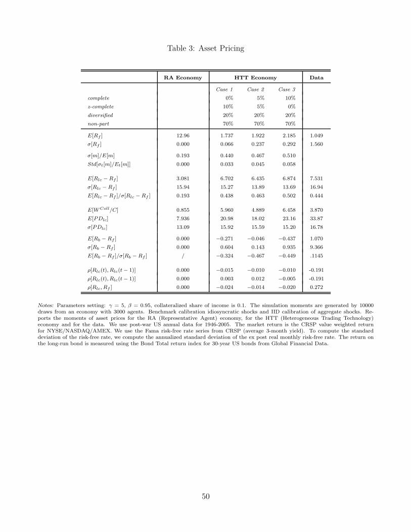
Table 3: Asset Pricing

RA Economy HTT Economy Data

Case 1 Case 2 Case 3

complete 0% 5% 10%

z-complete 10% 5% 0%

diversified 20% 20% 20%

non-part 70% 70% 70%

E[Rf ] 12.96 1.737 1.922 2.185 1.049

σ[Rf ] 0.000 0.066 0.237 0.292 1.560

σ[m]/E[m] 0.193 0.440 0.467 0.510

Std[σt[m]/Et[m]] 0.000 0.033 0.045 0.058

E[Rlc − Rf ] 3.081 6.702 6.435 6.874 7.531

σ[Rlc − Rf ] 15.94 15.27 13.89 13.69 16.94

E[Rlc − Rf ]/σ[Rlc − Rf ] 0.193 0.438 0.463 0.502 0.444

E[W Coll/C] 0.855 5.960 4.889 6.458 3.870

E[PDlc] 7.936 20.98 18.02 23.16 33.87

σ[PDlc] 13.09 15.92 15.59 15.20 16.78

E[Rb − Rf ] 0.000 −0.271 −0.046 −0.437 1.070

σ[Rb − Rf ] 0.000 0.604 0.143 0.935 9.366

E[Rb − Rf ]/σ[Rb − Rf ] / −0.324 −0.467 −0.449 .1145

ρ[Rlc(t), Rlc(t − 1)] 0.000 −0.015 −0.010 −0.010 -0.191

ρ[Rlc(t), Rlc(t − 1)] 0.000 0.003 0.012 −0.005 -0.191

ρ[Rlc, Rf ] 0.000 −0.024 −0.014 −0.020 0.272

Notes: Parameters setting: γ = 5, β = 0.95, collateralized share of income is 0.1. The simulation moments are generated by 10000draws from an economy with 3000 agents. Benchmark calibration idiosyncratic shocks and IID calibration of aggregate shocks. Re-ports the moments of asset prices for the RA (Representative Agent) economy, for the HTT (Heterogeneous Trading Technology)economy and for the data. We use post-war US annual data for 1946-2005. The market return is the CRSP value weighted returnfor NYSE/NASDAQ/AMEX. We use the Fama risk-free rate series from CRSP (average 3-month yield). To compute the standarddeviation of the risk-free rate, we compute the annualized standard deviation of the ex post real monthly risk-free rate. The return onthe long-run bond is measured using the Bond Total return index for 30-year US bonds from Global Financial Data.

50

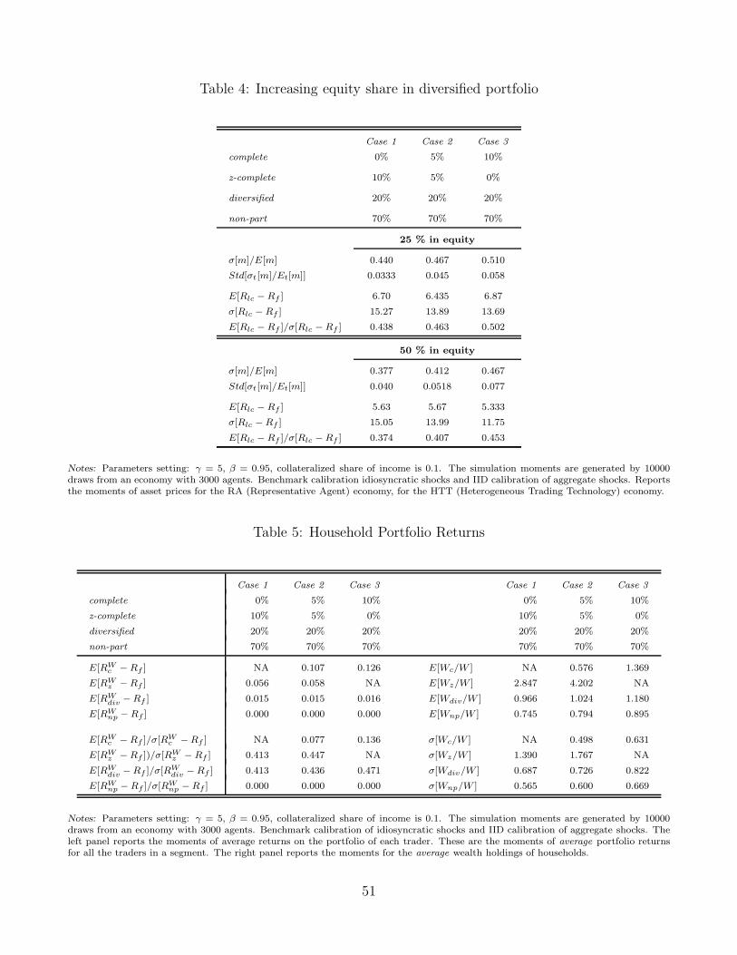
Table 4: Increasing equity share in diversified portfolio

Case 1 Case 2 Case 3

complete 0% 5% 10%

z-complete 10% 5% 0%

diversified 20% 20% 20%

non-part 70% 70% 70%

25 % in equity

σ[m]/E[m] 0.440 0.467 0.510

Std[σt[m]/Et[m]] 0.0333 0.045 0.058

E[Rlc − Rf ] 6.70 6.435 6.87

σ[Rlc − Rf ] 15.27 13.89 13.69

E[Rlc − Rf ]/σ[Rlc − Rf ] 0.438 0.463 0.502

50 % in equity

σ[m]/E[m] 0.377 0.412 0.467

Std[σt[m]/Et[m]] 0.040 0.0518 0.077

E[Rlc − Rf ] 5.63 5.67 5.333

σ[Rlc − Rf ] 15.05 13.99 11.75

E[Rlc − Rf ]/σ[Rlc − Rf ] 0.374 0.407 0.453

Notes: Parameters setting: γ = 5, β = 0.95, collateralized share of income is 0.1. The simulation moments are generated by 10000draws from an economy with 3000 agents. Benchmark calibration idiosyncratic shocks and IID calibration of aggregate shocks. Reportsthe moments of asset prices for the RA (Representative Agent) economy, for the HTT (Heterogeneous Trading Technology) economy.

Table 5: Household Portfolio Returns

Case 1 Case 2 Case 3 Case 1 Case 2 Case 3

complete 0% 5% 10% 0% 5% 10%

z-complete 10% 5% 0% 10% 5% 0%

diversified 20% 20% 20% 20% 20% 20%

non-part 70% 70% 70% 70% 70% 70%

E[RWc − Rf ] NA 0.107 0.126 E[Wc/W ] NA 0.576 1.369

E[RWz − Rf ] 0.056 0.058 NA E[Wz/W ] 2.847 4.202 NA

E[RWdiv − Rf ] 0.015 0.015 0.016 E[Wdiv/W ] 0.966 1.024 1.180

E[RWnp − Rf ] 0.000 0.000 0.000 E[Wnp/W ] 0.745 0.794 0.895

E[RWc − Rf ]/σ[RW

c − Rf ] NA 0.077 0.136 σ[Wc/W ] NA 0.498 0.631

E[RWz − Rf ])/σ[RW

z − Rf ] 0.413 0.447 NA σ[Wz/W ] 1.390 1.767 NA

E[RWdiv − Rf ]/σ[RW

div − Rf ] 0.413 0.436 0.471 σ[Wdiv/W ] 0.687 0.726 0.822

E[RWnp − Rf ]/σ[RW

np − Rf ] 0.000 0.000 0.000 σ[Wnp/W ] 0.565 0.600 0.669

Notes: Parameters setting: γ = 5, β = 0.95, collateralized share of income is 0.1. The simulation moments are generated by 10000draws from an economy with 3000 agents. Benchmark calibration of idiosyncratic shocks and IID calibration of aggregate shocks. Theleft panel reports the moments of average returns on the portfolio of each trader. These are the moments of average portfolio returnsfor all the traders in a segment. The right panel reports the moments for the average wealth holdings of households.

51

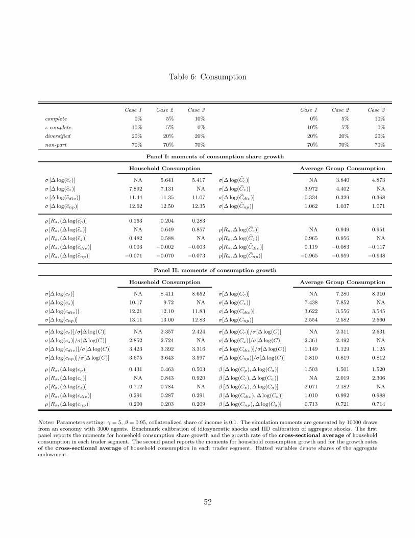
Table 6: Consumption

Case 1 Case 2 Case 3 Case 1 Case 2 Case 3

complete 0% 5% 10% 0% 5% 10%

z-complete 10% 5% 0% 10% 5% 0%

diversified 20% 20% 20% 20% 20% 20%

non-part 70% 70% 70% 70% 70% 70%

Panel I: moments of consumption share growth

Household Consumption Average Group Consumption

σ [∆ log(cc)] NA 5.641 5.417 σ[∆ log(Cc)] NA 3.840 4.873

σ [∆ log(cz)] 7.892 7.131 NA σ[∆ log(Cz)] 3.972 4.402 NA

σ [∆ log(cdiv)] 11.44 11.35 11.07 σ[∆ log(Cdiv)] 0.334 0.329 0.368

σ [∆ log(cnp)] 12.62 12.50 12.35 σ[∆ log(Cnp)] 1.062 1.037 1.071

ρ [Rs, (∆ log(cp)] 0.163 0.204 0.283

ρ [Rs, (∆ log(cc)] NA 0.649 0.857 ρ[Rs, ∆log(Cc)] NA 0.949 0.951

ρ [Rs, (∆ log(cz)] 0.482 0.588 NA ρ[Rs, ∆log(Cz)] 0.965 0.956 NA

ρ [Rs, (∆ log(cdiv)] 0.003 −0.002 −0.003 ρ[Rs, ∆log(Cdiv)] 0.119 −0.083 −0.117

ρ [Rs, (∆ log(cnp)] −0.071 −0.070 −0.073 ρ[Rs, ∆log(Cnp)] −0.965 −0.959 −0.948

Panel II: moments of consumption growth

Household Consumption Average Group Consumption

σ[∆ log(cc)] NA 8.411 8.652 σ[∆ log(Cc)] NA 7.280 8.310

σ[∆ log(cz)] 10.17 9.72 NA σ[∆ log(Cz)] 7.438 7.852 NA

σ[∆ log(cdiv)] 12.21 12.10 11.83 σ[∆ log(Cdiv)] 3.622 3.556 3.545

σ[∆ log(cnp)] 13.11 13.00 12.83 σ[∆ log(Cnp)] 2.554 2.582 2.560

σ[∆ log(cc)]/σ[∆ log(C)] NA 2.357 2.424 σ[∆ log(Cc)]/σ[∆ log(C)] NA 2.311 2.631

σ[∆ log(cz)]/σ[∆ log(C)] 2.852 2.724 NA σ[∆ log(Cz)]/σ[∆ log(C)] 2.361 2.492 NA

σ[∆ log(cdiv)]/σ[∆ log(C)] 3.423 3.392 3.316 σ[∆ log(Cdiv)]/σ[∆ log(C)] 1.149 1.129 1.125

σ[∆ log(cnp)]/σ[∆ log(C)] 3.675 3.643 3.597 σ[∆ log(Cnp)]/σ[∆ log(C)] 0.810 0.819 0.812

ρ [Rs, (∆ log(cp)] 0.431 0.463 0.503 β [∆ log(Cp), ∆log(Ca)] 1.503 1.501 1.520

ρ [Rs, (∆ log(cc)] NA 0.843 0.920 β [∆ log(Cc), ∆log(Ca)] NA 2.019 2.306

ρ [Rs, (∆ log(cz)] 0.712 0.784 NA β [∆ log(Cz),∆ log(Ca)] 2.071 2.182 NA

ρ [Rs, (∆ log(cdiv)] 0.291 0.287 0.291 β [∆ log(Cdiv), ∆log(Ca)] 1.010 0.992 0.988

ρ [Rs, (∆ log(cnp)] 0.200 0.203 0.209 β [∆ log(Cnp), ∆ log(Ca)] 0.713 0.721 0.714

Notes: Parameters setting: γ = 5, β = 0.95, collateralized share of income is 0.1. The simulation moments are generated by 10000 drawsfrom an economy with 3000 agents. Benchmark calibration of idiosyncratic shocks and IID calibration of aggregate shocks. The firstpanel reports the moments for household consumption share growth and the growth rate of the cross-sectional average of householdconsumption in each trader segment. The second panel reports the moments for household consumption growth and for the growth ratesof the cross-sectional average of household consumption in each trader segment. Hatted variables denote shares of the aggregateendowment.

52

Table 7: Matching Income Distribution

Percentile Ratio Model US Data

75/50 2.739 1.785

80/50 2.893 2.041

85/50 3.062 2.414

90/50 3.353 2.908

75/25 4.136 3.449

80/25 4.369 3.943

85/25 4.624 4.663

90/25 5.063 5.618

80/20 4.613 4.710

85/15 6.537 7.024

90/10 11.42 11.64

Notes: Parameters setting: γ = 5, β = 0.95, collateralized share of income is 0.1. The simulation moments are generated by 10000draws from an economy with 3000 agents. Benchmark calibration of aggregate and idiosyncratic shocks. The income data are from the2004 SCF.

Table 8: Household Wealth Distribution

Bewley Model HTT Model US Data 2004

Wealth Wealth Net Worth Total Assets

Standard Twisted Standard Twisted

kurtosis 1.96 2.84 6.97 12.92 15.87 48.85

skewness 0.23 0.88 1.80 2.73 3.616 6.250

Gini 0.40 0.48 0.53 0.57 0.793 0.697

Percentile Ratio

W75/W25 4.03 5.42 6.37 6.90 25.09 10.64

W80/W20 6.38 9.09 11.28 12.49 65.41 33.42

W85/W15 12.63 19.12 26.11 29.85 211.9 55.75

W90/W10 48.14 82.20 182.64 240.5 999.1 580.5

W50/W10 23.18 25.33 53.32 65.02 105.0 91.00

W90/W50 2.077 3.22 3.42 3.69 9.510 6.378

Notes: Parameters setting: γ = 5, β = 0.95, collateralized share of income is 0.1. The simulation moments are generated by 10000 drawsfrom an economy with 3000 agents. Benchmark calibration of idiosyncratic shocks and aggregate shocks. The wealth data are from the2004 SCF. The HTT model has 10% z-complete traders, 20% diversified traders and 70 % non-participants. The Bewley model has100% diversified traders.

53

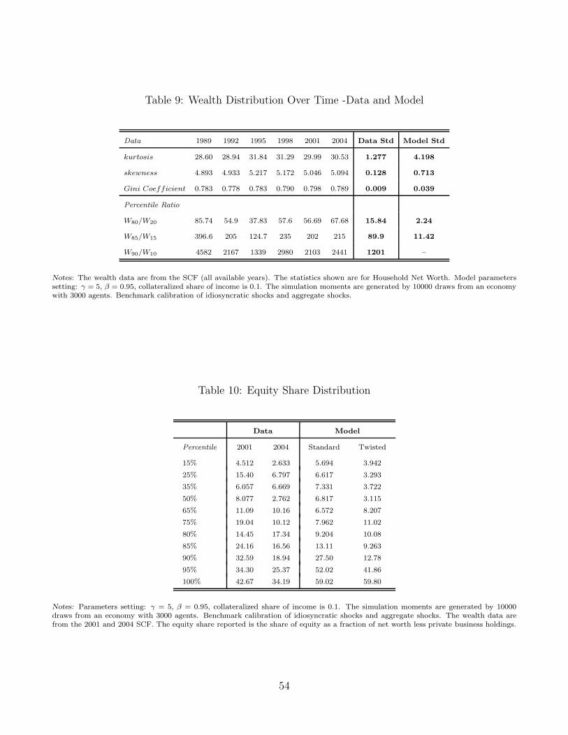
Table 9: Wealth Distribution Over Time -Data and Model

Data 1989 1992 1995 1998 2001 2004 Data Std Model Std

kurtosis 28.60 28.94 31.84 31.29 29.99 30.53 1.277 4.198

skewness 4.893 4.933 5.217 5.172 5.046 5.094 0.128 0.713

Gini Coefficient 0.783 0.778 0.783 0.790 0.798 0.789 0.009 0.039

Percentile Ratio

W80/W20 85.74 54.9 37.83 57.6 56.69 67.68 15.84 2.24

W85/W15 396.6 205 124.7 235 202 215 89.9 11.42

W90/W10 4582 2167 1339 2980 2103 2441 1201 –

Notes: The wealth data are from the SCF (all available years). The statistics shown are for Household Net Worth. Model parameterssetting: γ = 5, β = 0.95, collateralized share of income is 0.1. The simulation moments are generated by 10000 draws from an economywith 3000 agents. Benchmark calibration of idiosyncratic shocks and aggregate shocks.

Table 10: Equity Share Distribution

Data Model

Percentile 2001 2004 Standard Twisted

15% 4.512 2.633 5.694 3.942

25% 15.40 6.797 6.617 3.293

35% 6.057 6.669 7.331 3.722

50% 8.077 2.762 6.817 3.115

65% 11.09 10.16 6.572 8.207

75% 19.04 10.12 7.962 11.02

80% 14.45 17.34 9.204 10.08

85% 24.16 16.56 13.11 9.263

90% 32.59 18.94 27.50 12.78

95% 34.30 25.37 52.02 41.86

100% 42.67 34.19 59.02 59.80

Notes: Parameters setting: γ = 5, β = 0.95, collateralized share of income is 0.1. The simulation moments are generated by 10000draws from an economy with 3000 agents. Benchmark calibration of idiosyncratic shocks and aggregate shocks. The wealth data arefrom the 2001 and 2004 SCF. The equity share reported is the share of equity as a fraction of net worth less private business holdings.

54

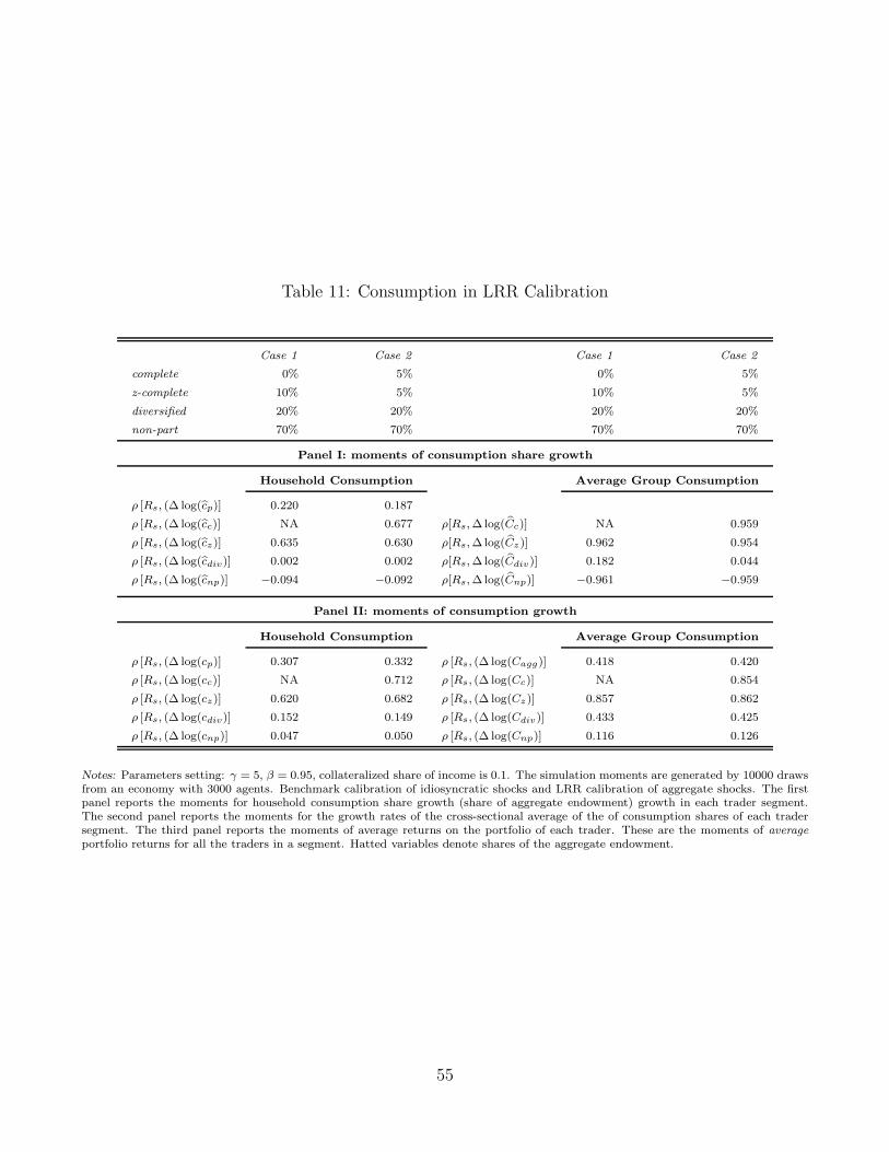
Table 11: Consumption in LRR Calibration

Case 1 Case 2 Case 1 Case 2

complete 0% 5% 0% 5%

z-complete 10% 5% 10% 5%

diversified 20% 20% 20% 20%

non-part 70% 70% 70% 70%

Panel I: moments of consumption share growth

Household Consumption Average Group Consumption

ρ [Rs, (∆ log(cp)] 0.220 0.187

ρ [Rs, (∆ log(cc)] NA 0.677 ρ[Rs, ∆log(Cc)] NA 0.959

ρ [Rs, (∆ log(cz)] 0.635 0.630 ρ[Rs, ∆log(Cz)] 0.962 0.954

ρ [Rs, (∆ log(cdiv)] 0.002 0.002 ρ[Rs, ∆log(Cdiv)] 0.182 0.044

ρ [Rs, (∆ log(cnp)] −0.094 −0.092 ρ[Rs, ∆log(Cnp)] −0.961 −0.959

Panel II: moments of consumption growth

Household Consumption Average Group Consumption

ρ [Rs, (∆ log(cp)] 0.307 0.332 ρ [Rs, (∆ log(Cagg)] 0.418 0.420

ρ [Rs, (∆ log(cc)] NA 0.712 ρ [Rs, (∆ log(Cc)] NA 0.854

ρ [Rs, (∆ log(cz)] 0.620 0.682 ρ [Rs, (∆ log(Cz)] 0.857 0.862

ρ [Rs, (∆ log(cdiv)] 0.152 0.149 ρ [Rs, (∆ log(Cdiv)] 0.433 0.425

ρ [Rs, (∆ log(cnp)] 0.047 0.050 ρ [Rs, (∆ log(Cnp)] 0.116 0.126

Notes: Parameters setting: γ = 5, β = 0.95, collateralized share of income is 0.1. The simulation moments are generated by 10000 drawsfrom an economy with 3000 agents. Benchmark calibration of idiosyncratic shocks and LRR calibration of aggregate shocks. The firstpanel reports the moments for household consumption share growth (share of aggregate endowment) growth in each trader segment.The second panel reports the moments for the growth rates of the cross-sectional average of the of consumption shares of each tradersegment. The third panel reports the moments of average returns on the portfolio of each trader. These are the moments of average

portfolio returns for all the traders in a segment. Hatted variables denote shares of the aggregate endowment.

55

Figure 1: Conditional Risk Premium and Market Price of Risk

50 55 60 65 70 75 80 85 90 95 100

h’/h shocks

1

1.5

2

50 55 60 65 70 75 80 85 90 95 100

Conditional Risk Premium

0.04

0.06

0.08

Conditional market price of risk

50 55 60 65 70 75 80 85 90 95 1000.35

0.55

0.7

Notes: Market Segmentation: 5% complete, 5% in z-complete, 20% diversified and 70% non-participants. Parameters setting: γ = 5,

β = 0.95, collateralized share of income is 0.1. Plot of 50 draws from an economy with 3000 agents. Benchmark calibration of

idiosyncratic shocks and IID calibration of idiosyncratic shocks. The shaded are indicates low aggregate consumption growth states.

Figure 2: Equity Share

50 55 60 65 70 75 80 85 90 95 100

Net Wealth/C

50 55 60 65 70 75 80 85 90 95 10030

40

50

60

50 55 60 65 70 75 80 85 90 95 100

Portfolio Share of Equity

50 55 60 65 70 75 80 85 90 95 1000.5

1

1.5

50 55 60 65 70 75 80 85 90 95 100

Conditional Market Price of Risk

50 55 60 65 70 75 80 85 90 95 1000.4

0.5

0.6

0.7

Notes: Market Segmentation: 5% complete, 5% in z-complete, 20% diversified and 70% non-participants. Parameters setting: γ = 5,

β = 0.95, collateralized share of income is 0.1. The simulation moments are generated by 100 draws from an economy with 3000 agents.

Benchmark calibration of idiosyncratic and IID calibration of aggregate shocks. The shaded areas indicate low aggregate consumption

growth states.

56

Figure 3: Equity Share

0 0.2 0.4 0.6 0.8 1 1.2 1.4 1.6 1.8 20

2

4

6

8

10

12

14

16

18

20

Fraction of equity in portfolio

Percen

tage o

f consu

mption

Welfare Loss

Case 1Case 2Case 3

Notes: Parameters setting: γ = 5, β = 0.95, collateralized share of income is 0.1 . The simulation moments are generated by 100

draws from an economy with 3000 agents. Benchmark calibration of idiosyncratic shocks and aggregate shocks. Case 1: 0/10/20

(complete/z-complete/diversified) composition of trader segments. Case 2: 5/5/20 composition. Case 3: 10/0/20 composition.

57