A multiple testing approach to the regularisation of large ... · A multiple testing approach to the regularisation of large sample correlation matrices ... (Fan et al. (2008)) and

A multiple testing approach to the regularisation oflarge sample correlation matrices�

Natalia BaileyQueen Mary, University of London

M. Hashem PesaranUniversity of Southern California, USA, and Trinity College, Cambridge

L. Vanessa SmithUniversity of York

November 5, 2015

Abstract

This paper proposes a regularisation method for the estimation of large covariancematrices that uses insights from the multiple testing (MT ) literature. The approachtests the statistical signi�cance of individual pair-wise correlations and sets to zerothose elements that are not statistically signi�cant, taking account of the multipletesting nature of the problem. By using the inverse of the normal distribution at apredetermined signi�cance level, it circumvents the challenge of estimating the theoret-ical constant arising in the rate of convergence of existing thresholding estimators, andhence it is easy to implement and does not require cross-validation. TheMT estimatorof the sample correlation matrix is shown to be consistent in the spectral and Frobe-nius norms, and in terms of support recovery, so long as the true covariance matrix issparse. The performance of the proposed MT estimator is compared to a number ofother estimators in the literature using Monte Carlo experiments. It is shown that theMT estimator performs well and tends to outperform the other estimators, particularlywhen the cross section dimension, N , is larger than the time series dimension, T:

JEL Classi�cations: C13, C58Keywords: Sparse correlation matrices, High-dimensional data, Multiple testing,

Thresholding, Shrinkage

�The authors would like to thank Alex Chudik, Jianqing Fan, George Kapetanios, Yuan Liao, Ron Smithand Michael Wolf for valuable comments and suggestions, as well as Elizaveta Levina and Martina Minchevafor helpful email correspondence with regard to implementation of their approaches. The authors also wishto acknowledge �nancial support under ESRC Grant ES/I031626/1.

1 Introduction

Improved estimation of covariance matrices is a problem that features prominently in anumber of areas of multivariate statistical analysis. In �nance it arises in portfolio selectionand optimisation (Ledoit and Wolf (2003)), risk management (Fan et al. (2008)) and testingof capital asset pricing models (Sentana (2009)). In global macro-econometric modellingwith many domestic and foreign channels of interactions, error covariance matrices must beestimated for impulse response analysis and bootstrapping (Pesaran et al. (2004); Dees etal. (2007)). In the area of bio-informatics, covariance matrices are required when inferringgene association networks (Carroll (2003); Schäfer and Strimmer (2005)). Such matrices arefurther encountered in �elds including meteorology, climate research, spectroscopy, signalprocessing and pattern recognition.Importantly, the issue of consistently estimating the population covariance matrix, � =

(�ij), becomes particularly challenging when the number of variables, N , is larger than thenumber of observations, T . In this case, one way of obtaining a suitable estimator for �is to appropriately restrict the o¤-diagonal elements of its sample estimate denoted by �.Numerous methods have been developed to address this challenge, predominantly in thestatistics literature. See Pourahmadi (2011) for an extensive review and references therein.Some approaches are regression-based and make use of suitable decompositions of � such asthe Cholesky decomposition (see Pourahmadi (1999, 2000), Rothman et al. (2010), Abadiret al. (2014), among others). Others include banding or tapering methods as proposed, forexample, by Bickel and Levina (2004, 2008a) and Wu and Pourahmadi (2009), which assumethat the variables under consideration follow a natural ordering. Two popular regularisationtechniques in the literature that do not make use of any ordering assumptions are those ofthresholding and shrinkage.Thresholding involves setting o¤-diagonal elements of the sample covariance matrix that

are in absolute terms below certain threshold values to zero. This approach includes �uni-versal�thresholding put forward by El Karoui (2008) and Bickel and Levina (2008b), and�adaptive�thresholding proposed by Cai and Liu (2011). Universal thresholding applies thesame thresholding parameter to all o¤-diagonal elements of the unconstrained sample co-variance matrix, while adaptive thresholding allows the threshold value to vary across thedi¤erent o¤-diagonal elements of the matrix. Furthermore, the selected non-zero elementsof � can either be set to their sample estimates or can be adjusted downward. This relatesto the concepts of �hard�and �soft�thresholding, respectively. The thresholding approachtraditionally assumes that the underlying (population) covariance matrix is sparse, wheresparseness is loosely de�ned as the presence of a su¢ cient number of zeros on each rowof � such that it is absolute summable row (column)-wise, or more generally in the sensede�ned by El Karoui (2008). However, Fan et al. (2011, 2013) show that such regularisationtechniques can be applied even if the underlying population covariance matrix is not sparse,so long as the non-sparseness is characterised by an approximate factor structure. The mainchallenge in applying this approach lies in the estimation of the thresholding parameter.The method of cross-validation is primarily used for this purpose which has its own limita-

1

tions and may not be appropriate in applications where the underlying model generating theobservations is unstable over time.In contrast to thresholding, the shrinkage approach reduces all sample estimates of the

covariance matrix towards zero element-wise. More formally, the shrinkage estimator of � isde�ned as a weighted average of the sample covariance matrix and an invertible covariancematrix estimator known as the shrinkage target - see Friedman (1989). A number of shrinkagetargets have been considered in the literature that take advantage of a priori knowledge ofthe data characteristics under investigation. Examples of covariance matrix targets can befound in Ledoit and Wolf (2003), Daniels and Kass (1999, 2001), Fan et al. (2008), andHo¤ (2009), among others. Ledoit and Wolf (2004) suggest a modi�ed shrinkage estimatorthat involves a linear combination of the unrestricted sample covariance matrix with theidentity matrix. This is recommended by the authors for more general situations where nonatural shrinking target exists. On the whole, shrinkage estimators tend to be stable, butyield inconsistent estimates if the purpose of the analysis is the estimation of the true andfalse positive rates of the underlying true sparse covariance matrix (the so called �supportrecovery�problem).This paper considers an alternative to cross-validation by making use of a multiple testing

(MT ) approach to set the thresholding parameter. The idea has been suggested by ElKaroui (2008, p. 2748) but has not been theoretically developed in the literature. Asnoted by El Karoui, hard thresholding can also be implemented by testing the N(N � 1)=2null hypotheses that �ij = 0, for all i 6= j. However, such tests will not be standard andtheir critical value must be determined from the knowledge of the inferential problem andthe fact that N and T both tend to in�nity. The MT approach can readily accommodateboth Gaussian and non-Gaussian observations and does not require cross-validation whichis often quite time consuming to apply. The MT procedure is shown to be equivalent tothe application of the multiple testing procedure due to Bonferroni (1935) to the individualrows of �, separately, when �ij = 0 implies independence, and to all distinct non-diagonalelements of �, if �ij = 0 does not imply independence. We show that the MT estimatorof R, the correlation matrix associated with �, converges in spectral norm at the rate ofOp

�mNpT

�, where mN is the maximum number of non-zero elements in the o¤-diagonal rows

of R. This compares favourably with the corresponding Op

�mN

qlog(N)T

�rate established

in the literature. Similarly, we show that the MT estimator converges in Frobenius norm

at the rate of Op

�qmNNT

�, even if the underlying observations are non-Gaussian. To

the best of our knowledge, the only work that addresses the theoretical properties of thethresholding estimator for the Frobenius norm is Bickel and Levina (2008b), who establish the

rate of Op

�qmNN log(N)

T

�, assuming the observations are Gaussian. TheMT estimator also

consistently recovers the support of the population covariance matrix under non-Gaussianobservations.The performance of the MT estimator is investigated using a Monte Carlo simulation

2

study, and its properties are compared to a number of extant regularised estimators inthe literature. The simulation results show that the proposed multiple testing estimator isrobust to the typical choices of p used in the literature (10%, 5% and 1%), and performsfavourably compared to the other estimators, especially when N is large relative to T . TheMT procedure also dominates other regularised estimators when the focus of the analysis ison support recovery.The rest of the paper is organised as follows: Section 2 outlines some preliminaries,

introduces the MT procedure and derives its asymptotic properties. The small sampleproperties of the MT estimator are investigated in Section 3. Concluding remarks areprovided in Section 4. Some of the technical proofs and additional simulation results areprovided in a Supplementary Appendix.Notation: We denote the largest and the smallest eigenvalues of theN�N real symmetric

matrix A = (aij) by �max (A) and �min (A) ; respectively, its trace by tr (A) =PN

i=1 aii, its

maximum absolute column sum norm by kAk1 = max1�j�N

�PNi=1 jaijj

�, its maximum

absolute row sum norm by kAk1 = max1�i�N

�PNj=1 jaijj

�, its spectral radius by % (A) =

j�max (A)j, its spectral (or operator) norm by kAkspec = �1=2max (A0A), its Frobenius norm

by kAkF =ptr (A0A). Note that kAkspec = % (A). aN = O(bN) states the deterministic

sequence faNg is at most of order bN , xN = Op(yN) states the vector of random variables,xN ; is at most of order yN in probability, and xN = op(yN) is of smaller order in probabilitythan yN , !p denotes convergence in probability, and !d convergence in distribution. Allasymptotics are carried out under N !1 jointly with T !1.

2 Regularising the sample correlation matrix: A mul-tiple testing (MT) approach

Let fxit; i 2 N; t 2 Tg, N � N; T � Z, be a double index process where xit is de-�ned on a suitable probability space (; F; P ), and denote the covariance matrix of xt =(x1t; x2t; :::; xNt)

0 byV ar (xt) = � = E

�(xt � �) (xt � �)0

�; (1)

where E(xt) = � = (�1; �2; :::; �N)0, and � is an N � N symmetric, positive de�nite real

matrix with (i; j) element, �ij.We consider the regularisation of the sample covariance matrix estimator of �, denoted

by �, with elements

�ij;T = T�1TXt=1

(xit � �xi) (xjt � �xj) ; for i; j = 1; 2; :::; N; (2)

where �xi = T�1PT

t=1 xit. To this end we assume that � is (exactly) sparse de�ned as follows.

3

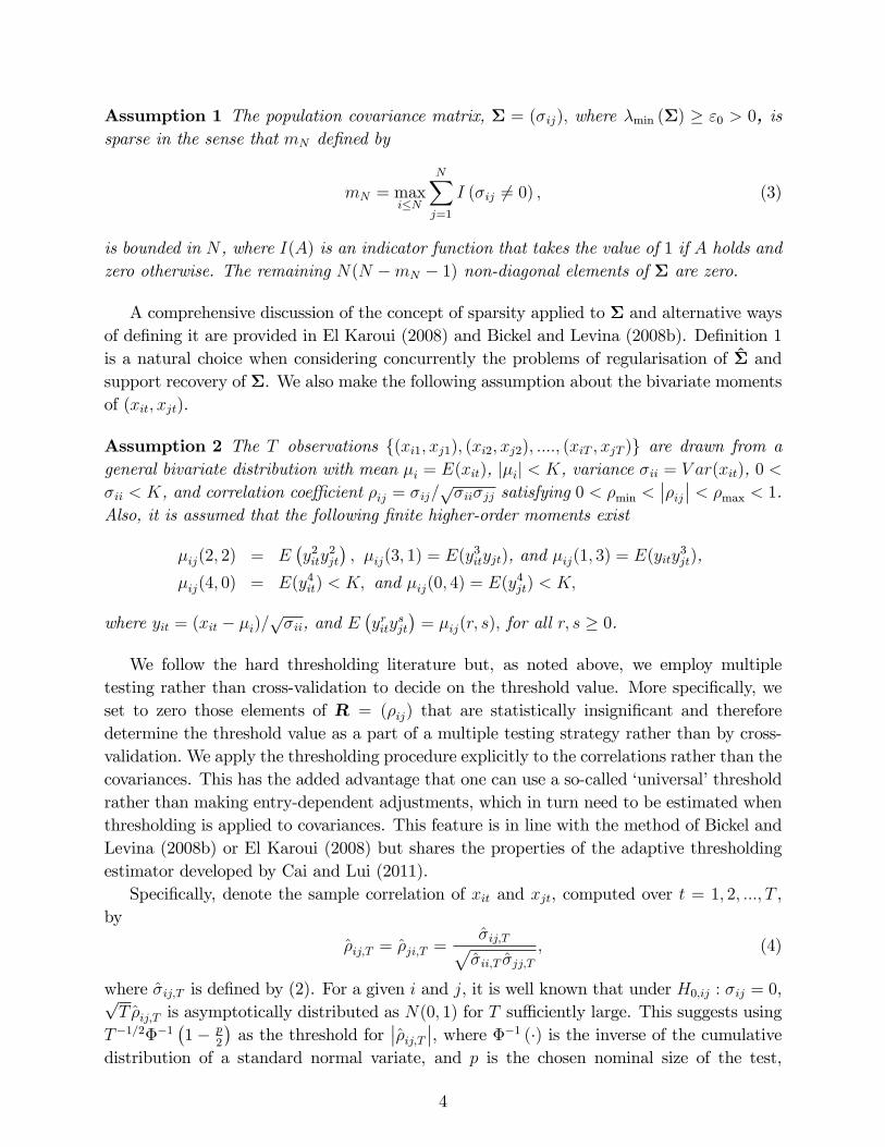
Assumption 1 The population covariance matrix, � = (�ij); where �min (�) � "0 > 0, issparse in the sense that mN de�ned by

mN = maxi�N

NXj=1

I (�ij 6= 0) ; (3)

is bounded in N , where I(A) is an indicator function that takes the value of 1 if A holds andzero otherwise. The remaining N(N �mN � 1) non-diagonal elements of � are zero.

A comprehensive discussion of the concept of sparsity applied to � and alternative waysof de�ning it are provided in El Karoui (2008) and Bickel and Levina (2008b). De�nition 1is a natural choice when considering concurrently the problems of regularisation of � andsupport recovery of �. We also make the following assumption about the bivariate momentsof (xit; xjt).

Assumption 2 The T observations f(xi1; xj1); (xi2; xj2); ::::; (xiT ; xjT )g are drawn from ageneral bivariate distribution with mean �i = E(xit), j�ij < K, variance �ii = V ar(xit), 0 <�ii < K, and correlation coe¢ cient �ij = �ij=

p�ii�jj satisfying 0 < �min <

��ij�� < �max < 1.Also, it is assumed that the following �nite higher-order moments exist

�ij(2; 2) = E�y2ity

2jt

�; �ij(3; 1) = E(y3ityjt), and �ij(1; 3) = E(yity

3jt),

�ij(4; 0) = E(y4it) < K; and �ij(0; 4) = E(y4jt) < K;

where yit = (xit � �i)=p�ii, and E

�yrity

sjt

�= �ij(r; s); for all r; s � 0.

We follow the hard thresholding literature but, as noted above, we employ multipletesting rather than cross-validation to decide on the threshold value. More speci�cally, weset to zero those elements of R = (�ij) that are statistically insigni�cant and thereforedetermine the threshold value as a part of a multiple testing strategy rather than by cross-validation. We apply the thresholding procedure explicitly to the correlations rather than thecovariances. This has the added advantage that one can use a so-called �universal�thresholdrather than making entry-dependent adjustments, which in turn need to be estimated whenthresholding is applied to covariances. This feature is in line with the method of Bickel andLevina (2008b) or El Karoui (2008) but shares the properties of the adaptive thresholdingestimator developed by Cai and Lui (2011).Speci�cally, denote the sample correlation of xit and xjt, computed over t = 1; 2; :::; T ,

by

�ij;T = �ji;T =�ij;Tp�ii;T �jj;T

; (4)

where �ij;T is de�ned by (2). For a given i and j, it is well known that under H0;ij : �ij = 0,pT �ij;T is asymptotically distributed as N(0; 1) for T su¢ ciently large. This suggests using

T�1=2��1�1� p

2

�as the threshold for

��ij;T ��, where ��1 (�) is the inverse of the cumulativedistribution of a standard normal variate, and p is the chosen nominal size of the test,

4

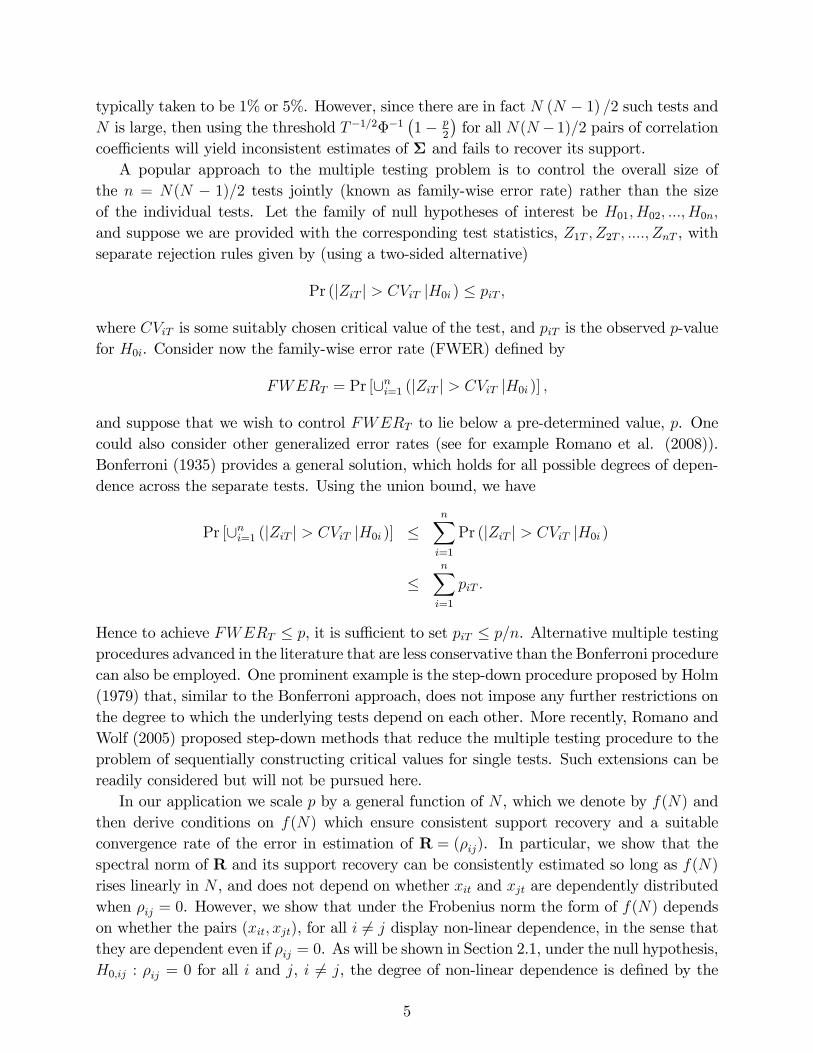
typically taken to be 1% or 5%. However, since there are in fact N (N � 1) =2 such tests andN is large, then using the threshold T�1=2��1

�1� p

2

�for all N(N �1)=2 pairs of correlation

coe¢ cients will yield inconsistent estimates of � and fails to recover its support.A popular approach to the multiple testing problem is to control the overall size of

the n = N(N � 1)=2 tests jointly (known as family-wise error rate) rather than the sizeof the individual tests. Let the family of null hypotheses of interest be H01; H02; :::; H0n;

and suppose we are provided with the corresponding test statistics, Z1T ; Z2T ; ::::; ZnT , withseparate rejection rules given by (using a two-sided alternative)

Pr (jZiT j > CViT jH0i ) � piT ;

where CViT is some suitably chosen critical value of the test, and piT is the observed p-valuefor H0i. Consider now the family-wise error rate (FWER) de�ned by

FWERT = Pr [[ni=1 (jZiT j > CViT jH0i )] ;

and suppose that we wish to control FWERT to lie below a pre-determined value, p. Onecould also consider other generalized error rates (see for example Romano et al. (2008)).Bonferroni (1935) provides a general solution, which holds for all possible degrees of depen-dence across the separate tests. Using the union bound, we have

Pr [[ni=1 (jZiT j > CViT jH0i )] �nXi=1

Pr (jZiT j > CViT jH0i )

�nXi=1

piT :

Hence to achieve FWERT � p, it is su¢ cient to set piT � p=n. Alternative multiple testingprocedures advanced in the literature that are less conservative than the Bonferroni procedurecan also be employed. One prominent example is the step-down procedure proposed by Holm(1979) that, similar to the Bonferroni approach, does not impose any further restrictions onthe degree to which the underlying tests depend on each other. More recently, Romano andWolf (2005) proposed step-down methods that reduce the multiple testing procedure to theproblem of sequentially constructing critical values for single tests. Such extensions can bereadily considered but will not be pursued here.In our application we scale p by a general function of N , which we denote by f(N) and

then derive conditions on f(N) which ensure consistent support recovery and a suitableconvergence rate of the error in estimation of R = (�ij). In particular, we show that thespectral norm of R and its support recovery can be consistently estimated so long as f(N)rises linearly in N , and does not depend on whether xit and xjt are dependently distributedwhen �ij = 0. However, we show that under the Frobenius norm the form of f(N) dependson whether the pairs (xit; xjt), for all i 6= j display non-linear dependence, in the sense thatthey are dependent even if �ij = 0. As will be shown in Section 2.1, under the null hypothesis,H0;ij : �ij = 0 for all i and j, i 6= j, the degree of non-linear dependence is de�ned by the

5

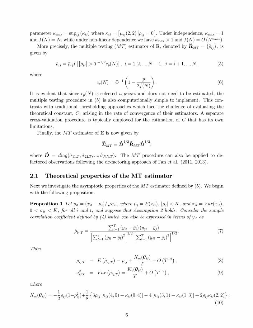
parameter �max = supij (�ij) where �ij =��ij(2; 2)

��ij = 0�. Under independence, �max = 1and f(N) = N , while under non-linear dependence we have �max > 1 and f(N) = O (N�max).More precisely, the multiple testing (MT ) estimator of R, denoted by eRMT =

�~�ij�; is

given by

~�ij = �ijI��ij�� > T�1=2cp(N)

�; i = 1; 2; :::; N � 1; j = i+ 1; :::; N; (5)

where

cp(N) = ��1�1� p

2f(N)

�: (6)

It is evident that since cp(N) is selected a priori and does not need to be estimated, themultiple testing procedure in (5) is also computationally simple to implement. This con-trasts with traditional thresholding approaches which face the challenge of evaluating thetheoretical constant, C, arising in the rate of convergence of their estimators. A separatecross-validation procedure is typically employed for the estimation of C that has its ownlimitations.Finally, the MT estimator of � is now given by

e�MT = D1=2 eRMTD

1=2;

where D = diag(�11;T ; �22;T ; :::; �NN;T ). The MT procedure can also be applied to de-factored observations following the de-factoring approach of Fan et al. (2011, 2013).

2.1 Theoretical properties of the MT estimator

Next we investigate the asymptotic properties of theMT estimator de�ned by (5). We beginwith the following proposition.

Proposition 1 Let yit = (xit � �i)=p�ii, where �i = E(xit), j�ij < K, and �ii = V ar(xit),

0 < �ii < K, for all i and t, and suppose that Assumption 2 holds. Consider the samplecorrelation coe¢ cient de�ned by (4) which can also be expressed in terms of yit as

�ij;T =

PTt=1 (yit � �yi) (yjt � �yj)hPT

t=1 (yit � �yi)2i1=2 hPT

t=1 (yjt � �yj)2i1=2 : (7)

Then

�ij;T = E��ij;T

�= �ij +

Km(�ij)

T+O

�T�2

�; (8)

!2ij;T = V ar��ij;T

�=Kv(�ij)

T+O

�T�2

�; (9)

where

Km(�ij) = �1

2�ij(1��2ij)+

1

8

�3�ij [�ij(4; 0) + �ij(0; 4)]� 4 [�ij(3; 1) + �ij(1; 3)] + 2�ij�ij(2; 2)

;

(10)

6

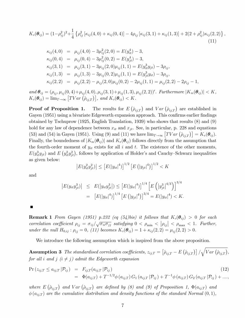
Kv(�ij) = (1��2ij)2+1

4

��2ij [�ij(4; 0) + �ij(0; 4)]� 4�ij [�ij(3; 1) + �ij(1; 3)] + 2(2 + �2ij)�ij(2; 2)

;

(11)

�ij(4; 0) = �ij(4; 0)� 3�2ij(2; 0) = E(y4it)� 3;�ij(0; 4) = �ij(0; 4)� 3�2ij(0; 2) = E(y4jt)� 3;�ij(3; 1) = �ij(3; 1)� 3�ij(2; 0)�ij(1; 1) = E(y3ityjt)� 3�ij;�ij(1; 3) = �ij(1; 3)� 3�ij(0; 2)�ij(1; 1) = E(y3jtyit)� 3�ij;�ij(2; 2) = �ij(2; 2)� �ij(2; 0)�ij(0; 2)� 2�ij(1; 1) = �ij(2; 2)� 2�ij � 1;

and �ij = (�ij; �ij(0; 4)+�ij(4; 0); �ij(3; 1)+�ij(1; 3); �ij(2; 2))0. Furthermore jKm(�ij)j < K,

Kv(�ij) = limT!1�TV ar

��ij;T

��, and Kv(�ij) < K.

Proof of Proposition 1. The results for E��ij;T

�and V ar

��ij;T

�are established in

Gayen (1951) using a bivariate Edgeworth expansion approach. This con�rms earlier �ndingsobtained by Tschuprow (1925, English Translation, 1939) who shows that results (8) and (9)hold for any law of dependence between xit and xjt. See, in particular, p. 228 and equations(53) and (54) in Gayen (1951). Using (9) and (11) we have limT!1

�TV ar

��ij;T

��= Kv(�ij).

Finally, the boundedness of jKm(�ij)j and Kv(�ij) follows directly from the assumption thatthe fourth-order moment of yit exists for all i and t. The existence of the other moments,E(y3ityjt) and E

�y2ity

2jt

�, follows by application of Holder�s and Cauchy�Schwarz inequalities

as given below: ��E(y2ity2jt)�� E(jyitj4)�1=2 �E �jyjtj4��1=2 < K

and ��E(yity3jt)�� E(��yity3jt��) � �E(jyitj4)�1=4 hE ��y3jt��4=3�i3=4

=�E(jyitj4)

�1=4 �E�jyjtj4

��3=4= E(jyitj4) < K:

Remark 1 From Gayen (1951) p.232 (eq (54)bis) it follows that Kv(�ij) > 0 for eachcorrelation coe¢ cient �ij = �ij=

p�ii�jj satisfying 0 < �min <

��ij�� < �max < 1. Further,under the null H0;ij : �ij = 0, (11) becomes Kv(�ij) = 1 + �ij(2; 2) = �ij(2; 2) > 0.

We introduce the following assumption which is inspired from the above proposition.

Assumption 3 The standardised correlation coe¢ cients, zij;T =��ij;T � E

��ij;T

��=qV ar

��ij;T

�,

for all i and j (i 6= j) admit the Edgeworth expansion

Pr (zij;T � aij;T jPij ) = Fij;T (aij;T jPij ) (12)

= �(aij;T ) + T�1=2� (aij;T )G1 (aij;T jPij ) + T�1� (aij;T )G2 (aij;T jPij ) + ::::;

where E��ij;T

�and V ar

��ij;T

�are de�ned by (8) and (9) of Proposition 1, �(aij;T ) and

� (aij;T ) are the cumulative distribution and density functions of the standard Normal (0; 1),

7

respectively, and Gs (aij;T jPij ), s = 1; 2; ::: are polynomials in aij;T , whose coe¢ cients dependon the underlying bivariate distribution of the observations (xit,xjt for t = 1; 2; :::; T ) whichis denoted by Pij.

Remark 2 While Assumption C1 of Cai and Liu (2011) characterising the tail-property ofyit can be used, we opt to focus on the standardised correlation coe¢ cient, zij;T . This is aself-normalised process where E

��ij;T

�and V ar

��ij;T

�are given by (8) and (9) respectively.

Then, for a �nite T , all moments of zij;T exist and as T !1, zij;T !d z s N(0; 1). Hence,following the theorem of Sargan (1976) on p.423 the Edgeworth expansion is valid.

Given Assumptions 1-3, �rst we establish the rate of convergence of the MT estimatorunder the spectral (or operator) norm which implies convergence in eigenvalues and eigen-vectors (see El Karoui (2008), and Bickel and Levina (2008a)).

Theorem 1 (Convergence under the spectral norm) Denote the sample correlation coe¢ -cient of xit and xjt over t = 1; 2; :::; T by �ij;T (as de�ned in (7) of Proposition 1) and thepopulation correlation matrix by R = (�ij). Suppose that Assumptions 1-3 hold. Let f(N)be an increasing function of N , p a �nite constant (0 < p < 1), and suppose there exist �niteT0 and N0 such that for all T > T0 and N > N0,

1� p

2f(N)> 0

andln f(N)=T ! 0; as N and T !1:

Then so long as N=pT ! 0 we have

E eRMT �R

spec

= O

�mNpT

�; (13)

where mN is de�ned by (3), eRMT = (~�ij;T ) = �ij;T I��ij;T �� > T�1=2cp(N)

�; and cp(N) =

��1�1� p

2f(N)

�> 0:

Proof. See Appendix.Under the conditions of Theorem 1, and since by Assumptions 1 and 2, �min (R) � "0 > 0,

then the eigenvalues of eRMT are bounded away from zero with probability approaching 1,and we have �eRMT

��1�R�1

spec

=

�eRMT

��1 �R� eRMT

�R�1

spec

� �min

�eRMT

��1 R� eRMT

spec

�min (R)�1

= Op

�mNpT

�:

Also see Appendix A of Fan et al. (2013) and proof of lemma A.1 in Fan et al. (2011).Similarly, we establish the rate of convergence of the MT estimator under the Frobenius

norm.

8

Theorem 2 (Convergence under the Frobenius norm) Denote the sample correlation coe¢ -cient of xit and xjt over t = 1; 2; :::; T by �ij;T (as de�ned in (7) of Proposition 1) and thepopulation correlation matrix by R = (�ij). Suppose that Assumptions 1-3 hold. Let f(N)be an increasing function of N , p a �nite constant (0 < p < 1), and suppose there exist �niteT0 and N0 such that for all T > T0 and N > N0,

1� p

2f(N)> 0;

ln f(N)=T ! 0; as N and T !1;

and

�max � limN!1ln [f(N)]

ln(N); (14)

where �max = supij [�ij], �ij =��ij(2; 2)

��ij = 0�, with �ij(2; 2) de�ned in Assumption 2.Then as long as N=

pT ! 0 we have

E eRMT �R

F= O

rmNN

T

!; (15)

where mN is de�ned by (3), eRMT = (~�ij;T ) = �ij;T I��ij;T �� > T�1=2cp(N)

�; and cp(N) =

��1�1� p

2f(N)

�> 0:

Proof. See Appendix.

Remark 3 For the convergence of the Frobenius norm, E eRMT �R

F, at the rate of

Op

�pmNN=T

�, the rate at which f(N) rises with N is dictated by the magnitude of �max.

For example if �max = 1; setting f(N) = N � 1 meets all the conditions of Theorem 2. Butfor values of �max > 1, we need f(N) to rise with N at a faster rate. For �max 2 (1; 2], it issu¢ cient to set f(N) = N(N � 1)=2. It is easily seen that in this case

limN!1

�ln f(N)

ln(N)� �max

�= lim

N!1

�ln(N) + ln(N � 1)� ln(2)

ln(N)� �max

�= 2� �max;

and the conditions are met if �max � 2. Similarly, for �max � 3 we need to specify f(N) =O(N3).

Remark 4 While in practice we �nd it reasonable to set �max no greater than two, furtherresearch is required in determining this data dependent measure, which is beyond the scopeof the present paper. Convergence under the spectral norm is less demanding than under theFrobenius norm. Unlike Theorem 2, the statement of Theorem 1 does not require a conditionon �max. This implies that under the spectral norm, when controlling the errors in estimationof R; it is su¢ cient for f(N) to rise linearly with N irrespective of the value of �max.

9

Remark 5 The orders of convergence in (13) and (15) are in line with the results in thethresholding literature. See, for example, Theorem 1 of Cai and Liu (2011, CL), and Bickeland Levina (2008b, BL), with q = 0, that state the convergence rate using the spectral norm

in terms of probability, e��

spec= Op

�mN

qlog(N)T

�, where e� is the thresholded es-

timator of � using either the CL or BL approaches. Similarly, Theorem 2 of Bickel andLevina (2008b), with q = 0, using the Frobenius norm under the Gaussianity assumption,

obtains a convergence rate of e��

F= Op

�qmNN log(N)

T

�. In fact (13) and (15) are

improvements on the existing rates since the log (N) factor is absent in both cases. The rateof Op

�pmNT

�is achieved in the shrinkage literature as well if the assumption of sparseness

is imposed. Here mN also can be assumed to rise with N in which case the rate of conver-gence becomes slower. This compares with a rate of Op

�pN=T

�for the sample covariance

(correlation) matrix - see Theorem 3.1 in Ledoit and Wolf (2004 - LW). Note that LW usean unconventional de�nition for the Frobenius norm (see their De�nition 1 p. 376).

Remark 6 Results (13) and (15) also hold if a concept of �approximate�sparseness is used inplace of Assumption 1, such that mN is de�ned more generally as mN = maxi�N

PNj=1 j�ijj

q,for some q 2 [0; 1). See Bickel and Levina (2008b) or Fan et al. (2013).

Remark 7 It is interesting to note that application of the Bonferroni procedure to the prob-lem of testing �ij = 0 for all i 6= j, is equivalent to setting f(N) = N(N � 1)=2: Ourtheoretical results suggest that this is too conservative if �ij = 0 implies xit and xjt areindependent, but could be appropriate otherwise. In our Monte Carlo study we consider ob-servations with linear and non-linear dependence, and experiment with f(N) = N � 1 andf(N) = N(N � 1)=2: We �nd that the simulation results conform closely to our theoretical�ndings.

Consider now the issue of consistent support recovery of R (or �), which is de�ned interms of true positive rate (TPR) and false positive rate (FPR) statistics. Consistent supportrecovery requires TPR ! 1 and FPR ! 0 with probability 1 as N and T ! 1, and doesnot follow from the results obtained above on the convergence rates of di¤erent estimatorsof R. The problem is addressed in the following theorem.

Theorem 3 (Support Recovery) Consider the true positive rate (TPR) and the false positiverate (FPR) statistics computed using the multiple testing estimator

~�ij;T = �ij;T I��ij;T �� > T�1=2cp(N)

�;

10

given by

TPR =

PPi6=j

I(~�ij;T 6= 0; and �ij 6= 0)PPi6=j

I(�ij 6= 0)(16)

FPR =

PPi6=j

I(~�ij;T 6= 0; and �ij = 0)PPi6=j

I(�ij = 0); (17)

where �ij;T is the pair-wise correlation coe¢ cient de�ned by (7), cp(N) = ��1�1� p

2f(N)

�>

0, 0 < p < 1, f(N) is an increasing function such that cp(N) ! 1, as N ! 1,ln f(N)=T ! 0 and cp(N)=

pT ! 0, as N and T ! 1. Suppose also that Assumptions

1-3 hold. Then with probability tending to 1, TPR = 1, and with probability tending to 1,FPR = 0, if there exist N0 and T0 such that for N > N0 and T > T0,

pT�min �cp(N) > 0,

where �min = minij��ij�� > 0.

Proof. See Appendix.

Remark 8 The proof of support recovery does not depend on �ij(2; 2). Also it only requiresthat f(N) rises with N linearly. For example, setting f(N) = N � 1 it is easily seen thatln f(N)=T = ln(N � 1)=T ! 0; as N and T ! 1, and cp(N) = ��1

�1� p

2f(N)

�! 1, as

N ! 1, and conditions of Theorem 3 are met. Interestingly, this suggests that consistentsupport recovery is ensured if Bonferroni�s MT procedure is applied to R (or �) row-wise.One is likely to encounter loss of power if Bonferroni�s procedure is applied to all the distincto¤-diagonal elements of R. A similar argument can be made for Holm�s MT procedure,although the application of Holm�s procedure row-wise can result in contradictions due to thesymmetry of the correlation matrix.

3 Monte Carlo simulations

We investigate the numerical properties of the proposed multiple testing (MT ) estimatorusing Monte Carlo simulations. We compare our estimator with a number of thresholdingand shrinkage estimators proposed in the literature, namely the thresholding estimators ofBickel and Levina (2008b, BL) and Cai and Liu (2011, CL), and the shrinkage estimator ofLW. As mentioned earlier the thresholding methods of BL and CL require the computationof a theoretical constant, C, that arises in the rate of their convergence. For this purpose,cross-validation is typically employed which we use when implementing these estimators. Forthe CL approach we also consider the theoretical value of C = 2 proposed by the authors.A review of these estimators along with details of the associated cross-validation procedurecan be found in the Supplementary Appendix B.We begin by generating the standardised variates, yit, as

yt = Put; t = 1; 2; :::; T;

11

where yt = (y1t; y2t; :::; yNt)0, ut = (u1t; u2t; :::; uNt)0, and P is the Cholesky factor associatedwith the choice of the correlation matrix R = PP 0. We consider two alternatives for theerrors, uit: (i) the benchmark Gaussian case where uit s IIDN(0; 1) for all i and t, and (ii)the case where uit follows a multivariate t-distribution with v degrees of freedom generatedas

uit =

�v� 2�2v;t

�1=2"it, for i = 1; 2; :::; N;

where "it s IIDN(0; 1), and �2v;t is a chi-squared random variate with v > 4 degrees offreedom, distributed independently of "it for all i and t. As fourth-order moments are requiredby Assumption 2 we set v = 8 to ensure that E (y4it) exists and �max � 2. Note that under�ij = 0; �ij = �ij(2; 2

��ij = 0) = (v�2)=(v�4), and with v = 8 we have �ij = �� = 1:5.Therefore, in the case where the standardised errors are multivariate t-distributed to ensurethat conditions of Theorem 2 are met we must set f(N) = N (N � 1) =2. (See also Remark3 and Lemma 7 in the Supplementary Appendix A). One could further allow for fat-tailed"it shocks, though fat-tail shocks alone (e.g. generating uit as such) do not necessarily resultin �ij > 1 as shown in Lemma 8 of the Supplementary Appendix A. The same is true fornormal shocks under case (i), where �ij(2; 2) = 1 whether P = IN or not. In such casessetting f(N) = N � 1 is then su¢ cient for conditions of Theorem 2 to be met.Next, the non-standardised variates xt = (x1t;x2t; :::;xNt)

0 are generated as

xt = a+ ft +D1=2yt, (18)

where D = diag(�11; �22; ::::; �NN), a = (a1; a2; :::; aN)0 and = ( 1; 2; :::; N)0.

We report results for N = f30; 100; 200g and T = 100; for the baseline case where = 0 and a = 0 in (18). The properties of the MT procedure when factors are includedin the data generating process are also investigated by drawing i and ai as IIDN (1; 1) fori = 1; 2; ::::; N , and generating ft, the common factor, as a stationary AR(1) process, but tosave space these results are made available upon request. Under both settings we focus onthe residuals from an OLS regression of xt on an intercept and a factor (if needed).In accordance with our theoretical assumptions we consider two exactly sparse covariance

(correlation) matrices:Monte Carlo design A: Following Cai and Liu (2011) we consider the banded matrix

� = (�ij) = diag(A1;A2);

whereA1 = A+�IN=2,A = (aij)1�i;j�N=2; aij = (1� ji�jj10)+ with � = max(��min(A); 0)+0:01

to ensure that A is positive de�nite, and A2 = 4IN=2: � is a two-block diagonal matrix,A1 is a banded and sparse covariance matrix, and A2 is a diagonal matrix with 4 along thediagonal. Matrix P is obtained numerically by applying the Cholesky decomposition to thecorrelation matrix, R = D�1=2�D�1=2 = PP0, where the diagonal elements of D are givenby �ii = 1 + �; for i = 1; 2; :::; N=2 and �ii = 4; for i = N=2 + 1; N=2 + 1; :::; N:

Monte Carlo design B : We consider a covariance structure that explicitly controls for thenumber of non-zero elements of the population correlation matrix. First we draw the N � 1

12

vector b = (b1; b2; :::; bN)0 with elements generated as Uniform (0:7; 0:9) for the �rst and

last Nb (< N) elements of b, where Nb =�N ��, and set the remaining middle elements of b

to zero. The resulting population correlation matrix R is de�ned by

R = IN + bb0 � diag (bb0) , (19)

for whichpT�min �cp(N) > 0 and �min = minij

��ij�� > 0, in line with Theorem 3. Thedegree of sparseness of R is determined by the value of the parameter �. We are interestedin weak cross-sectional dependence, so we focus on the case where � < 1=2 following Pesaran(2015), and set � = 0:25. Matrix P is then obtained by applying the Cholesky decompositionto R de�ned by (19). Further, we set � = D1=2RD1=2, where the diagonal elements of Dare given by �ii s IID (1=2 + �2(2)=4), i = 1; 2; :::; N .An additional two covariance speci�cations based on approximately sparse matrices as

de�ned in Bickel and Levina (2008b, p. 2580 for 0 < q < 1), namely the correlation matricescorresponding to an AR(1) and spatial AR(1), SAR(1), process respectively, along with theirassociated simulation results can be found in the Supplementary Appendix D.

3.1 Finite sample positive de�niteness

As with other thresholding approaches, multiple testing preserves the symmetry of R and isinvariant to the ordering of the variables but it does not ensure positive de�niteness of theestimated covariance matrix when N > T .A number of methods have been developed in the literature that produce sparse inverse

covariance matrix estimates which make use of a penalised likelihood (D�Aspremont et al.(2008), Rothman et al. (2008, 2009), Yuan and Lin (2007), and Peng et al. (2009)) orconvex optimisation techniques that apply suitable penalties such as a logarithmic barrierterm (Rothman (2012)), a positive de�niteness constraint (Xue et al. (2012)), an eigenvaluecondition (Liu et al. (2013), Fryzlewicz (2013), Fan et al. (2013, FLM)). Most of theseapproaches are rather complex and computationally extensive.A simpler alternative, which conceptually relates to soft thresholding (such as smoothly

clipped absolute deviation by Fan and Li (2001) and adaptive lasso by Zou (2006)), is toconsider a convex linear combination of eRMT and a well-de�ned target matrix which isknown to result in a positive de�nite matrix. In what follows, we opt to set as benchmarktarget the N�N identity matrix, IN , in line with one of the methods suggested by El Karoui(2008). The advantage of doing so lies in the fact that the same support recovery achievedby eRMT is maintained and the diagonal elements of the resulting correlation matrix do notdeviate from unity. Given the similarity of this adjustment to the shrinking method, we dubthis step shrinkage on our multiple testing estimator (S-MT ),

eRS-MT (�) = �IN + (1� �)eRMT ; (20)

with shrinkage parameter � 2 (�0; 1]; and �0 being the minimum value of � that produces anon-singular eRS-MT (�0) matrix. Alternative ways of computing the optimal weights on the

13

two matrices can be entertained. We choose to calibrate, �, since opting to use �0 in (20),as suggested in El Karoui (2008), does not necessarily provide a well-conditioned estimateof eRS-MT . Accordingly, we set � by solving the following optimisation problem

�� = arg min�0+��1

R�10 �eR�1

S-MT (�) 2F; (21)

where � is a small positive constant, and R0 is a reference invertible correlation matrix.Finally, we construct the corresponding covariance matrix as

e�S-MT (��) = D

1=2 eRS-MT (��) D

1=2:

Further details on the S-MT procedure, the optimisation of (21) and choice of referencematrix R0 are available in the Supplementary Appendix C.

3.2 Alternative estimators and evaluation metrics

Using the earlier set up and the relevant adjustments to achieve positive de�niteness of theestimators of � where required, we obtain the following estimates of �:

MTN�1: thresholding based on theMT approach applied to the sample correlation matrix(e�MT ) using f(N) = N � 1 (e�MTN�1)

MTN(N�1)=2: thresholding based on the MT approach applied to the sample correlationmatrix (e�MT ) using f(N) = N(N � 1)=2 (e�MTN(N�1)=2)

BLC : BL thresholding on the sample covariance matrix using cross-validated C (e�BL;C)CL2: CL thresholding on the sample covariance matrix using the theoretical value of

C = 2 (e�CL;2)CLC : CL thresholding on the sample covariance matrix using cross-validated C (e�CL;C)

S-MTN�1: supplementary shrinkage applied to MTN�1 (e�S-MTN�1)S-MTN(N�1)=2: supplementary shrinkage applied to MTN(N�1)=2 (e�S-MTN(N�1)=2)BLC�: BL thresholding using the Fan, Liao and Mincheva (2013, FLM) cross-validation

adjustment procedure for estimating C to ensure positive de�niteness (e�BL;C�)CLC�: CL thresholding using the FLM cross-validation adjustment procedure for esti-

mating C to ensure positive de�niteness (e�CL;C�)

LW�: LW shrinkage on the sample covariance matrix (�LW�).

In accordance with the theoretical results in Theorem 2 and in view of Remark 3, we con-sider two versions of theMT estimator depending on the choice of f(N) = fN � 1; N(N � 1)=2g :The BLC , and CL2 and CLC estimators apply the thresholding procedure without ensuringthat the resultant covariance estimators are invertible. The next �ve estimators yield in-vertible covariance estimators. The S-MT estimators are obtained using the supplementaryshrinkage approach described in Section 3.1. BLC� and CLC� estimators are obtained byapplying the additional FLM adjustments. The shrinkage estimator, LW�, is invertible byconstruction. In the case of the MT estimators where regularisation is performed on thecorrelation matrix the associated covariance matrix is estimated as D1=2 eRMT D

1=2.

14

For both Monte Carlo designs A and B, we compute the spectral and Frobenius norms ofthe deviations of each of the regularised covariance matrices from their respective population� : ��

specand

�� F; (22)

where �� is set to one of the following estimators fe�MTN�1 ;e�MTN(N�1)=2 ;

e�BL;C ;e�CL;2;e�CL;C ;

e�S-MTN�1 ;e�S-MTN(N�1)=2 ;

e�BL;C� ;e�CL;C� ; �LW�

g. The threshold values, C and

C�, are obtained by cross-validation (see Supplementary Appendix B.3 for details). Bothnorms are also computed for the di¤erence between ��1, the population inverse of �, andthe estimators fe��1

S-MTN�1; e��1S-MTN(N�1)=2

; e��1BL;C� ;

e��1CL;C� ; ��1LW�

g. Further, we investigate theability of the thresholding estimators to recover the support of the true covariance matrixvia the true positive rate (TPR) and false positive rate (FPR), as de�ned by (16) and (17),respectively. The statistics TPR and FPR are not relevant to the shrinkage estimator LW�

and will not be reported for this estimator.

3.3 Robustness of MT to the choice of the p-value and f(N)

We begin by investigating the sensitivity of theMT estimator to the choice of the p-value, p,and the scaling factor f(N) used in the formulation of cp(N) de�ned by (6). For this purposewe consider the typical signi�cance levels used in the literature, namely p = f0:01; 0:05; 0:10g;and f(N) = fN � 1; N(N � 1)=2g. Table 1 summarises the spectral and Frobenius normlosses (averaged over 2000 replications) for both Monte Carlo designs A and B, and forboth distributional error assumptions (Gaussian and multivariate t). First, we note thatneither of the norms is much a¤ected by the choice of the p values when the scaling factoris N (N � 1) =2, irrespective of whether the observations are drawn from a Gaussian or amultivariate t distribution. Perhaps this is to be expected since for N su¢ ciently large thee¤ective p-value which is given by 2p=N(N�1) is very small and the test outcomes are morelikely to be robust to the changes in the values of p as compared to the case when the scalingfactor used is N � 1. The results in Table 1 also con�rm our theoretical �nding of Theorem2 that in the case of Gaussian observations, where �max = 1, the scaling factor N�1 is likelyto perform better as compared to N(N � 1)=2, but the reverse is true if the observationsare multivariate t distributed and the scaling factor N(N � 1)=2 is to be preferred (see alsoRemark 3). We also note that all the norm losses rise with N given that T is kept at 100 inall the experiments. We obtain similar results when we consider other Monte Carlo designswith approximately sparse covariance matrices. To save space the results for these designsare provided in the Supplementary Appendix D. Overall, we �nd that the results are morerobust when the scaling factor N(N � 1)=2 is used.

3.4 Norm comparisons of MT , BL, CL, and LW estimators

In comparing our proposed estimators with those in the literature we consider a fewer num-ber of Monte Carlo replications and report the results with norm losses averaged over 100

15

replications, given the use of the cross-validation procedure in the implementation of BL andCL thresholding. This Monte Carlo speci�cation is in line with the simulation set up of BLand CL. Our reported results are also in agreement with their �ndings.Tables 2 and 3 summarise the results for the Monte Carlo designs A and B, respectively.

Based on the results of Section 3.3, we provide norm comparisons for the MT estimatorusing the scaling factor N(N � 1)=2; and the conventional signi�cance level of p = 0:05.Initially, we consider the threshold estimators, MT , BL and the two versions of the CLestimators (CL2 and CLC) without further adjustments to ensure invertibility. First, wenote that the MT and CL estimators (both versions) dominate the BL estimator in everycase, without any exceptions and for both designs. The same is also true if we compareMT and CL estimators to the LW shrinkage estimator, although it could be argued that itis more relevant to compare the invertible versions of the MT and CL estimators (namelye�CL;C� and e�S-MT ) with �LW�

. In such comparisons �LW�performs relatively better,

nevertheless, �LW�is still dominated by e�S-MT , with a few exceptions in the case of design

A and primarily when N = 30. However, no clear ordering emerges when we compare �LW�

with e�CL;C�.

3.5 Norm comparisons of inverse estimators

Although the theoretical focus of this paper has been on estimation of � rather than itsinverse, it is still of interest to see how well e��1

S-MT , e��1BL;C�, e��1CL;C�, and �

�1LW�

estimate��1, assuming that ��1 is well de�ned. Table 4 provides average norm losses for MonteCarlo design B whose � is positive de�nite. � for design A is ill-conditioned and willnot be considered any further here. As can be seen from the results in Table 4, e��1S-MT

performs much better than e��1BL;C� and e��1CL;C� for Gaussian and multivariate t-distributed

observations. In fact, the average spectral norms for e��1BL;C� and e��1CL;C� include some sizeableoutliers, especially for N � 100. However, the ranking of the di¤erent estimators remains thesame if we use the Frobenius norm which appears to be less sensitive to the outliers. It is alsoworth noting that e��1

S-MT performs better than LW�, for all sample sizes and irrespective ofwhether the observations are drawn as Gaussian or multivariate t.

3.6 Support recovery statistics

Table 5 reports the true positive and false positive rates (TPR and FPR) for the supportrecovery of � using the multiple testing and thresholding estimators. In the comparison setwe include two versions of the MT estimator (e�MTN�1 and e�MTN(N�1)=2); e�BL;C ;

e�CL;2; ande�CL;C . Again we use 100 replications due to the use of cross-validation in the implementationof BL and CL thresholding. We include the MT estimators for both choices of the scalingfactor, f(N) = N�1 and f(N) = N(N�1)=2, computed at p = 0:05, to see if our theoreticalresult, namely that for consistent support recovery only the linear scaling factor, N � 1, isneeded, is borne out by the simulations. For consistent support recovery we would like to see

16

FPR values near zero and TPR values near unity. As can be seen from Table 5, the FPRvalues of all estimators are very close to zero, so any comparisons of di¤erent estimatorsmust be based on the TPR values. Comparing the results for e�MTN�1 and e�MTN(N�1)=2 we

�nd that as predicted by the theory (Theorem 3 and Remark 8), TPR values of e�MTN�1 arecloser to unity as compared to the TPR values of e�MTN(N�1)=2 . Similar results are obtainedfor the MT estimators for di¤erent choices of the p values. Table 6 provides results forp = f0:01; 0:05; 0:10g; and for f(N) = fN � 1; N(N � 1)=2g using 2,000 replications. Inthis table it is further evident that, in line with the conclusions of Section 3.3, both theTPR and the FPR statistics are relatively robust to the choice of the p values irrespectiveof the scaling factor, f(N), or whether the observations are drawn from a Gaussian or amultivariate t distribution. This is especially true under design B, since for this speci�cationwe explicitly control for the number of non-zero elements in �, that ensures the conditionsof Theorem 3 are met.Turning to a comparison with other estimators in Table 5, we �nd that the MT and

CL estimators perform substantially better than the BL estimator. Further, allowing fornon-linear dependence in the errors causes the support recovery performance of BLC ; CL2and CLC to deteriorate noticeably whileMTN�1 andMTN(N�1)=2 remain remarkably stable.Finally, again note that TPR values are higher for design B. Overall, the estimator e�MTN�1

does best in recovering the support of� as compared to other estimators, although the resultsof CL and MT for support recovery are very close, which is in line with the comparativeanalysis carried out in terms of the relative norm losses of these estimators.

3.7 Computational demands of the di¤erent thresholding methods

Table 7 reports the relative execution times of the di¤erent thresholding methods studied.All times are relative to the time it takes to carry out the computations for the MTN(N�1)=2estimator. It took 0:010, 0:013, and 0:016 seconds to apply the MT method in Matlab toa sample of N = f30; 100; 200g; respectively, and T = 100 observations using a desktoppc. The slight di¤erence in execution time between MTN�1 and MTN(N�1)=2 amounts tothe stricter condition imposed by the p-value on the MTN(N�1)=2 procedure, which producesa slightly sparser version of e�. In contrast, the BLC and CLC thresholding approachesare computationally much more demanding. Their computations took between about 18and 412293 times longer than the MT approach, for the same sample sizes and computerhardware. The BLC method was less demanding than the CLC method - it took betweenabout 18 and 500 times longer than the MT approach. Even CL2, which does not requireestimation of the threshold parameter, took up to 17 times longer than the MT approach.Thus, compared with other thresholding methodsMT has a clear computational advantage.

4 Concluding Remarks

This paper considers regularisation of large covariance matrices particularly when the crosssection dimension N of the data under consideration exceeds the time dimension T: In this

17

case the sample covariance matrix, �; becomes ill-conditioned and is not a satisfactoryestimator of the population covariance.A regularisation estimator is proposed which uses multiple testing rather than cross-

validation to calibrate the threshold value. It is shown that the resultant estimator has aconvergence rate of

�mNT

�1=2� under the spectral norm and (mNN=T )1=2 under the Frobe-

nius norm, where T is the number of observations, and mN is bounded in N (the dimensionof �), which provide slightly better rates than the convergence rates established in the lit-erature for other regularised covariance matrix estimators. Our results derived under theFrobenius norm explicitly relate the scaling function in the multiple testing problem to thepossible non-linear dependence of the underlying data, and together with the spectral normresults are valid under both Gaussian and non-Gaussian assumptions. This complimentsthe existing theoretical results in the literature for the Frobenius norm of the thresholdingestimator derived only under the assumption of Gaussianity. As compared to the thresholdestimators that use cross-validation, the MT estimator is also computationally simple andfast to implement.The numerical properties of the proposed estimator are investigated using Monte Carlo

simulations. It is shown that the MT estimator performs well, and generally better thanthe other estimators proposed in the literature. The simulations also show that in terms ofspectral and Frobenius norm losses, the MT estimator is reasonably robust to the choice ofp in the threshold criterion,

��ij�� > T�1=2��1�1� p

2f(N)

�, particularly when f(N) is set to

N(N � 1)=2. For support recovery, better results are obtained if f(N) is set to N � 1.

18

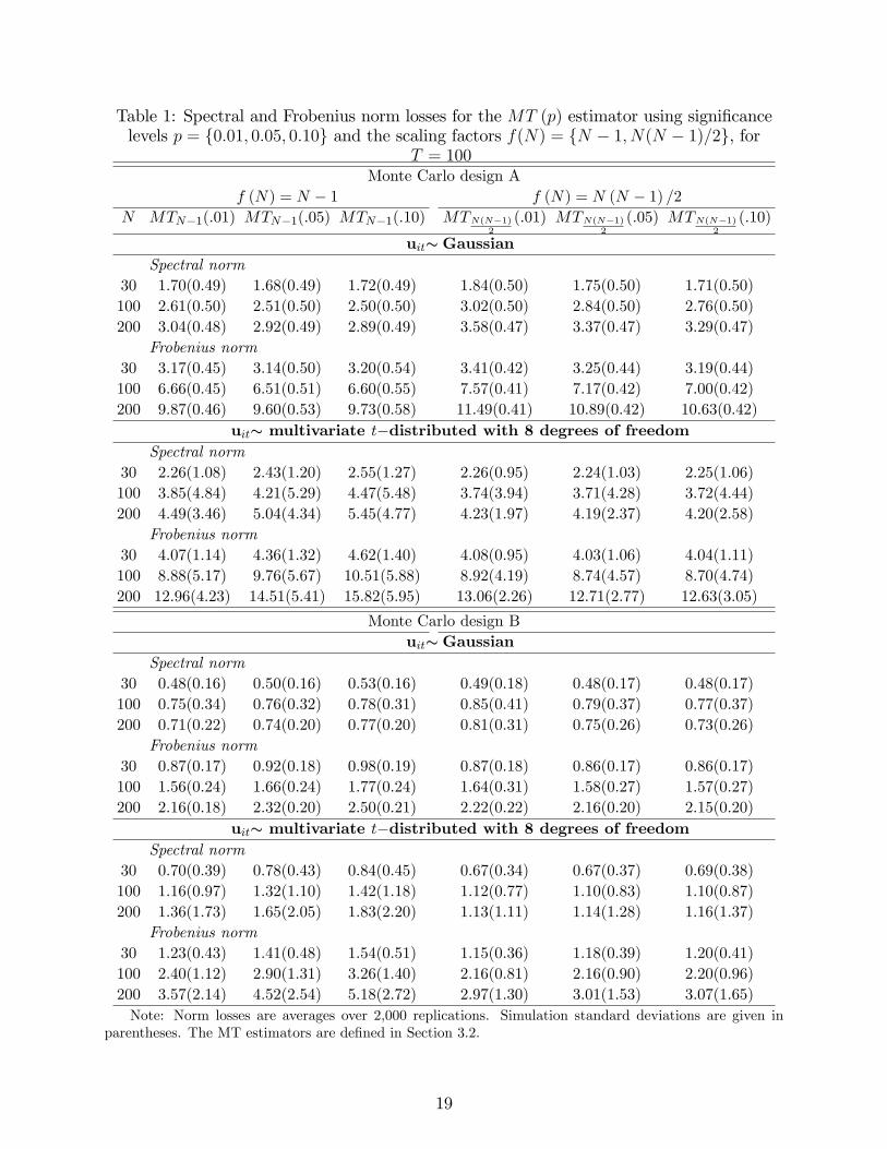
Table 1: Spectral and Frobenius norm losses for the MT (p) estimator using signi�cancelevels p = f0:01; 0:05; 0:10g and the scaling factors f(N) = fN � 1; N(N � 1)=2g, for

T = 100Monte Carlo design A

f (N) = N � 1 f (N) = N (N � 1) =2N MTN�1(:01) MTN�1(:05) MTN�1(:10) MTN(N�1)

2

(:01) MTN(N�1)2

(:05) MTN(N�1)2

(:10)

uits GaussianSpectral norm

30 1.70(0.49) 1.68(0.49) 1.72(0.49) 1.84(0.50) 1.75(0.50) 1.71(0.50)100 2.61(0.50) 2.51(0.50) 2.50(0.50) 3.02(0.50) 2.84(0.50) 2.76(0.50)200 3.04(0.48) 2.92(0.49) 2.89(0.49) 3.58(0.47) 3.37(0.47) 3.29(0.47)

Frobenius norm30 3.17(0.45) 3.14(0.50) 3.20(0.54) 3.41(0.42) 3.25(0.44) 3.19(0.44)100 6.66(0.45) 6.51(0.51) 6.60(0.55) 7.57(0.41) 7.17(0.42) 7.00(0.42)200 9.87(0.46) 9.60(0.53) 9.73(0.58) 11.49(0.41) 10.89(0.42) 10.63(0.42)

uits multivariate t�distributed with 8 degrees of freedomSpectral norm

30 2.26(1.08) 2.43(1.20) 2.55(1.27) 2.26(0.95) 2.24(1.03) 2.25(1.06)100 3.85(4.84) 4.21(5.29) 4.47(5.48) 3.74(3.94) 3.71(4.28) 3.72(4.44)200 4.49(3.46) 5.04(4.34) 5.45(4.77) 4.23(1.97) 4.19(2.37) 4.20(2.58)

Frobenius norm30 4.07(1.14) 4.36(1.32) 4.62(1.40) 4.08(0.95) 4.03(1.06) 4.04(1.11)100 8.88(5.17) 9.76(5.67) 10.51(5.88) 8.92(4.19) 8.74(4.57) 8.70(4.74)200 12.96(4.23) 14.51(5.41) 15.82(5.95) 13.06(2.26) 12.71(2.77) 12.63(3.05)

Monte Carlo design Buits Gaussian

Spectral norm30 0.48(0.16) 0.50(0.16) 0.53(0.16) 0.49(0.18) 0.48(0.17) 0.48(0.17)100 0.75(0.34) 0.76(0.32) 0.78(0.31) 0.85(0.41) 0.79(0.37) 0.77(0.37)200 0.71(0.22) 0.74(0.20) 0.77(0.20) 0.81(0.31) 0.75(0.26) 0.73(0.26)

Frobenius norm30 0.87(0.17) 0.92(0.18) 0.98(0.19) 0.87(0.18) 0.86(0.17) 0.86(0.17)100 1.56(0.24) 1.66(0.24) 1.77(0.24) 1.64(0.31) 1.58(0.27) 1.57(0.27)200 2.16(0.18) 2.32(0.20) 2.50(0.21) 2.22(0.22) 2.16(0.20) 2.15(0.20)

uits multivariate t�distributed with 8 degrees of freedomSpectral norm

30 0.70(0.39) 0.78(0.43) 0.84(0.45) 0.67(0.34) 0.67(0.37) 0.69(0.38)100 1.16(0.97) 1.32(1.10) 1.42(1.18) 1.12(0.77) 1.10(0.83) 1.10(0.87)200 1.36(1.73) 1.65(2.05) 1.83(2.20) 1.13(1.11) 1.14(1.28) 1.16(1.37)

Frobenius norm30 1.23(0.43) 1.41(0.48) 1.54(0.51) 1.15(0.36) 1.18(0.39) 1.20(0.41)100 2.40(1.12) 2.90(1.31) 3.26(1.40) 2.16(0.81) 2.16(0.90) 2.20(0.96)200 3.57(2.14) 4.52(2.54) 5.18(2.72) 2.97(1.30) 3.01(1.53) 3.07(1.65)Note: Norm losses are averages over 2,000 replications. Simulation standard deviations are given in

parentheses. The MT estimators are de�ned in Section 3.2.

19

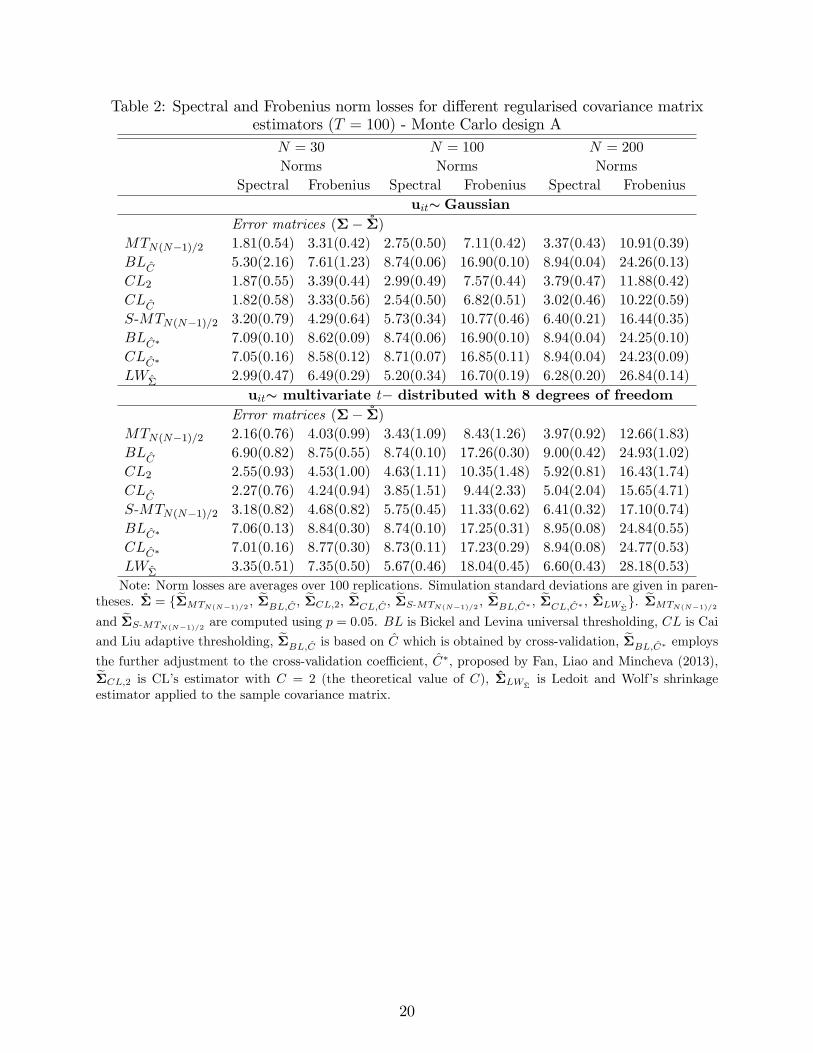
Table 2: Spectral and Frobenius norm losses for di¤erent regularised covariance matrixestimators (T = 100) - Monte Carlo design A

N = 30 N = 100 N = 200

Norms Norms NormsSpectral Frobenius Spectral Frobenius Spectral Frobenius

uits GaussianError matrices (��)

MTN(N�1)=2 1.81(0.54) 3.31(0.42) 2.75(0.50) 7.11(0.42) 3.37(0.43) 10.91(0.39)BLC 5.30(2.16) 7.61(1.23) 8.74(0.06) 16.90(0.10) 8.94(0.04) 24.26(0.13)CL2 1.87(0.55) 3.39(0.44) 2.99(0.49) 7.57(0.44) 3.79(0.47) 11.88(0.42)CLC 1.82(0.58) 3.33(0.56) 2.54(0.50) 6.82(0.51) 3.02(0.46) 10.22(0.59)S-MTN(N�1)=2 3.20(0.79) 4.29(0.64) 5.73(0.34) 10.77(0.46) 6.40(0.21) 16.44(0.35)BLC� 7.09(0.10) 8.62(0.09) 8.74(0.06) 16.90(0.10) 8.94(0.04) 24.25(0.10)CLC� 7.05(0.16) 8.58(0.12) 8.71(0.07) 16.85(0.11) 8.94(0.04) 24.23(0.09)LW� 2.99(0.47) 6.49(0.29) 5.20(0.34) 16.70(0.19) 6.28(0.20) 26.84(0.14)

uits multivariate t� distributed with 8 degrees of freedomError matrices (��)

MTN(N�1)=2 2.16(0.76) 4.03(0.99) 3.43(1.09) 8.43(1.26) 3.97(0.92) 12.66(1.83)BLC 6.90(0.82) 8.75(0.55) 8.74(0.10) 17.26(0.30) 9.00(0.42) 24.93(1.02)CL2 2.55(0.93) 4.53(1.00) 4.63(1.11) 10.35(1.48) 5.92(0.81) 16.43(1.74)CLC 2.27(0.76) 4.24(0.94) 3.85(1.51) 9.44(2.33) 5.04(2.04) 15.65(4.71)S-MTN(N�1)=2 3.18(0.82) 4.68(0.82) 5.75(0.45) 11.33(0.62) 6.41(0.32) 17.10(0.74)BLC� 7.06(0.13) 8.84(0.30) 8.74(0.10) 17.25(0.31) 8.95(0.08) 24.84(0.55)CLC� 7.01(0.16) 8.77(0.30) 8.73(0.11) 17.23(0.29) 8.94(0.08) 24.77(0.53)LW� 3.35(0.51) 7.35(0.50) 5.67(0.46) 18.04(0.45) 6.60(0.43) 28.18(0.53)Note: Norm losses are averages over 100 replications. Simulation standard deviations are given in paren-

theses. �� = fe�MTN(N�1)=2 ;e�BL;C ; e�CL;2; e�CL;C ; e�S-MTN(N�1)=2 ;

e�BL;C� ; e�CL;C� ; �LW�g. e�MTN(N�1)=2

and e�S-MTN(N�1)=2 are computed using p = 0:05. BL is Bickel and Levina universal thresholding, CL is Cai

and Liu adaptive thresholding, e�BL;C is based on C which is obtained by cross-validation, e�BL;C� employs

the further adjustment to the cross-validation coe¢ cient, C�, proposed by Fan, Liao and Mincheva (2013),e�CL;2 is CL�s estimator with C = 2 (the theoretical value of C), �LW�is Ledoit and Wolf�s shrinkage

estimator applied to the sample covariance matrix.

20

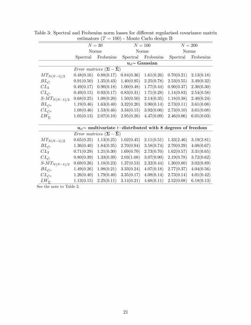
Table 3: Spectral and Frobenius norm losses for di¤erent regularised covariance matrixestimators (T = 100) - Monte Carlo design B

N = 30 N = 100 N = 200


uits GaussianError matrices (��)


uits multivariate t�distributed with 8 degrees of freedomError matrices (��)


See the note to Table 2.

21

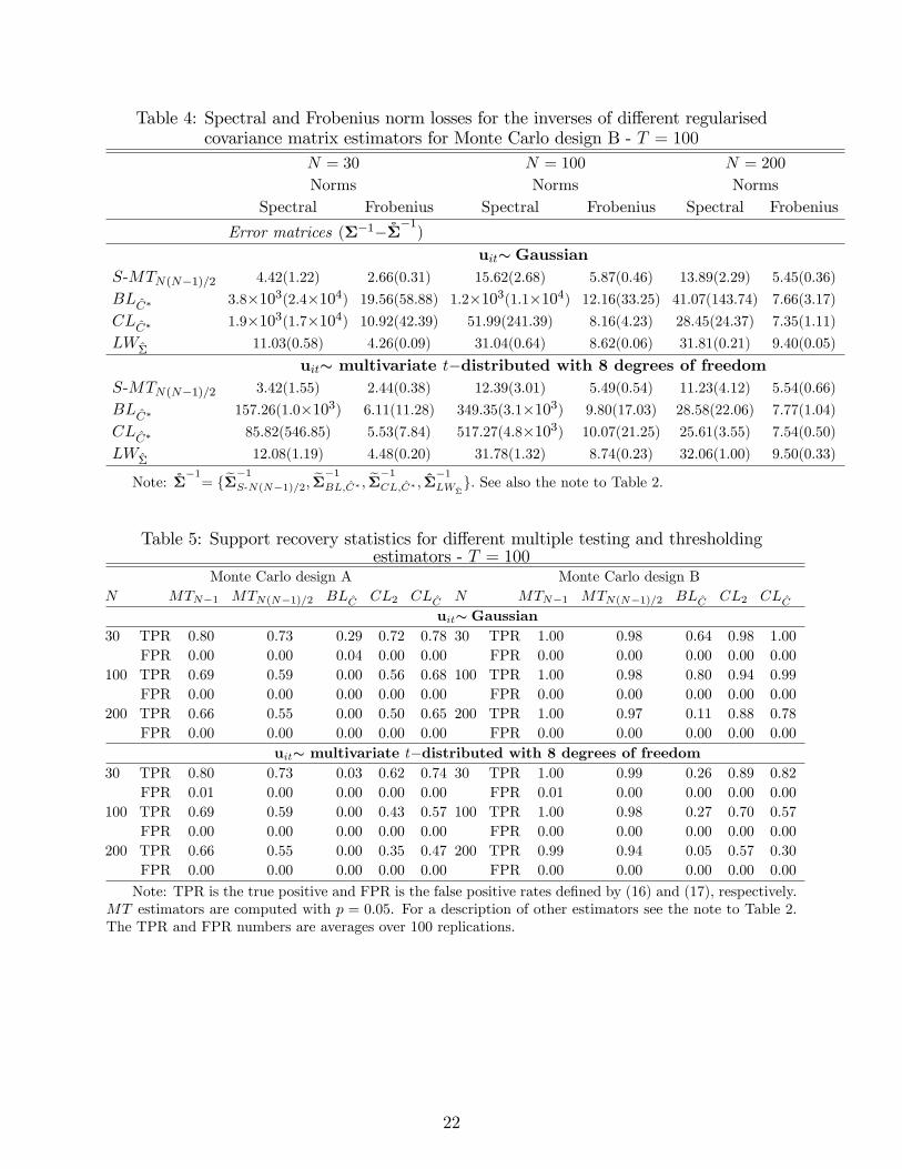
Table 4: Spectral and Frobenius norm losses for the inverses of di¤erent regularisedcovariance matrix estimators for Monte Carlo design B - T = 100

N = 30 N = 100 N = 200


Error matrices (��1��1)uits Gaussian

S-MTN(N�1)=2 4.42(1.22) 2.66(0.31) 15.62(2.68) 5.87(0.46) 13.89(2.29) 5.45(0.36)

BLC� 3.8�103(2.4�104) 19.56(58.88) 1.2�103(1.1�104) 12.16(33.25) 41.07(143.74) 7.66(3.17)

CLC� 1.9�103(1.7�104) 10.92(42.39) 51.99(241.39) 8.16(4.23) 28.45(24.37) 7.35(1.11)

LW� 11.03(0.58) 4.26(0.09) 31.04(0.64) 8.62(0.06) 31.81(0.21) 9.40(0.05)

uits multivariate t�distributed with 8 degrees of freedomS-MTN(N�1)=2 3.42(1.55) 2.44(0.38) 12.39(3.01) 5.49(0.54) 11.23(4.12) 5.54(0.66)

BLC� 157.26(1.0�103) 6.11(11.28) 349.35(3.1�103) 9.80(17.03) 28.58(22.06) 7.77(1.04)

CLC� 85.82(546.85) 5.53(7.84) 517.27(4.8�103) 10.07(21.25) 25.61(3.55) 7.54(0.50)

LW� 12.08(1.19) 4.48(0.20) 31.78(1.32) 8.74(0.23) 32.06(1.00) 9.50(0.33)

Note: ��1= fe��1S-N(N�1)=2; e��1BL;C� ; e��1CL;C� ; �

�1LW�

g: See also the note to Table 2.

Table 5: Support recovery statistics for di¤erent multiple testing and thresholdingestimators - T = 100

Monte Carlo design A Monte Carlo design BN MTN�1 MTN(N�1)=2 BLC CL2 CLC N MTN�1 MTN(N�1)=2 BLC CL2 CLC

uits Gaussian30 TPR 0.80 0.73 0.29 0.72 0.78 30 TPR 1.00 0.98 0.64 0.98 1.00

FPR 0.00 0.00 0.04 0.00 0.00 FPR 0.00 0.00 0.00 0.00 0.00100 TPR 0.69 0.59 0.00 0.56 0.68 100 TPR 1.00 0.98 0.80 0.94 0.99

FPR 0.00 0.00 0.00 0.00 0.00 FPR 0.00 0.00 0.00 0.00 0.00200 TPR 0.66 0.55 0.00 0.50 0.65 200 TPR 1.00 0.97 0.11 0.88 0.78

FPR 0.00 0.00 0.00 0.00 0.00 FPR 0.00 0.00 0.00 0.00 0.00uits multivariate t�distributed with 8 degrees of freedom

30 TPR 0.80 0.73 0.03 0.62 0.74 30 TPR 1.00 0.99 0.26 0.89 0.82FPR 0.01 0.00 0.00 0.00 0.00 FPR 0.01 0.00 0.00 0.00 0.00

100 TPR 0.69 0.59 0.00 0.43 0.57 100 TPR 1.00 0.98 0.27 0.70 0.57FPR 0.00 0.00 0.00 0.00 0.00 FPR 0.00 0.00 0.00 0.00 0.00

200 TPR 0.66 0.55 0.00 0.35 0.47 200 TPR 0.99 0.94 0.05 0.57 0.30FPR 0.00 0.00 0.00 0.00 0.00 FPR 0.00 0.00 0.00 0.00 0.00

Note: TPR is the true positive and FPR is the false positive rates de�ned by (16) and (17), respectively.MT estimators are computed with p = 0:05. For a description of other estimators see the note to Table 2.The TPR and FPR numbers are averages over 100 replications.

22

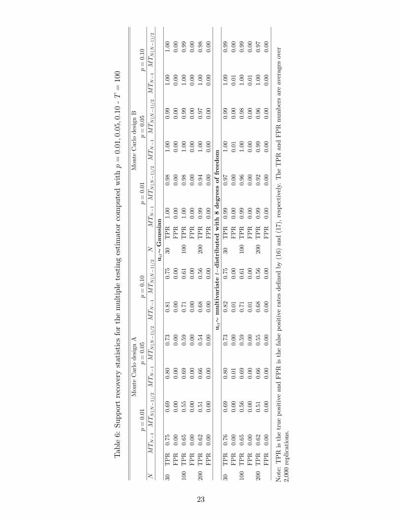
Table6:Supportrecoverystatisticsforthemultipletestingestimatorcomputedwithp=0:01;0:05;0:10-T=100

MonteCarlodesignA

MonteCarlodesignB

p=0:01

p=0:05

p=0:10

p=0:01

p=0:05

p=0:10

NMTN�1MTN(N�1)=2MTN�1MTN(N�1)=2MTN�1MTN(N�1)=2

NMTN�1MTN(N�1)=2MTN�1MTN(N�1)=2MTN�1MTN(N�1)=2

uitsGaussian

30TPR

0.75

0.69

0.80

0.73

0.81

0.75

30TPR

1.00

0.98

1.00

0.99

1.00

1.00

FPR

0.00

0.00

0.00

0.00

0.00

0.00

FPR

0.00

0.00

0.00

0.00

0.00

0.00

100TPR

0.65

0.55

0.69

0.59

0.71

0.61

100TPR

1.00

0.98

1.00

0.99

1.00

0.99

FPR

0.00

0.00

0.00

0.00

0.00

0.00

FPR

0.00

0.00

0.00

0.00

0.00

0.00

200TPR

0.62

0.51

0.66

0.54

0.68

0.56

200TPR

0.99

0.94

1.00

0.97

1.00

0.98

FPR

0.00

0.00

0.00

0.00

0.00

0.00

FPR

0.00

0.00

0.00

0.00

0.00

0.00

uitsmultivariatet�distributedwith8degreesoffreedom

30TPR

0.76

0.69

0.80

0.73

0.82

0.75

30TPR

0.99

0.97

1.00

0.99

1.00

0.99

FPR

0.00

0.00

0.01

0.00

0.01

0.00

FPR

0.00

0.00

0.01

0.00

0.01

0.00

100TPR

0.65

0.56

0.69

0.59

0.71

0.61

100TPR

0.99

0.96

1.00

0.98

1.00

0.99

FPR

0.00

0.00

0.00

0.00

0.01

0.00

FPR

0.00

0.00

0.00

0.00

0.01

0.00

200TPR

0.62

0.51

0.66

0.55

0.68

0.56

200TPR

0.99

0.92

0.99

0.96

1.00

0.97

FPR

0.00

0.00

0.00

0.00

0.00

0.00

FPR

0.00

0.00

0.00

0.00

0.00

0.00

Note:TPRisthetruepositiveandFPRisthefalsepositiveratesde�nedby(16)and(17),respectively.TheTPRandFPRnumbersareaveragesover

2,000replications.

23

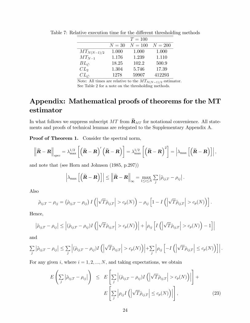
Table 7: Relative execution time for the di¤erent thresholding methodsT = 100

N = 30 N = 100 N = 200MTN(N�1)=2 1.000 1.000 1.000MTN�1 1.176 1.239 1.110BLC 18.25 102.2 500.9CL2 1.304 5.746 17.39CLC 1278 59907 412293Note: All times are relative to the MTN(N�1)=2 estimator.See Table 2 for a note on the thresholding methods.

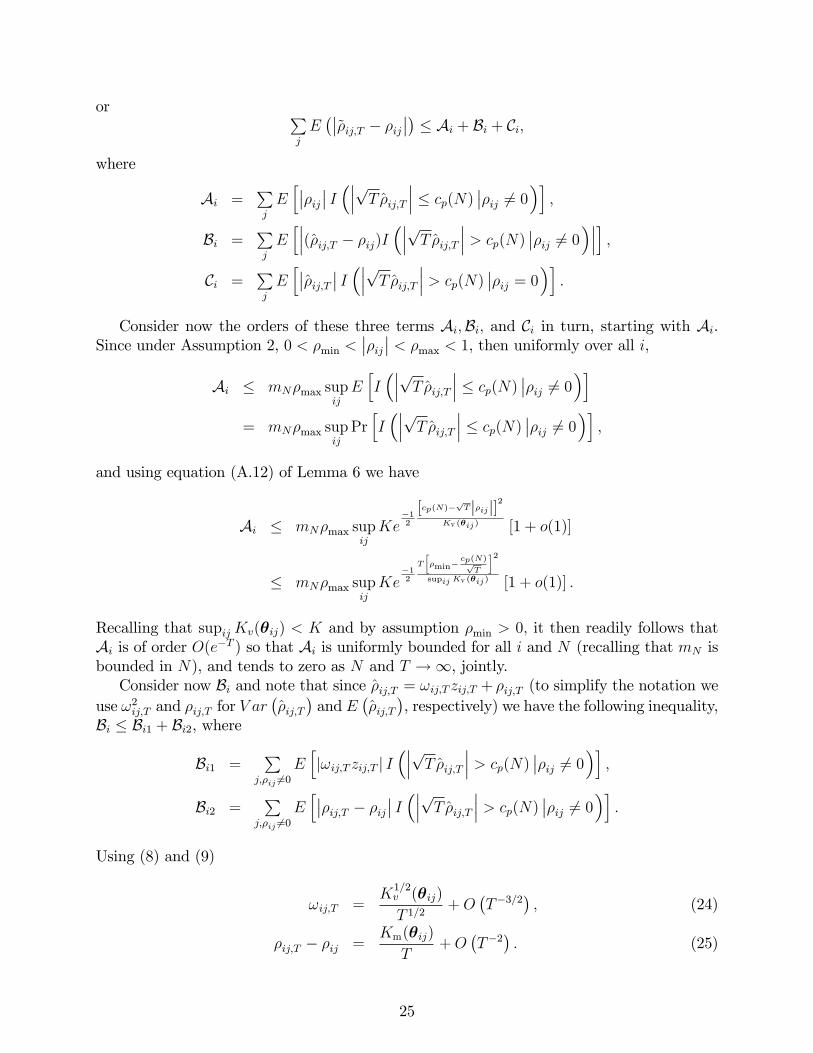
Appendix: Mathematical proofs of theorems for the MTestimator

In what follows we suppress subscript MT from eRMT for notational convenience. All state-ments and proofs of technical lemmas are relegated to the Supplementary Appendix A.

Proof of Theorem 1. Consider the spectral norm, eR�R spec

= �1=2max

��eR�R�0 �eR�R�� = �1=2max

��eR�R�2� = ��max h�eR�R�i�� ;and note that (see Horn and Johnson (1985, p.297))��max h�eR�R�i�� eR�R

1= max

1�i�N

Pj

��~�ij;T � �ij�� :

Also

~�ij;T � �ij =��ij;T � �ij

�I��pT �ij;T �� > cp(N)

�� ij

h1� I

��pT �ij;T �� > cp(N)�i:

Hence,��~�ij;T � �ij�� (�ij;T � �ij)I

��pT �ij;T �� > cp(N)��+ ��ij hI ��pT �ij;T �� > cp(N)

�� 1i��

andPj

��~�ij;T � �ij�� P

j

��(�ij;T � �ij)I��pT �ij;T �� > cp(N)

��+Pj

��ij h�I ��pT �ij;T �� cp(N)�i�� :

For any given i, where i = 1; 2; :::; N , and taking expectations, we obtain

E

Pj

��~�ij;T � �ij��! � E

"Pj

��(�ij;T � �ij)I��pT �ij;T �� > cp(N)

��#+E

"Pj

��ijI ��pT �ij;T �� cp(N)��# ; (23)

24

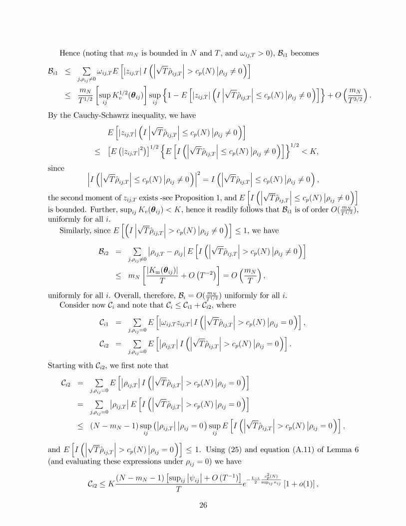
or Pj

E��~�ij;T � �ij

�� Ai + Bi + Ci;

where

Ai =Pj

Eh��ij�� I ��pT �ij;T �� cp(N)

��ij 6= 0�i ;Bi =

Pj

Eh��(�ij;T � �ij)I

��pT �ij;T �� > cp(N)��ij 6= 0��i ;

Ci =Pj

Eh��ij;T �� I ��pT �ij;T �� > cp(N)

��ij = 0�i :Consider now the orders of these three terms Ai;Bi; and Ci in turn, starting with Ai.

Since under Assumption 2, 0 < �min <��ij�� < �max < 1, then uniformly over all i,

Ai � mN�max supijEhI��pT �ij;T �� cp(N)

��ij 6= 0�i= mN�max sup

ijPrhI��pT �ij;T �� cp(N)

��ij 6= 0�i ;and using equation (A.12) of Lemma 6 we have

Ai � mN�max supijKe

�12

[cp(N)�pTj�ijj]2

Kv (�ij) [1 + o(1)]

� mN�max supijKe

�12

T

��min�

cp(N)pT

�2supij Kv (�ij) [1 + o(1)] :

Recalling that supijKv(�ij) < K and by assumption �min > 0; it then readily follows thatAi is of order O(e�T ) so that Ai is uniformly bounded for all i and N (recalling that mN isbounded in N), and tends to zero as N and T !1, jointly.Consider now Bi and note that since �ij;T = !ij;T zij;T + �ij;T (to simplify the notation we

use !2ij;T and �ij;T for V ar��ij;T

�and E

��ij;T

�, respectively) we have the following inequality,

Bi � Bi1 + Bi2, where

Bi1 =P

j;�ij 6=0Ehj!ij;T zij;T j I

��pT �ij;T �� > cp(N)��ij 6= 0�i ;

Bi2 =P

j;�ij 6=0Eh��ij;T � �ij

�� I ��pT �ij;T �� > cp(N)��ij 6= 0�i :

Using (8) and (9)

!ij;T =K1=2v (�ij)

T 1=2+O

�T�3=2

�; (24)

�ij;T � �ij =Km(�ij)

T+O

�T�2

�: (25)

25

Hence (noting that mN is bounded in N and T , and !ij;T > 0), Bi1 becomes

Bi1 �P

j;�ij 6=0!ij;TE

hjzij;T j I

��pT �ij;T �� > cp(N)��ij 6= 0�i

� mN

T 1=2

�supijK1=2v (�ij)

�supij

n1� E

hjzij;T j

�I��pT �ij;T �� cp(N)

��ij 6= 0�io+O�mN

T 3=2

�:

By the Cauchy-Schawrz inequality, we have

Ehjzij;T j


��ij 6= 0�i�

�E�jzij;T j2

��1=2 nEhI��pT �ij;T �� cp(N)

��ij 6= 0�io1=2 < K;

since ��I ��pT �ij;T �� cp(N)��ij 6= 0��2 = I

��pT �ij;T �� cp(N)��ij 6= 0� ;

the second moment of zij;T exists -see Proposition 1, and EhI��pT �ij;T �� cp(N)

��ij 6= 0�iis bounded. Further, supijKv(�ij) < K, hence it readily follows that Bi1 is of order O( mNT 1=2

),uniformly for all i.Similarly, since E

h�I��pT �ij;T �� > cp(N)

��ij 6= 0�i � 1, we haveBi2 =

Pj;�ij 6=0

��ij;T � �ij��E hI ��pT �ij;T �� > cp(N)

��ij 6= 0�i� mN

�jKm(�ij)j

T+O

�T�2

��= O

�mN

T

�;

uniformly for all i. Overall, therefore, Bi = O( mNT 1=2

) uniformly for all i.Consider now Ci and note that Ci � Ci1 + Ci2, where

Ci1 =P

j;�ij=0

Ehj!ij;T zij;T j I

��pT �ij;T �� > cp(N)��ij = 0�i ;

Ci2 =P

j;�ij=0


��ij = 0�i :Starting with Ci2, we �rst note that

Ci2 =P

j;�ij=0


��ij = 0�i=

Pj;�ij=0

��ij;T ��E hI ��pT �ij;T �� > cp(N)��ij = 0�i

� (N �mN � 1) supij

��ij;T �� ij = 0� supijEhI��pT �ij;T �� > cp(N)

��ij = 0�i ;and E

hI��pT �ij;T �� > cp(N)

��ij = 0�i � 1. Using (25) and equation (A.11) of Lemma 6

(and evaluating these expressions under �ij = 0) we have

Ci2 � K(N �mN � 1)

�supij

�� ij��+O (T�1)�

Te� 1��

2

c2p(N)

supij �ij [1 + o(1)] ;

26

where �ij =��ij(2; 2)

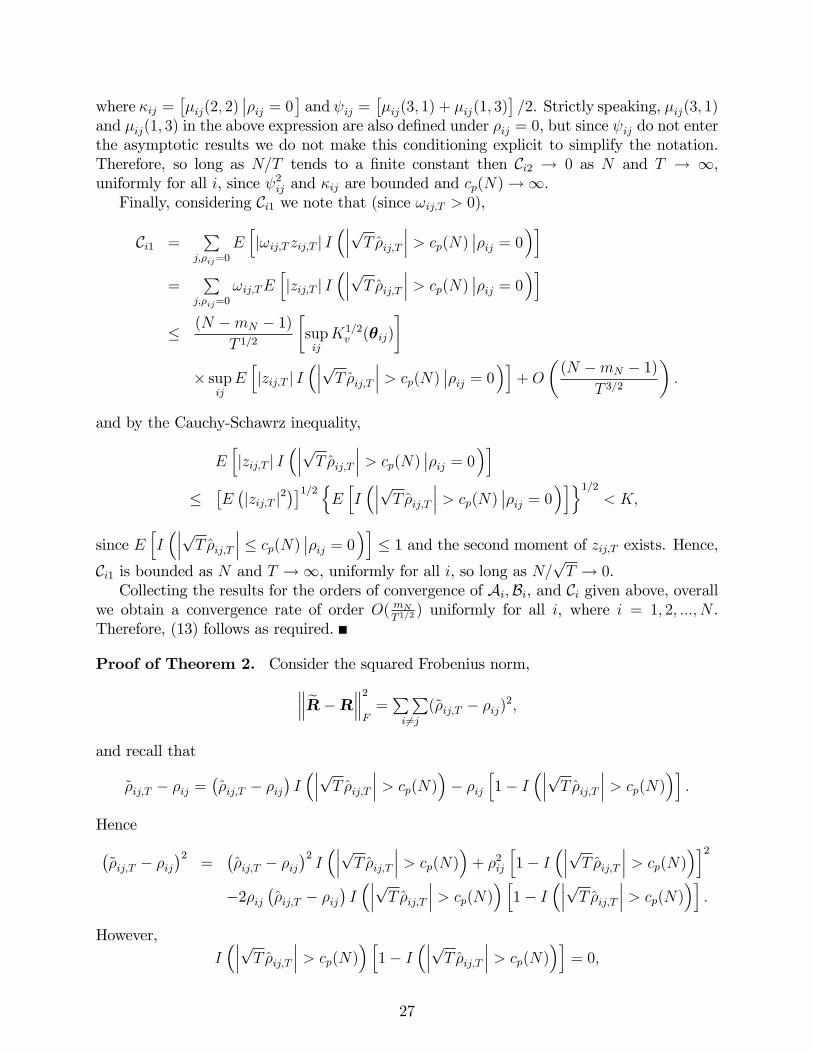
��ij = 0� and ij = ��ij(3; 1) + �ij(1; 3)� =2. Strictly speaking, �ij(3; 1)and �ij(1; 3) in the above expression are also de�ned under �ij = 0, but since ij do not enterthe asymptotic results we do not make this conditioning explicit to simplify the notation.Therefore, so long as N=T tends to a �nite constant then Ci2 ! 0 as N and T ! 1,uniformly for all i, since 2ij and �ij are bounded and cp(N)!1.Finally, considering Ci1 we note that (since !ij;T > 0),

Ci1 =P

j;�ij=0

Ehj!ij;T zij;T j I

��pT �ij;T �� > cp(N)��ij = 0�i

=P

j;�ij=0

!ij;TEhjzij;T j I

��pT �ij;T �� > cp(N)��ij = 0�i

� (N �mN � 1)T 1=2

�supijK1=2v (�ij)

�� sup

ijEhjzij;T j I

��pT �ij;T �� > cp(N)��ij = 0�i+O

�(N �mN � 1)

T 3=2

�:

and by the Cauchy-Schawrz inequality,

Ehjzij;T j I

��pT �ij;T �� > cp(N)��ij = 0�i

��E�jzij;T j2

��1=2 nEhI��pT �ij;T �� > cp(N)

��ij = 0�io1=2 < K;

since EhI��pT �ij;T �� cp(N)

��ij = 0�i � 1 and the second moment of zij;T exists. Hence,Ci1 is bounded as N and T !1, uniformly for all i, so long as N=

pT ! 0.

Collecting the results for the orders of convergence of Ai;Bi, and Ci given above, overallwe obtain a convergence rate of order O( mN

T 1=2) uniformly for all i, where i = 1; 2; :::; N .

Therefore, (13) follows as required.

Proof of Theorem 2. Consider the squared Frobenius norm, eR�R 2F=PPi6=j

(~�ij;T � �ij)2;

and recall that

~�ij;T � �ij =��ij;T � �ij

�I��pT �ij;T �� > cp(N)

�� ij

h1� I

��pT �ij;T �� > cp(N)�i:

Hence�~�ij;T � �ij

�2=

��ij;T � �ij

�2I��pT �ij;T �� > cp(N)

�+ �2ij

h1� I

��pT �ij;T �� > cp(N)�i2

�2�ij��ij;T � �ij

�I��pT �ij;T �� > cp(N)

� h1� I

��pT �ij;T �� > cp(N)�i:

However,I��pT �ij;T �� > cp(N)

� h1� I

��pT �ij;T �� > cp(N)�i= 0;

27

and h1� I

��pT �ij;T �� > cp(N)�i2

= 1� I��pT �ij;T �� > cp(N)

�:

Therefore, we havePPi6=j

�~�ij;T � �ij

�2=

PPi6=j


�2I��pT �ij;T �� > cp(N)

�+PPi6=j

�2ij

h1� I

��pT �ij;T �� > cp(N)�i

=PPi6=j


�2I��pT �ij;T �� > cp(N)

�+PPi6=j

�2ijI��pT �ij;T �� cp(N)

�;

which can be decomposed asPPi6=j

E�~�ij;T � �ij

�2= A+B + C; (26)

where

A =PPi6=j;�ij 6=0

�2ijEhI��pT �ij;T �� cp(N)

��ij 6= 0�i ;B =

PPi6=j;�ij 6=0

Eh��ij;T � �ij

�2I��pT �ij;T �� > cp(N)

��ij 6= 0�i ;C =

PPi6=j;�ij=0

Eh�2ij;T I

��pT �ij;T �� > cp(N)��ij = 0�i :

Consider now the orders of the above three terms in turn, starting with A. Since underAssumption 2, 0 < �min <

��ij�� < �max < 1, then

A � �2maxNmN supijEhI��pT �ij;T �� cp(N)

��ij 6= 0�i= �2maxNmN sup

ijPr��pT �ij;T �� cp(N)

��ij 6= 0� ;and using Lemma 6, equation (A.12), we have

A � �2maxNmN supijKe

�12

[cp(N)�pTj�ijj]2

Kv (�ij) [1 + o(1)] :

� �2maxNmN supijKe

�12

T

��min�

cp(N)pT

�2supij Kv (�ij) [1 + o(1)] :

Recalling that supijKv(�ij) < K and by assumption �min > 0; it then readily follows thatA is of order O(Ne�T ) so that A ! 0, as N and T ! 1. Note that this result does notrequire N=T ! 0, and holds even if N=T tends to a �xed constant.

28

Consider now B. Recalling that �ij;T = !ij;T zij;T + �ij;T we have the following decompo-sition of B, B = B1 +B2 + 2B3, where

B1 =PP

i6=j;�ij 6=0!2ij;TE

hz2ij;T

�I��pT �ij;T �� > cp(N)

��ij 6= 0�i ;B2 =

PPi6=j;�ij 6=0


�2Eh�I��pT �ij;T �� > cp(N)

��ij 6= 0�i ;B3 =

PPi6=j;�ij 6=0


�!ij;TE

hzij;T

�I��pT �ij;T �� > cp(N)

��ij 6= 0�i :Again, using (8) and (9)

!2ij;T =Kv(�ij)

T+O

�T�2

�; (27)�

�ij;T � �ij�2

=K2m(�ij)

T 2+O

�T�3

�; (28)


�!ij;T =

K1=2v (�ij)Km(�ij)

T 3=2+O

�T�5=2

�: (29)

Hence (noting that mN is bounded in N and T )

B1 =PP

i6=j;�ij 6=0!2ij;TE

hz2ij;T

�I��pT �ij;T �� > cp(N)

��ij 6= 0�i� NmN

T

�supijKv(�ij)

�supij

n1� E

hz2ij;T


��ij 6= 0�io+O

�mNN

T 2

�:

Since supijKv(�ij) and Ehz2ij;T


��ij 6= 0�i are bounded, it then readilyfollows thatB1 is at mostO

�NmNT

�. In fact limT!1E

hz2ij;T

�I��pT �ij�� cp(N)

��ij 6= 0�i =0 if

pT�min � cp(N)!1, as N and T !1, which can be easily shown.

Similarly, since Eh�I��pT �ij;T �� > cp(N)

��ij 6= 0�i � 1, we haveB2 =

PPi6=j;�ij 6=0


�2Eh�I��pT �ij;T �� > cp(N)

��ij 6= 0�i� NmN

�K2m(�ij)

T 2+O

�T�3

��= O

�NmN

T 2

�;

and

B3 =PPi6=j;�ij 6=0


�!ij;TE

nzij;T

hI��pT �ij;T �� > cp(N)

��ij 6= 0�io=

PPi6=j;�ij 6=0


�!ij;TE

nzij;T � zij;T

hI��pT �ij;T �� cp(N)

��ij 6= 0�io= �

PPi6=j;�ij 6=0


�!ij;TE

hzij;T I

��pT �ij;T �� cp(N)��ij 6= 0�i : (30)

29

Also, from Lemma 4

limT!1

Ehzij;T I

��pT �ij;T �� cp(N)��ij 6= 0�i = lim

T!1E�zI�Lij;T � z � Uij;T

��ij 6= 0�� ;and from Lemma 2

E�zI�Lij;T � z � Uij;T

��ij 6= 0�� = �

0@�cp(N)�pT�ij +O�

1pT

�qKv(�ij) +O

�1T

�1A

��

0@cp(N)�pT�ij +O�

1pT

�qKv(�ij) +O

�1T

�1A ; (31)

which is bounded in N and T . SincepT�min � cp(N) ! 1 as N and T ! 1, it is easily

seen that limT;N!1E�zI�Lij;T � z � Uij;T

��ij 6= 0�� = 0. Hence, using (29) and noting

that K1=2v (�ij)Km(�ij) is bounded in T we have

B3 � KPPi6=j;�ij 6=0

��ij;T � �ij�!ij;T

�� = O

�NmN

T 3=2

�:

Overall, therefore, B = O�NmNT

�.

Consider now the following decomposition of C, in (26):

C =PPi6=j;�ij=0

Eh�2ij;T I

��pT �ij;T �� > cp(N)��ij = 0�i

=PPi6=j;�ij=0

!2ij;TEhz2ij;T I

��pT �ij;T �� > cp(N)��ij = 0�i

+PPi6=j;�ij=0

�2ij;TEhI��pT �ij;T �� > cp(N)

��ij = 0�i+2PP

i6=j;�ij=0�ij;T!ij;TE

hzij;T I

��pT �ij;T �� > cp(N)��ij = 0�i

= C1 + C2 + C3:

Starting with the simpler terms, we �rst note that

C2 =PPi6=j;�ij=0

�2ij;TEhI��pT �ij;T �� > cp(N)

��ij = 0�i� N(N �mN � 1) sup

ij

��2ij;T

��ij = 0� supijEhI��pT �ij;T �� > cp(N)

��ij = 0�i ;and supij E

hI��pT �ij�� > cp(N)

��ij = 0�i � 1. Using (8) and equation (A.11) of Lemma6 (and evaluating these expressions under �ij = 0) we have

C2 � KN(N �mN � 1) supij

� 2ij +O (T�1)

�T 2

e� 1��

2

c2p(N)

supij �ij [1 + o(1)] ;

30

where �ij =��ij(2; 2)

��ij = 0�, and ij = ��ij(3; 1) + �ij(1; 3)

�=2. Therefore, so long as

N=T tends to a �nite constant then C2 ! 0 as N and T !1, since 2ij and �ij are boundedand cp(N)!1.Similarly

C3 =PPi6=j;�ij=0

�ij;T!ij;TEhzij;T I

��pT �ij;T �� > cp(N)��ij = 0�i

= �PP

i6=j;�ij=0�ij;T!ij;TE

hzij;T I

��pT �ij;T �� cp(N)��ij = 0�i

� N(N �mN � 1)T 3=2

supij

�� ij��+O�T�1

��supij

�p�ij +O

�T�1

�� sup

ijEhzij;T I

��pT �ij;T �� cp(N)��ij = 0�i :

But using Lemma 4, Lemma 2 and (31) and evaluating the relevant expressions under �ij = 0,we have

limT;N!1

Ehzij;T I

��pT �ij;T �� cp(N)��ij = 0�i

= limT;N!1

E�zI�Lij;T � z � Uij;T

��ij = 0��= lim

N;T!1�

0@�cp(N) + ijpT+O

�T�3=2

�q�ij +O

�1T

�1A� lim

N;T!1�

0@cp(N) + ijpT+O

�T�3=2

�q�ij +O

�1T

�1A = 0:

Hence, C3 ! 0 as N and T !1, so long as N=pT ! 0, since cp(N)!1 with N .

Finally, considering C1 we note that

C1 =PPi6=j;�ij=0

!2ij;TEhz2ij;T I

��pT �ij;T �� > cp(N)��ij = 0�i

=PP

i6=j;�ij=0!2ij;TE

�z2ij;T

�1� I

�Lij;T � zij;T � Uij;T

��ij = 0�� N(N �mN � 1)

Tsupij

��ij +O

�1

T

�� sup

ijE�z2ij;T

�1� I


��ij = 0�� : (32)

But using Lemma 4

limT!1

E�z2ij;T

�1� I


��ij = 0�� (33)

= limT!1

E�z2�1� I


��ij = 0�� ;and then Lemma 2

E�z2�1� I


��ij = 0�� = 1� E�z2I�Lij;T � z � Uij;T

��ij = 0��= 1� f� [Uij;T (0)]� � [Lij;T (0)] + Lij;T (0)�(Lij;T (0))� Uij;T (0)� [Uij;T (0)]g= � [�Uij;T (0)] + � [Lij;T (0)] + Uij;T (0)� [Uij;T (0)]� Lij;T (0)� [Lij;T (0)] ;

31

where Uij;T (0) and Lij;T (0) are given by (A.19) which we reproduce here for convenience:

Uij;T (0) =cp(N) +

ijpT+O

�T�3=2

�p�ij +O (T�1)

, Lij;T (0) =�cp(N) +

ijpT+O

�T�3=2

�p�ij +O (T�1)

:

Since�� ij�� < K, then there existN0 and T0 such that forN > N0 and T > T0, cp(N)�

j ijjpT>

0, and using Lemma 5 (also see (A.23) and (A.24) of Lemma 6), we have

E�z2�1� I

�Lij;T � z � Uij;T

��ij = 0�� D1;ij +D2;ij;

where

D1;ij =1

2e

�12

0@ cp(N)+ ijpT+O(T�3=2)p

�ij+O(T�1)

1A2

+1

2e

�12

0@ cp(N)� ijpT+O(T�3=2)p

�ij+O(T�1)

1A2

;

and

D2;ij =

24cp(N) + ijpT+O

�T�3=2

�p�ij +O (T�1)

35 e�120@ cp(N)+

ijpT+O(T�3=2)p

�ij+O(T�1)

1A2

�

24�cp(N) + ijpT+O

�T�3=2

�p�ij +O (T�1)

35 e�120@ cp(N)�

ijpT+O(T�3=2)p

�ij+O(T�1)

1A2

:

Then, for N D1;ij we have

limN;T!1

N D1;ij = limN!1

"e�12

c2p(N)

�ij+ln(N)

#

= limN!1

"e� ln(N)�ij

�c2p(N)

2 ln(N)��ij

�#:

Since �ij > 0, then N D1;ij tends to a �nite constant or zero if limN!1

�c2p(N)

2 ln(N)

�� ij. But

using (A.6) of Lemma 3, we have

ln [f(N)]� ln(p)ln(N)

�c2p(N)

2 ln(N)� �max;

where �max = supij(�ij). Next, for N D2;ij we have

N D2;ij =

24Ncp(N) + N ijpT+O

�NT�3=2

�p�ij +O (T�1)

35 e�1224 cp(N)+ ijp

T+O(T�3=2)p

�ij+O(T�1)

352

�

24�Ncp(N) + N ijpT+O

�NT�3=2

�p�ij +O (T�1)

35 e�1224 cp(N)� ijp

T+O(T�3=2)p

�ij+O(T�1)

352;

32

or

N D2;ij =

241 + ij

cp(N)pT+O

�N�1T�3=2

�p�ij +O (T�1)

35 e�� ln(N)�ij

�c2p(N)

2 ln(N)��ij

�1+

ln(cp(N))

ln(N)

��

+

241� ij

cp(N)pT+O

�N�1T�3=2

�p�ij +O (T�1)

35 e�� ln(N)�ij

�c2p(N)

2 ln(N)��ij

�1+

ln(cp(N))

ln(N)

��:

Then N D2;ij tends to a �nite constant for all i and j as long asln(cp(N))

ln(N)! c. Hence, for

N=T tending to a constant and using the above results in (32) we have

C1 �(N �mN � 1)

Tsupij

��ij +O

�T�1

��supij(ND2;ij) :

Hence, C1 must be at most O(N=T ); since by assumption limN!1ln[f(N)]ln(N)

� �max.Collecting the results for the orders of convergence of C1; C2, and C3 given above, and

those of A and B, overall we obtain a convergence rate of order O(mNN=T ), and (15) followsas desired.

Proof of Theorem 3. Consider �rst the FPR statistic given by (17) which can be writtenequivalently as

FPR = jFPRj =

PPi6=j

I��pT �ij;T �� > cp(N)j�ij = 0

�N(N �mN � 1)

: (34)

Note that the elements of FPR are either 0 or 1 and so jFPRj = FPR:Taking the expectation of (34) we have

E jFPRj =

PPi6=j

Pr��pT �ij;T �� > cp(N)j�ij = 0

�N(N �mN � 1)

:

But using Lemma 6 (equation (A.11)) we have (recall that �ij =��ij(2; 2)

��ij = 0�)E jFPRj �

KPPi6=j

e� 1��

2

c2p(N)

�ij [1 + o(1)]

N(N �mN � 1)

� Ke�1��2

c2p(N)

�max [1 + o(1)]

where �max = supij �ij < K, by Assumption 2. Hence, E jFPRj ! 0 as N and T ! 1,noting that c2p(N)!1, and �max < K. Further, by the Markov inequality applied to jFPRjwe have that

P (jFPRj > �) � E(jFPRj)�

� K

�e�

1��2

c2p(N)

�max [1 + o(1)] ;

33

for some � > 0: Therefore, limN;T!1

P (jFPRj > �) = 0; and the required result is established.

This holds irrespective of the order by which N and T !1.Consider now the TPR statistic given by (16) and note that

TPR =

PPi6=j

I(~�ij 6= 0; and �ij 6= 0)PPi6=j

I(�ij 6= 0)

Hence

X = 1� TPR =

PPi6=j

I(~�ij = 0; and �ij 6= 0)

NmN

:

Since jXj = X, then

E jXj = E(X) =

PPi6=j

Pr��pT �ij;T �� < cp(N)j�ij 6= 0

�NmN

� supijPr��pT �ij;T �� < cp(N)j�ij 6= 0

�:

and using the Markov inequality, P (jXj > �) � EjXj�, for some � > 0, we have

P (jTPR� 1j > �) � 1

�supijPr��pT �ij;T �� < cp(N)j�ij 6= 0

�;

andlim

N;T!1P (jTPR� 1j > �) � 1

�lim

N;T!1supijPr��pT �ij;T �� < cp(N)j�ij 6= 0

�: (35)

However, using (A.25), (A.26) and (A.27) of Lemma 6 we have


�= Fij;T

cp(N)�

pT�ij �

Km (�ij)pT

+O�T�3=2

�pKv(�ij) +O (T�1)

!

�Fij;T

�cp(N)�

pT�ij �

Km (�ij)pT

+O�T�3=2

�pKv(�ij) +O (T�1)

!:

Suppose that �ij > 0, then as N and T !1, cp(N)�pT�ij ! �1 and �cp(N)�

pT�ij !

�1, and since Fij;T (�) is a cumulative distribution function we must have

limN;T!1


�= Fij;T (�1)� Fij;T (�1) = 0� 0 = 0.

Similarly if �ij < 0, then cp(N)�pT�ij ! +1 and �cp(N)�

pT�ij ! +1, and we have

limN;T!1


�= Fij;T (+1)� Fij;T (+1) = 1� 1 = 0.

34

Hence, more generally limN;T!1 Pr��pT �ij;T �� < cp(N)j�ij 6= 0

�= 0, if cp(N)�

pT��ij��!

�1, for all �ij 6= 0, or equivalently ifpT�min � cp(N) ! 1, where �min = minij

��ij�� for�ij 6= 0. But

pT�min � cp(N) =

pT

��min �

cp(N)pT

�;

andpT�min � cp(N) ! 1, as N and T , since by assumption there exists N0 and T0 such

that for all N > N0 and T > T0, �min � cp(N)=pT > 0, and cp(N)=

pT ! 0. The latter is

ensured since by assumption ln f(N)=T ! 0 (see also Lemma 3). Using these results in (35)it now follows that limN;T!1 P (jTPR� 1j > �)! 0; as required.

ReferencesAbadir, K. M., Distaso, W. and Zikes, F. (2014). Design-free estimation of large variance matrices. Journal

of Econometrics, forthcoming.

Bickel, P. J. and Levina, E. (2004). Some theory for Fisher�s linear discriminant function, �naive Bayes�, and

some alternatives when there are many more variables than observations. Bernoulli, 10, 989�1010.

Bickel, P. J. and Levina, E. (2008a). Regularised estimation of large covariance matrices. The Annals of

Statistics, 36, 199�227.

Bickel, P.J. and Levina, E (2008b). Covariance regularisation by thresholding. The Annals of Statistics, 36,

2577�2604.

Bonferroni, C. (1935). Il calcolo delle assicurazioni su gruppi di teste. Studi in Onore del Professore Salvatore

Ortu Carboni, Rome, Italy, 13�60.

Cai, T. and Liu, W. (2011). Adaptive thresholding for sparse covariance matrix estimation. Journal of

American Statistical Association, 106, 672�684.

Carroll, R. J. (2003). Variances are not always nuissance parameters. Biometrics, 59, 211�220.

Daniels, M. J. and Kass, R. (1999). Nonconjugate Bayesian estimation of covariance matrices in hierarchical

models. Journal of American Statistical Association, 94, 1254�1263.

Daniels, M. J. and Kass, R. (2001). Shrinkage estimators for covariance matrices. Biometrics, 57, 1173�1184.

D�Aspremont, A., Banerjee, O. and Elghaoui, L. (2008). First-order methods for sparse covariance selection.

SIAM Journal on Matrix Analysis and Applications, 30, 56�66.

Dees, S., di Mauro, F., Pesaran, M. H. and Smith, L.V. (2007). Exploring the international linkages of the

euro area: A Global VAR Analysis. Journal of Applied Econometrics, 22, 1�38.

El Karoui, N. (2008). Operator norm consistent estimation of large dimensional sparse covariance matrices.

The Annals of Statistics, 36, 2717�2756.

Fan, J., Fan, Y. and Lv, J. (2008). High dimensional covariance matrix estimation using a factor model.

Journal of Econometrics, 147, 186�197.

Fan, J., Li, R. (2001). Variable selection via nonconcave penalized likelihood and its oracle properties.

Journal of American Statistical Association, 96, 1348�1360.

Fan, J., Liao, Y. and Mincheva, M. (2011). High dimensional covariance matrix estimation in approximate

factor models. The Annals of Statistics, 39, 3320�3356.

35

Fan, J., Liao, Y. and Mincheva, M. (2013). Large covariance estimation by thresholding principal orthogonal

complements. Journal of Royal Statistical Society, Series B, 75, 1�44.

Friedman, J. H. (1989). Regularized discriminant analysis. Journal of the American Statistical Association,

84, 165�175.

Fryzlewicz, P. (2013). High-dimensional volatility matrix estimation via wavelets and thresholding. Bio-

metrika, 100, 921�938.

Gayen, A. K. (1951). The frequency distribution of the product-moment correlation coe¢ cient in random

samples of any size drawn from non-normal universes. Biometrika, 38, 219-247.

Ho¤, P. D. (2009). A hierarchical eigenmodel for pooled covariance estimation. Journal of Royal Statistical

Society, Series B, 71, 971�992.

Holm, S. (1979). A simple sequentially rejective multiple test procedure. Scandinavian Journal of Statistics,

6, 65�70.

Horn, R. A. and Johnson, C. R. (1985). Matrix analysis. Cambridge University Press: Cambridge.

Ledoit, O. and Wolf, M. (2003). Improved estimation of the covariance matrix of stock returns with an

application to portfolio selection. Journal of Empirical Finance, 10, 603�621.

Ledoit O. and Wolf, M. (2004). A well-conditioned estimator for large-dimensional covariance matrices.

Journal of Multivariate Analysis, 88, 365�411.

Liu, H., Wang, L. and Zhao, T. (2013). Sparse covariance matrix estimation with eigenvalue constraints.

Journal of Computational and Graphical Statistics. DOI:10.1080/10618600.2013.782818.

Peng, J., Wang, P., Zhou, N. and Zhu, J. (2009). Partial correlation estimation by joint sparse regression

models. Journal of American Statistical Association, 104, 735�746.

Pesaran, M. H. (2015). Testing weak cross-sectional dependence in large panels. Econometric Reviews, 34,

1089�1117.

Pesaran M. H., Schuermann, T. and Weiner, S. M. (2004). Modeling regional interdependencies using a

Global Error Correcting Macroeconometric model. Journal of Business & Economic Statistics, 22, 129�162.

Pourahmadi, M. (1999). Joint mean-covariance models with applications to longitudinal data: Unconstrained

parameterisation. Biometrika, 86, 677�690.

Pourahmadi, M. (2000). Maximum likelihood estimation of generalised linear models for multivariate normal

covariance matrix. Biometrika, 87, 425�435.

Pourahmadi, M. (2011). Covariance estimation: GLM and regularisation perspectives. Statistical Science,

26, 369�387.

Romano, P. J. and Wolf, M. (2005). Exact and approximate stepdown methods for multiple hypothesis

testing. Journal of the American Statistical Association, 100, 469, 94�108.

Romano, P. J. Shaikh, A. M. and Wolf, M. (2008). Formalised data snooping based on generalised error

rates. Econometric Theory, 24, 404�447.

Rothman, A. J. (2012). Positive de�nite estimators of large covariance matrices. Biometrika, 99, 733�740.

Rothman, A. J., Bickel, P. J., Levina, E. and Zhu, J. (2008). Sparse permutation invariant covariance

estimation. Electronic Journal of Statistics, 2, 494�515.

Rothman, A. J., Bickel, P. J., Levina, E. and Zhu, J. (2010). A new approach to Cholesky-based estimation

of high-dimensional covariance matrices. Biometrika, 97, 539�550.

Rothman, A. J., Levina, E. and Zhu, J. (2009). Generalised thresholding of large covariance matrices.

Journal of American Statistical Association, 104, 177�186.

36

Sargan, J. D. (1976). Econometric estimators and the edgeworth approximation. Econometrica, 44(3),

421�448.

Schäfer, J. and Strimmer, K. (2005). A shrinkage approach to large-scale covariance matrix estimation and

implications for functional Genomics. Statistical Applications in Genetics and Molecular Biology, 4, Article

32.

Sentana, E. (2009). The econometrics of mean-variance e¢ ciency tests: A survey. The Econometrics Journal,

12, 65�101.

Tschuprow, A. (1925). Grundbegri¤e und grundprobleme der korrelationstheorie. Leipzig: B.G. Teubner.

Wu, W. B. and Pourahmadi, M. (2009). Banding sample covariance matrices for stationary processes.

Statistica Sinica, 19, 1755�1768.

Xue, L., Ma, S. and Zou, H. (2012). Positive-de�nite `1-penalized estimation of large covariance matrices.Journal of the American Statistical Association, 107, 1480�1491.

Yuan, M. and Lin, Y. (2007). Model selection and estimation in the Gaussian graphical model. Biometrika,

94, 19�35.

Zou, H. (2006). The adaptive lasso and its oracle properties. Journal of American Statistical Association,

101, 1418�1429.

37

Documents

A multiple testing approach to the regularisation of large ... · A multiple testing approach to the regularisation of large sample correlation matrices ... (Fan et al. (2008)) and