A multiparametric method of interpolation using …digital.csic.es/bitstream/10261/33619/1/A.Velo.pdf · en el Atlántico, calculado por dos métodos de estimación sobre la base

A multiparametric method of interpolation using WOA05 applied to anthropogenic CO2 in the Atlantic

ANTON VELO, MARCOS VÁZQUEZ-RODRÍGUEZ, XOSE A. PADÍN, MIGUEL GILCOTO, AÍDA F. RÍOS and FIZ F. PÉREZ

Instituto de Investigacións Mariñas (CSIC). Eduardo Cabello 6, 36208 Vigo, Spain. E-mail: [email protected]

SUMMARY: This paper describes the development of a multiparametric interpolation method and its application to anthro-pogenic carbon (CANT) in the Atlantic, calculated by two estimation methods using the CARINA database. The multiparamet-ric interpolation proposed uses potential temperature (θ), salinity, conservative ‘NO’ and ‘PO’ as conservative parameters for the gridding, and the World Ocean Atlas (WOA05) as a reference for the grid structure and the indicated parameters. We thus complement CARINA data with WOA05 database in an attempt to obtain better gridded values by keeping the physical-biogeochemical sea structures. The algorithms developed here also have the prerequisite of being simple and easy to implement. To test the improvements achieved, a comparison between the proposed multiparametric method and a pure spatial interpolation for an independent parameter (O2) was made. As an application case study, CANT estimations by two methods (jCTº and TrOCA) were performed on the CARINA database and then gridded by both interpolation methods (spatial and multiparametric). Finally, a calculation of CANT inventories for the whole Atlantic Ocean was performed with the gridded values and using ETOPO2v2 as the sea bottom. Thus, the inventories were between 55.1 and 55.2 Pg-C with the jCTº method and between 57.9 and 57.6 Pg-C with the TrOCA method.

Keywords: CARINA, WOA05, CO2, interpolation, multiparametric, anthropogenic carbon, back calculation.

RESUMEN: Un método multiparamétrico de interpolación utilizando WOA05, aplicado al CO2 antropogéni-co en el Atlántico. – Este trabajo describe el desarrollo de un método de interpolación multiparamétrico, y su aplicación al carbono antropogénico CANT en el Atlántico, calculado por dos métodos de estimación sobre la base de datos de CARINA. La interpolación multiparamétrica propuesta utiliza temperatura potencial (θ), salinidad, ‘NO’ y ‘PO’ conservativo a modo de parámetros conservativos para el mallado, y el World Ocean Atlas (WOA05) como referencia tanto para la estructura de la malla, como para los parámetros indicados. De este modo, este trabajo complementa CARINA con la base de datos de WOA05, intentando obtener mejores valores interpolados por el hecho de mantener las estructuras físico-biogeoquímicas marinas. Además, los algoritmos desarrollados tienen el prerrequisito de ser sencillos y fáciles de implementar. Para compro-bar las mejoras conseguidas, se ha realizado una comparación de un parámetro independiente (O2) entre el método multipa-ramétrico y una interpolación puramente espacial. A modo de estudio de un caso de aplicación, se han realizado estimaciones de CANT mediante dos métodos (jCTº and TrOCA) sobre la base de datos de CARINA, y posteriormente interpolado mediante ambos métodos de interpolación (espacial y multiparamétrica). Por último, se ha realizado un cálculo de los inventarios de CANT para el Océano Atlántico completo con los valores interpolados y utilizando ETOPO2v2 como fondo marino. De este modo los inventarios obtenidos fueron de entre 55.1 y 55.2 PgG con la aproximación jCTº, y entre 57.9 y 57.6 Pg-C con la aproximación TrOCA.

Palabras clave: CARINA, WOA05, CO2, intepolación, multiparamétrico, carbono antropogénico, retrocálculo.

Scientia Marina 74S1December 2010, 21-32, Barcelona (Spain)

ISSN: 0214-8358doi: 10.3989/scimar.2010.74s1021

INTRODUCTION

This work began as a contribution to the CARINA (Carbon in the Atlantic Ocean) Project, with the aim of developing an interpolation algorithm that would

enhance the gridding in low coverage areas, but with the premise of being easy to apply. The algorithm would also help to build a large and comprehensive carbon system database for the Atlantic Ocean with the CARINA database. The development should con-

ADVANCES IN MARINE CHEMISTRYJ. Blasco and J.M. Forja (eds.)

22 • A. VELO et al.

SCI. MAR., 74S1, December 2010, 21-32. ISSN 0214-8358 doi: 10.3989/scimar.2010.74s1021

tribute to estimate the CANT inventory of this ocean by, as part of a future work, gridding the CANT that can be calculated with the available approximation methods. Finally, the interpolation method could be used in the CARINA project to help to get the gridded product from the other available CARINA parameters. The interpolation algorithms developed here pursue the goal of being simple and easy to implement. After the seminal work of Gandin (1965) introducing objective analysis to produce gridded maps of meteorological variables in a systematic manner, objective interpola-tion methods were transferred from meteorology to oceanography in the late 1970s (Bretherton et al., 1976; Freeland and Gould, 1976; Jalickee and Ham-ilton, 1977). Today, objective analysis appears in standard oceanography texts such as Bennett (1992) and Emery and Thomson (2001). In fact, one of the databases used in the present study, the World Ocean Atlas (WOA05, see Material and Methods section), was processed with these data analysis techniques. The present study uses a multiparametric inverse distance algorithm that was applied to the CARINA data (see the Material and Methods section) and took the WOA05 objective interpolated data as a reference to calculate the multiparametric distances. This ap-proach provides a simple interpolation algorithm that is easy to use and to quality assess.

The CARINA Project has fed its dataset only from cruises in which carbon parameters were measured, so data coverage is low in certain regions, such as the Southern Ocean. Within this context, an interpolation method based only on geographical distances might perform poorly precisely on these regions due to the sparseness. A possible way to alleviate this problem is to incorporate more information in the interpola-tion algorithm other than the spatial. Thus, the con-sideration of fields of conservative properties for different water masses would become a benefit in this regard, providing better fits to real distributions than those generated from a purely spatial distance–based method. One additional advantage of this procedure is that the artefacts that may appear in the water mass distributions derived from plain spatial interpolations could be avoided.

The CARINA dataset is not distributed over a structured uniform grid, but is rather composed mainly from dispersed CTD stations organized in transoceanic sections. In terms of recorded variables, the dataset compiles many biogeochemical parame-ters, including the ones needed for the calculation of CANT by different methods. In contrast, the WOA05 dataset is structured in a homogenous three dimen-sional grid with thermohaline and biogeochemical variables defined at the nodes of the grid, but it lacks many of the parameters needed for carbon calcula-tions. Therefore, the generation of a multiparametric interpolation algorithm that combines the properties of the WOA05 and CARINA datasets appears to be the logical way to proceed. Applying this to CANT es-

timation should provide CANT interpolated data over the structured WOA05 grid, taking advantage of the common hydrographical information available in both datasets.

As a way to evaluate the results, two versions of the interpolation method were compared; one based only on spatial distances and one that uses the physical and biogeochemical tracers (hereafter referred to as the Water Mass Properties [WMP] interpolation method). The contrast of the individual behaviour of the two methods was carried out using dependent variables (in-terpolating variables included in the multiparametric distances) and one independent variable (oxygen, not included in the multiparametric distances).

As the quality tests of the WMP interpolation method yield positive results, a step forward was taken: interpolating anthropogenic carbon over the WOA05 grid. The major role played by the oceans in the global carbon cycle is incontrovertible, since they have the capacity to sequestrate 2.2±0.4 Pg C per year, roughly a 25% of the total anthropogenic carbon (CANT) emit-ted to the atmosphere (8.0±0.5 Pg yr-1) (Canadell et al., 2007). Most outstandingly, the Atlantic Ocean stores 38% of the oceanic anthropogenic carbon (Sabine et al., 2004), though it represents 29% of the global ocean surface area. The particular dynamics of the Atlantic Ocean allows the formation of deep waters in the North Atlantic and this enhances the uptake fluxes and storage capacity of CANT of this basin. Recently detected proc-esses triggered by decadal changes of global climate, such as the slowdown of the Meridional Overturning Circulation, seem to have contributed significantly to reducing the sink capacity of CANT in both the North Atlantic and the Southern Ocean (Joos et al., 1999; Le Quéré et al., 2007). The juxtaposition of these op-. The juxtaposition of these op-posed effects has dramatically magnified the need to accurately estimate the state of CANT inventories and has raised the importance of fine-tuning the CANT inter-polation methods applied to sparse or geographically disperse datasets.

Two methods were used to obtain the estimation of CANT over the whole Atlantic Ocean, jCTº and TrOCA. The jCTº estimation method was chosen as it was developed by the authors (Vázquez-Rodríguez et al., 2009a) and it was straightforward to apply and verify (the MATLAB script is publicly available for down-load at http://oceano.iim.csic.es/co2group/). It is also an updated method and seems to perform well in com-parison with other methods (Vázquez-Rodríguez et al., 2009b). The TrOCA method (Touratier et al., 2007) was additionally considered as a support reference due to its ease of application. Consequently, anthropogenic carbon was calculated by applying these estimations to the CARINA dataset, and then gridded by both the WMP and Spatial interpolation methods. The next step taken was to calculate the volumes in order to obtain the inventories. ETOPO2v2 (U.S. Department of Com-(U.S. Department of Com-merce, 2006) was chosen as reference for the ocean floor in these calculations.

MULTIPARAMETRIC INTERPOLATION WITH WOA APPLIED TO CANT • 23


MATERIALS AND METHODS

Database

CARINA is a database of comprehensive carbon data, sourced from hydrographic cruises conducted in the Arctic, Atlantic and Southern Oceans. The project was initiated in 1999 as an essentially informal and unfunded project in Kiel, Germany, with the main goal of creating a database of relevant carbon variables to be used for accurate assessments of carbon inventories, transports and uptake rates. The CARINA data have been gathered from various sources and then put under rigorous quality controls (QC) to produce a consistent data product. Experience with previous synthesis ef-forts like the Global Data Analysis Project (GLODAP) (Key et al., 2004) demonstrated that a consistent data product can be achieved from different cruises, per-formed by different laboratories and in very different regions. The CARINA database includes data and metadata from 188 oceanographic cruises or projects, (Hoppema et al., 2009; Tanhua et al., 2009; Key et al., 2010; Tanhua et al., 2010). In addition, 52 WOCE/GLODAP cruises were included in the quality control to ensure consistency with historical data. Parameters included in the CARINA dataset are salinity (S), po-tential temperature (θ), oxygen (O2), nitrate (NO3), phosphate (PO4), silicate (SiO4), total alkalinity (AT), fugacity of carbon dioxide (fCO2), total inorganic car-bon (CT), pH, CFC-11, CFC-12, CFC-113 and CCl4. Due to the different origins of the data, the data density has heterogeneous distributions, being scarcer in the South Atlantic than in the North Atlantic.

The World Ocean Atlas 2005 (WOA05) has widely proven its usefulness to the oceanographic and atmospheric research communities. WOA05 of-fers a gridded database interpolated from many dif-ferent sources by oceanographic objective analysis techniques. The WOA05 climatological analyses were carried out on a 1º × 1º grid. This comes from the fact that higher resolution analyses are not justi-fied for all the measured properties, and they should be analyzed in the same manner. For a description of the WOA05 data and statistical fields, refer to http://www.nodc.noaa.gov/OC5/WOA05/pubwoa05.html. The site includes a list of values and statistical data in a one-degree latitude-longitude world grid (360 × 180) at 33 standard depth levels from the surface to a maximum depth of 5500 m.

The WOA05 series include analysis of temperature (Locarnini et al., 2006), salinity (Antonov et al., 2006), dissolved oxygen, apparent oxygen utilization, oxygen saturation (Garcia et al., 2006a), and dissolved inor-, and dissolved inor-ganic nutrients (Garcia et al., 2006b). The climatolo-. The climatolo-gies defined here come from historical oceanographic profiles and selected data at different depths. Data used in the WOA05 were analyzed in a consistent, objec-tive analysis mode and interpolated over a one-degree latitude-longitude grid at standard depth levels.

The aim of the WOA05 maps is to illustrate the large-scale characteristics of the distribution of ocean temperature. The fields used to generate these climato-logical maps were computed by objective analysis of quality-controlled historical temperature data. Maps are presented for climatological composite periods (annual, seasonal, monthly, and monthly difference fields from the annual mean field, and the number of observations) at selected standard depths. The annual climatology was calculated using all data regardless of the month of the observation. Seasonal climatologies were calculated using only data from the defined sea-son (regardless of year). However, in this study only the annual maps for the whole Atlantic Ocean (Lat: 90ºS-90ºN, Lon: 81ºW-33ºE) were used.

For the CANT inventory calculations, the ETOPO2v2 (USDC, NOAA, NGDC 2006) bathymetry was used as bottom reference to calculate the volume of the deepest boxes.

Interpolation Method

Hereafter var is the parameter that we wish to inter-polate. The objective is to obtain for each node j of the structured WOA05 grid an average value of var, which is unavailable from this database. The known values of var from the CARINA unstructured-grid nodes i will be used to fill in the j WOA05 nodes. A classic inter-polation scheme of inverse distance is applied, using a weighted estimation of the i neighbouring samples to the j WOA05 node:

varvar

j

i ij

i

ij

i

f

f=

( )( )

−

−

∑∑

1

1 (1)

The weighting factors used in the basic spatial in-terpolation are defined by:

f wlat lat

la∆ ∆

∆

tw

lon lon

lonij

lat

i j

lon

i j

=−

+−

2

+

+−

+−

( )

2

2

wz z

zw

stdz

i j i j

jθ

θ θθ

+−

( )+

+−

( )

2 2

wS S

std S

wNO NO

std NO

S

i j

j

NO

i j

j+

−

( )

2 2

wPO PO

std POPO

i j

j

(2)

where several variables are pondered with arbitrary weights (wx). The specific values of the wx terms to produce the fi

j factors are subjected to the criteria of the researcher. The information concerning the geographi-cal position is taken into account in the interpolation through the spatial coordinates of longitude (lon), latitude (lat) and depth (z). The interpolation factors are also determined using the information from four tracers: salinity (S), potential temperature (θ), ‘NO’



and ‘PO’. Both ‘NO’ (=9[NO3]+[O2]) and ‘PO’ (=135[HPO4]+[O2]) are conservative parameters, and like potential temperature and salinity they are charac-teristic of each water mass (Broecker, 1974; Ríos et al., 1989; Pérez et al., 1993). The Δlat, Δlon and Δz appear-ing in Equation (2) are the intervals of latitude, longi-tude and depth. Three different intervals were taken as results of sample availability in the CARINA database. First, a ±2º × ±2º (Lat-Lon) window was used. A larger area of ±10º × ±10º (Lat-Lon) was chosen if fewer than 20 samples were found in the previous boundary, and if again no samples were found within this interval, then the boundaries were expanded to an even bigger win-dow of ±20º × ±20º (Lat-Lon). For depth, an interval of ±(150 + 0.1 × depth) metres was used. The tracer (S, θ, NO and PO) differences between the WOA05 and CARINA nodes are normalized using the stand-ard deviation from each tracer computed in the corre-sponding equivalent volume defined by the intervals of latitude, longitude and depth. The quotient terms of the spatial or tracer differences with their spatial intervals or tracer standard deviations are then squared to con-vert them into the classical inverse quadratic distance interpolation equation.

Two different kinds of interpolations were applied to produce three-dimensional O2 and CANT fields. The first one is designated as the “spatial interpolation” and is defined from the following weights:

wlat,wlon,wz,wθ,wS,wNO,wPO = (1,1,1,0,0,0,0) (3)

These factors avoid the influence of the tracer properties in the interpolation. On the other hand, the “WMP interpolation” stands for the interpolation with-out weights in the spatial coordinates (latitude, longi-tude and depth) and using only the tracer variables:

wlat,wlon,wz,wθ,wS,wNO,wPO = (0,0,0,1,1,1,1) (4)

CANT estimation methods

Two recently developed CANT back-calculation methods, jCTº and TrOCA, were selected to determine CANT in the present study. Both methods separate the contributions to total carbon (CT) from organic matter remineralization and CO3Ca dissolution in a similar mode. However, there are characteristic distinctions. The TrOCA method uses a constant Redfield ratio (RC) value of 1.35 (Kortzinger et al., 2001), while the jCTº method, following the ΔC* method, uses the constant RC ratio (1.45) proposed by Anderson and Sarmiento (1994). The most important difference between the two methods, though, lies in the way the reference for CANT-free waters is obtained. The TrOCA method estimates CANT using the following simple relationship:

CTrOCA TrOCA

aANT =−( )0

(5)

where TrOCA represents a quasi-conservative tracer calculated from O2, CT and AT as follows:

TrOCA = O2 + a (CT – 0.5 AT) (6)

The TrOCA0 reference represents the TrOCA tracer without any anthropogenic carbon influence, i.e. the pre-industrial TrOCA:

TrOCA eb c

d

AT0 2

=+ +·θ

(7)

The coefficients a, b, c and d in the above equa-tions are properly defined and established in Touratier et al. (2007). The TrOCA0 equation is obtained from Δ14C and CFC-11 data in the global ocean. The Δ14C data are used to establish which water parcels can be assumed to be free of CANT. When the concentration of Δ14C<175‰, the age of the corresponding water mass is greater than 1400 years, long before the mas-sive emissions of CO2 by humans had begun. The sam-ples with maximum CFC-11 concentrations, typically between 262.9 and 271.3 pptv and corresponding to surface waters in 1992-1995 (maximum atmospheric pCFC-11), were also selected as part of the dataset to obtain the TrOCA0 expression. Touratier et al. (2007) estimated an uncertainty of ±6.2 µmol kg–1 in CANT determination for the TrOCA method, using an error propagation technique as in numerous previous studies (Gruber et al., 1996; Sabine et al., 1999).

The jCTº method (Vázquez-Rodríguez et al., 2009a) shares similar fundamentals with the ΔC* back-calculation method (Lee et al., 2003). The sub-surface layer (100-200 m) is taken in the jCTº method as a reference for characterizing water mass properties at the moment of their formation. The air-sea CO2 disequilibrium (ΔCdis) is parameterized at the sub-surface layer first using a short-cut method (Thomas and Ittekkot, 2001) to estimate CANT. Since the average age of the water masses in the 100-200 m depth domain, and most importantly in outcropping regions it is under 25 years, the use of the short-cut method to estimate CANT is appropriate (Matear et al., 2003). The pre-industrial total alkalinity ATº and ΔCdis parameterizations (in terms of conservative tracers) obtained from sub-surface data are applied directly to calculate CANT in the water column for waters above the 5ºC isotherm and via an Optimum MultiParam-eter analysis (OMP) for waters with θ<5ºC. This procedure especially improves the estimates in cold deep waters that are subject to strong and complex mixing processes between Arctic and Antarctic water masses. Waters below the 5ºC isotherm also represent an enormous volume of the global ocean (~86%). One important aspect of the jCTº method is that none of the ATº or ΔCdis parameterizations are CFC-reliant. In addition, the jCTº method proposes an approxima-tion to the temporal and spatial variability of ΔCdis (ΔΔCdis) in the Atlantic Ocean in terms of CANT and



ΔCdis itself. Also, the small increase in ATº since the Industrial Revolution due to CaCO3 dissolution changes projected from models (Heinze, 2004), and the effect of rising sea surface temperatures on the parameterized ATº are accounted for in the param-eterizations. These two last corrections are minor but should still be considered if one wished to avoid a maximum 4 µmol kg-1 bias (2 µmol kg-1 on average) in CANT estimates. The jCTº method expression for the calculation of CANT is as follows:

C

C CC

C

ANTdist

dist

ANTsat

=−

+ϕ

Δ ΔΔ

*

1 | | (8)

The ΔC* method is defined after Gruber et al. (1996) as:

C CAOU

RPA PA CT

c

T T T eq* .= − − −( ) −0 5Δ 0 π

(9)

The constant term j is a proportionality factor that stands for the ΔCdis /ΔCt

dis ratio and its value (0.55) is properly discussed in Vázquez-Rodríguez et al. (2009a). The ΔCt

dis and PATo terms are parameterized

as a function of conservative parameters exclusively (Vázquez-Rodríguez et al., 2009a). The Csat

ANT stands for the theoretical CANT saturation concentration depend-ing on the pCO2 at the time of water masses formation (WMF), and is defined as Csat

ANT = S/35 (0.85 θ + 46.0) (at present xCO2 air). Based on earlier uncertainty and error evaluations (Gruber et al., 1996; Sabine et al., 1999; Lee et al., 2003; Touratier et al., 2007), an esti-, an esti-mated overall uncertainty of ±5.2 mmol kg-1 is obtained for the jCTº method. This is in agreement with the av-

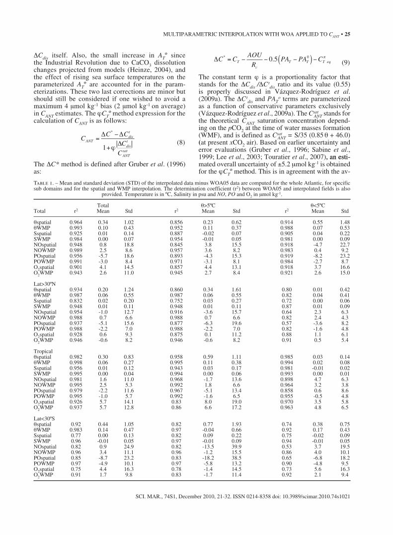
Table 1. – Mean and standard deviation (STD) of the interpolated data minus WOA05 data are computed for the whole Atlantic, for specific sub domains and for the spatial and WMP interpolation. The determination coefficient (r2) between WOA05 and interpolated fields is also

provided. Temperature is in ºC, Salinity in psu and NO, PO and O2 in µmol kg-1.

Total θ>5ºC θ<5ºC Total r2 Mean Std r2 Mean Std r2 Mean Std

θspatial 0.964 0.34 1.02 0.856 0.23 0.62 0.914 0.55 1.48θWMP 0.993 0.10 0.43 0.952 0.11 0.37 0.988 0.07 0.53Sspatial 0.925 0.01 0.14 0.887 -0.02 0.07 0.905 0.04 0.22SWMP 0.984 0.00 0.07 0.954 -0.01 0.05 0.981 0.00 0.09NOspatial 0.948 0.8 18.8 0.845 3.8 15.5 0.918 -4.7 22.7NOWMP 0.989 2.5 8.6 0.957 3.6 8.2 0.983 0.4 9.2POspatial 0.956 -5.7 18.6 0.893 -4.3 15.3 0.919 -8.2 23.2POWMP 0.991 -3.0 8.4 0.971 -3.1 8.1 0.984 -2.7 8.7O2spatial 0.901 4.1 14.5 0.857 4.4 13.1 0.918 3.7 16.6O2WMP 0.943 2.6 11.0 0.945 2.7 8.4 0.921 2.6 15.0 Lat>30ºN θspatial 0.934 0.20 1.24 0.860 0.34 1.61 0.80 0.01 0.42θWMP 0.987 0.06 0.55 0.987 0.06 0.55 0.82 0.04 0.41Sspatial 0.832 0.02 0.20 0.752 0.03 0.27 0.72 0.00 0.06SWMP 0.948 0.01 0.11 0.948 0.01 0.11 0.87 0.01 0.09NOspatial 0.954 -1.0 12.7 0.916 -3.6 15.7 0.64 2.3 6.3NOWMP 0.988 0.7 6.6 0.988 0.7 6.6 0.82 2.4 4.3POspatial 0.937 -5.1 15.6 0.877 -6.3 19.6 0.57 -3.6 8.2POWMP 0.988 -2.2 7.0 0.988 -2.2 7.0 0.82 -1.6 4.8O2spatial 0.928 0.6 9.3 0.875 0.1 11.2 0.88 1.1 6.1O2WMP 0.946 -0.6 8.2 0.946 -0.6 8.2 0.91 0.5 5.4 Tropical θspatial 0.982 0.30 0.83 0.958 0.59 1.11 0.985 0.03 0.14θWMP 0.998 0.06 0.27 0.995 0.11 0.38 0.994 0.02 0.08Sspatial 0.956 0.01 0.12 0.943 0.03 0.17 0.981 -0.01 0.02SWMP 0.995 0.00 0.04 0.994 0.00 0.06 0.993 0.00 0.01NOspatial 0.981 1.6 11.0 0.968 -1.7 13.6 0.898 4.7 6.3NOWMP 0.995 2.5 5.3 0.992 1.8 6.6 0.964 3.2 3.8POspatial 0.979 -2.2 11.6 0.967 -5.1 13.4 0.858 0.6 8.6POWMP 0.995 -1.0 5.7 0.992 -1.6 6.5 0.955 -0.5 4.8O2spatial 0.926 5.7 14.1 0.83 8.0 19.0 0.970 3.5 5.8O2WMP 0.937 5.7 12.8 0.86 6.6 17.2 0.963 4.8 6.5 Lat<30ºS θspatial 0.92 0.44 1.05 0.82 0.77 1.93 0.74 0.38 0.75θWMP 0.983 0.14 0.47 0.97 -0.04 0.66 0.92 0.17 0.43Sspatial 0.77 0.00 0.13 0.82 0.09 0.22 0.75 -0.02 0.09SWMP 0.96 -0.01 0.05 0.97 -0.01 0.09 0.94 -0.01 0.05NOspatial 0.82 0.9 24.9 0.82 -13.5 39.9 0.53 3.7 19.5NOWMP 0.96 3.4 11.1 0.96 -1.2 15.5 0.86 4.0 10.1POspatial 0.85 -8.7 23.2 0.83 -18.2 38.5 0.65 -6.8 18.2POWMP 0.97 -4.9 10.1 0.97 -5.8 13.2 0.90 -4.8 9.5O2spatial 0.75 4.4 16.3 0.78 -1.4 14.5 0.73 5.6 16.3O2WMP 0.91 1.7 9.8 0.83 -1.7 11.4 0.92 2.1 9.4



erage uncertainty of 5.6 mmol kg-1 for ΔCdis (Vázquez-Rodríguez et al., 2009a).

For the application case of CANT interpolation (var = CANT in equation 1) the computed CANT must be nor-malized to a reference year (1994) using the following expression:

CC

CCANT i

ANTsat

ANTsat year ANT i

y,

,

, ,1994

1994

= ear (10)

The reason for doing this comes from the transient tracer nature of CANT and the fact that the CARINA database spans quite a long time period. Therefore, the interpolated CANT referenced to 1994 (C1994

ANT) is com-puted as

CC f

fANT

ANT i ij

i

ij

i

1994

1994

1

1

=( )

( )∑∑ −

−

, (11)

which is valid for both CANT reconstruction methods.

RESULTS AND DISCUSSION

To assess the quality of both types of interpola-tion, their results were evaluated against the WOA05 data, i.e. the interpolated potential temperature, salin-ity, ‘NO’ and ‘PO’ obtained from equation (1) were compared with the corresponding original values from WOA05 variables. Since these parameters were involved in factor’s calculation of the WMP interpola-tion (Eqs. 2, 4), a more independent check was done by interpolating O2 and comparing it against the WOA05

O2 data. When the interpolation methods had been as-sessed, they were applied to CANT, using both jCTº and TrOCA methods, in order to get the 3D distribution and the total inventories.

The mean and standard deviation (STD) of the in-terpolated data minus the reference WOA05 data (S, θ, ‘NO’, ‘PO’ and O2) were computed for the whole domain and for specific sub-domains (Table 1). Also, the correlation between interpolated and reference fields was characterized with the determination coeffi-cient (r2). Three zones were selected depending on the general variability of water masses, namely: northern latitudes (lat >30ºN), tropical latitudes and southern latitudes (lat <30ºS). In addition, two depth levels were set with respect to the 5ºC isoterms: θ >5ºC and θ <5ºC. The 5ºC isotherm represents a coarse bound-ary between the little-ventilated deep waters and the younger, more ventilated upper and intermediate wa-ters. It also splits the CANT inventories in about half.

The climatological annual mean of WOA05 po-tential temperature along the 28ºW section in WOA05 (Fig. 1) is shown in Figure 2A. The spatially-inter-polated potential temperature (θspatial) from the CA-RINA data base is close to the WOA05 data (Fig. 2B). However, some misfits do show up when the residuals are plotted (Fig. 2D). The larger residuals are located in the upper layer, where absolute values higher than 2ºC are reached. In the deep water there is a better agreement, although southward of 40ºS there is a large thick layer holding a systematic bias, higher than 1ºC. On the other hand, the potential temperature

Fig. 1. – A, CARINA stations with available variables needed to estimate CANT and section 28ºW plotted. B, WOA05 data grid sample with θ (ºC).

A B



from the WMP interpolation (θWMP) (Fig. 2C) shows a better agreement and lower residuals than the spa-tial interpolation. This time, as for θspatial, the best fit is found in deep waters, north of 45ºS. Statistically speaking, the best fit (Table 1) is obtained by the WMP interpolation irrespective of whether the whole Atlantic is included or the interpolation is restricted to the sub-domains previously defined. The largest

differences between the two kinds of interpolation are located in the upper layer (θ >5ºC), where r2 increases noticeably when the WMP interpolation is used. More specifically, the best fits are obtained in the tropical region and northern latitudes, whereas the southern latitudes show the worst fits. This is probably due to the lower density of data that the CARINA database has in the Southern Ocean.

Fig. 2. – Potential temperature (ºC) variability along 28ºW from the WOA05 dataset (A), spatially interpolated from CARINA data (B). Residuals of WMP interpolated (C) and spatially interpolated (D) potential temperature both as interpolated minus WOA05.

Fig. 3. – Salinity variability along 28ºW from the WOA05 dataset (A), spatially interpolated from CARINA data (B). Residuals of WMP interpolated (C) and spatially interpolated (D) salinity, both as interpolated minus WOA05.

A

C

B

D

A

C

B

D



Figure 3A shows the WOA05 climatological an-nual mean of salinity along the vertical section defined by the 28ºW meridian (Fig. 1). As in the case of θspatial, the spatially interpolated salinity (Sspatial) from the CA-RINA database is quite close to the WOA05 reference data (Fig. 3B). Some misfits can be observed when the residuals between the spatially interpolated and WOA05 salinity values are plotted for the 28ºW section (Fig. 3D). For instance, there is a considerable error

located around the salinity minimum associated with the presence of Antarctic Intermediate Water (AAIW) (Mémery et al., 2000). Again, the greater residuals are found in the upper layers where absolute values higher than 0.2 psu are observed. Although in the deep waters the concordance is high in general, south of 40ºS there is still the same thick layer of large biases (higher than 0.05 psu in this case) also observed with the θspatial. The WMP interpolation of salinity (SWMP) (Fig. 3C) shows

Fig. 4. – NO (µmol kg-1) variability along 28ºW from the WOA05 dataset (A), spatially interpolated from CARINA data (B). Residuals of WMP interpolated (C) and spatially interpolated (D) NO, both as interpolated minus WOA05.

Fig. 5. – O2 (µmol kg-1) variability along 28ºW from the WOA05 dataset (A), spatially interpolated from CARINA data (B). Residuals of WMP interpolated (C) and spatially interpolated (D) O2, both as interpolated minus WOA05.

A

C

B

D

A

C

B

D



better agreement and lower residuals than the Sspatial in-terpolation in all sub-domains (Table 1), proving again a superior performance of the WMP over the purely spatial interpolation method. Generally, both interpo-lation methods seem to perform better for salinity in the deep waters north of 45ºS (Fig. 3D). Quantitatively speaking, the best fit to WOA05 values is obtained by the WMP interpolation in the tropical region (Table 1). The largest discrepancies between results from the two interpolation algorithms are found in the upper layers (θ >5ºC) of North Atlantic waters. Here, the r2 obtained with the WMP algorithm are better by far than the ones produced by the spatial approach. However, the r2

values obtained for S are generally slightly lower than those of θ.

The climatological annual mean of ‘NO’ is shown along 28ºW (Fig. 4A). Since ‘NO’ and ‘PO’ are highly correlated, the ‘PO’ fields are not shown for the sake of conciseness. The spatial interpolation of ‘NO’ (NOspa-

tial) is close to the WOA05 data (Fig. 4B), with a most noteworthy r2 of 0.948 (Table 1) for the whole Atlan-tic. The upper layers of the ocean, and particularly the Southern Ocean (SO), display the largest anomalies, which exceptionally reach offsets of 50 µmol kg-1 (Fig. 4D). In general, the NOWMP output shows better agree-ment, lower standard deviations in residuals and higher determination coefficients than the NOspatial in every subdomain (Table 1). Unlike the θ case, the best fit is found in the upper warm layers of the Atlantic Ocean rather than in the deep ones. This is likely due to the relatively high variability of ‘NO’ observed in the up-per layer. Conversely, the worst fit (lowest r2), is found in the deep layers of the Southern Ocean.

The interpolated oxygen fields can be used as a test to assess the quality of the interpolation from CARINA data, given that this variable is common to both datasets and it is not used in the interpolation algorithms. The concentration of oxygen is controlled by the biological and solubility pumps. The clima-tological annual mean of O2 along the 28ºW section (Fig. 5A) exhibits a strong minimum in the upper layer in the tropical region caused by the reminerali-zation of organic matter (biological pump predomi-nance). The high values observed in the polar areas are the consequence of the high solubility of oxygen in cold surface waters (solubility pump prevails the biological processes). The spatially interpolated O2 (O2spatial) (Fig. 5B) closely resembles the WOA05 O2 distribution along the 28ºW vertical section (Fig. 5A). It is generally well correlated (r2 of 0.90, Table 1) in the Atlantic Ocean, though the purely-spatial in-terpolation has a slight tendency to over-spline some O2 gradients in the southern latitudes. The largest differences and lowest correlations between the ob-served and the O2spatial fields are located in the up-per Atlantic layer (ranging from -25 to 20 µmol kg-1) and in the Southern Ocean, where offsets may reach up to 50 µmol kg-1 (Fig. 5D). The best fits obtained belong to the cold deep layers of the tropical region.

The O2 WMP interpolation (O2WMP) (Fig. 5C) is in better agreement with direct observations, has lower residuals (Fig. 5C) and has higher r2 in general than the spatial interpolation (r2 of 0.94 vs. r2 of 0.90 re-spectively, Table 1). Unlike for the rest of domains, in deep tropical waters the WMP interpolation seems not to perform up to its potential, as the results from the spatial interpolation appear to be more in accord-ance with the observed fields. Most importantly, the WMP interpolation algorithm yields robust estimates in the Southern Ocean, where data coverage of the CARINA database is rather sparse.

As CANT is indistinguishable from natural CO2, there are no CANT benchmarks against which the esti-mations can be compared. Figure 6 shows the spatial and WMP interpolations of CANT computed using the jCTº method. The general pattern of the distributions is similar to those given by Lee et al. (2003) and Vázquez-Rodríguez et al. (2009b). Sabine et al. (2004), using GLODAP gridded database, produced a total inventory of CANT for the Atlantic of 40 Pg-C. Previously, Lee et al. (2003) obtained a total inventory of 47 Pg-C by us-(2003) obtained a total inventory of 47 Pg-C by us- obtained a total inventory of 47 Pg-C by us-ing an ungridded GLODAP database. Using CFC data, Waugh et al. (2006) obtained a total inventory of 48 Pg-C. A comparative study using five long transoce-anic cruises was performed by Vázquez-Rodríguez et al. (2009b). They found that jCTº and TrOCA turn out 55 and 51 Pg-C respectively. The results obtained here with CARINA gridded showed the same integrated inventories as Vázquez-Rodríguez et al. (2009b) for the jCTº method, but a higher value of 58 Pg-C for the TrOCA method. The main differences from the GLODAP gridded data (Lee et al., 2003; Key et al., 2004) are located in the South Atlantic, where a large number of GLODAP estimates (obtained from the ΔC* method, Gruber et al., 1996) are negative. The GLO-DAP values of CANT for the Southern Ocean are lower than the ones computed here. This negative bias in the CANT estimates from the GLODAP dataset has been identified by several authors (Lo Monaco et al., 2005; Waugh et al., 2006; Vázquez-Rodríguez et al., 2009b)The discrepancies among the interpolation methods are rather low except in the upper layers and in the South-ern Ocean (Fig. 6C). The WMP interpolation produces higher values of CANT than the spatial method in the deep Southern Ocean (θ <5ºC) and lower values in the upper layers where biases reach about ~8 µmol kg-1. In terms of CANT inventories the discrepancies are quite low and there are systematically lower (higher) values in the upper (lower) layer when the spatial interpola-tion is used (Table 2). The estimated total inventory of jCTº CANT for the Atlantic is 55 Pg-C, independently of the interpolation method applied. Nevertheless, some minor discrepancies are found when the warm and cold water (θ above or below the 5ºC isotherm, respectively) inventories are examined separately (Table 2).

The above-described pattern is quite similar to the one obtained when the TrOCA method is used to es-timate CANT. The total inventory does not change too



much (roughly less than 5%, Table 2) when different interpolation methods are used, although the invento-ries in the warm and cold layers for the whole Atlantic Ocean are around 1.5 Pg-C different depending on the interpolation method used. Using the TrOCA method produces a slightly higher CANT inventory. The TrOCA method gives higher values in the surface layer (higher penetration) and in the deep Northern North Atlantic (Fig. 7). In comparison, the jCTº method gives slightly higher values in practically all deep water masses and in the Southern Ocean, except for the Antarctic Bottom Water (AABW). Again, the major differences found in the southern latitudes are a consequence of the low density of carbon system data in this region.

Future work will be needed to improve the inter-polation method and obtain an uncertainty assessment, and to iterate back and forth to the original data fol-lowing a Barnes schema to fine-tune the interpolation. After these improvements have been achieved and with uncertainties available, the enhanced interpola-tion method could be used to interpolate the param-eters available in CARINA and GLODAP, in order to provide an enhanced gridded product. Also, more CANT estimation techniques such as TTD and ΔC* can be incorporated and applied to the CARINA database so that their inventories will be obtained.

CONCLUSIONS

The WMP interpolation method offers improve-ments compared with a traditional spatial gridding, and even with an objective analysis spatial gridding. By using an auxiliary database (WOA05) constructed with more resolution data on bio-geochemical conservative parameters, the WMP method has more information for the gridding task than any other exclusively spatial alternative.

The total inventory of CANT (referred to 1994) for the Atlantic Ocean is estimated to be about 55-58 Pg-C depending on the CANT estimation technique ap-plied (jCTº or TrOCA, respectively). The interpolation methods used here (spatial and WMP) do not have significant effects on the estimates of CANT total inven-tories, due to compensation effects between domains. Nevertheless, there exist some minor differences in the

Table 2. – CANT inventories (Pg-C) in the Atlantic and in different latitudinal bands and layers using the TrOCA and jCTº methods.

CANT(Pg-C) 1994 jCTº TrOCA Zone θ(ºC) Spatial WMP diff Spatial WMP diff

Lat>30ºN <5 6.9 7.0 0.1 8.1 8.1 0.0Lat>30ºN ≥5 6.0 5.8 -0.2 6.7 6.5 -0.2Tropical <5 12.8 13.4 0.6 12.7 13.2 0.5Tropical ≥5 10.2 9.7 -0.5 10.5 9.9 -0.6Lat<30ºS <5 15.5 16.3 0.8 15.9 16.7 0.8Lat<30ºS ≥5 3.7 3.1 -0.6 4.0 3.2 -0.8Atlantic Ocean <5 35.2 36.7 1.4 36.6 38.0 1.4Atlantic Ocean ≥5 19.9 18.6 -1.3 21.2 19.6 -1.7

Total 55.1 55.2 0.1 57.9 57.6 -0.2

Fig. 7. – CANT (µmol kg-1) determined by the TrOCA method along 28ºW using spatial interpolation (A) and WMP interpolation (B). Residuals between the two interpolations are shown (C) as spatially

interpolated minus WMP interpolated.

Fig. 6. – CANT (µmol kg-1) determined by the jCTº method along 28ºW using spatial interpolation (A) and WMP interpolation (B). Residuals between the two interpolations are shown (C) as spatially

interpolated minus WMP interpolated.

A

C

B

A

C

B



results obtained by the different interpolation methods. The WMP interpolation method performs better than the spatial one, particularly in regions with less density of initial data (most importantly the Southern Ocean) from the CARINA dataset. Finally, the differences be-tween the interpolation methods transcend to the realm of CANT estimation above and below the 5ºC isopleth. The spatial method tends to produce lower (higher) CANT values in the water below (above) the isotherm of 5ºC than the WMP interpolation method.

ACKNOWLEDGEMENTS

We would like to extend our gratitude to the chief scientists, scientists and crew who participated and of-fered their dedication to the oceanographic cruises used in this study. This work was developed and funded by the European Commission within the 6th Framework Pro-gramme (EU FP6 CARBOOCEAN Integrated Project, Contract no. 511176), MEC (CTM2006-27116-E/MAR) and by the Xunta de Galicia within the INCITE framework (M4AO project PGIDIT07PXB402153PR)

We also wish to thank the editor and the two anony-mous reviewers, whose comments greatly contributed to improving and focusing the manuscript.

REFERENCES

Anderson, L.A. and J.L. Sarmiento. – 1994. Redfield Ratios of Remineralization Determined by Nutrient Data Analysis. Glo-bal Biogeochem. Cycles, 8: 65-80.

Antonov, J.I., R.A. Locarnini, T.P. Boyer, A.V. Mishonov, H.E. Garcia and S. Levitus. – 2006. World Ocean Atlas 2005, Vol-ume 2: Salinity. S. Levitus. NOAA Atlas NESDIS 62, U.S. Gov-ernment Printing Office, Washington, D.C.: 182.

Bennett, A.F. – 1992. Inverse methods in physical oceanography. Cambridge University Press.

Bretherton, F.P., R.E. Davis and C.B. Fandry. – 1976. A technique for objective analysis and design of oceanographic experiments applied to MODE-73. Deep-Sea Res., 23: 559-582.

Broecker, W.S. – 1974. “NO”, a conservative water-mass tracer. Earth Planet. Sci. Let., 23.

Canadell, J.G., C. Le Quéré, M.R. Raupach, C.B. Field, E.T. Buiten-huis, P. Ciais, T.J. Conway, N.P. Gillett, R.A. Houghton and G. Marland. _ 2007. Contributions to accelerating atmospheric CO2 growth from economic activity, carbon intensity, and efficiency of natural sinks. Proc. Natl. Acad. Sci., 104: 18866.

Emery, W.J. and R.E. Thomson. – 2001. Data analysis methods in physical oceanography. Elsevier Science.

Freeland, H.J. and W.J. Gould. – 1976. Objective analysis of meso-scale ocean circulation features. Deep-Sea Res., 23: 915-923.

Gandin, L.S. and R. Hardin. – 1965. Objective analysis of mete-orological fields. Israel program for scientific translations Jerusalem.

Garcia, H.E., R.A. Locarnini, T.P. Boyer, J.I. Antonov and S. Levi-tus. – 2006a. World Ocean Atlas 2005, Volume 3: Dissolved Oxygen, Apparent Oxygen Utilization, and Oxygen Saturation. S. Levitus. NOAA Atlas NESDIS 63, U.S. Government Printing Office, Washington, D.C.: 342.

Garcia, H.E., R.A. Locarnini, T.P. Boyer, J.I. Antonov and S. Levi-tus. – 2006b. World Ocean Atlas 2005, Volume 4: Nutrients (phosphate, nitrate, silicate). S. Levitus. NOAA Atlas NESDIS 64, U.S. Government Printing Office, Washington, D.C.: 396.

Gruber, N., J.L. Sarmiento and T.F. Stocker. – 1996. An improved method for detecting anthropogenic CO2 in the oceans. Global Biogeochem. Cycles, 10: 809-837.

Hedges, J.I., W.A. Clark and G.L. Cowie. – 1988. Organic mat-ter sources to the water column and superficial sediments of a

marine bay. Limnol. Oceanogr., 33: 1116-1136.Heinze, C. _ 2004. Simulating oceanic CaCO3 export production in

the greenhouse. Geophys. Res. Lett, 31: L16308.Hoppema, M., A. Velo, S. van Heuven, T. Tanhua, R.M. Key, X.

Lin, D.C.E. Bakker, F.F. Pérez, A.F. Ríos, C. Lo Monaco, C.L. Sabine, M. Álvarez and R.G.J. Bellerby. – 2009. Consistency of cruise data of the CARINA database in the Atlantic sector of the Southern Ocean. Earth Syst. Sci. Data, 1: 63-75.

Jalickee, J.B. and D.R. Hamilton. – 1977. Objective analysis and classification of oceanographic data. Tellus, 29.

Joos, F., G.K. Plattner, T.F. Stocker, O. Marchal and A. Schmittner. – 1999. Global warming and marine carbon cycle feedbacks on future atmospheric CO2. Science, 284: 464.

Key, R.M., A. Kozyr, C.L. Sabine, K. Lee, R. Wanninkhof, J.L. Bullister, R.A. Feely, F.J. Millero, C. Mordy and T.H. Peng. _ 2004. A global ocean carbon climatology: Results from Global Data Analysis Project (GLODAP). Global Biogeochem. Cycles, 18, GB4031.

Key, R.M., T. Tanhua, A. Olsen, M. Hoppema, S. Jutterström, C. Schir-nick, S. van Heuven, A. Kozyr, X. Lin, A. Velo, D.W.R. Wallace and L. Mintrop. – 2010. The CARINA data synthesis project: In-troduction and overview. Earth Syst. Sci. Data, 2: 105-121.

Kortzinger, A., J.I. Hedges and P.D. Quay. – 2001. Redfield ratios revisited: Removing the biasing effect of anthropogenic CO2. Limnol. Oceanogr., 964-970.

Le Quéré, C., C. Rodenbeck, E.T. Buitenhuis, T.J. Conway, R. Langenfelds, A. Gomez, C. Labuschagne, M. Ramonet, T. Na-kazawa and N. Metzl. – 2007. Saturation of the Southern Ocean CO2 sink due to recent climate change. Science, 316: 1735.

Lee, K., S.D. Choi, G.H. Park, R. Wanninkhof, T.H. Peng, R.M. Key, C.L. Sabine, R.A. Feely, J.L. Bullister and F.J. Millero. – 2003. An updated anthropogenic CO2 inventory in the Atlantic Ocean. Global Biogeochem. Cycles, 17: 1116.

Lo Monaco, C., C. Goyet, N. Metzl, A. Poisson and F. Touratier. – 2005. Distribution and inventory of anthropogenic CO2 in the Southern Ocean: Comparison of three data-based methods. J. Geophys. Res, 110: 9.

Locarnini, R.A., A.V. Mishonov, J.I. Antonov, T.P. Boyer, H.E. Garcia and S. Levitus. – 2006. World Ocean Atlas 2005, Vol-ume 1: Temperature. S. Levitus. NOAA Atlas NESDIS 61, U.S. Government Printing Office, Washington, D.C.: 182.

Matear, R.J., C.S. Wong and L. Xie. – 2003. Can CFCs be used to determine anthropogenic CO2? Global Biogeochem. Cycles, 17: 1013.

Mémery, L., M. Arhan, X.A. Alvarez-Salgado, M.J. Messias, H. Mercier, C.G. Castro and A.F. Ríos. – 2000. The water masses along the western boundary of the south and equatorial Atlantic. Progr. Oceanogr., 47: 69-98.

Pérez, F.F., C. Mourino, F. Fraga and A.F. Ríos. – 1993. Displace-ment of water masses and remineralization rates off the Iberian Peninsula by nutrient anomalies. J. Mar. Res., 51: 869-892.

Ríos, A.F., F. Fraga and F.F. Pérez. – 1989. Estimation of coef-ficients for the calculation of “NO”, “PO” and “CO”, starting from the elemental composition of natural phytoplankton. Sci. Mar., 53: 779-784.

Sabine, C.L., R.M. Key, K.M. Johnson, F.J. Millero, A. Poisson, J.L. Sarmiento, D.W.R. Wallace and C.D. Winn. – 1999. An-thropogenic CO2 inventory of the Indian Ocean. Global Biogeo-chem. Cycles, 13: 179-198.

Sabine, C.L., R.A. Feely, N. Gruber, R.M. Key, K. Lee, J.L. Bul-lister, R. Wanninkhof, C.S. Wong, D.W.R. Wallace and B. Tilbrook. – 2004. The oceanic sink for anthropogenic CO2. Sci-ence, 305: 367-371.

Tanhua, T., A. Olsen, M. Hoppema, S. Jutterström, C. Schirnick, S. Van Heuven, A. Velo, X. Lin, A. Kozyr, M. Alvarez, D.C.E. Bakker, P. Brown, E. Falck, E. Jeansson, C. Lo Monaco, J. Olaf-sson, F.F. Perez, D. Pierrot, A.F. Rios, C.L. Sabine, U. Schuster, R. Steinfeldt, I. Stendardo, L.G. Anderson, N.R. Bates, R.G.J. Bellerby, J. Blindheim, J.L. Bullister, N. Gruber, M. Ishii, T. Johannessen, E.P. Jones, J. Köhler, A. Körtzinger, N. Metzl, A. Murata, S. Musielewicz, A.M. Omar, K.A. Olsson, M. de la Paz, B. Pfeil, F. Rey, M. Rhein, I. Skjelvan, B. Tilbrook, R. Wanninkhof, L. Mintrop, D.W.R. Wallace and R.M. Key. – 2009. CARINA Data Synthesis Project. ORNL/CDIAC-157, NDP-091, Carbon Dioxide Information Analysis Center, Oak Ridge National Laboratory, U.S. Departament of Energy, Oak Ridge, Tennessee, 37831-6335.



Tanhua, T., R. Steinfeldt, R.M. Key, P. Brown, N. Gruber, R. Wan-ninkhof, F.F. Pérez, A. Körtzinger, A. Velo, U. Schuster, S. van Heuven, J.L. Bullister, I. Stendardo, M. Hoppema, A. Olsen, A. Kozyr, D. Pierrot, C. Schirnick and D.W.R. Wallace. – 2010. Atlantic Ocean CARINA data: overview and salinity adjust-ments. Earth Syst. Sci. Data, 2: 17-34.

Thomas, H. and V. Ittekkot. – 2001. Determination of anthropo-genic CO2 in the North Atlantic Ocean using water mass ages and CO2 equilibrium chemistry. J. Mar. Syst., 27: 325-336.

Touratier, F., L. Azouzi and C. Goyet. – 2007. CFC-11, Δ14C and 3H tracers as a means to assess anthropogenic CO2 concentra-tions in the ocean. Tellus B, 59: 318-325.

U.S. Department of Commerce, N.O.a.A.A., National Geophysi-cal Data Center. – 2006. 2-minute Gridded Global Relief Data (ETOPO2v2).

Vázquez-Rodríguez, M., X.A. Padin, A.F. Ríos, R.G.J. Bellerby and F.F. Pérez. – 2009a. An upgraded carbon-based method to esti-mate the anthropogenic fraction of dissolved CO2 in the Atlantic Ocean. Biogeosci. Discuss., 6: 4527-4571.

Vázquez-Rodríguez, M., F. Touratier, C. Lo Monaco, D.W. Waugh, X.A. Padin, R.G.J. Bellerby, C. Goyet, N. Metzl, A.F. Ríos and F.F. Pérez. – 2009b. Anthropogenic carbon distributions in the Atlantic Ocean: data-based estimates from the Arctic to the Antarctic. Biogeosciences, 6: 439-451.

Waugh, D.W., T.M. Hall, B.I. McNeil, R. Key and R.J. Matear. – 2006. Anthropogenic CO2 in the oceans estimated using transit time distributions. Tellus B, 58: 376-389.

Received November 1, 2008. Accepted July 26, 2010.Published online November 13, 2010.

Documents

A multiparametric method of interpolation using …digital.csic.es/bitstream/10261/33619/1/A.Velo.pdf · en el Atlántico, calculado por dos métodos de estimación sobre la base