Page - 1 - of 12

Land Suitability Analysis for Agricultural Crops using Multi-Criteria Decision Making and GIS Approach

Dr Kuldeep Pareta* and Dr C. K. Jain**

*Project Manager (RS, GIS, and NRM), Spatial Decisions, B-30 Kailash Colony, New Delhi - 48

**Senior Lecture, Department of General and Applied Geography, Dr H.S.G. University, Sagar (M. P.)

Corresponding author: kuldeep.p@spatialdecisions.in

Keywords: Land Suitability Analysis, Landuse-Landcover, Multi-Criteria Decision Making Approach, Remote Sensing & GIS

Abstract:

Crop-land suitability analysis is a prerequisite to achieve optimum utilization of the available land resources for

sustainable agricultural production. One of the most important and urgent problems in the study area is to improve

agricultural land management and cropping patterns to increase the agricultural production with efficient use of land

resources. In Vattanam, and Kaliyanagari village, Tiruvadanai taluck of Ramanathapuram district, agriculture is the

mainstay of economy and crop land is the most important but the production is very low. In particular the crop

production of study area does not meet the demands due to its rapidly growing population. The aim of this study is to

determine physical land suitability for crop using a Multi-Criteria Evaluation (MCE) and GIS approach and to compare

present land use vs. potential land use. The aim in integrating Multi-Criteria Evaluation with Geographical Information

Systems (GIS) is to provide more flexible and more accurate decisions to the decision makers in order to evaluate the

effective factors.

The study was carried out in Vattanam, and Kaliyanagari village, Tiruvadanai taluck in the north of Ramanathapuram

district of Tamilnadu state. Relevant biophysical variables of landuse, soil, climatic, and topography were considered for

suitability analysis. All data were stored in ArcGIS 9.3.1 environment and the factor maps were generated. For Multi-

Criteria Evaluation (MCE), Pairwise Comparison Matrix known as Analytical Hierarchy Process (AHP) was applied and the

suitable areas for crop land were identified. To generate present land use/cover map, QuickBird (60 cm) 16 April, 2010,

and IRS-P6, Resourcesat-1 LISS-IV Mx (5.8m) 26 September, 2009 satellite image was classified using ERDAS Imagine 9.3

by means of supervised classification.

According to the present land use/cover map, the agricultural land was 446.35 hectare (29.47%). Finally, we overlaid the

land use/cover map with the suitability map for crop production to identify differences and similarities between the

present and potential land use. However, the crop-land evaluation results of the present study identified that in the study

area, 32.10 percent of total land being used was under highly suitable areas and 56.17 percent was under moderately

suitable areas. The results showed that agricultural practiced, which prevailed in the study area didn’t match with the

potential suitability in the marginally suitable area. Thus, the average yield of the study area was substantially affected

because of a significant proportion of crop land was under marginally suitable areas. This research provided information

at local level that could be used by farmers to select crop land, cropping patterns and suitability.

1.0 - Introduction:

Agriculture, being the most primitive occupation of the civilized man, draws much on its development starting from

shifting cultivation to advanced precision farming. With the advancement in the civilization man came to know about

more crops and started to cultivate many crops (Chen & Hwang 1992)1. Population increase and advancement in the

civilization made man to settle at one place and to cultivate the same area year after year. Now agriculture became a

profession is given the name commercial agriculture, and precision agriculture and sustainable agriculture as being the part

of it. Nowadays, the population of the planet is growing dramatically. In order to meet the increasing demand for the food

the farming community has to produce more and more. Under present situations, where the land is a limiting factor, it is

impossible to bring more area under cultivation, so farming community should tackle this challenge of producing more

and more food with the available land only. On the contrary, the increasing global concern to-wards the health of

mankind and environment protests the use of higher amount of pesticides and fertilizers, genetically manipulated plants

Page - 2 - of 12

etc. However, latter are the current technologies having the potentiality to increase the food production. To overcome this

concern the farming community has to produce more and more, high quality food using eco-friendly practices. This

need for eco-friendly practices have paved the way for the concepts like precision farming, sustainable farming,

organic farming etc. Higher productivity, profitability and health of mankind as well as environment are the concerns

of the present agriculture. Hence much attention is shifted on selection of a crop, which suits an area the best.

This suitability is a function of crop requirements, soil and land characteristics. Matching the land characteristics with the

crop requirements gives the suitability. So, ‘Suitability is a measure of how well the qualities of a land unit match the

requirements of a particular form of land use' (Saouma, 1986)2. Besides the land / soil characteristics socio-economic,

market and infrastructure characteristics are the other driving forces that can influence the crop selection. To develop the

multi-criteria decision making technique using remote sensing and GIS for land suitability analysis for agricultural crops is

the main object of this study.

1.1 - Problem:

Land suitability is the ability of a given type of land to support a defined use. The process of land suitability classification is

the evaluation and grouping of specific areas of land in terms of their suitability for a defined use (Sharifi & Herwijinen,

2003)3. The main objective of the land evaluation is the prediction of the natural capacity of a land unit to support a

specific land use for a long period of time without deterioration, in order to minimize the socio-economic and

environmental costs. Land suitability analysis is an interdisciplinary approach by including the information from different

domains like soil science, crop science, meteorology, social science, economics and management.

1.2 - Need for Multi Criteria Decision Making:

Agricultural land suitability is an interdisciplinary approach. Determination of optimum land use type for an area involves

integration of data from various domains and sources like soil science to social science, meteorology to management

science. All these major streams can be considered as separate groups; further each group can have various

parameters (criteria) in itself. However all the criteria are not equally important, every criterion will contribute towards

the suitability at different degrees (Gundimeda, 2007)4. The relative degree of contribution of various criteria can be

addressed well when they are grouped into various groups and organized at various hierarchies. Agricultural land

suitability also involves major decisions at various levels starting from choosing a major land use types, selection of

criteria, organization of the criteria, deciding suitability limits for each class of the criteria, deciding the preferences

(qualitative and quantitative). Relative importance of these parameters can be well evaluated to determine the

suitability by multi-criteria evaluation techniques (Nagasawa & Delowar, 2005)5.

1.3 - Role of GIS and Remote Sensing:

GIS is the tool for input, storage and retrieval, manipulation and analysis, and out put of spatial data. GIS functionality can

play a major role in spatial decision-making. Considerable effort is involved in information collection for the suitability

analysis for crop production (Eldrandaly, 2007)6. This information should present both opportunities and constraints for

the decision maker. GIS have the ability to perform numerous tasks utilizing both spatial and attribute data stored

in it. It has the ability to integrate variety of geographic technologies like GPS, Remote Sensing etc. The ultimate aim of

GIS is to provide support for spatial decisions making process. In multi-criteria evaluation many data layers are to be

handled in order to arrive at the suitability, which can be achieved conveniently using GIS. Remote sensing provides the

information about the various spatial criteria / factors under consideration. Remote sensing can provide us the

information like land use and land cover, drainage density, topography etc. (Das, 2000)7. Many of the non-spatial

parameters can also be inferred by looking at the various spatial parameters. Remote sensing in combination with GIS

will be a powerful tool to integrate and interpret real word situation in most realistic and transparent way.

2.0 - Study Area:

The study area with an extent of 1510.30 hectares is distributed in Vattanam, and Kaliyanagari village, Tiruvadanai taluck

of Ramanathapuram district, Tamilnadu. It lies between 79°2'18.69"E to 79°5'47.18"E longitude and 9°46'26.77"N to

9°50'10.34"N latitude. The study area is described in Survey of India (SOI) toposheets 58 O / 01. The area is semi dry and

Page - 3 - of 12

the rainfall is scanty with a mean annual precipitation of 827 mm. Most of the annual rainfall is received within the period

of June to September. The average annual temperature is 290 C (Max. 37.8

0C and Min. 22.3

0 C). The slope of the study

area ranges from 1 to 3% and elevation varies from sea level to 150 m above mean sea level.

Figure - 1: Location Map of the Study Area: Vattanam, and Kaliyanagari Village of Ramanathapuram District in Tamilnadu

3.0 - Data Used and Sources:

The most common date for land use and agricultural crop analysis are satellite data. They become very popular in recent

years because of their better spatial and spectral resolution and their capacity to generate multi-temporal products more

cheaply than aerial photos. Besides that land suitability analysis needs thematic maps such as soil, slope, geology, ground

water and rainfall maps. Data on crop rotation and agricultural statistics are also valuable background information. The

following data were used in this study.

Table - 1: Data Used and Sources

S. No. Input Data Layer Sources

1. Base Map Survey of India Toposheets (1:50,000 and 1:250,000 Scale) Various Satellite Imagery Other Related Maps

2. Land Use and Land Cover Map

DigitalGlobe QuickBird Satellite Imagery (60 cm Spatial Resolution) IRS - P6 (Resourcesat - 1) LISS-IV Mx Satellite Imagery (5.8 m) IRS - 1D PAN Satellite Imagery (5.8 m Spatial Resolution) IRS - P6 (Resourcesat - 1) LISS - III Satellite Imagery (23.5 m Spatial Resolution) LANDSAT - 7 ETM+ Satellite Imagery (30 m Spatial Resolution)

3. NDVI IRS - P6 (Resourcesat - 1) LISS-IV Mx Satellite Imagery (5.8 m) 4. Elevation Map Survey of India Toposheets

ASTER - DEM (30 m Spatial Resolution) & SRTM - DEM (90 m Spatial Resolution) 5. Soil Map National Bureau of Soil Survey (NBSS)

Department of Agriculture, Tamil Nadu Soil Map updated through Multi-Spectral Satellite Imagery

6. Geological Map Geological Survey of India Geological Map updated through Multi-Spectral Imagery

7. Ground Water Map

Tamilnadu Water Supply and Drainage Board, Tamil Nadu Thiessen polygons are construct by connecting a series of dug well point using

ArcGIS - 9.3.1 Software 8. Village Cadastral

Map Survey and Land Records Department Updated through Various Satellite Imagery

9. Demographic Map Census Data - 2001 District NIC Data - 2009

4.0 - Methodology:

4.1 - Spatial Multi-Criteria Decision Making:

Spatial multi-criteria decision-making is a process where geographical data is combined and transformed into a decision.

Multi-criteria decision-making involves input data, the decision maker’s preferences and manipulation of both

Page - 4 - of 12

information using specified decision rules. In spatial multi-criteria decision-making, the input data is geographical data.

Spatial multi-criteria decision-making is more complex and difficult in contrast to conventional multi-criteria decision-

making, as large numbers of factors need to be identified and considered, with high correlated relationships among

the factors (Drobne, & Lisec, 2009)8. Spatial multi-criteria decision-making aims to achieve solutions for spatial decision

problems, derived from multiple criteria (Changa, N. B., Parvathinathanb, G. & Breedenc, J. B.)9. These criteria, also called

attribute must be identified carefully to arrive at the objectives and final goal. The performance of an objective is

measured with the help of these attributes. These objectives and underlying attributes form a hierarchical structure of

evaluation criteria for a particular decision problem. These evaluation criteria should be comprehensive and measurable.

In a hierarchy, a set of criteria should be decomposable, non-redundant, complete, minimal, and computational

(Makropoulos, & Butler, 2004)10

. Further, a map layer in the GIS represents each criterion in the hierarchy (Figure: 9).

Most creative task in the decision-making is deciding what factors to include in the hierarchy structure. The

hierarchy serves two purposes; 1 - it provides the overall view of the complex relationships in the situation and 2 - it

allows decision makers to assess whether they are comparing the issues of same order or magnitude (Saaty, 1980)11

.

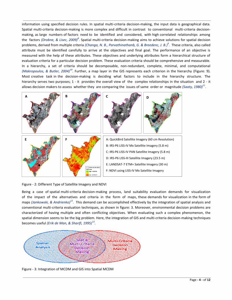
Figure - 2: Different Type of Satellite Imagery and NDVI

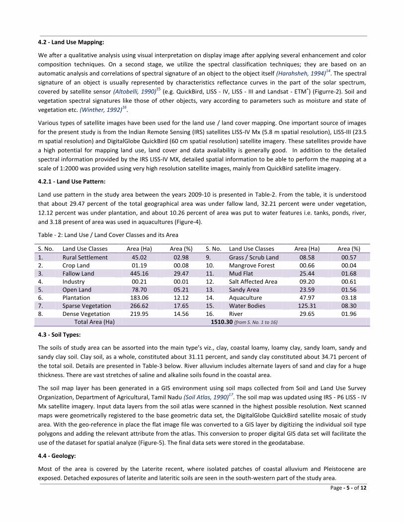
Being a case of spatial multi-criteria decision-making process, land suitability evaluation demands for visualization

of the impact of the alternatives and criteria in the form of maps, these demands for visualization in the form of

maps (Jankowski, & Andrienko)12

. This demand can be accomplished effectively by the integration of spatial analysis and

conventional multi-criteria evaluation techniques, as shown in figure: 3. Moreover, environmental decision problems are

characterized of having multiple and often conflicting objectives. When evaluating such a complex phenomenon, the

spatial dimension seems to be the big problem. Here, the integration of GIS and multi-criteria decision-making techniques

becomes useful (Erik de Man, & Sharifi, 1995)13

.

Figure - 3: Integration of MCDM and GIS into Spatial MCDM

A B C D

E F A: QuickBird Satellite Imagery (60 cm Resolution)

B: IRS-P6 LISS-IV Mx Satellite Imagery (5.8 m)

C: IRS-P6 LISS-IV PAN Satellite Imagery (5.8 m)

D: IRS-P6 LISS-III Satellite Imagery (23.5 m)

E: LANDSAT-7 ETM+ Satellite Imagery (30 m)

F: NDVI using LISS-IV Mx Satellite Imagery

Page - 5 - of 12

4.2 - Land Use Mapping:

We after a qualitative analysis using visual interpretation on display image after applying several enhancement and color

composition techniques. On a second stage, we utilize the spectral classification techniques; they are based on an

automatic analysis and correlations of spectral signature of an object to the object itself (Harahsheh, 1994)14

. The spectral

signature of an object is usually represented by characteristics reflectance curves in the part of the solar spectrum,

covered by satellite sensor (Altobelli, 1990)15

(e.g. QuickBird, LISS - IV, LISS - III and Landsat - ETM+) (Figurre-2). Soil and

vegetation spectral signatures like those of other objects, vary according to parameters such as moisture and state of

vegetation etc. (Winther, 1992)16

.

Various types of satellite images have been used for the land use / land cover mapping. One important source of images

for the present study is from the Indian Remote Sensing (IRS) satellites LISS-IV Mx (5.8 m spatial resolution), LISS-III (23.5

m spatial resolution) and DigitalGlobe QuickBird (60 cm spatial resolution) satellite imagery. These satellites provide have

a high potential for mapping land use, land cover and data availability is generally good. In addition to the detailed

spectral information provided by the IRS LISS-IV MX, detailed spatial information to be able to perform the mapping at a

scale of 1:2000 was provided using very high resolution satellite images, mainly from QuickBird satellite imagery.

4.2.1 - Land Use Pattern:

Land use pattern in the study area between the years 2009-10 is presented in Table-2. From the table, it is understood

that about 29.47 percent of the total geographical area was under fallow land, 32.21 percent were under vegetation,

12.12 percent was under plantation, and about 10.26 percent of area was put to water features i.e. tanks, ponds, river,

and 3.18 present of area was used in aquacultures (Figure-4).

Table - 2: Land Use / Land Cover Classes and its Area

S. No. Land Use Classes Area (Ha) Area (%) S. No. Land Use Classes Area (Ha) Area (%)

1. Rural Settlement 45.02 02.98 9. Grass / Scrub Land 08.58 00.57 2. Crop Land 01.19 00.08 10. Mangrove Forest 00.66 00.04 3. Fallow Land 445.16 29.47 11. Mud Flat 25.44 01.68 4. Industry 00.21 00.01 12. Salt Affected Area 09.20 00.61 5. Open Land 78.70 05.21 13. Sandy Area 23.59 01.56 6. Plantation 183.06 12.12 14. Aquaculture 47.97 03.18 7. Sparse Vegetation 266.62 17.65 15. Water Bodies 125.31 08.30 8. Dense Vegetation 219.95 14.56 16. River 29.65 01.96

Total Area (Ha) 1510.30 (from S. No. 1 to 16)

4.3 - Soil Types:

The soils of study area can be assorted into the main type’s viz., clay, coastal loamy, loamy clay, sandy loam, sandy and

sandy clay soil. Clay soil, as a whole, constituted about 31.11 percent, and sandy clay constituted about 34.71 percent of

the total soil. Details are presented in Table-3 below. River alluvium includes alternate layers of sand and clay for a huge

thickness. There are vast stretches of saline and alkaline soils found in the coastal area.

The soil map layer has been generated in a GIS environment using soil maps collected from Soil and Land Use Survey

Organization, Department of Agricultural, Tamil Nadu (Soil Atlas, 1990)17

. The soil map was updated using IRS - P6 LISS - IV

Mx satellite imagery. Input data layers from the soil atlas were scanned in the highest possible resolution. Next scanned

maps were geometrically registered to the base geometric data set, the DigitalGlobe QuickBird satellite mosaic of study

area. With the geo-reference in place the flat image file was converted to a GIS layer by digitizing the individual soil type

polygons and adding the relevant attribute from the atlas. This conversion to proper digital GIS data set will facilitate the

use of the dataset for spatial analyze (Figure-5). The final data sets were stored in the geodatabase.

4.4 - Geology:

Most of the area is covered by the Laterite recent, where isolated patches of coastal alluvium and Pleistocene are

exposed. Detached exposures of laterite and lateritic soils are seen in the south-western part of the study area.

Page 6 of 12

(Source: Somasundaram, Natarajan, Mathan and Arun Kumar - 2000)18

Table - 3: Soil Types and its Physical and Chemical Properties

S. No.

Soil Type Clay Course Loamy Loamy Clay Sand Loamy Sandy Sandy Clay Water Features Parameter

1. Soil Series Purakudikada Mettupatti Periyanayagipuram Mettupatti Kamakshipuram Madathupatti - 2. Soil Taxonomy Fine loamy,

mixed, isohyperthemic, vertic Ustorpepts

Coarse loamy, mixed, isohyperthemic, Typic Ustropepts

Fine loamy, mixed, isohyperthemic, vertic Ustorpepts

Coarse loamy, mixed, isohyperthemic, Typic Ustropepts

Fine loamy, mixed, isohyperthemic, Ultic Ustorpepts

Fine, mixed, isohyperthemic, vertic Ustorpepts

-

3. Sub-strata Type C CL LC SL S SC - 4. Modifiers dikb dm Kb dm dkm Kb - 5. Slope (%) 1 - 3 0 - 1 0 - 1 0 - 1 0 - 1 0 - 1 - 6. Fertility Capability

Unit Cdikb (1-3%) CLdm (0 - 1%) LCkb (0 - 1%) CLdm (0 - 1%) Sdkm (0 - 1%) SCkb (0 - 1%) -

7. Soil Depth (cm) 0 - 28 28 - 109

0 - 15 15 - 34

0 - 20 20 - 46

0 - 15 15 - 34

0 - 18 18 - 74

0 - 14 14 - 23

-

8. Soil Color (Dry) 2.5 YR 4/6 7.5 YR 5/6

10 YR 5/4 10 YR 5/4

10 YR 4/4 10 YR 5/6

10 YR 5/4 10 YR 5/4

10 YR 6/1 10 YR 6/6

10 YR 5/4 10 YR 4/4

-

9. Clay (%) 33.21 34.11

31.26 12.31

15.23 33.41

31.26 12.31

5.15 8.29

6.06 8.93

-

10. Texture c c

sc sl

l c

sc sl

s ls

ls ls

-

11. pH (1:2) 7.40 8.30

6.50 6.80

7.70 8.20

6.50 6.80

6.50 6.50

7.10 7.60

-

12. CEC [c mol (p+) /

kg] 21.20 24.40

18.50 16.50

17.40 16.30

18.50 16.50

15.10 17.30

16.70 15.80

-

Exchangeable Cations 13. Ca

2+ 7.0

5.5 7.0 5.0

6.5 5.0

7.0 5.0

4.0 6.0

6.0 4.0

-

14. Mg 2+

3.5 3.0

2.0 5.0

2.25 2.0

2.0 5.0

2.0 4.5

3.0 3.0

-

15. K -2

0.19 0.11

0.25 0.26

0.12 0.10

0.25 0.26

0.0 0.0

0.1 0.1

-

Total Area 16. In Hectare 469.83 112.56 177.33 23.59 47.81 524.24 154.94 17. In Percent 31.11 7.45 11.74 1.56 3.17 34.71 10.26

Page - 7 - of 12

A major part of the study area is covered with the fluvial, fuvio-marine, Aeolian and marine sediments of Quaternary age.

The fluvial deposits which are made up of sand, silt and clay in varying degrees of admixture occur along the active

channels of rivers. They have been categorized into levee, flood basin, channel bar/ point bar and paleo-channel deposits.

The paleo channel deposits comprise brown coloured, fine to medium sands with well-preserved cross-beddings.

The geo-referenced satellite digital data was used to carry out ‘on-screen’ vectorization of geological parameters.

Basically two vector layers were generated in (Figure-6). The first vector consists of geomorphic attributes and the second

vector consists of broad lithological map. In the case of image processing, spatial and spectral domain enhancement was

carried out using Earth Resource Data Analysis System (ERDAS) Imagine 9.3 software (Pareta, 2010)19

. The available IRS

LISS-III and LISS-IV Mx satellites image were used for detail assessments.

Table - 4: Lithology Types and its Area

S. No. Lithology Type Area (Ha) Area (%) S. No. Lithology Type Area (Ha) Area (%)

1 Alluvium 421.46 27.91 4 Sand 23.59 01.56 2 Laterite Recent 703.10 46.55 5 Ponds and Tanks 125.31 08.30 3 Pleistocene 207.19 13.72 6 River 29.65 01.96

Total Area (Ha) 1510.30 (from S. No. 1 to 6)

4.5 - Ground Water:

Geo-hydrologically, the study area has been divided into three zones with reference to laterite, flood basin and coastal

plain areas respectively. The North-western part of the study area exposes isolated patches of Archaeans crystallines and

Cuddalore sandstone capped by laterite / lateritic soil. The yields of bore wells of 60 to 90 m depth in the crystallines vary

from 3 to 400 lpm draw down of 10 to 12m water head. The saline aquifers in coastal tracts occur to a depth range of 80m

from ground level followed by fresh water aquifers. The quality of groundwater varies from alkaline to high saline types in

the study area (Figure-7).

In most places, ground water available at a depth beyond 2 to 3 m is saline. The fresh water available within 4 to 7 m

depths dries up quickly within 2 to 3 months after monsoon. There is acute drinking water shortage in most part of the

year.

Table - 5: Ground Water and its Area

S. No. Ground Water DTWL (m) Area (Ha)

Area (%) S. No. Ground Water DTWL (m)

Area (Ha)

Area (%)

1 0 – 1 58.62 03.88 6 5 – 6 108.09 07.16 2 1 – 2 181.84 12.04 7 6 – 7 45.00 02.98 3 2 – 3 539.00 35.69 8 7 – 8 18.61 01.23 4 3 – 4 139.48 09.24 9 More than 8 05.64 00.37 5 4 – 5 414.01 27.41 Total Area (Ha) 1510.30 (from S. No. 1 to 9)

Figure: 4 - Land use / Land Cover, 5 - Soil Data, 6 - Geology, and 7 - Ground Water

Fig. 4 Fig. 5 Fig. 6 Fig. 7

Page - 8 - of 12

4.6 - Topography of the Study Area:

Slope, aspect, and hill-shade maps of the study area were generated using ASTER DEM data with 30 spatial resolutions.

Figure - 8: Topographic Map: A - ASTER - DEM (30 m), B - Slope (in Degree), C - Slope Aspect Map, and D - Hill shade Map

5.0 - Results and Discussion:

From the seven major LUTs selected for the study area, crop land is considered to explore the ability of three multi-

criteria evaluation techniques under investigation (Samranponga, Ekasingha, & Ekasingh, 2009)20

. Evaluation criteria are

framed and organized in a hierarchy, as shown in Figure-9. Discussions with relevant experts, literature survey and

fieldwork are the major tools aided in deciding upon the LUTs, the evaluation criteria and their hierarchical

structuring. First, each criterion is categorized into seven to three suitability classes, derived from agricultural crop land

requirements. Second, land suitability evaluation is executed by three multi-criteria evaluation techniques (Yu, Chen, &

Wu 2009)21

. The results of these approaches are put together and discussed here.

5.1 - Selection of the Evaluation Criteria:

Evaluation criteria, objectives and attributes, should be identified with respect to the problem situation. A set of criteria

selected should adequately represent the decision-making environment and must contribute towards the final goal

(Omann, 2000)22

. It is known that set of attributes or criteria depends upon the system that is being analyzed. The

following evaluation criteria are considered to address the land suitability decision making.

1. Landuse: Crop Land, Fallow Land, Open Land, Plantation, Sparse / Dense Vegetation, Grass and Scrub Land

2. Soil: Soil Type, pH, Texture, Soil Depth, Fertility Capability, and Drainage

3. Lithology Type: Alluvium, Laterite Recent, and Pleistocene

4. Ground Water: Canals, Drainage, and Depth to Water Level

5. Topography: Slope, Aspect, and Hill-shade

6. Climate: Temperature, Rainfall, and Humidity

7. Infrastructure: Roads, Railways, and Market Location

5.2 - Hierarchical Organization of the Criteria:

Malczewiski (1999)23

states that relationship between the objectives and attributes has a hierarchical structure. At the

highest level one can distinguish the objectives and at lower levels, the attributes can be decomposed. Figure: 9 shows

the hierarchical structure used in this study.

5.3 - Assessing the Weights (Obtaining Decision Rules):

At higher levels of the hierarchy the criteria are required to be evaluated to derive the weights. Here the criteria

weights need to be summed up to 1, so the well-established geometric mean method is used. In this approach all the

elements in the row are multiplied and the nth root is calculated and are divided by their sum to get the normalized

weights

5.4 - Land Suitability Analysis:

Using the methodology and the data layers described above, land suitability mapping was performed for the study area.

The final suitability map has been displayed in a gradation of red to green. The green patches represent the most suitable

A B C D

Page - 9 - of 12

land for agricultural crop while the red patches denote the least. The more suitable areas are the ones which have got an

aggregate weight close to 10.

Figure - 9: Hierarchical Organization of the Criteria Considered for the Study

Table - 6: Land Suitability Classes and its Area

S. No. Land Suitability Classes Area (Ha) Area (%) S. No. Land Suitability Classes Area (Ha) Area (%)

1. Class – 01 00.27 00.02 6. Class – 06 72.12 04.78 2. Class – 02 00.62 00.04 7. Class – 07 305.06 20.20 3. Class – 03 39.67 02.63 8. Class – 08 471.16 31.20 4. Class – 04 86.27 05.71 9. Class – 09 376.09 24.90 5. Class – 05 50.37 03.33 10. Class – 10 108.67 07.20

Total Area (Ha) 1510.30 (From S. No. 1 to 10)

5.5 - Overlay Present Land Use/ Land Cover and the Suitability Map:

The present land use/land cover map and the suitability map for crop land were overlaid to identify differences as well as

similarities between the present land use and the potential land use. For crop land, a cross table between the map of

suitable areas and the land use/land cover map was obtained. In this way, we obtained useful information concerning the

Page - 10 - of 12

spatial distribution of different suitability levels, according to satellite information. This phase allowed us to fine-tune our

results, because the resultant layer provided the information about how the crop land was distributed across the various

land suitability zones.

Figure - 10: Overlay Selected Land Use/ Land Cover and the Suitability Map

6.0 - Conclusions:

Land suitability evaluation is being carried out without considering the uncertainty in the in-put data, expert knowledge.

The land suitability evaluation involves the criteria, which are in different scales ranging from nominal to ratio. Many

inputs into the GIS based land suitability evaluation are the maps of the criteria, which are representing the complex,

continuous and uncertain information in a simple, classified map with the crisp boundaries among them. The remote

sensing and GIS based methodologies and other simple techniques are used for the land suitability evaluation, which

aggravate outputs of the evaluation.

In this study, we applied remote sensing (RS) and GIS techniques to identify suitable areas for crop land. The results

obtained from this study indicate that the integration of RS-GIS and application of Multi-Criteria Evaluation using AHP

(Analytical Hierarchy Process) could provide a superior database and guide map for decision makers considering crop land

substitution in order to achieve better agricultural production. The study clearly brought out the spatial distribution of

crop land derived from Remote Sensing data in conjunction with evaluation of biophysical variables of soil, geological,

climatic, and topographic information in GIS context is helpful in crop land management options for intensification or

diversification.

This investigation is a biophysical evaluation that provides information at a local level that could be used by farmers to

select their crop land. Additionally, the results of this study could be useful for other investigators who could use these

results for diverse studies. This study has been done considering current land use/land cover, topography and soil

properties that affected the suitability classification of land use types. Therefore, it gives primary results. For further

study, we propose to select more number of factors like irrigation facilities and socio-economic factors which influence

the sustainable use of the land.

Acknowledgement:

I am profoundly thankful to my Guru Ji Prof. J. L. Jain, who with his unique research competence, selfless devotion,

thoughtful guidance, inspirational thoughts, wonderful patience and above all parent like direction, behaviour and

affection motivated me to pursue this work. Special thanks should be given to my student, colleagues who helped me in

many ways.

Page - 11 - of 12

References:

Altobelli, A. (1990)15

, “Basics of Remote Sensing from

Satellite in Vegetation Science”, ICS UNIDO, University of

Trieste, Department of Biology, Laboratory of

Quantitative Ecology, pp. 21 - 44

Carver, S.J. (1991), “Integrating Multi-Criteria Evaluation

with Geographical Information Systems”, International

Journal of Geographical Information System, 5 (3), pp.

321 - 339

Changa, N. B., Parvathinathanb, G. and Breedenc, J. B.

(2007)9, “Combining GIS with Fuzzy Multi-criteria

Decision-Making for Landfill Siting in a Fast-Growing

Urban Region”, Journal of Environmental Management,

pp. 15 - 29

Chen, S. J. and Hwang, C. L. (1992)1, “Fuzzy Multi

Attribute Decision Making: Methods and Applications”,

Springer

Das, D. (2000)7, “Integrated Remote Sensing and

Geographical Information System Based Approach

towards Groundwater Development through Artificial

Recharge in Hard-Rock Terrain”, International Water

Management Institute (IWMI), Research Impact

Drobne, S. and Lisec, A. (2009)8, “Multi-attribute

Decision Analysis in GIS: Weighted Linear Combination

and Ordered Weighted Averaging”, Informatica 33, pp.

459 - 474

Eastman, J.R., (1999), “IDRISI 32 - Guide to GIS and

Image Processing”, Clark Labs, Clark University,

Worcester, MA, USA

Eastman, J.R., Jin, W., Kyem, A.K. and Toledano, J.

(1995), “Raster Procedures for Multi-Criteria / Multi-

Objective Decisions”, Photogrammetric Engineering and

Remote Sensing, 61(5), pp. 539 - 547

Eldrandaly, K. (2007)6, “Expert Systems, GIS, and Spatial

Decision Making: Current Practices and New Trends”

Nova Science Publishers, Inc., ISBN: 978-1-60021-688-6,

pp. 207- 228

Erik de Man W. H., and Sharifi, M. A. (1995)13

, “Geo-

Information Technology; a Matter of Integration”, Social

Sciences Division, International, Institute for Aerospace

Survey and Earth Sciences (ITC), Enschede, The

Netherlands

FAO (1985), “Guidelines: Land Evaluation for Irrigated

Agriculture”, FAO soils bulletin 55. Food and Agriculture

Organization of the United Nations, Rome

FAO (1993), “Guidelines for Land-Use Planning”, Food

and Agriculture Organization of the United Nations,

Rome

Goodchild, M.F., Steyaert, L.T., Parks, B.O. (Eds.)

(1993), “GIS and Environmental Modelling Progress”,

Research Issues, GIS World Book, Fort Collins, pp. 117 -

122

Gundimeda, H. (2007)4, “Environmental Accounting of

Land and Water Resources in Tamilnadu”, Department

of Humanities and Social Sciences, Indian Institute of

Technology Bombay, Mumbai

Harahsheh, H. (1994)14

, “Agricultural Applications of

Remote Sensing and Geographic Information System in

Land-use and Land Suitability Mapping”, GIS

development, AARS, Agriculture & Soil, pp. 13 - 15

Jankowski, P., Andrienko, N. and Andrienko, G.

(2001)12

, “Map-Centered Exploratory Approach to

Multiple Criteria Spatial Decision Making”, Int. J.

Geographical Information Science, Vol. 15, No. 2, pp.

101 - 127

Jankowski, P., Andrienko, N., and Andrienko, G.

(2001),”Map-Cantered Exploratory Approach to Multiple

Criteria Spatial Decision Making”, International Journal

of Geographical Information Science, 15 (2), pp. 101 -

127

Janssen, R., Rietveld, P. (1990), “Multi-Criteria Analysis

and GIS: An Application to Agriculture Land Use in the

Netherlands”, Netherlands GIS Bulletin, 63 (13), pp. 333

- 323

Makropoulos, C. K. and Butler, D. (2004)10

, “Spatial

Ordered Weighted Averaging: Incorporating Spatially

Variable Attitude towards Risk in Spatial Multi-Criteria

Decision-Making”, Environmental Modelling & Software,

Volume 21, Issue 1, January 2006, pp. 69 - 84

Malczewski, J. (1999)23

, “GIS and Multi-Criteria Decision

Analysis”, Wiley, New York, USA

Page - 12 - of 12

Nagasawa, R., Delowar, K. M., Perveen, F., and Uddin,

I. (2005)5, “Crop-Land Suitability Analysis Using A Multi-

criteria Evaluation and GIS Approach”, International

Society for Digital Earth (ISDE)

Omann, I. (2000)22

, “How can Multi-Criteria DECISION

ANALYSIS Contribute to Environmental Policy Making: A

Case Study on Macro-Sustainability in Germany”, Third

International Conference of the European Society for

Ecological Economics, Vienna, pp. 1 - 26

Pareta, K. (2010)19

, “Geo-Environmental and Geo-

Hydrological Study of Rajghat Dam, Sagar (Madhya

Pradesh) using Remote Sensing Techniques”, Geospatial

World Forum (GIS Development), Number: PN-4, pp. 13 -

22

Pareta, K. and Koshta Upasana, (2009), “Soil Erosion

Modeling using Remote Sensing and GIS: A Case Study

of Mohand Watershed, Haridwar”, Madhya Bharti

Journal, Dr. Hari Singh Gour University, Sagar (M.P.), Vol

- 55, pp. 57 - 70

Pareta, K. (2004), “Study of Soil Conservation and Water

Resources Management of Bina River Basin (M.P.)”,

National Geographical Research Conference (NGRC)

Pareta, K. (2003), “Morphometric Analysis of Dhasan

River Basin, India”, Uttar Bharat Bhoogol Patrika,

Gorakhpur

Pereira, J. M. C. and Duckstein, L. (1993), “A Multiple

Criteria Decision-Making Approach to GIS Based Land

Suitability Evaluation”, International Journal of

Geographical Information Science, 7(5): pp. 407 - 424

Saaty, T.L. (1980)11

, “The Analytic Hierarchy Process”,

New York: McGraw-Hill

Samranponga, C., Ekasingha, B., and Ekasingh, M.

(2009)20

, “Economic land evaluation for agricultural

resource management in Northern Thailand”,

Environmental Modelling & Software, Volume 24, Issue

12, pp. 1381 - 1390

Saouma, E. (1986)2, “Land evaluation for development”,

Food and Agriculture Organization of the United Nations

Sharifi, A. and Herwijinen, M. V. (2003)3, “Multi Criteria

Decision Analysis”, Lecture Notes ITC

Soil Atlas (1990)17

, “Soil Atlas of Ramanathapuram

District” Soil and Land Use Survey Organization,

Department of Agricultural, Tamil Nadu

Somasundaram, S. Natarajan, S., Mathan, K. K., and

Arunkumar, V. (2000)18

, “Soil Resource appraisal in

Lower Vellar Basin, Tamil Nadu, India using Remote

Sensing Techniques”, International Archives of

Photogrammetry and Remote Sensing. Vol. XXXIII, Part

B7, Amsterdam 2000, pp. 623 - 628

Winther, J. G. (1992)16

, “Landsat Thematic Mapper (TM)

Derived Reflectance from a Mountainous Watershed

during the Snow Melt Season”, Nordic Hydrology, 23,

pp. 273 – 290

Yu, J., Chen, Y. and Wu, J. P. (2009)21

, “Cellular

Automata and GIS based Landuse Suitability Simulation

for Irrigated Agriculture”,

http://mssanz.org.au/modsim09, 18th

World IMACS /

MODSIM Congress, Cairns, Australia, pp. 3584 - 3590