A Multi‐Sp and Multi‐LLands App - CA Climate Commonsclimate.calcommons.org/sites/default/files/Avian... · 2014-11-03 · 1 65 68 71 73 76 Grizzly Island--Mallard Number of Days

AviaClimAMuApp

Josh United

Leo SPRBO

Dan LCalifor

John Univer

anDemateCulti‐Sproach

T. Acked States G

Salas, ThConserv

Loughmarnia Wate

M. Eadirsity of Ca

emogChanpeciestoSyn

rman anGeologica

homas Gvation Sci

an and Gerfowl As

ie alifornia-

graphnge:sandMnthesi

nd Mark al Survey

Gardali, ience

Greg Yassociation

-Davis

hicRe

Multi‐LizingR

P. Herzy

and Gra

arris n

espon

LandsRiskF

zog

ant Balla

nseto

scapeFactors

ard

o

s

Josh T. Ackerman and Mark P. Herzog

U. S. Geological Survey, Western Ecological Research Station, Davis Field Station, One Shields Avenue, University of California, Davis, CA 95616; [email protected]

Leo Salas, Thomas Gardali, and Grant Ballard

PRBO Conservation Science, Petaluma, CA

Dan Loughman and Greg Yarris

California Waterfowl Association, Sacramento, CA

John M. Eadie

University of California-Davis, Davis, CA

U. S. GEOLOGICAL SURVEY

PRBO CONSERVATION SCIENCE

CALIFORNIA WATERFOWL ASSOCIATION

UNIVERSITY OF CALIFORNIA - DAVIS

Prepared for:

California Landscape Conservation Cooperative California Department of Fish and Game Conaway Ranch U. S. Geological Survey PRBO Conservation Science California Waterfowl Association

Davis, California

[2011]

U.S. DEPARTMENT OF THE INTERIOR

Ken Salazar, Secretary

U.S. GEOLOGICAL SURVEY

Marcia McNutt, Director

Suggested citation:

Ackerman, J. T., M. P. Herzog, L. Salas, T. Gardali, G. Ballard, D. Loughman, G. Yarris, and J.M.

Eadie. 2011. Avian Breeding Demographic Response to Climate Change: A Multi‐Species and

Multi‐Landscape Approach to Synthesizing Risk Factors. Summary Report, U. S. Geological

Survey, Western Ecological Research Center, Davis, CA; PRBO Conservation Science, Petaluma,

CA; California Waterfowl Association, Sacramento, CA; University of California, Davis, CA. 133

pp.

The use of firm, trade, or brand names in this report is for identification purposes only and does not constitute endorsement by the U.S. Geological Survey.

For additional information, contact: Center Director Western Ecological Research Center U. S. Geological Survey 3020 State University Dr. East Modoc Hall, 3rd Floor, Room 3006 Sacramento, CA 95819 916‐278‐9490; [email protected]

Acknowledgments: This research was funded by the California Landscape Conservation Cooperative, and the decades of field research by the U. S. Geological Survey, PRBO Conservation Science, California Waterfowl Association, University of California‐Davis, and associated partner agencies. We especially thank the California Department of Fish and Game for collaboration on duck research at Grizzly Island Wildlife Area over the past 3 decades, and Conaway Ranch for collaboration on duck research in the Central Valley. Funding for Palomarin was provided by supporters of PRBO, Dorothy Hunt, the Chevron Corporation, the Bernard Osher Foundation, the Gordon and Betty Moore Foundation, the National Park Service Inventory and Monitoring Program, and three anonymous donors. Bird photographs on cover provided by Josh Ackerman, Bob McLandress, and PRBO Conservation Science.

Executi

Study Ob

U

fo

fu

W

va

d

h

V

W

p

cl

W

re

p

th

Study Re

Web‐Bas

W

p

d

p

ve Summa

bjectives

Understandin

oundation fo

uture specie

We evaluated

ariables (i.e.

atasets on t

abitats from

Valley of Calif

We also evalu

arameters a

limate chang

We provide a

esource man

otential futu

he specific e

esults

sed Applicati

We created a

rovides acce

emographic

roject webs

ary

ng the bioph

or natural re

s distributio

d how avian

., temperatu

wo main gui

m the Coast R

fornia.

uated how a

are likely to r

ge scenarios

a web‐based

nagers with

ure impacts

ffects of env

ion for Natu

a web‐based

ess to our fin

c data. Resul

ite: http://d

hysical effect

esource man

ons and spec

demograph

ure and prec

ilds of birds,

Range, throu

avian demog

respond to f

s.

tool to assis

understandi

of climate c

vironmental

ral Resource

application

ndings and v

ts can be vis

data.prbo.o

ts on avian d

agement, in

cies populati

hic paramete

ipitation) in

, waterfowl a

ugh the San

graphic

future

st natural

ing the

hange and

variables.

e Managers

within the C

visualization

sualized by n

rg/apps/avi

demographic

ncluding mor

on viability.

ers have bee

the past usi

and songbir

Francisco Ba

California Av

tools which

natural resou

viandemog

cs provides a

re robust pre

en influenced

ing several lo

ds, across a

ay, and into

vian Data Ce

summarize

urce manage

Pag

a sound

edictions of

d by climate

ong‐term

gradient of

the Central

enter [CADC]

our avian

ers at our

ge | 4

e

] that

Page | 5

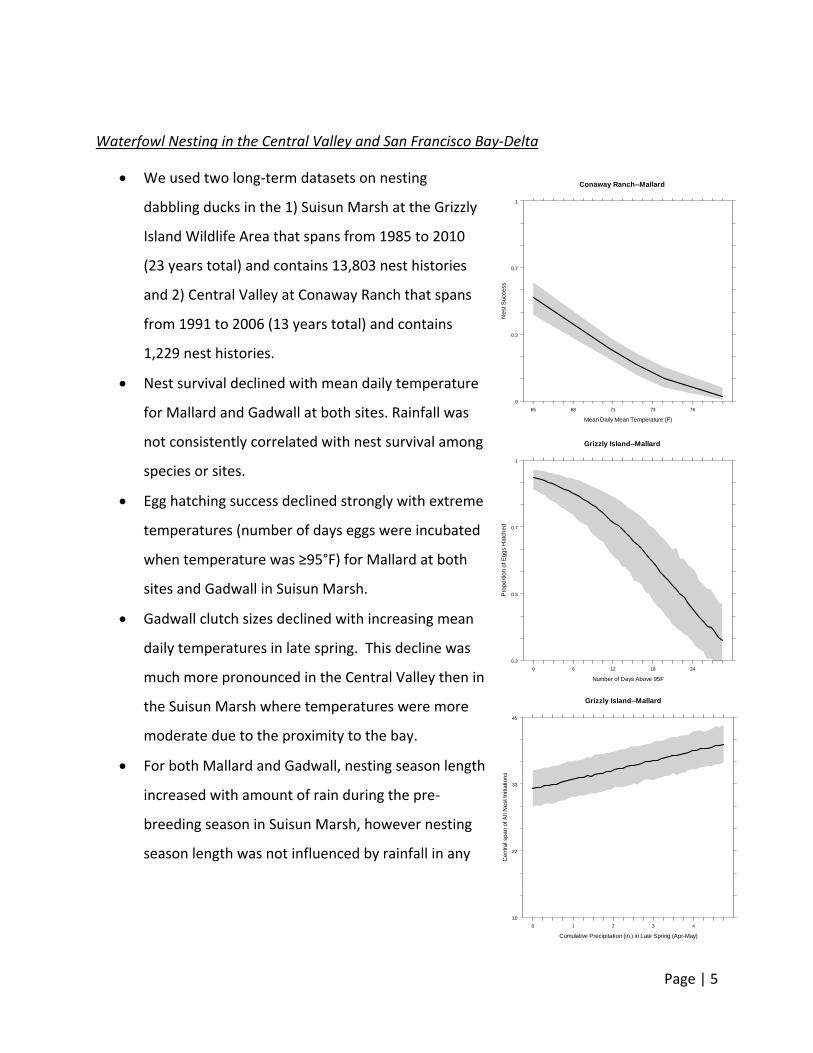
Waterfowl Nesting in the Central Valley and San Francisco Bay‐Delta

We used two long‐term datasets on nesting

dabbling ducks in the 1) Suisun Marsh at the Grizzly

Island Wildlife Area that spans from 1985 to 2010

(23 years total) and contains 13,803 nest histories

and 2) Central Valley at Conaway Ranch that spans

from 1991 to 2006 (13 years total) and contains

1,229 nest histories.

Nest survival declined with mean daily temperature

for Mallard and Gadwall at both sites. Rainfall was

not consistently correlated with nest survival among

species or sites.

Egg hatching success declined strongly with extreme

temperatures (number of days eggs were incubated

when temperature was ≥95°F) for Mallard at both

sites and Gadwall in Suisun Marsh.

Gadwall clutch sizes declined with increasing mean

daily temperatures in late spring. This decline was

much more pronounced in the Central Valley then in

the Suisun Marsh where temperatures were more

moderate due to the proximity to the bay.

For both Mallard and Gadwall, nesting season length

increased with amount of rain during the pre‐

breeding season in Suisun Marsh, however nesting

season length was not influenced by rainfall in any

Conaway Ranch--Mallard

Mean Daily Mean Temperature (F)

Ne

st S

ucc

ess

0

0.3

0.7

1

65 68 71 73 76

Grizzly Island--Mallard

Number of Days Above 95F

Pro

por

tion

of E

ggs

Hat

che

d

0.2

0.5

0.7

1

0 6 12 18 24


Cumulative Precipitation (in.) in Late Spring (Apr-May)

Ce

ntr

al s

pan

of A

ll N

est

Initi

atio

ns

10

22

33

45

0 1 2 3 4

se

In

th

w

M

G

M

C

Songbird

W

so

th

to

h

N

2

h

W

m

su

m

m

th

re

N

eason in the

n Suisun Mar

here was mo

with late spri

Mallard initia

Gadwall nest

Marsh, but ne

entral Valley

d Nesting at P

We used seve

ongbirds in t

he Palomarin

o 2008 (13 y

istories and

North San Fra

006 (11 yea

istories.

Wrentit nest

minimum tem

urvival in So

month minim

marshes whe

han at Palom

elated to any

Nest survival

e Central Val

rsh, Mallard

ore rain in la

ng rain.

ated nests ea

ing season le

esting seaso

y due to ear

Point Reyes

eral long‐ter

the 1) Point

n Research S

years total) a

2) tidal mar

ancisco Bay t

rs total) and

survival incr

mperature at

ng Sparrows

mum temper

ere temperat

marin. Songb

y other tem

was (slightly

ley.

, and to a le

te winter, a

arlier when s

ength decre

on length inc

lier nesting.

National Sea

rm datasets

Reyes Natio

Station that

and contains

rshes within

that spans f

d contains 3,0

reased with

t Palomarin,

s decreased

ature, espec

tures varied

bird nest sur

perature me

y) positively

sser extent G

nd nesting s

spring temp

ased with ea

creased with

a Shore and

on nesting

onal Sea Sho

spans from

s 1,049 nest

sites along t

rom 1996 to

020 nest

hatch‐mont

, but nest

with hatch‐

cially in tidal

more widel

vival was no

etric assesse

related to

Gadwall, init

season lengt

eratures we

arly spring te

h early spring

d North San F

re at

1996

the

o

th

l

y

ot

ed.

tiated nests

th (central sp

ere warmer i

emperature

g temperatu

Francisco Ba

Pag

later when

pan) increas

n Suisun Ma

es in Suisun

ures in the

ay

ge | 6

ed

arsh.

h

re

Songbird

D

ch

W

h

th

n

D

to

th

a

m

In

d

P

in

w

Climate C

B

in

ex

Eg

atch‐month

elated to hat

d Arrival Date

Date of first a

hanged over

Warbling Vire

as decrease

he observed

umbers.

Day of first ar

o large‐scale

hree Neotro

rrival date d

monthly valu

ndex, indicat

ate declined

acific‐slope

ncreased wit

warmer years

Change Proje

y 2070, clim

ncrease from

xpected to d

gg hatching

precipitatio

tch‐month p

es at Point R

arrival has no

r time for so

eo. Howeve

d in abunda

trend may b

rrival for son

e climate ind

pical migran

declined with

e of the Nor

ting later arr

d with ENSO

Flycatcher a

th the South

s.

ections – Wa

mate models

m 3.1o – 4.3oF

decrease by

success is p

on for Wrent

precipitation

Reyes Nation

ot significan

ongbirds, exc

r, Warbling

nce at Palom

be due to de

ngbirds was

dex variables

nts. Barn Sw

h the cumula

rthern Oscill

rival dates d

values, indi

arrival dates

ern Oscillati

aterfowl

project over

F, with incre

1.9 – 6.9 inc

rojected to d

tit at Paloma

n for tidal ma

nal Sea Shore

tly

cept for

Vireo

marin, so

eclining

related

s for only

wallow

ative

ation

uring El Niño

cating earlie

declined wit

ion Index, su

rall mean te

eased freque

ches.

decline for b

arin, but nes

arsh Song Sp

e

o years. Blac

er arrival dat

th the Pacifi

uggesting lat

mperatures

ency of heat

both Mallard

st survival wa

parrows.

ck‐headed G

tes during El

ic Decadal O

ter arrival da

in the Cent

waves, and

d and Gadwa

Pag

as negativel

Grosbeak arr

l Niño event

Oscillation an

ates during

ral Valley to

precipitatio

all at both si

ge | 7

y

rival

s.

nd

on is

tes.

T

th

a

C

G

N

C

m

se

n

Climate C

F

su

Pro

po

rtio

n o

f Eg

gs

Ha

tch

ed

0

0

his expected

he Central V

nd stabilizin

lutch sizes a

Gadwall in Su

Nesting seaso

entral Valley

mainly to the

eason, who

esting.

Change Proje

uture projec

urvival.

C

0

.3

.7

1

Present

d decline in h

Valley where

g properties

are projected

uisun Marsh,

on length is

y. Mallard n

e season end

initiate nest

ections – Son

ctions for the

onaway Ranch--Malla

2070 (3.1F Increase)

hatching suc

temperatur

s of the bay

d to decreas

, but less so

projected to

nesting seaso

ding earlier t

ts later in the

ngbirds

e Song Sparr

ard

2070 (4.8F Incre

ccess is espe

res can beco

and coastal

e by approx

for ducks ne

o change mo

on length is

han it curren

e season, is e

row and Wre

Pro

po

rtio

n o

f Eg

gs

Ha

tch

ed

0

0.3

0.7

1

Presentease)

ecially prono

ome extreme

regions.

ximately 6%

esting in the

ost dramatica

expected to

ntly does, w

expected to

entit sugges

Conaway R

(3.

ounced for d

ely high with

for Mallard

e Central Val

ally for duck

o shorten con

whereas the G

increase, du

st slightly en

Ranch--Gadwall

2070 .1F Increase)

Pag

ucks nesting

hout the coo

and 10% for

ley.

ks nesting in

nsiderably, d

Gadwall nes

ue to earlier

hanced nest


ge | 8

g in

oling

r

the

due

sting

r

t

Page | 9

Management Implications

Our results suggest that, in California, waterfowl demographics appear to be strongly

related to climate variables whereas songbird demographics are not. This could be due

in part to differences in habitat type among species, as many of the strongest

relationships with temperature occurred for ducks nesting in the Central Valley where

temperatures can be extremely hot without the moderating influence of the bay and

coastal regions.

Projections suggest that increased temperatures will have the strongest negative effects

on waterfowl egg hatching success. Management for dense nesting cover and

vegetation that provides shading for eggs later in the nesting season could improve

hatching success.

Future precipitation estimates are uncertain, but water will undoubtedly become an

increasingly scarce commodity for wildlife as use by agriculture and urban development

likely will increase in the future. Management actions to ensure waterfowl have access

to wetlands that are adjacent to nesting habitat will be essential.

Arrival dates for songbirds may differ in the future, with some species like Barn

Swallows arriving later and other species like Black‐headed Grosbeaks arriving earlier.

This potentially sets the stage for mismatches between resources and nesting

phenology.

Page | 10

Avian Demographic Response to Climate Change: A Multi‐Species and Multi‐Landscape Approach to Synthesizing Risk Factors Josh T. Ackerman and Mark P. Herzog

U.S. Geological Survey, Western Ecological Research Center, Davis Field Station, University of California‐Davis, Davis, CA

Leo Salas, Thomas Gardali, and Grant Ballard

PRBO Conservation Science, Petaluma, CA

Dan Loughman and Greg Yarris

California Waterfowl Association, Sacramento, CA

John M. Eadie

University of California‐Davis, Davis, CA

Introduction

The presence and persistence of a species on the landscape is determined by the complex

effects of biophysical variables on demographic parameters of populations of the species, such

as survival and productivity. Understanding the biophysical effects on avian demographics

provides a sound foundation for natural resource management, including more robust

predictions of future species distributions and species population viability. Management

actions can then be directly linked to demographic changes (Van Turnhout et al. 2010), such as

changes in nest survival.

Studies assessing how animal demographics have responded to climate variables can provide

insight on the drivers of population changes and for more robust predictions of future species

Page | 11

distributions and population viability (Both et al. 2006, Robinson et al. 2007, Wright et al. 2009).

In particular, knowing the conditions that are most favorable for bird nesting and nest survival

allows managers to more accurately identify, outline, restore, and manage landscapes and

regions for increased productivity (Seavy et al. 2008). Metrics of productivity and survival also

are necessary to properly estimate population trends. These are the building blocks of

population viability analyses. Determining the drivers of population changes allows for proper

modeling of future population scenarios.

Herein, we evaluate how avian demographic parameters are likely to respond to climate change

for a suite of species and provide a web‐based tool to assist natural resource managers with

understanding the potential future impacts of climate change and the specific effects of

environmental variables. We used two main guilds of birds, waterfowl and songbirds, and a

gradient of habitats from the Coast Range, through the San Francisco Bay, and into the Central

Valley of California.

Objectives

Specifically, we:

1) Assessed and synthesized several breeding demographic responses to climate change

variables (i.e., precipitation and temperature).

2) Created a web‐based application (within the California Avian Data Center [CADC];

http://data.prbo.org/apps/aviandemog/) that provides access to our findings and

supports the visualization and summarization of avian demographic data.

Background

We used the two largest datasets on breeding waterfowl in California (1985 – 2010) to compare

how the breeding demographic parameters of Mallard (Anas platyrhynchos) and Gadwall (Anas

strepera) differ with temperature and precipitation patterns between the two major breeding

habitats within the Central Valley and Suisun Marsh. We used long‐term (1996‐2008) nest

monitoring datasets collected and maintained by PRBO Conservation Science for bird species

breeding at the Palomarin Field Station in the Point Reyes National Sea Shore (hereafter

Palomarin), and locations in the tidal marsh along the north San Francisco Bay. Lastly, we used

Page | 12

one of the largest datasets in the country of constant‐effort banding data, from Palomarin, to

determine the date of first arrival of Neotropical and Nearctic migrant bird species, and its

relationship with four large‐scale climate indices.

Study Sites

Waterfowl data were collected at two locations: Conaway Ranch (38.6472 N, ‐121.6683 E) and

Grizzly Island Wildlife Area (38.1552 N, ‐121.9757 E). Conaway Ranch is located in the Central

Valley of California, just east of the towns of Woodland and Davis. Grizzly Island Wildlife Area is

located within the Suisun Marsh in the transition zone between the San Francisco Bay and the

Sacramento‐San Joaquin River Delta. Temperatures within the Central Valley can become

extremely hot during the summer, whereas Suisun Marsh temperatures are more moderate as

they are buffered by the large expanses of water within the San Francisco Bay and proximity to

the coast.

Songbird data were collected at two general study sites – the Palomarin Field Station, located

within the Point Reyes National Sea Shore, 20 Km north of the city of San Francisco, California,

and the San Francisco Bay northern tidal marshes (hereafter the “tidal marshes”) for Song

Sparrows [Melospiza melodia] only. The weather and vegetation at Palomarin has been

extensively documented elsewhere (e.g., Silkey et al. 1999, Chase et al. 2005). The site is

primarily a mixture of dense mature coastal scrub with encroaching Douglas fir (Pseudotsuga

menziesii), and an oak‐bay riparian area. The tidal marsh study site encompasses five specific

locations: China Camp (southwestern San Pablo Bay; ‐122.4956 E, 38.0123 N), Black John

Slew/Carl’s Marsh/Petaluma River Restoration Marsh/Petaluma River Mouth (‐122.5057 E,

38.1241 N), Pond 2A Restoration Marsh (on the Napa river east of San Pablo Bay; ‐122.32133 E,

38.153 N), Southampton/Benicia Marsh (‐122.1934 E, 38.0736 N), and Rush Ranch (north

Suisun Bay; ‐122.0268 E, 38.2022 N). All marshes are restoration sites at ≥10 years of age.

Dominant plant species include pacific cordgrass (Spartina foliosa) annual and perennial

pickleweed (Sarcocornia spp.), bulrushes (Bolboschoenus spp. and Schoenoplectus spp.), cattails

(Typha spp.), and shrubs, such as coyote bush (Baccharis pilularis).

Page | 13

Species Descriptions

Mallard (Anas platyrhynchos) and Gadwall (Anas strepera) are both waterfowl within the

Anatinae sub‐family, also called “dabbling ducks”. These species differ in their life history

strategies, with Gadwall having a “faster” life history strategy than Mallard, characterized by

having a higher reproductive output and shorter lifespans than Mallard (Ackerman et al. 2006).

Population estimates for Mallard in California is higher than for Gadwall, and while both species

are found year round within the Central Valley and Suisun Marsh, the number of Mallard

breeding in these areas are about 3 times higher than the number of breeding Gadwall. Mallard

are larger birds, but their reproductive output (i.e., clutch mass / body mass) is smaller than

Gadwall (Ackerman et al. 2006). Mallard lay an average of 9 eggs and incubate their clutch for

approximately 26 days, whereas Gadwall lay 11 eggs and incubate their clutch for

approximately 24 days (Klett et al. 1986). Both species nest on the ground in upland vegetation

near wetlands, and, at hatch, females lead precocial ducklings to water.

Song Sparrows are territorial passerines found in many kinds of open habitats throughout

North America and northern Mexico (Arcese et al. 2002), but particularly in riparian habitats

and marshes. The Marin subspecies, M. m. gouldii, found at Palomarin, the Suisun subspecies,

M. m. maxillaris, found in the tidal marshes around Suisun Bay, and the Samuel’s subspecies,

M. m. samuelis, found in San Pablo Bay, are all local breeders and year‐round residents

(Humple and Geupel 2004). Although primarily monogamous, males may mate with multiple

females. Clutch size is 2‐5 eggs, with incubation period lasting approximately 13 days and

nestling period about 9 days (Jongsomjit et al. 2007). At Palomarin a 3‐egg nest fledges chicks

in 24 days, whereas at the tidal marshes chicks fledges in 23 days. Wrentits (Chamaea fasciata)

are also year‐round territorial passerines, though more strictly monogamous than Song

Sparrows (Geupel and Ballard 2002). The species is confined to the coastal scrub and chaparral

habitats of Pacific North America. The most notable characteristic of the Wrentit, in contrast to

the Song Sparrow, is that the male helps in incubation, and both incubation and fledging

periods are longer. A 3‐egg clutch (clutches vary from 1 to 5 eggs) takes approximately 32 days

to fledge chicks at Palomarin (Geupel and Ballard 2002, Jongsomjit et al. 2007).

The species selected for the analysis of Date of First Arrival were chosen for their documented

sensitivity to climate and weather (MacMynowski et al. 2007; PRBO unpublished data) and high

capture rates. These include the following Neotropical migrants: Barn Swallow (Hirundo

Page | 14

rustica), Black‐headed Grosbeak (Pheucticus melanocephalus), Cliff Swallow (Petrochelidon

pyrrhonota), MacGillivray’s Warbler (Oporornis tolmiei), Northern Rough‐winged Swallow

(Stelgidopteryx serripennis), Olive‐sided Flycatcher (Contopus cooperi), Orange‐crowned

Warbler (Vermivora celata), Pacific‐slope Flycatcher (Empidonax dificilis), Swainson’s Thrush

(Catharus ustulatus), Warbling vireo (Vireo gilvus), Wilson’s Warbler (Dendroica pusilla), and

Yellow Warbler (Dendroica petechia). Three species of Nearctic migrants were selected for the

analysis as well: Fox Sparrow (Passerella iliaca), Golden‐crowned Sparrow (Zonotrichia

atricapilla) and Ruby‐crowned Kinglet (Regulus calendula).

Nest Monitoring Data and Methods

The Grizzly Island Wildlife Area dataset represents 23 years of breeding waterfowl data, and nearly 14,000 nests. Data have been collected at this site for every year since 1985, except for 2005‐2007 when funding was not available (Table 1). Conaway Ranch was monitored in 1991, and 1995‐2006 (Table 1), representing 13 years and over 1,000 nests. For detailed descriptions of the field methods used to collect waterfowl data see McLandress et al. (1996), Ackerman (2002), and Ackerman et al. (2003a,b,c, 2004). Nest searches were initiated each year in early April and continued until July to ensure finding both early‐ and late‐nesting ducks. The date of nest initiation was calculated by subtracting the age of the nest when found (i.e., the number of eggs when found plus the incubation stage when found) from the date the nest was discovered. Each field was searched four to five times at 3‐week intervals until no new nests were found. Nest searches began at least 2 hours after sunrise and were finished by 1400 hours to avoid missing nests due to morning and afternoon incubation recesses by females. Nest searches were conducted using a 50‐m nylon rope strung between two slow‐moving all‐terrain vehicles. Tin cans containing stones to generate noise will be attached at 1.5‐m intervals along the length of the rope. The rope was dragged through the vegetation, causing females to flush from their nests, thus enabling observers to locate nests by searching a restricted area. Nests were marked with a 2‐m bamboo stake placed 4 m north of the nest bowl and a shorter stake placed just south of the nest bowl, level with the vegetation height. Each nest was revisited on foot once every seven days, the stage of embryo development was determined by candling, and clutch size and nest fate were recorded. After each visit, we covered the eggs with nest materials (i.e., down and contour feathers from the nest), as the female would have done before leaving for an incubation recess.

Page | 15

Table 1. Total number of nests monitored at Grizzly Island Wildlife Area, Conaway Ranch, Palomarin

Research Station, and North Bay tidal marsh locations.

Nest searching and monitoring at Palomarin began in 1980 and is ongoing; the dataset used

here includes years 1996 to 2008. All nests were located at various stages (from building to

nestling periods) and were monitored using a standard protocol designed to minimize human

disturbance (Martin and Geupel 1993). The number of days between visits varied (1‐14 days,

mode = 3 days), though effort was made to visit every 2‐4 days to increase accuracy in

estimates of date of predation or abandonment, and egg laying. We reviewed the records and

discarded any data pertaining to building stages, or records of nests whose clutch date was

unknown or could not be estimated, resulting in a dataset with 437 nests of Song Sparrow and

612 nests of Wrentit monitored between 1996 and 2008; totaling 3,778 records of nest checks

(Table 1). Nest search and monitoring at the tidal marsh sites followed the same

abovementioned methodology. Search and monitoring of nests at the tidal marsh locations

began in 1996 and continued through 2007. Not all five locations contain nest records for all

years, since not all were surveyed throughout the period. The tidal marsh dataset includes

records for 3,020 Song Sparrow nests, totaling 12,315 nest check records (Table 1).

The banding methods used at Palomarin follow the general methodology outlined in Ralph et

al. (1993). Full details can be found in the California Avian Data Center

(http://data.prbo.org/cadc2/index.php?page=songbird‐tools) and in Gardali et al. (2000). The

banding station has been running year‐round since 1965, with standardized sampling effort

since 1979. For this reason, we include only data for captures between 1979 and 2009. A total

of 20 nests are monitored 6‐7 days each week for 6 hours. We used only data for each species

Study Site 1985 1986 1987 1988 1989 1990 1991 1992 1993 1994 1995 1996 1997

Grizzly Island 508 590 632 667 564 376 621 765 491 1107 1005 1181 819

Conaway Ranch - - - - - - 64 - - - 146 183 85

Palomarin - - - - - - - - - - - 123 89

Tidal Marshes - - - - - - - - - - - 154 346

Study Site 1998 1999 2000 2001 2002 2003 2004 2005 2006 2007 2008 2009 2010 Total

Grizzly Island 656 483 537 425 284 384 169 - - - 333 304 902 13803

Conaway Ranch 123 70 60 48 55 51 83 179 82 - - - - 1229

Palomarin 130 47 72 62 104 125 79 93 46 66 13 - - 1049

Tidal Marshes 172 346 181 310 344 128 247 441 351 - - - - 3020

Page | 16

and year spanning the date of first capture and the subsequent 20 banding days, including

records from new captures of adult individuals only (i.e., after‐hatch year or older).

Avian Breeding Demographic Parameters

Climate has the potential to not only influence when birds initiate nests, but how long they can

keep nesting, or how many nests can be initiated. Climate variables also can extend beyond

phenology, by directly influencing the nest survival, or the hatching success of individual eggs.

Thus, to fully assess the impacts that climate, seasonal, and daily weather conditions can have

on breeding waterfowl in California, we modeled a large suite of breeding parameters that

represent all periods and facets of the nesting season (Table 2). For songbirds, we focused only

on nest survival.

For the waterfowl data analyses, breeding parameters were estimated at either the individual

level or the site level, depending on what was most appropriate. Nest survival, clutch size,

hatching success (i.e., proportion of eggs that hatched in a successful nest), and the initiation

date of a nest were all summarized at the individual nest level. Breeding season length was

estimated at the site level.

Below, we provide methods for estimating each breeding parameter, as well as some of our

thinking as we developed suites of a priori hypotheses related to how weather and climate

might affect each of these demographic parameters.

Clutch Size

Method of estimation ‐ Clutch size was defined as the total number of eggs laid in the nest. Only

nests that were found within 8 days of laying and showed no signs of partial depredation

(Ackerman et al. 2003a) were included in our analyses.

Candidate set of covariates – It is assumed that ducks obtain most of the resources required for

egg formation on the breeding grounds. Thus, any weather variables that may influence what

resources will be available in the breeding area in the 2‐3 weeks prior to a nest being initiated

were included. Since nests were initiated until late June/early July, we selected variables that

could influence invertebrate production, and included mean and minimum temperatures in all

Page | 17

monthly groupings (see Table 3) as well as cumulative precipitation. It is also well documented

in the literature that clutch size in ducks declines throughout the breeding season. Thus we

added the date of nest initiation as an additional covariate. We did not include any 2‐way

interactions and restricted any single model to a maximum of 8 parameters.

Table 2. Breeding demographic parameters estimated from the data.

Response variable Species Definition

Clutch size Waterfowl Clutch size by nest

Nest initiation date Waterfowl Nest initiation date by nest

Proportion of eggs hatched

Waterfowl Proportion of eggs within a clutch that hatched from a successful nest

Central span of nesting season

Waterfowl

Central span of nesting season length (number of days between when 10% and 90% of all nests were initiated)

10th percentile nest initiation date

Waterfowl Date when 10% of all nests were initiated

90th percentile nest initiation date

Waterfowl Date when 90% of all nests were initiated

Daily nest survival probability

Songbirds & waterfowl

Probability of daily nest survival of a nest

Probability of nest survival

Songbirds Probability of nest surviving from clutch completion to fledging date

Date of first arrival Songbirds Date the species was first detected at Palomarin

Page | 18

Table 3. Delineations of seasons used to summarize weather covariates.

Season Months

late.winter December ‐ January

early.spring February ‐ March

late.spring April ‐ May

early.summer June ‐ July

Nest Initiation Date, Central Span of Nesting Season, and 10th and 90th Percentile of Nests

Initiated

Method of estimation – Nest initiation date was defined as the date at which an individual

female laid the first egg in the nest. Only nests where researchers were confident that nest

initiation date could be estimated were included. Nest initiation date was estimated by

subtracting the initial clutch size plus the average incubation stage of all eggs in the clutch on

the day the nest was first discovered from the date the nest was found. In addition to the

estimation of each nest’s individual initiation date, estimates of the dates when 10% and 90%

of nests were initiated for each site (nesting field) within each region. In addition, the central

span of nests, or number of days between the dates when 10% and 90% of all nests within a

site were initiated, was estimated as a metric for the duration of the nesting season.

Candidate set of covariates – We selected variables we believed would influence the availability

and timing of suitable nesting habitat for ducks. In general, ducks prefer to nest in dense cover

within larger fields that are within a reasonable distance to water to support ducklings after

hatch. Thus, variables that would affect the condition of habitats within nesting fields (e.g.,

precipitation and temperature in winter and spring) were selected (Appendix 2). The end of

nest initiations during a season is a combination of available resources and life history

constraints. Warmer conditions and changed habitats later in summer may reduce the

availability of the specific resources necessary for egg formation. Thus, we hypothesized that

the termination of nesting would be influenced by conditions in late spring and early summer

primarily, though we deemed it possible that early spring weather may build the foundation for

how long resources were available.

Page | 19

Proportion of Eggs Hatched (Hatching Success)

Method of estimation – Hatching success is defined as the proportion of eggs that hatched

within a nest that was successful (i.e., where at least 1 egg hatched). Thus, only successful

nests where full clutch size and final fate for each individual egg was known were included in

our analyses (after Ackerman et al. 2003a).

Candidate set of covariates – We hypothesized that extremely hot temperatures for longer

periods of time may exceed an incubating female’s ability to protect the eggs from over‐

heating. Whereas it is possible that thermal stress may also influence overall nest survival (see

below), thermal stress may also only influence a fraction of eggs depending on their location in

the nest bowl. Variables we selected a priori represented either immediate or direct effects of

temperature for that nest (e.g., number of days during the incubation period where

temperatures exceeded 95°F), as well as overall general seasonal temperature measures

(Appendices 2 & 4).

Nest Success ‐ Waterfowl

Method of estimation – Nest success for each site was estimated as the product of modeled

daily survival rate estimates for each day of an average nest. A nest starts on the day the first

egg is laid in the nest, and continues through the period of egg laying (9 days for Mallard and 11

days for Gadwall) and incubation (26 days for Mallard and 24 days for Gadwall). Thus, each

Mallard and Gadwall nest must successfully survive 35 days to be successful. Nest survival was

estimated separately for each region and species using the nestsurvival (Herzog 2011) package in R, and was based on the logistic exposure model (Shaffer 2004). A successful nest

was defined as a nest where at least 1 egg hatched. For some nests, it was possible to

determine the exact date of the nest’s fate. However, in most cases, the final nest fate date

was estimated in the same manner as is done for Mayfield nest success; that is, the date that

represents the midpoint of the final visit interval when the nest fate was determined (Mayfield

1961, Mayfield 1975, Johnson 1979). Only nests where at least 1 day of exposure occurred

were included in analyses.

Candidate set of covariates – Model selection was performed in a two‐step process. First, we

developed a base model, by assessing all possible models associated with date, nest age, age of

Page | 20

nest when found, relative nest initiation date (relative to other nests in the given year and

region), and year, including squared terms for most variables (see Appendices 2 & 4). For all

regions and species, the data strongly supported 2 models. Both models were identical (single

linear combinations of all variables), differing only by the inclusion (or exclusion) of “age when

found”. Since the favored model among the analyses was not consistent and never > 2 AICc

different, and because of our belief that survival might be inherently different for nests found

when they are older, we included the variable “age when found” in our base model.

Nest Success ‐ Songbirds

Method of estimation ‐ We constructed 73 different competing generalized linear models with

a logistic‐exposure model (i.e., a logistic link constructed as described by Shaffer 2004) using

the R package nestsurvival (Herzog 2011) using a very similar approach to that described

within the waterfowl section. We evaluated combinations of the climatic variables that would

account for the three biophysical parameters described below. Additionally, we accounted for

the possibility that the daily survival rate could vary throughout the life of the nest by including

a linear, quadratic, or cubic parameter for the age of the nest. Similarly, the daily survival rate

also may vary depending on the date of the nest with respect of the beginning of the nesting

season, so that nest attempts at the beginning and end of the season may be less successful

than those in the middle. We accounted for this effect by adding linear, quadratic, or cubic

parameters for the date of the nest with respect to the beginning of the season (the first clutch

date for each year). Lastly, we considered the possibility of unaccounted for variance between

years by modeling year as a discrete explanatory variable.

The response parameter of the models, survival of the nest to the exposure interval (the

interval between nest checks), was scored by determining whether the nest was still active or

had successfully fledged at least one young, or was depredated/abandoned at the end of the

interval. We thus assigned 1’s or 0’s respectively to each check. We omitted first observation

records unless these coincided with the clutch date (i.e., left censoring of records to avoid

artificially inflating the survival estimates by considering only nests known to have survived

until they were discovered). We assigned an age of the nest as the middle day of the interval

between checks, and a date of the nest in the season as the date of the middle of the interval

with respect to the first clutch date for the appropriate year.

Page | 21

Variable importance was evaluated directly from each model fit in the set of competing models

by simply counting the number of models in which the variable contributed significantly (p‐

value <0.05) to the fit.

Predicting to the future climate scenarios was done by attributing all current records with the

future temperature and precipitation values under either one of the two models we

considered. We then averaged the value of each climatic variable in the data and used these

average values to predict with the set of competing models. Thus the resulting predicted future

survival probabilities reflect variance across locations and model uncertainty.

Candidate set of covariates for songbirds ‐ We first calculated 13 derivative environmental

variables from the PRISM variables and the future climate datasets, listed in Appendix 2. Each

one of these is intended to be a proxy measurement of three potentially important biophysical

parameters potentially affecting the survival probability of Song Sparrows and Wrentits. The

first parameter known to affect Song Sparrow nest survival is precipitation in the prior rainy

season (Chase et al. 2005). How much vegetation growth and insect productivity may occur at

the sites is likely largely dependent on the amount of precipitation in the rainy season (between

October and March, hereafter bioyear precipitation). Chase (2002) speculate that the amount

of bioyear precipitation is directly associated with the amount of foliage that provides for nest

cover. On low precipitation years nest cover is poor and predation is high, and vice versa. We

also considered precipitation one to three months prior to the hatch month as proxy measures

of vegetation growth and productivity. Competing models had one of these variables. The

second parameter potentially affecting nest survival is minimum and maximum temperature

one to three months prior to the hatch month (Chase et al. 2005). Lastly, DeSante and Geupel

(1987) observed a large proportion of nests abandoned during a nesting period of particularly

high rainfall. Chase et al. (2005) also investigated the effect of temperatures to nest survival.

Thus, we evaluated the effect of total precipitation and minimum and maximum temperature

during the hatch month.

Date of First Arrival

Method of estimation ‐ For each year and each species, day of first arrival was estimated as the

intercept parameter of the regression of date against the cumulative capture rate in the

banding data; that is, the point when the cumulative capture rate is 0 just before the first

Page | 22

capture is made. The date was converted to days since vernal equinox to reduce bias that

changes in timing of actual spring can have on calendar dates (Sagarin 2001).

Candidate set of covariates ‐ Since climatic conditions affecting arrival dates may not be those

of the winter or summer grounds (for Neotropical or Nearctic migrants, respectively), we

explored parameters derived from four large scale climate indices to correlate to the arrival

date estimates. Species abundance patterns and fecundity also correlate with patterns of date

of first arrival (Miller‐Rushing et al. 2008) and are affected by many other parameters not

considered here (Gordo 2007).

Climatic Covariates and Analysis Methods

Weather Data – Waterfowl Analyses

Weather covariates (see Appendix 1) used in waterfowl data analyses were summarized from

daily weather station data collected at weather stations near each study area and downloaded

from the National Climate Data Center (NCDC; http://www.ncdc.noaa.gov). Units are

presented as received from NCDC as degrees Fahrenheit (°F) for temperature, and inches for

cumulative precipitation.

Given the unique location of Grizzly Island Wildlife Area, and lack of weather data in the

immediate vicinity, we were concerned that weather data would not adequately represent the

region. Weather data, however, had been collected at Grizzly Island Wildlife Area in early years

(1971‐1977). Therefore, we retrieved daily weather data from several stations within the area

(cities of Antioch, Fairfield, Martinez, and Vacaville) as well as Grizzly Island Wildlife Area for the

period 1970‐1979. Using the hclust procedure (Venables and Ripley 2002) in R, we performed agglomerative hierarchical clustering (Gordon 1999) to understand which sites were

most similar to each other with respect to precipitation (total daily accumulation) and

temperature data (minimum, mean, and maximum daily temperature). These results suggested

that weather in Antioch and Fairfield were much more similar to Grizzly Island Wildlife Area

weather than either Martinez or Vacaville. We then performed simple regressions with Grizzly

Island Wildlife Area weather data as the response variable and Antioch and Fairfield weather as

covariates to understand how the information from each of these stations contributed to the

Grizzly Island Wildlife Area weather station data. Results indicated that temperature could be

represented approximately as the weighted average of 0.6*Fairfield temperature and

Page | 23

0.4*Antioch temperature (R2 = 0.98). For precipitation, Grizzly Island Wildlife Area rainfall was

approximated by the weighted average of 0.4*Fairfield precipitation and 0.6*Antioch

precipitation (R2 = 0.65). Given the difference between temperature and weather relationships

and since this comparison was made on a small amount of data many years prior to our actual

study, we opted to simply take the mean of the Antioch and Fairfield daily weather station data

to represent all Grizzly Island Wildlife Area weather during our study. Validating this

relationship, showed that it had little effect on the relationship (temperature R2 = 0.96;

precipitation R2 = 0.61).

Conaway Ranch weather data was much more straightforward. Situated equidistant from both

Davis and Woodland weather stations, we took the combined mean daily weather data from

the cities of Davis and Woodland to represent the weather at Conaway Ranch.

For both Grizzly Island Wildlife Area and Conaway Ranch, when daily weather data were not

available for 1 weather station, only weather data from the second weather station was used.

Weather Data – Songbird Analyses

Climate data for the Song Sparrow and Wrentit data analyses were downloaded from the

PRISM project (PRISM 2011), thus including monthly minimum and maximum temperatures and

monthly total precipitation. The PRISM datasets are grids of 4 x 4 km, so the entire Palomarin

dataset was included within a single cell of the PRISM grid. All six locations from the tidal

marsh dataset are in different cells of the PRISM dataset. Since the climate data are

extrapolated from nearby weather stations based on geomorphological attributes, the tidal

marsh locations showed little difference in climate parameter values.

Future scenario data for the songbirds were obtained for a single average year (averaged for

the 30 years between 2040 and 2070) based on projections from a regional climate model,

RegCM3, with emission trajectory taken from the Intergovernmental Panel on Climate Change

A2 scenario and boundary conditions based on output from two global circulation models. A

full description of the future dataset is provided by Stralberg et al. (2009).

We used the following four large scale climate indices: El Niño Southern Oscillation Index (ENSO

– http://www.coaps.fsu.edu/jma.shtml), Pacific Decadal Oscillation Index (PDO –

http://jisao.washington.edu/pdo/PDO.latest), Southern Oscillation Index (SOI), and Northern

Oscillation Index (NOI) (both found at:

Page | 24

http://www.pfeg.noaa.gov/products/PFEL/modeled/indices/NOIx/noix_download.html). These

links provide full description of the indices. We evaluated three parameters derived from these

indices that we expected may influence date of first arrival for each species: sum of monthly

index values from October to December of the previous year, sum of index values from January

to March of the arrival year, and sum of index values from October to March.

All analyses were performed in the statistical programming language R (version 2.13.0; R Core

Development Team 2011).

Statistical Methods

Waterfowl

We used a consistent approach for modeling all breeding parameters. For waterfowl, analyses

were performed for each combination of species (Mallard and Gadwall) and region (Grizzly

Island Wildlife Area and Conaway Ranch) separately. Thus, a total of four analyses were

completed on each of the breeding variables. We used a linear mixed model approach (Pinheiro

and Bates 2000) with year and site (nesting fields within each region) as random effects. For

each breeding parameter, we developed a set of plausible candidate models from the available

suite of weather covariates (see Appendices 2 & 4).

The candidate model set consisted of all possible linear combinations of the weather covariates

selected. The result was a very large set of possible models and a complete candidate model set

consisting of between 31‐255 models, depending on the breeding parameter. All candidate

models were run and model inference diagnostics were calculated for each model (Burnham

and Anderson 2002). For predictions and figures, we model‐averaged the suite of best models

that contributed 99% of the total model weight (as calculated by the AICC weights for each

model within the given model set). Model averaged predictions were derived from 1000

simulations of each model within the model set (Gelman and Hill 2007). Predictions and 95%

credible intervals are presented as the mean, 5th percentile, and 95th percentile from these

simulations (Gelman et al. 2003).

Page | 25

Songbirds

To estimate nest survival probabilities for songbirds, we fit models to each species and location

separately, thus resulting in three analyses for daily and nesting survival. The models for the

songbirds considered the possibility of unaccounted variance between years by modeling year

as a discrete explanatory variable. We considered only the set of models within 2 AIC units of

the top model as the competing model set (Burnham and Anderson 2002). This resulted in 10‐

14 competing models to estimate the nest survival probabilities for each species and location.

As with waterfowl analyses, for each breeding parameter we developed a set of plausible

candidate models from the available suite of weather covariates (see Appendix 1). The nest

survival estimates by year were then obtained by averaging the predicted survival values from

each model, weighted by the goodness of each model fit (AIC weights).

For the analysis of day of first arrival patterns, we sought to detect the significant contribution

of any of the three parameters derived from the large‐scale climate indices. We did not pursue

construction of predictive models. We restrict our discussion to how these parameters affect

arrival to speculate how future higher frequency of particular index values (i.e., global climatic

conditions) may affect arrival.

Results

We creat

provides

data. Res

http://da

and Discu

ted a web‐ba

access to ou

sults can be

ata.prbo.org

ussion

ased applica

ur findings a

visualized by

g/apps/avia

ation within

and visualiza

y natural res

andemog

the Californ

tion tools w

source mana

ia Avian Dat

which summa

agers at our

ta Center [CA

arize our avi

project web

Page

ADC] that

an demogra

bsite:

e | 26

aphic

Page | 27

Waterfowl Results

Clutch size

For all species and sites, clutch size declined with nest initiation date (β = ‐0.05 to ‐0.03

eggs/day), and represented a reduction of 1‐2 eggs throughout the entire breeding season

(mean breeding season length was 43 days; Figure 1). At all sites, weather covariates

representing temperatures during early and late spring were in the top models based on AICc

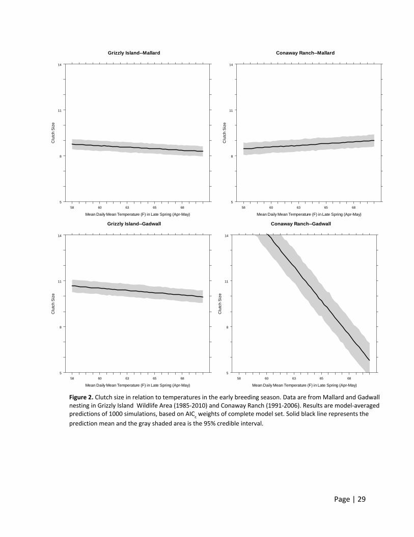
(Figure 2). Gadwall clutch size consistently declined with temperature in late spring (April –

May). Although present in the top models, Mallard clutch size did not show a consistent pattern

with temperature between study sites, nor did the slope estimates of the relationship deviate

significantly from zero.

The strong negative effect of temperature on Gadwall clutch size at Conaway Ranch is

complicated by small samples sizes (<150 nests for all years) and possibly confounded with the

remaining covariates that also were supported. However, we still believe these models support

a hypothesis that increasing temperatures may play a role in declining clutch sizes in the

summer for Gadwall, and could play an increasingly important role in the future when

conditions are expected to be warmer.

Page | 28

Figure 1. Clutch size declines during the breeding season in California waterfowl. Data are from Mallard and Gadwall nesting at Grizzly Island Wildlife Area (1985‐2010) and Conaway Ranch (1991‐2006). Results are model‐averaged predictions of 1000 simulations, based on AIC

c weights of complete model set. Solid black line

represents the prediction mean and the gray shaded area is the 95% credible interval. X‐axis represents all dates when a nest was found. In any given year, however, the typical breeding season is only 31‐53 (mean 42.8) days long.


Initiation Date (Days since January 1)

Clu

tch

Siz

e

5

8

11

14

57 89 122 154 186

Grizzly Island--Gadwall


Clu

tch

Siz

e

5

8

11

14

57 89 122 154 186



Clu

tch

Siz

e

5

8

11

14

57 89 122 154 186

Conaway Ranch--Gadwall


Clu

tch

Siz

e

5

8

11

14

57 89 122 154 186

Page | 29


Mean Daily Mean Temperature (F) in Late Spring (Apr-May)

Clu

tch

Siz

e

5

8

11

14

58 60 63 65 68



Clu

tch

Siz

e

5

8

11

14

58 60 63 65 68



Clu

tch

Siz

e

5

8

11

14

58 60 63 65 68

Figure 2. Clutch size in relation to temperatures in the early breeding season. Data are from Mallard and Gadwall nesting in Grizzly Island Wildlife Area (1985‐2010) and Conaway Ranch (1991‐2006). Results are model‐averaged predictions of 1000 simulations, based on AIC

c weights of complete model set. Solid black line represents the

prediction mean and the gray shaded area is the 95% credible interval.



Clu

tch

Siz

e

5

8

11

14

58 60 63 65 68

Page | 30

Initiation Date, Central Span of Nesting Season, and 10th and 90th Percentile of Nests Initiated

Relationships between breeding phenology variables and weather covariates were highly

variable, reflecting both the different systems that Grizzly Island and Conaway Ranch represent

as well as the difference in breeding ecology between Mallard and Gadwall.

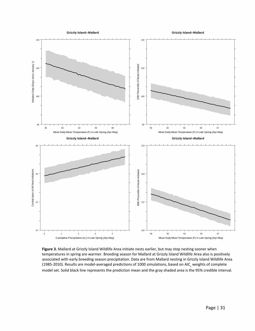
At Grizzly Island Wildlife Area, Mallard initiated nests earlier when spring temperatures were

warmer (Figure 3), and decreased nest initiation dates by nearly 2 days for every 1°F increase in

average daily temperatures in late spring. In addition, the nesting season length (central span)

for Mallard increased approximately 1.75 days for each additional 1 inch of cumulative rain that

occurred in late spring (Figure 3). In support of these relationships, the date when 10 percent of

all nests were initiated (representing the onset of the nesting season) was 1.41 day earlier for

each 1°F warmer Grizzly Island Wildlife Area was in late spring. The date when 90 percent of all

nests had been initiated (representing the end of nest initiation) also was 1.71 days earlier for

every 1°F warmer in spring.

Mallard, and to a lesser extent Gadwall, at Grizzly Island Wildlife Area initiated nests later when

there was more precipitation in late winter (1.93 and 0.84 days later for each additional 1 inch

of rain in the winter, respectively). For both species, at Grizzly Island Wildlife Area there was a

positive relationship between nesting season length and increased pre‐breeding precipitation

(see Appendix 2), however at Conaway Ranch nesting season was not influenced by the

amount of precipitation in any season.

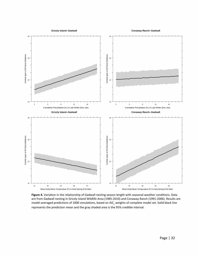
Whereas Gadwall at Grizzly Island Wildlife Area responded to increased late winter rains with

an increased nesting season duration (0.75 more days per 1 inch of winter rain), our data did

not support a similar relationship for Gadwall at Conaway Ranch (Figure 4). Likewise, Gadwall

responded differently to early spring temperature. Gadwall nesting season length decreased 1

day per 1°F increase in early spring temperatures at Grizzly Island Wildlife Area, but was 3 days

longer for each 1°F increase in early spring temperatures at Conaway Ranch (Figure 4).

A possible explanation for this contradiction among breeding sites on the influence that

temperature has on nesting season length is the negative correlation between cumulative

precipitation and mean temperatures in late spring (r= ‐0.56). Interestingly, this correlation

does not exist in early spring (r=‐0.02).

Page | 31

Figure 3. Mallard at Grizzly Island Wildlife Area initiate nests earlier, but may stop nesting sooner when temperatures in spring are warmer. Breeding season for Mallard at Grizzly Island Wildlife Area also is positively associated with early breeding season precipitation. Data are from Mallard nesting in Grizzly Island Wildlife Area (1985‐2010). Results are model‐averaged predictions of 1000 simulations, based on AIC

c weights of complete

model set. Solid black line represents the prediction mean and the gray shaded area is the 95% credible interval.



Initi

atio

n D

ate

(D

ays

sin

ce J

an

ua

ry 1

)

80

100

120

140

58 60 63 65 68



10

th P

erc

en

tile

of N

est

s In

itia

ted

80

100

120

140

58 60 63 65 67


Cumulative Precipitation (in.) in Late Spring (Apr-May)

Ce

ntr

al s

pa

n o

f All

Ne

st In

itia

tion

s

10

22

33

45

0 1 2 3 4



90

th P

erc

en

tile

of N

est

s In

iitia

ted

120

137

153

170

58 60 63 65 67

Page | 32


Mean Daily Mean Temperature (F) in Early Spring (Feb-Mar)

Ce

ntr

al s

pa

n o

f All

Ne

st In

itia

tion

s

10

22

33

45

51 53 54 56 57


Mean Daily Mean Temperature (F) in Early Spring (Feb-Mar)

Ce

ntr

al s

pa

n o

f All

Ne

st In

itia

tion

s

10

22

33

45

51 52 53 55 56


Cumulative Precipitation (in.) in Late Winter (Dec-Jan)

Ce

ntr

al s

pa

n o

f All

Ne

st In

itia

tion

s

10

22

33

45

2 5 9 12 16

Figure 4. Variation in the relationship of Gadwall nesting season length with seasonal weather conditions. Data are from Gadwall nesting in Grizzly Island Wildlife Area (1985‐2010) and Conaway Ranch (1991‐2006). Results are model‐averaged predictions of 1000 simulations, based on AIC


represents the prediction mean and the gray shaded area is the 95% credible interval.


Cumulative Precipitation (in.) in Late Winter (Dec-Jan)C

en

tra

l sp

an

of A

ll N

est

Initi

atio

ns

10

22

33

45

2 5 9 12 16

Page | 33

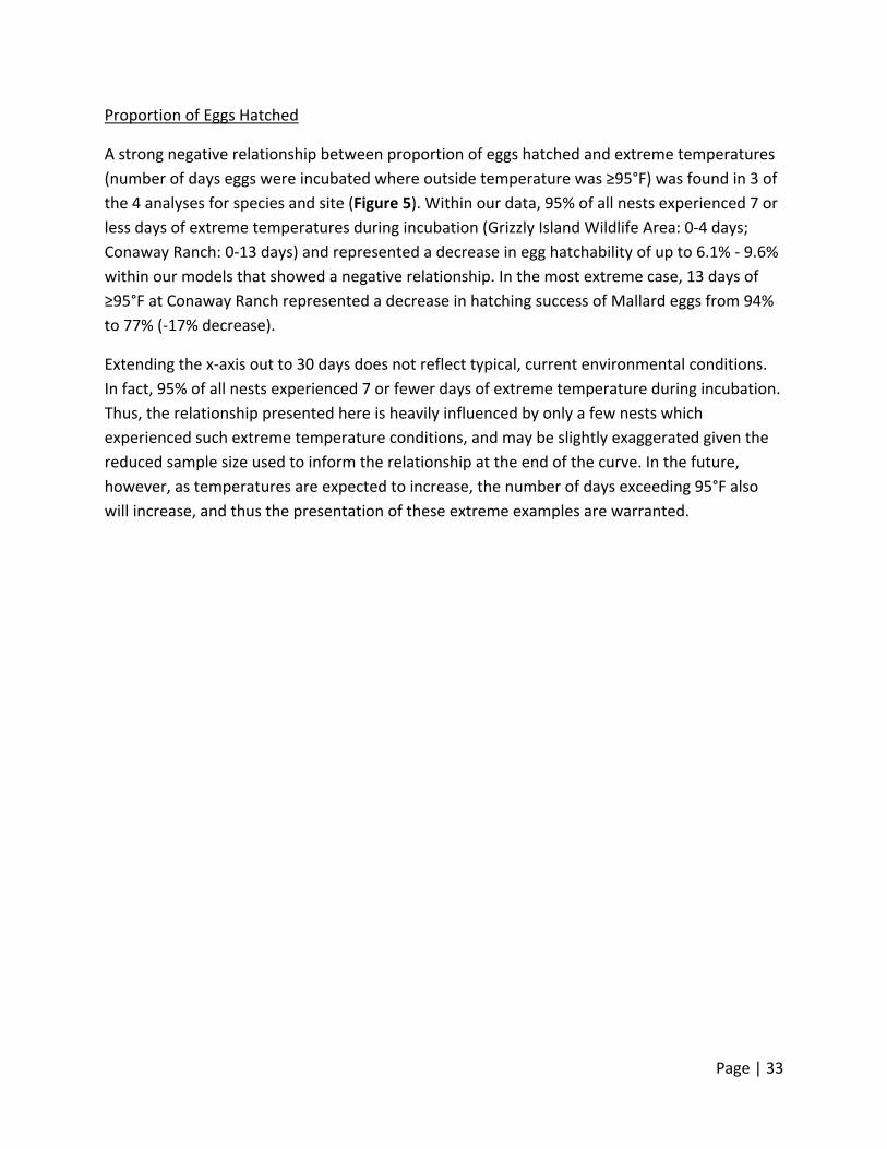
Proportion of Eggs Hatched

A strong negative relationship between proportion of eggs hatched and extreme temperatures

(number of days eggs were incubated where outside temperature was ≥95°F) was found in 3 of

the 4 analyses for species and site (Figure 5). Within our data, 95% of all nests experienced 7 or

less days of extreme temperatures during incubation (Grizzly Island Wildlife Area: 0‐4 days;

Conaway Ranch: 0‐13 days) and represented a decrease in egg hatchability of up to 6.1% ‐ 9.6%

within our models that showed a negative relationship. In the most extreme case, 13 days of

≥95°F at Conaway Ranch represented a decrease in hatching success of Mallard eggs from 94%

to 77% (‐17% decrease).

Extending the x‐axis out to 30 days does not reflect typical, current environmental conditions.

In fact, 95% of all nests experienced 7 or fewer days of extreme temperature during incubation.

Thus, the relationship presented here is heavily influenced by only a few nests which

experienced such extreme temperature conditions, and may be slightly exaggerated given the

reduced sample size used to inform the relationship at the end of the curve. In the future,

however, as temperatures are expected to increase, the number of days exceeding 95°F also

will increase, and thus the presentation of these extreme examples are warranted.

Page | 34



Pro

po

rtio

n o

f Eg

gs

Ha

tch

ed

0.2

0.5

0.7

1

0 6 12 18 24



Pro

po

rtio

n o

f Eg

gs

Ha

tch

ed

0.2

0.5

0.7

1

0 6 12 18 24



Pro

po

rtio

n o

f Eg

gs

Ha

tch

ed

0.2

0.5

0.7

1

0 6 12 18 24



Pro

po

rtio

n o

f Eg

gs

Ha

tch

ed

0.2

0.5

0.7

1

0 6 12 18 24

Figure 5. Proportion of eggs hatched from a successful nest decreases as the number of extreme temperatures days during incubation increases. Data are from Mallard and Gadwall nesting at Grizzly Island Wildlife Area (1985‐2010) and Conaway Ranch (1991‐2006). Results are model‐averaged predictions of 1000 simulations, based on AIC

c weights of complete model set. Solid black line represents the prediction mean and the gray shaded area is

the 95% credible interval.

Page | 35

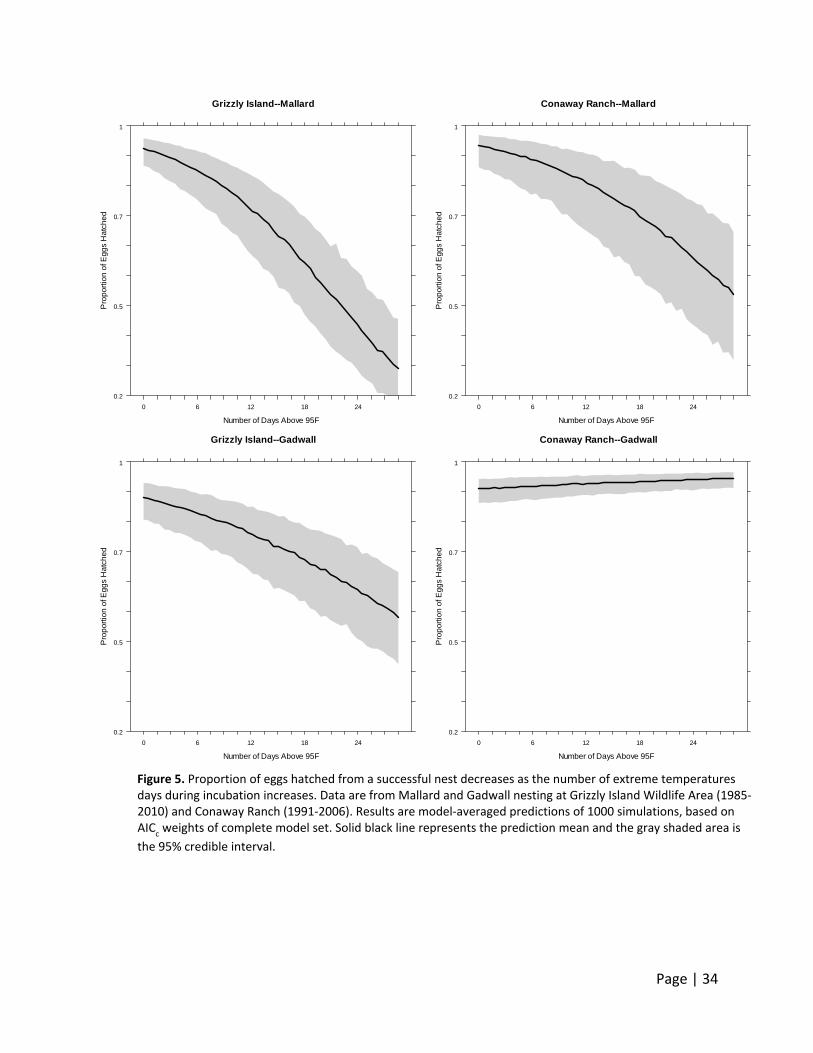
Nest Survival

Mallard and Gadwall nest success declined with relative nest initiation date at Grizzly Island

Wildlife Area (Figure 6). However, Mallard nest success increased and Gadwall nest success

decreased with relative nest initiation date at Conaway Ranch (Figure 6). The difference in

trends for the earlier nesting Mallard among sites are interesting, and suggests that in the

Central Valley nest survival increases as the season progresses and more water becomes

available as rice fields become flooded later in the season. A similar result of increasing

duckling survival with date in the Central Valley was found by G. Yarris (unpublished data), who

attributed higher survival of ducklings later in the nesting season to increased rice vegetation

cover to conceal ducklings from predators.

Daily nest survival declined with mean daily temperature for each species and site (Figure 7).

Precipitation metrics, both interval‐level as well as seasonal values, were not consistently

correlated with nest survival among species or sites and probably reflects the inherently

different habitats of Conaway Ranch and Grizzly Island Wildlife Area, as well as the ecological

differences between Mallard and Gadwall.

Of note, the base models (models developed prior to incorporation of weather covariates – see

Methods section) were very different among regions and species. This suggests there are

substantial ecological differences among these sites (such as differences in predator

community, land management, etc.) and is an area of active research.

Page | 36

Figure 6. The effects of relative initiation date (nest initiation date relative to all other nests of the same species hatched that year at that site) on nest success for Mallard and Gadwall . Data are from Mallard and Gadwall nesting in Grizzly Island Wildlife Area (1985‐2010) and Conaway Ranch (1991‐2006). Results are model‐averaged predictions of 1000 simulations, based on AIC

c weights of complete model set. Solid black line represent the

prediction mean and the gray shaded area is the 95% credible interval.


Relative Initiation Date

Ne

st S

ucc

ess

0

0.3

0.7

1

-78 -37 4 46 87



Ne

st S

ucc

ess

0

0.3

0.7

1

-78 -37 4 46 87



Ne

st S

ucc

ess

0

0.3

0.7

1

-78 -37 4 46 87



Ne

st S

ucc

ess

0

0.3

0.7

1

-78 -37 4 46 87

Page | 37



Ne

st S

ucc

ess

0

0.3

0.7

1

68 71 73 75 77



Ne

st S

ucc

ess

0

0.3

0.7

1

65 68 71 73 76



Ne

st S

ucc

ess

0

0.3

0.7

1

63 65 68 70 72



Ne

st S

ucc

ess

0

0.3

0.7

1

60 63 65 68 70

Figure 7. Mallard and Gadwall nest success decrease with average daily temperatures. Data are from Mallard and Gadwall nesting at Grizzly Island Wildlife Area (1985‐2010) and Conaway Ranch (1991‐2006). Results are model‐averaged predictions of 1000 simulations, based on AIC


represents the prediction mean and the gray shaded area is the 95% credible interval.

Page | 38

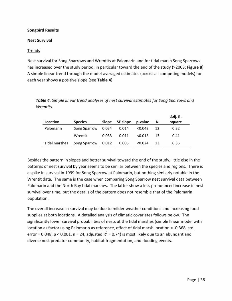
Songbird Results

Nest Survival

Trends

Nest survival for Song Sparrows and Wrentits at Palomarin and for tidal marsh Song Sparrows

has increased over the study period, in particular toward the end of the study (>2003; Figure 8).

A simple linear trend through the model‐averaged estimates (across all competing models) for

each year shows a positive slope (see Table 4).

Table 4. Simple linear trend analyses of nest survival estimates for Song Sparrows and

Wrentits.

Location Species Slope SE slope p‐value N Adj. R‐square

Palomarin Song Sparrow 0.034 0.014 <0.042 12 0.32

Wrentit 0.033 0.011 <0.015 13 0.41

Tidal marshes Song Sparrow 0.012 0.005 <0.024 13 0.35

Besides the pattern in slopes and better survival toward the end of the study, little else in the

patterns of nest survival by year seems to be similar between the species and regions. There is

a spike in survival in 1999 for Song Sparrow at Palomarin, but nothing similarly notable in the

Wrentit data. The same is the case when comparing Song Sparrow nest survival data between

Palomarin and the North Bay tidal marshes. The latter show a less pronounced increase in nest

survival over time, but the details of the pattern does not resemble that of the Palomarin

population.

The overall increase in survival may be due to milder weather conditions and increasing food

supplies at both locations. A detailed analysis of climatic covariates follows below. The

significantly lower survival probabilities of nests at the tidal marshes (simple linear model with

location as factor using Palomarin as reference, effect of tidal marsh location = ‐0.368, std.

error = 0.048, p < 0.001, n = 24, adjusted R2 = 0.74) is most likely due to an abundant and

diverse nest predator community, habitat fragmentation, and flooding events.

Figure 8. P

and Wrent

(standard e

model ave

Probability of n

tit (WREN) at P

errors) are the

raged predictio

est survival (1s

Palomarin and

e observed surv

ons.

st column) and

for Song Sparr

vival probabilit

d daily survival

row in tidal ma

ties; the line w

(2nd column)

arshes of the N

with the gray sh

for nests of So

North Bay. Dot

hade (standard

Page

ong Sparrow (S

s with error ba

d errors) shows

e | 39

SOSP)

ars

s the

Page | 40

These results suggest that management actions are not necessary at this time for Song

Sparrows and Wrentits at Palomarin. Had we detected the opposite pattern, a significant

decline in nest survival, research and management actions would be warranted. However, it is

important to consider breeding demographic parameters in addition to nest survival. For

example, Song Sparrows are significantly declining in abundance at Palomarin (PRBO,

unpublished data) which may warrant management actions that aim to increase their

populations.

Despite the encouraging trend, nest survival in the tidal marshes was very low. Management

actions should consider nest predator control in the short‐term and increasing the amount of

tidal marsh habitat in the short‐ to long‐term.

Effect of Bioyear Precipitation

We assumed that precipitation during the rainy season (measured as total October to March

precipitation and hereafter “bioyear” rainfall) would directly correlate with vegetation growth

and invertebrate abundance. The larger the growth, the better the year for nest survival, as

there would be more vegetative cover concealing the nests and perhaps greater food

availability.

Our hypothesis seems not to be supported by the data. Figure 9 shows a trend for Song

Sparrows and Wrentits at Palomarin, but it was not significant in any of the competing models

for these species at that location (see Appendix 2). The pattern of response was positive for

Song Sparrow and negative for Wrentit at Palomarin, and in the tidal marshes it was flat.

Despite the fact of its non‐significance, bioyear precipitation was present in competing models

for all species and locations, evidencing some role in nest survival.

These results are in agreement with prior estimates from Palomarin data (Chase et al. 2005),

who found a significant positive relationship between daily nest survival probabilities and the

quadratic of bioyear precipitation. Factors other than bioyear precipitation may be more

important in determining the survival of nests at Palomarin during the period we analyzed. This

may be the case if there is always high rainfall and small variations in vegetation growth have

little overall effect. For example, density‐dependent effects may be more important in driving

the survival of nests. Daily survival values are high for both the Song Sparrow and the Wrentit

during the period of this study. At the tidal marshes, the lack of suitable nesting vegetation

Page | 41

would diminish the effect of this variable. Thus, the lack of significant effects such as those

found by Chase et al. (2005) may be explained by climate differences between the periods

analyzed. Their dataset included 8 years of below‐average dry weather (6 of them below the

34‐year average), and years 1996 to 2000 had all high nest survival (see Figure 5 in Chase et al.

2005).

The apparent negative effect on Wrentits may also be explained by other factors with more

important influence on survival than those we considered, such as density‐dependent effects.

Nevertheless, the trend is in agreement with DeSante and Geupel’s (1987) report on low hatch‐

year counts after heavy bioyear rainfall.

The effect of bioyear precipitation may be more complex than just increasing vegetative cover

and productivity, or negative effects, as speculated by DeSante and Geupel (1987). Its effects

remain still unclear and more detailed studies will be required to properly provide management

recommendations. However, the contrast with the Chase et al. (2005) study seems to suggest

that drought may have a detrimental effect on survival.

Figure 9. E

Wrentit at

competing

Effect of total b

Palomarin and

g models for ea

bioyear precip

d at tidal mars

ach species and

itation on the

hes of the Nor

d location.

probability of

rth Bay. Graph

nest survival fo

hs show the mo

or nests of Son

odel‐averaged

Page

ng Sparrow and

effects from a

e | 42

d

all

Page | 43

Effect of Precipitation in Immediately Prior Months

We evaluated the effect of precipitation as a proxy variable for food availability, considering

total precipitation for the month prior to hatching, the total for the 2 prior months and 3 prior

months. We included only one of these variables per model, and these were not included in

models that also included bioyear precipitation. We hypothesized that an increase in

precipitation, represented by one of these precipitation parameters, may correlate with an

increase in food productivity and, thus, higher survival.

Only precipitation in the prior month was present in competing models for all three species and

locations, and it was a significant, but small effect in some competing models for the tidal

marsh Song Sparrows (Figure 10‐12). Precipitation in the three months prior to hatching

showed a significant effect in some of the competing models for the Wrentit at Palomarin. The

patterns at Palomarin for Song Sparrow and Wrentit are very similar to those of bioyear

precipitation. Overall, no discernible effects were observed at Palomarin that we could clearly

attribute to months immediately prior to hatching. Bioyear precipitation (see above) may

better account for increased productivity, the effect we sought to account for with these

parameters.

Precipitation during the prior three months for the tidal marsh Song Sparrow does show a

significant positive trend and opposite to that of bioyear, possibly suggesting increased food

productivity. Thus, the tidal marsh Song Sparrow’s nest survival may be favorable when there is

high late winter/early spring precipitation.

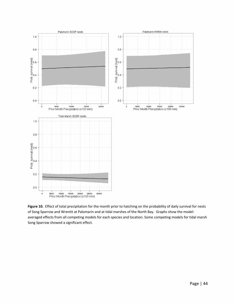
Figure 10.

of Song Sp

averaged e

Song Sparr

Effect of total

arrow and Wre

effects from all

row showed a

l precipitation

entit at Paloma

l competing m

significant effe

for the month

arin and at tida

odels for each

ect.

prior to hatch

al marshes of t

species and lo

hing on the pro

the North Bay.

ocation. Some

obability of dai

. Graphs show

competing mo

Page

ly survival for

w the model‐

odels for tidal m

e | 44

nests

marsh

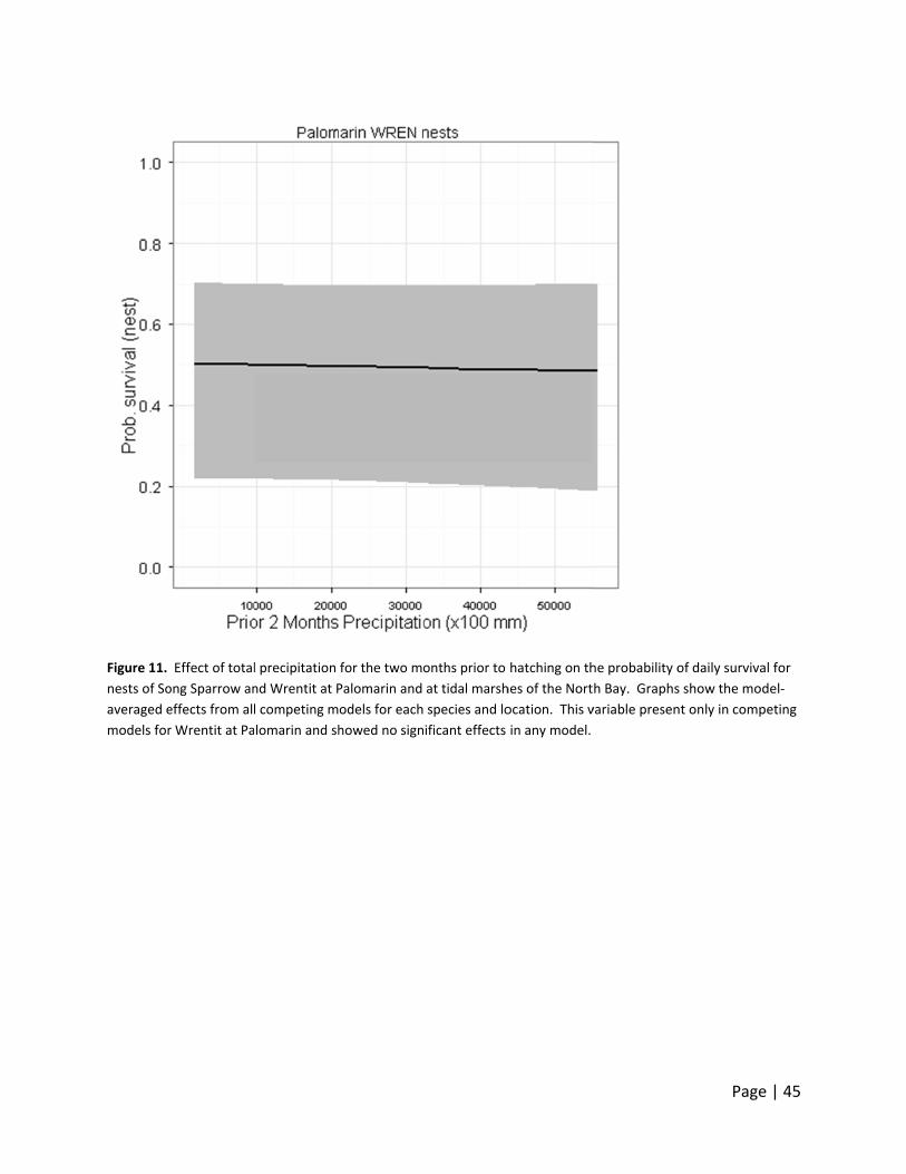
Figure 11.

nests of So

averaged e

models for

Effect of total

ong Sparrow an

effects from all

r Wrentit at Pa

l precipitation

nd Wrentit at P

l competing m

lomarin and sh

for the two mo

Palomarin and

odels for each

howed no sign

onths prior to

at tidal marsh

species and lo

ificant effects

hatching on th

hes of the Nort

ocation. This v

in any model.

he probability o

h Bay. Graphs

variable presen

Page

of daily surviva

s show the mod

nt only in comp

e | 45

al for

del‐

peting

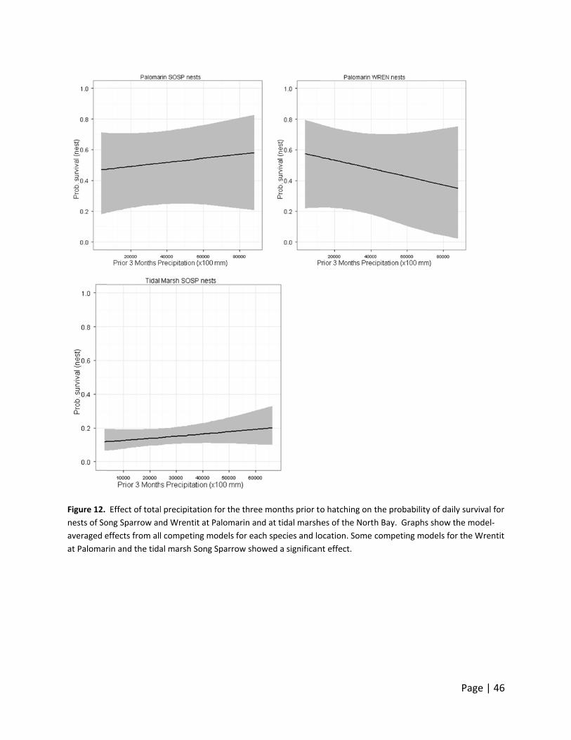
Figure 12.

nests of So

averaged e

at Palomar

Effect of total

ong Sparrow an

effects from all

rin and the tida

l precipitation

nd Wrentit at P

l competing m

al marsh Song

for the three m

Palomarin and

odels for each

Sparrow show

months prior to

at tidal marsh

species and lo

wed a significan

o hatching on

hes of the Nort

ocation. Some

nt effect.

the probability

h Bay. Graphs

competing mo

Page

y of daily surviv

s show the mod

odels for the W

e | 46

val for

del‐

Wrentit

Page | 47

Effect of Hatch‐Month Precipitation

We hypothesized that precipitation during the hatch month may have a detrimental effect on

survival of nests. We suspect that heavy rainfall may cause flooding of the tidal marshes, which

is an important cause of mortality and nest abandonment in our data. The effect of

precipitation at Palomarin is unclear. We included the variable in our analyses to see if there

was an effect of heavy rains during the hatching month, and it was selected among the

competing models for the Wrentit and tidal marsh Song Sparrow, but not for the Song Sparrow

at Palomarin.

Hatch‐month precipitation was among the variables in competing nest survival models for the

Wrentit at Palomarin and the Song Sparrow in tidal marshes. For Wrentits the overall effect

was positive, perhaps an indication of increased food productivity (Figure 13).

Notably, it had the hypothesized negative significant effects in some of the competing models

for tidal marsh Song Sparrow nest survival. This may be due to a possible correlation between

hatch‐month precipitation and flooding of the tidal marshes.

Figure 13.

at Palomar

models for

significant

Effect of total

rin and at tidal

r each species

effect.

l precipitation

marshes of th

and location. S

for the hatch‐

he North Bay. G

Some competin

month on the

Graphs show t

ng models for

probability of

the model‐aver

the tidal mars

daily survival f

raged effects f

h Song Sparrow

Page

for nests of Wr

from all compe

w showed a

e | 48

rentit

eting

Page | 49

Effects of Temperature

We evaluated the effects of minimum and maximum temperatures during the hatch month and

up to three months prior. We hypothesized that temperature (either or both monthly minima

and maxima) would positively correlate to food production and thus affect nest survival. Each

model, among the 73 evaluated, contained only one of the temperature variables, so only one

of them is present in each resulting competing model.

All temperature parameters were present in competing models for the species, but not all of

them in a single set of models for a species and location. Song Sparrows at Palomarin, for

example, included all but minimum temperature during the hatch month among its resulting

competing models. The minimum temperature on hatch month was present in competing

models for the Wrentit at Palomarin and the tidal marsh Song Sparrow, and it was a significant

effect in models in both cases. Additionally, competing models for the tidal marsh Song

Sparrow showed significant effects for minimum temperature for the two months prior to

hatching, maximum temperature during the hatch‐month, and maximum temperature on the

two and three months prior to hatching.

Notably, the data validates our hypothesis only for the Wrentit at Palomarin (Figure 14).

Temperature during the hatch month has an overall negative effect on Song Sparrow nest

survival, in particular in the tidal marshes. But it is important to note, too, that temperatures at

the tidal marshes vary nearly twice as widely as at Palomarin (maxima for the tidal marshes

vary from 15 to 30°C, whereas only 14 to 22°C at Palomarin), and the maxima (that correlate

with minima) may reflect high temperature stress for nesting Song Sparrows in the tidal

marshes. This thermal stress may be more important if there is no suitable vegetation cover, or

the individuals are under duress to reproduce in marginally suitable habitat, or both.

Figure 14.

for nests o

model‐ave

Wrentit at

some mod

Effect of mini

of Song Sparrow

eraged effects f

Palomarin and

els for the tida

mum and max

w and Wrentit

from all compe

d tidal marsh S

al marsh Song S

ximum tempera

at Palomarin a

eting models fo

Song Sparrow s

Sparrow show

ature for the h

and at tidal ma

or each species

showed a signi

ed a significan

hatch month o

arshes of the N

s and location

ficant effect of

nt effect of max

n the probabil

North Bay. Gra

. Some compe

f minimum tem

ximum temper

Page

ity of daily surv

aphs show the

eting models fo

mperature, and

rature.

e | 50

vival

or

d

Figure 15.

daily surviv

show the m

Effect of mini

val for nests of

model‐average

mum and max

f Song Sparrow

ed effects from

ximum tempera

w and Wrentit a

m all competing

ature for the m

at Palomarin a

g models for ea

month prior to

nd at tidal ma

ach species and

hatching on th

rshes of the No

d location.

Page

he probability

orth Bay. Grap

e | 51

of

phs

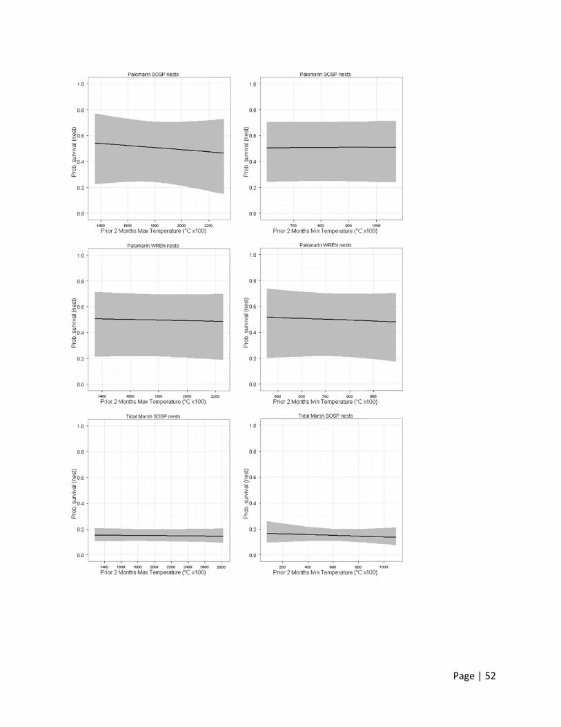
Page

e | 52

Page | 53

Figure 16. Effect of minimum and maximum temperature for the two months prior to hatching on the probability

of daily survival for nests of Song Sparrow and Wrentit at Palomarin and at tidal marshes of the North Bay. Graphs

show the model‐averaged effects from all competing models for each species and location. Some competing

models for the tidal marsh Song Sparrow showed a significant effect of minimum and maximum temperature.

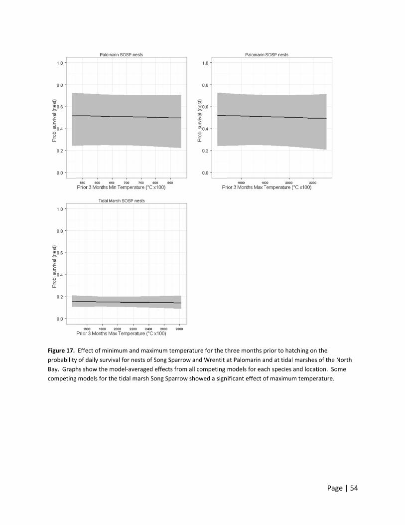
Figure 17.

probability

Bay. Grap

competing

Effect of mini

y of daily surviv

hs show the m

g models for th

mum and max

val for nests of

model‐averaged

e tidal marsh S

ximum tempera

f Song Sparrow

d effects from a

Song Sparrow

ature for the t

w and Wrentit a

all competing m

showed a sign

hree months p

at Palomarin a

models for eac

ificant effect o

prior to hatchin

nd at tidal ma

ch species and

of maximum te

Page

ng on the

rshes of the No

location. Som

emperature.

e | 54

orth

me

Page | 55

Date of First Arrival

Date of first arrival patterns show only significant trends for MacGillivray’s Warbler, Northern

Rough‐winged Swallow and Warbling Vireo (Figure 18 – regression lines shown only for those

species with a significant trend). Of these three species, only the Vireo has enough data to

properly assess a trend. The Warbling Vireo has been decreasing in abundance at Palomarin

(Gardali et al. 2000, Gardali and Jaramillo 2001), so the observed trend may be due to declining

numbers (Miller‐Rushing et al. 2008).

We attempted to fit the data to models that included total values for large‐scale climate indices

for all but one species (Northern Rough‐winged Swallow – the species had arrival date

estimates for <5 years). Below we report the fits for the resulting best model for each large‐

scale climate index and each species.

Significant relationships between large‐scale climate index variables and day of first arrival were

found for three Neotropical migrant species. Barn Swallow arrival data related negatively with

the cumulative monthly value of the Northern Oscillation Index. In particular, large negative

index values correlate with later arrival dates. The large negative index values are usually

associated with El Niño events and high upper ocean temperatures along the North American

west coast (Schwing et al. 2002). Therefore, the data seem to indicate later arrival dates during

El Niño event years.

Black‐headed Grosbeak arrival data show a negative correlation with ENSO values, but this is

mainly due to early arrival dates at index values >80. That is, the effect seems to be the

opposite of that observed in Barn Swallows: Black‐headed Grosbeak individuals tend to arrive

earlier during El Niño events. These events are characterized by higher surface temperatures in

the Northeastern Pacific.

The Pacific‐slope Flycatcher arrival data correlates negatively with the Pacific Decadal

Oscillation and positively with the Southern Oscillation Index. SOI values correlate with climate

patterns in the Tropical Southwestern Pacific that are not strongly related to Northeastern

Pacific weather (Schwing et al. 2001). This suggests possible effects at wintering grounds. The

PDO is largely an index of the North Pacific, with little relation to tropical patterns, and lasts

several decades, rather than months (Mantua et al. 1997). The data analyzed here are part of a

cooling PDO, which translates to colder North Pacific Sea temperatures. Together with the SOI

results, this suggests late arrivals during warmer years.

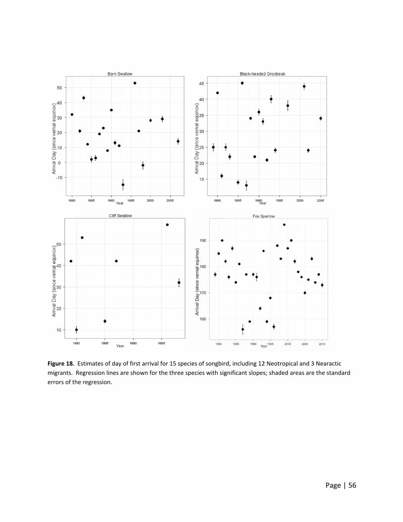
Figure 18.

migrants.

errors of th

Estimates of d

Regression lin

he regression.

day of first arri

es are shown f

val for 15 spec

for the three sp

cies of songbird

pecies with sig

d, including 12

gnificant slopes

2 Neotropical a

s; shaded area

Page

and 3 Nearactic

s are the stand

e | 56

c

dard

Figure 18 (

Nearactic m

standard e

(continued). E

migrants. Reg

errors of the re

Estimates of da

ression lines ar

gression.

ay of first arriva

re shown for th

al for 15 specie

he three specie

es of songbird,

es with signific

, including 12 N

cant slopes; sh

Page

Neotropical an

aded areas are

e | 57

d 3

e the

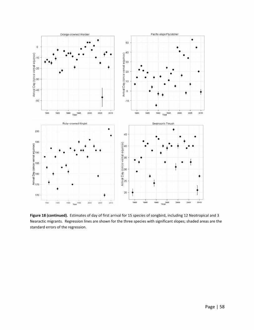
Figure 18 (

Nearactic m

standard e

(continued). E

migrants. Reg

errors of the re

Estimates of da

ression lines ar

gression.

ay of first arriva

re shown for th

al for 15 specie

he three specie

es of songbird,

es with signific

, including 12 N

cant slopes; sh

Page

Neotropical an

aded areas are

e | 58

d 3

e the

Figure 18 (

Nearactic m

standard e

(continued). E

migrants. Reg

errors of the re

Estimates of da

ression lines ar

gression.

ay of first arriva

re shown for th

al for 15 specie

he three specie

es of songbird,

es with signific

, including 12 N

cant slopes; sh

Page

Neotropical an

aded areas are

e | 59

d 3

e the

Figure 19.

indices (se

Swallow. S

Relationship b

e Climatic cova

Solid line is the

between day of

ariates and an

e cubic spline s

f first arrival an

alysis methods

smoother regre

nd best model

s above, and A

ession; shaded

fit variable va

Appendix, for m

d areas are the

lues from four

more details). R

standard erro

Page

r large‐scale cli

Results for Bar

ors of the regre

e | 60

mate

rn

ession.

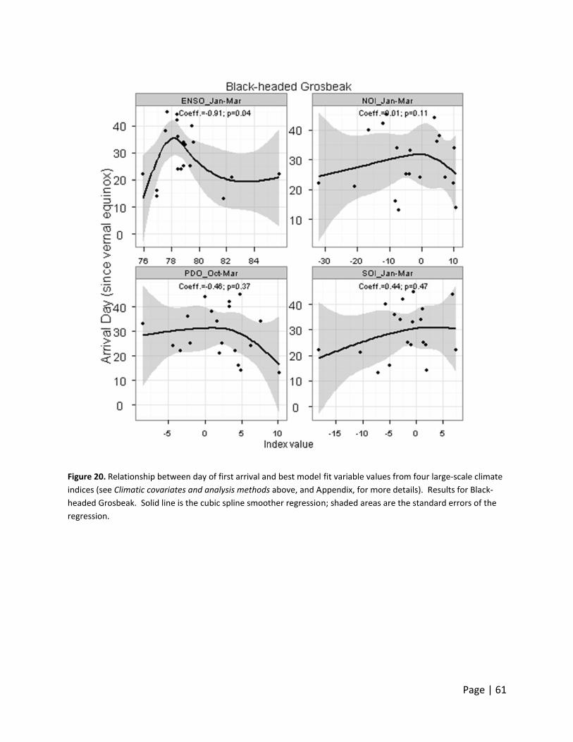
Figure 20.

indices (se

headed Gr

regression

Relationship b

e Climatic cova

rosbeak. Solid

.

between day of

ariates and an

line is the cub

f first arrival an

alysis methods

ic spline smoo

nd best model

s above, and A

ther regression

fit variable va

Appendix, for m

n; shaded area

lues from four

more details). R

as are the stan

Page

r large‐scale cli

Results for Blac

dard errors of

e | 61

mate

ck‐

the

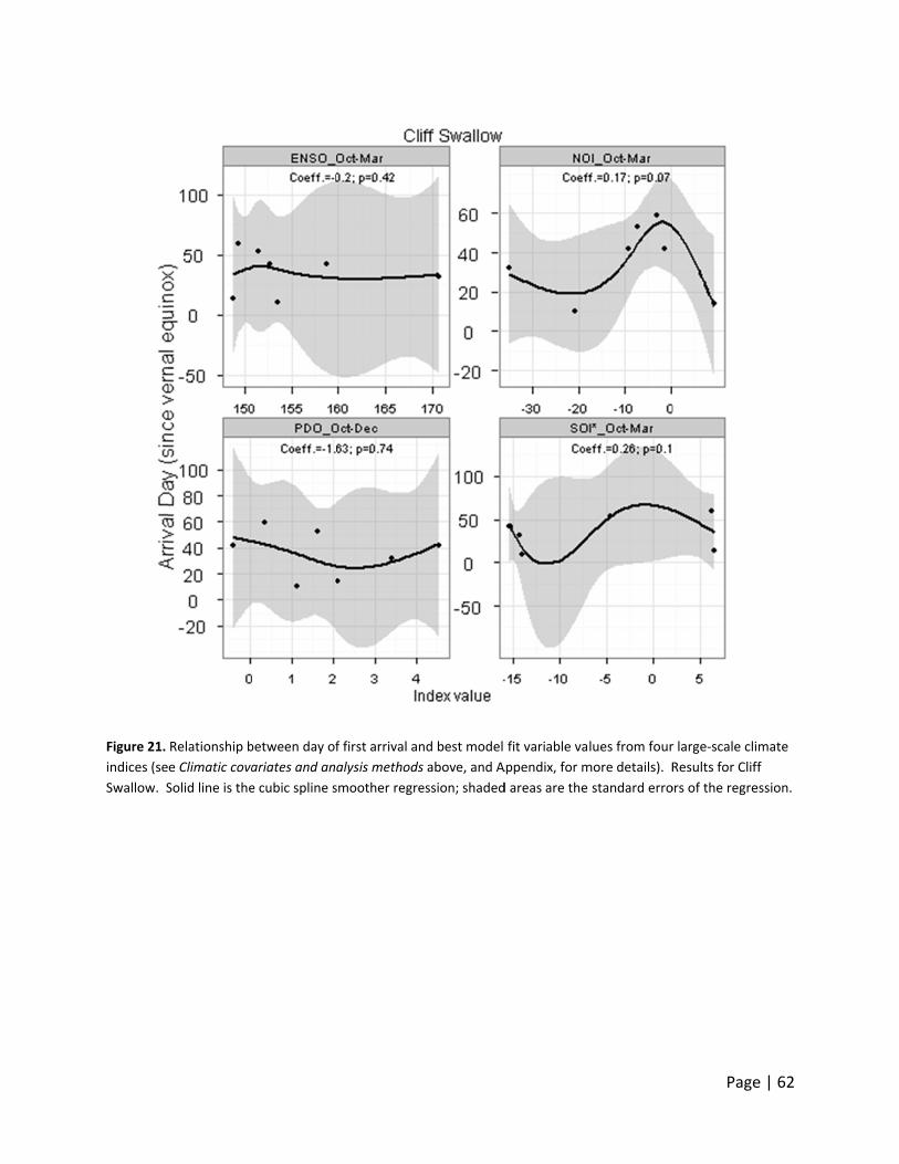
Figure 21.

indices (se

Swallow. S

Relationship b

e Climatic cova

Solid line is the

between day of

ariates and an

e cubic spline s

f first arrival an

alysis methods

smoother regre

nd best model

s above, and A

ession; shaded

fit variable va

Appendix, for m

d areas are the

lues from four

more details). R

standard erro

Page

r large‐scale cli

Results for Clif

ors of the regre

e | 62

mate

ff

ession.

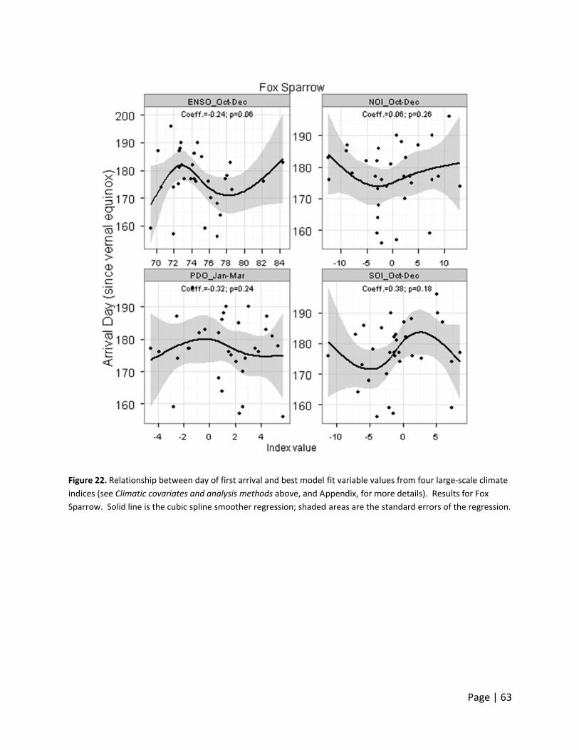
Figure 22.

indices (se

Sparrow. S

Relationship b

e Climatic cova

Solid line is the

between day of

ariates and an

e cubic spline s

f first arrival an

alysis methods

smoother regre

nd best model

s above, and A

ession; shaded

fit variable va

Appendix, for m

d areas are the

lues from four

more details). R

standard erro

Page

r large‐scale cli

Results for Fox

ors of the regre

e | 63

mate

x

ession.

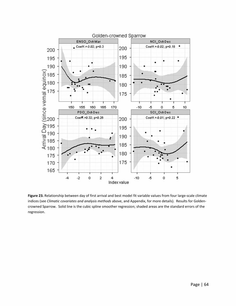
Figure 23.

indices (se

crowned S

regression

Relationship b

e Climatic cova

parrow. Solid

.

between day of

ariates and an

line is the cub

f first arrival an

alysis methods

ic spline smoo

nd best model

s above, and A

ther regressio

fit variable va

Appendix, for m

n; shaded area

lues from four

more details). R

as are the stan

Page

r large‐scale cli

Results for Gol

dard errors of

e | 64

mate

lden‐

the

Figure 24.

indices (se

MacGillivra

the regress

Relationship b

e Climatic cova

ay’s Warbler.

sion.

between day of

ariates and an

Solid line is the

f first arrival an

alysis methods

e cubic spline s

nd best model

s above, and A

smoother regre

fit variable va

Appendix, for m

ession; shaded

lues from four

more details). R

d areas are the

Page

r large‐scale cli

Results for

e standard erro

e | 65

mate

ors of

Figure 25.

indices (se

sided Flyca

regression

Relationship b

e Climatic cova

atcher. Solid li

.

between day of

ariates and an

ne is the cubic

f first arrival an

alysis methods

c spline smooth

nd best model

s above, and A

her regression;

fit variable va

Appendix, for m

; shaded areas

lues from four

more details). R

s are the stand

Page

r large‐scale cli

Results for Oliv

ard errors of th

e | 66

mate

ve‐

he

Figure 26.

indices (se

crowned W

regression

Relationship b

e Climatic cova

Warbler. Solid

.

between day of

ariates and an

line is the cub

f first arrival an

alysis methods

ic spline smoot

nd best model

s above, and A

ther regression

fit variable va

Appendix, for m

n; shaded area

lues from four

more details). R

as are the stan

Page

r large‐scale cli

Results for Ora

dard errors of

e | 67

mate

ange‐

the

Figure 27.

indices (se

slope Flyca

regression

Relationship b

e Climatic cova

atcher. Solid li

.

between day of

ariates and an

ne is the cubic

f first arrival an

alysis methods

c spline smooth

nd best model

s above, and A

her regression;

fit variable va

Appendix, for m

; shaded areas

lues from four

more details). R

s are the stand

Page

r large‐scale cli

Results for Pac

ard errors of th

e | 68

mate

cific‐

he

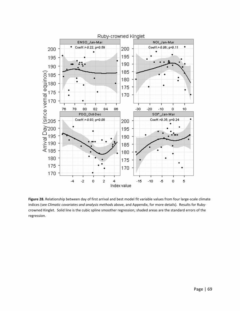
Figure 28.

indices (se

crowned K

regression

Relationship b

e Climatic cova

Kinglet. Solid li

.

between day of

ariates and an

ne is the cubic

f first arrival an

alysis methods

c spline smooth

nd best model

s above, and A

her regression;

fit variable va

Appendix, for m

; shaded areas

lues from four

more details). R

s are the stand

Page

r large‐scale cli

Results for Rub

ard errors of t

e | 69

mate

by‐

he

Figure 29.

indices (se

Swainson’s

regression

Relationship b

e Climatic cova

s Thrush. Solid

.

between day of

ariates and an

d line is the cub

f first arrival an

alysis methods

bic spline smoo

nd best model

s above, and A

other regressio

fit variable va

Appendix, for m

on; shaded are

lues from four

more details). R

eas are the stan

Page

r large‐scale cli

Results for

ndard errors o

e | 70

mate

f the

Figure 30.

indices (se

Vireo. Soli

Relationship b

e Climatic cova

id line is the cu

between day of

ariates and an

ubic spline smo

f first arrival an

alysis methods

oother regressi

nd best model

s above, and A

ion; shaded ar

fit variable va

Appendix, for m

eas are the sta

lues from four

more details). R

andard errors o

Page

r large‐scale cli

Results for Wa

of the regressio

e | 71

mate

arbling

on.

Figure 31.

indices (se

Warbler. S

Relationship b

e Climatic cova

olid line is the

between day of

ariates and an

cubic spline sm

f first arrival an

alysis methods

moother regre

nd best model

s above, and A

ssion; shaded

fit variable va

Appendix, for m

areas are the s

lues from four

more details). R

standard error

Page

r large‐scale cli

Results for Wil

rs of the regres

e | 72

mate

son’s

ssion.

Figure 32.

indices (se

Warbler. S

Relationship b

e Climatic cova

Solid line is the

between day of

ariates and an

e cubic spline s

f first arrival an

alysis methods

smoother regre

nd best model

s above, and A

ession; shaded

fit variable va

Appendix, for m

d areas are the

lues from four

more details). R

standard erro

Page

r large‐scale cli

Results for Yell

rs of the regre

e | 73

mate

low

ession.

Page | 74

Climate Projections

Waterfowl Results

By 2070, climate models project overall mean temperatures in the Central Valley to increase

anywhere from 3.1o – 4.3oF, and precipitation, although with much less certainty than

predictions for temperature, are expected to decrease by 1.9 – 6.9 inches (Snyder and Sloan

2005, PRBO Conservation Science 2011). Summer temperature spikes (heat waves) are likely to

become more common (PRBO Conservation Science 2011). Even under the most optimistic set

of changes suggested by these scenarios, in only 50 years, the effects we can predict to observe

in breeding waterfowl are significant. Below we present several projections for waterfowl

breeding parameters. In these cases, future projections of breeding parameters are model‐

averaged predictions of 1000 simulations, based on AICc weights of complete model set. Future

climate variables are estimated from climate scenarios based on a regional climate model

(RegCM3; Pal et al. 2007) as summarized in PRBO Conservation Science (2011). Given the high

uncertainty in future precipitation models as well as difficulty in determining when the

precipitation will occur, we only discuss results based on future temperatures.

Effects of Increased Temperature on Waterfowl Clutch Size

Assuming temperature trends will be consistent within all seasons, our models suggest that for

both Mallard and Gadwall, clutch sizes may decrease, especially for waterfowl nesting at Grizzly

Island Wildlife Area (Figure 33). Mean clutch size for Mallard nesting at Grizzly Island Wildlife

Area is projected to decrease by approximately 0.5 eggs, or 6%. For Gadwall, our models for

Grizzly Island Wildlife Area suggest that we will observe a decrease in mean clutch size for

Gadwall from 9.8 to 9.0‐9.2 eggs, representing a decrease in overall productivity of nearly 10%.

Relationship between clutch size and temperature is not as certain at Conaway Ranch. Although

our models for clutch size of Gadwall at Conaway Ranch showed a substantial negative

relationship with late spring temperatures (Figure 2), this was balanced by similar positive

relationship with summer and early spring temperatures. Final projections for Gadwall clutch

size (assuming comparable temperature increases in all seasons) suggest clutch size may

increase in the future for this later‐nesting duck species. However, clutch size models for

Gadwall nesting at Conaway Ranch, are based on a total of only 138 nests over 10 years. Clutch

size for Mallard nesting at Conaway Ranch, are not expected to change much at all.

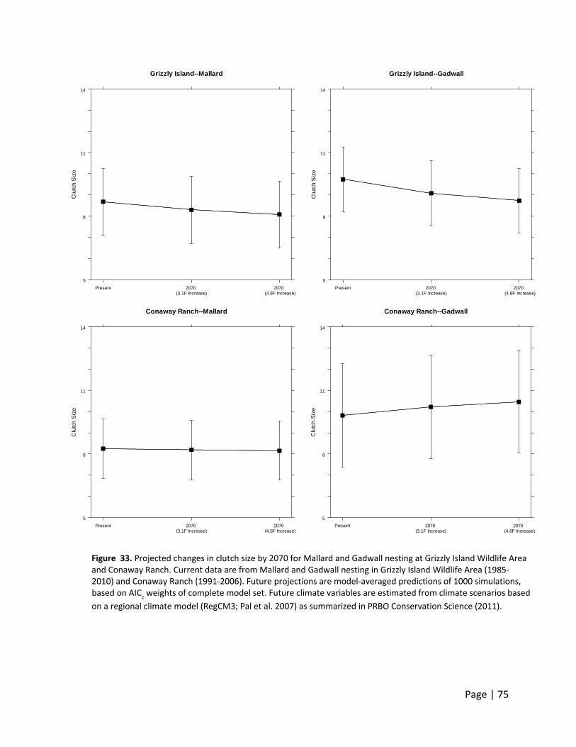
Page | 75

Figure 33. Projected changes in clutch size by 2070 for Mallard and Gadwall nesting at Grizzly Island Wildlife Area and Conaway Ranch. Current data are from Mallard and Gadwall nesting in Grizzly Island Wildlife Area (1985‐2010) and Conaway Ranch (1991‐2006). Future projections are model‐averaged predictions of 1000 simulations, based on AIC

c weights of complete model set. Future climate variables are estimated from climate scenarios based

on a regional climate model (RegCM3; Pal et al. 2007) as summarized in PRBO Conservation Science (2011).

Conaway Ranch--GadwallC

lutc

h S

ize

5

8

11

14

Present 2070 (3.1F Increase)



Clu

tch

Siz

e

5

8

11

14




Clu

tch

Siz

e

5

8

11

14



Grizzly Island--MallardC

lutc

h S

ize

5

8

11

14



Page | 76

Effects of Increased Temperature on Waterfowl Nesting Season Length

The length of the nesting season is a primary component in overall fecundity in nesting ducks.

Nest success, in general, is relatively low and a longer nesting season provides more

opportunities for waterfowl to renest. Dabbling ducks are known to renest several times in a

season if they lose their initial nesting attempts to predators. Conversely, a shorter nesting

season can dramatically reduce productivity if seasons become so short as to preclude

additional re‐nesting attempts. Our projections vary significantly among regions (Figure 34),

most likely a function of the fact that Grizzly Island Wildlife Area nesting season length may be

stabilized by the proximate location of the site to the San Francisco Bay. Instead, Conaway

Ranch as a habitat responds more directly to short‐term and seasonal weather conditions.

Looking more closely at Conaway Ranch where change in the nesting season is projected to be

more dramatic, suggests that the majority of change in the nesting season for Mallard will be a

result of a season that ends sooner than it currently does. In contrast, Gadwall appear to

benefit slightly from the warmer temperatures by nesting slightly earlier in the season (Figure

35).

Effects of Increased Temperature on Waterfowl Proportion of Eggs Hatched (Hatching Success)

As temperatures are expected to rise 3‐4oF over the next 50+ years, our models project that the

hatching success of both species at each site will decline (Figure 36). This result is especially

pronounced at Conaway Ranch, and presumably within the entire Central Valley where

temperatures can become extremely high within the cooling and stabilizing properties of the

San Francisco Bay and Coastal regions, such that Grizzly Island Wildlife Area experiences. Poor

hatching success may be manifested as a result of both direct egg mortality due to temperature

extremes, but it can also be caused by increased rates of abandonment and increased nest

recesses by females which would expose eggs to predation.

Page | 77

Grizzly Island--MallardC

en

tra

l sp

an

of A

ll N

est

Initi

atio

ns

0

17

33

50




Ce

ntr

al s

pa

n o

f All

Ne

st In

itia

tion

s

0

17

33

50




Ce

ntr

al s

pa

n o

f All

Ne

st In

itia

tion

s

0

17

33

50



Conaway Ranch--GadwallC

en

tra

l sp

an

of A

ll N

est

Initi

atio

ns

0

17

33

50



Figure 34. Projected changes in length of nesting season by 2070 for Mallard and Gadwall nesting in Grizzly Island Wildlife Area and Conaway Ranch. Current data are from Mallard and Gadwall nesting at Grizzly Island Wildlife Area (1985‐2010) and Conaway Ranch (1991‐2006). Future projections are model‐averaged predictions of 1000 simulations, based on AIC

c weights of complete model set. Future climate

variables are estimated from climate scenarios based on a regional climate model (RegCM3; Pal et al. 2007) as summarized in PRBO Conservation Science (2011).

Page | 78

Conaway Ranch--Mallard1

0th

Pe

rce

ntil

e o

f Ne

sts

Initi

ate

d

65

97

128

160




10

th P

erc

en

tile

of N

est

s In

itia

ted

65

97

128

160



Figure 35. Projected changes in the beginning (top row) and ending (bottom row) of the nesting season by 2070 for Mallard and Gadwall nesting at Grizzly Island Wildlife Area and Conaway Ranch. Current data are from Mallard and Gadwall nesting in Grizzly Island Wildlife Area (1985‐2010) and Conaway Ranch (1991‐2006). Future projections are model‐averaged predictions of 1000 simulations, based on AIC

c weights of complete model set.

Future climate variables are estimated from climate scenarios based on a regional climate model (RegCM3; Pal et al. 2007) as summarized in PRBO Conservation Science (2011).


90

th P

erc

en

tile

of N

est

s In

iitia

ted

120

137

153

170



Conaway Ranch--Gadwall9

0th

Pe

rce

ntil

e o

f Ne

sts

Iniit

iate

d

120

137

153

170



Page | 79

Grizzly Island--MallardP

rop

ort

ion

of E

gg

s H

atc

he

d

0

0.3

0.7

1




Pro

po

rtio

n o

f Eg

gs

Ha

tch

ed

0

0.3

0.7

1




Pro

po

rtio

n o

f Eg

gs

Ha

tch

ed

0

0.3

0.7

1



Conaway Ranch--GadwallP

rop

ort

ion

of E

gg

s H

atc

he

d

0

0.3

0.7

1



Figure 36. Projected changes in proportion of eggs hatching from a successful nest (hatching rate) by 2070 for Mallard and Gadwall nesting in Grizzly Island Wildlife Area and Conaway Ranch. Current data are from Mallard and Gadwall nesting at Grizzly Island Wildlife Area (1985‐2010) and Conaway Ranch (1991‐2006). Future projections are model‐averaged predictions of 1000 simulations, based on AIC

c weights of complete model set. Future climate

variables are estimated from climate scenarios based on a regional climate model (RegCM3; Pal et al. 2007) as summarized in PRBO Conservation Science (2011).

Page | 80

Songbird Results

Effects of Increased Temperature on Songbird Nest Survival

Future projections for the Song Sparrow and Wrentit suggest slightly enhanced nest survival. In

particular, the two projections we considered predict higher precipitation and higher

seasonality. This translates to more precipitation during the winter months and reduced

precipitation during the nesting months. Thus, any negative effects of hatch month

precipitation (especially important for tidal marsh Song Sparrow) may lessen in the future.

Similarly, more winter rains and warmer winter months may mean more vegetation growth,

increasing vegetation cover and productivity (especially important for the Palomarin Wrentit

population and the tidal marsh Song Sparrow).

The higher seasonality of the future climate models may translate into fewer hatch‐month rains

and fewer floods, resulting in higher survival. Sea level rise may cause higher competition for

higher nesting grounds, and higher chances of flooding for lower elevation sites (from high tides

or from little rainfall). Thus, the projected increase in survival may be inaccurate.

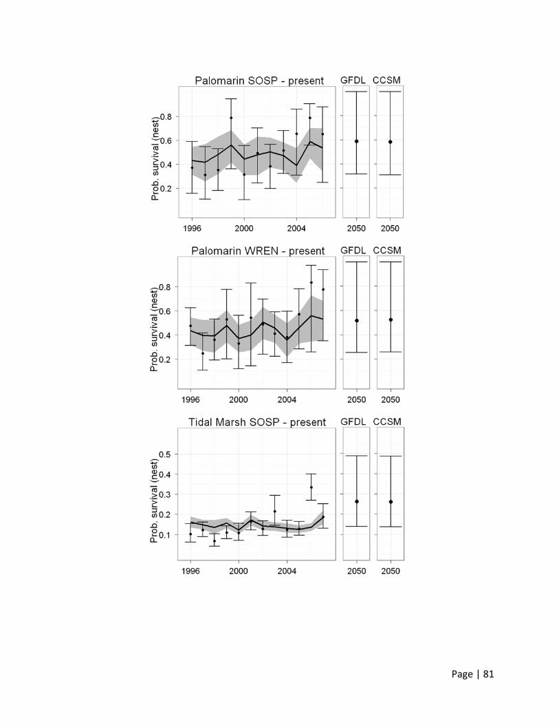
Page

e | 81

Page | 82

Figure 37. Projected nest survival probabilities for Song Sparrows and Wrentits at the Palomarin Research Station

and Song Sparrows in tidal marshes of the North Bay under climate scenario A2 of the IPCC as simulated by two

different global circulation models.

Management Implications

Waterfowl Nesting Demographics

The habitats in San Francisco Bay‐Delta (represented by Grizzly Island Wildlife Area) and the

Central Valley (represented by Conaway Ranch) are quite different, and it is not surprising that

waterfowl nesting demographics at these sites also are different. Waterfowl nesting within the

Grizzly Island Wildlife Area experience environmental conditions that are moderated by the San

Francisco Bay and proximity to the coast. There are substantial amounts of available water in

the area due to tidal sloughs and related wetlands. On the other hand, Conaway Ranch

presents nesting waterfowl with harsher environmental conditions, with little moderation of

temperatures by the bay and dependence on human land use for available water.

We found strong relationships between indices of successful nesting and temperature for both

Mallard and Gadwall at all sites. However, we expect that conditions in the future will become

more extreme in the Central Valley, as the area is projected to increase in temperature and the

frequency of extreme heat waves. Although there is no obvious way to directly reduce ambient

temperature, managers may have the ability to mitigate the effects that temperature has on

waterfowl nests. Our results suggest that, in addition to providing substantial amount of

quality nesting habitat, management efforts should aim to create habitat that minimizes

temperature that nests are exposed to. For example, nesting areas could contain significant

amounts of dense nesting cover that allow waterfowl to select nesting habitat that maximizes

the potential for shading, especially later in the nesting season. Management could include

using vegetation mixes that leave tall residual vegetation from prior nesting seasons while

vegetation grows during the current nesting season. This will be important in both the Central

Valley and San Francisco Bay‐Delta habitats, but we expect management actions to reduce heat

stress to be most effective in the Central Valley.

There is more uncertainty about future precipitation values, compared to future temperature

predictions. Nesting habitat in the Central Valley depends largely on spring rains and land use

practices (such as rice flooding) for available wetlands. It will be important for managers to

Page | 83

continue to consider habitat juxtaposition. Predators of duck nests, such as raccoons and

skunks, are known to select wetland and slough edges as preferred foraging routes (Greenwood

et al. 1999, Lariviere and Messier 2000, Phillips et al. 2004). Therefore, wetlands and sloughs

should not be located within upland duck nesting areas. However, nearby wetlands are

necessary as foraging areas for incubating females, and become especially important after eggs

hatch and females lead precocial ducklings to water within 24 hours of hatching. In general,

duckling survival does not decline with the distance they must travel to water, but wetlands

should be located within several miles of nesting habitat (Dzus and Clark 1997, Guyn and Clark

1999, Simpson et al. 2007). It should be a priority for managers to increase the availability of

both upland nesting habitat and summer wetlands (also known as reverse cycle wetlands) in

preferably large blocks of habitat. This will likely represent a significant challenge in the future

as land use practices change.

Our future research goals include investigating both the importance of nesting habitat and

larger landscape design (wetland adjacency) in more detail (e.g., Ackerman et al. 2009).

Research on the specific types of vegetation required (at both large and small scales), as well as

an estimate on the minimum threshold of wetland availability for successful breeding are

essential. Knowing where these wetlands should be located in relation to upland nesting

habitats will be key, as will understanding the small scale habitat structure and vegetation

requirements within upland nesting sites. Thus, while waterfowl do show a strong potential to

be negatively affected by future climate change scenarios, proactive management actions can

be taken to ameliorate some of these effects.

Songbird Nest Survival

Our results show that the relationship between nest survival and climate are complex and

poorly understood. The contrasts between Palomarin and tidal marsh Song Sparrow

populations sheds some light on potential stressors (temperature, limited adequate nesting

vegetation, possible density‐dependent mechanisms). The population at Palomarin seems to

be regulated by high density of breeders during periods of above‐average rainfall, as was the

case in our study, and by bioyear precipitation in periods of low rainfall, as may have been the

case of the Chase et al. (2005) study. This is a hypothesis that requires further and more

detailed studies.

Page | 84

Tidal marsh habitats of the North Bay have been extensively altered (Stralberg et al. 2010).

Populations of the subspecies of special concern Samuel’s and Suisun Song Sparrows may be

showing poor survival probabilities due to lack of appropriate nesting grounds. Spautz et al.

(2006) analyzed the abundance of Song Sparrows in the Bay tidal marshes and found that

vegetation composition and structure were important determinants. The lack of proper nesting

vegetation may cause higher susceptibility of the populations to the negative effects of high

temperature and high precipitation during the breeding season. The latter may correlate with

loss of nests due to flooding, which is an important cause of brood loss in our study.

Management alternatives may include means to reduce nest mortality due to flooding. Spautz

et al. (2006) discuss recommendations to enhance habitats for Song Sparrows, including

protection of a mosaic of tidal marsh habitats.

Songbird Arrival Phenology and Large‐Scale Climate Indices

The relationship between the day of arrival of Neotropical and Nearctic migrants and global

climatic variables is unclear. The large‐scale climate indices may be interpreted as single‐

parameter indicators of large‐scale climate processes, but the indices do not capture the

entirety of the processes they summarize, and the effect of these processes on the biota is far

from clear. We were interested in identifying indicators of change in global climate that would

act as cues to the timing of departure from wintering or breeding grounds, and arrival at

Palomarin.

Our results suggest that for species such as the Barn Swallow will show later arrival dates during

El Niño event years, while species such as the Black‐headed Grosbeak will arrive earlier. These

patterns must be understood better. Species such as the Pacific‐slope Flycatcher seem to arrive

later during warmer years. The timing of arrival may have important consequences if it is linked

to the availability of resources at the breeding grounds. Arrival past the peak of availability of

important nesting resources may result in reduced productivity (Both et al. 2006).

Little can be done locally to mitigate the effects of mismatches between timing of arrival and

blooming of important nesting resources for local populations. However, knowledge of these

potential effects may prompt range‐wide and international actions to reduce the negative

impacts on the populations. For example, the timing mismatch may vary throughout the range

(because of spatial heterogeneity of nesting resources), or other stressors such as predators or

sub‐optimal nesting habitats may be restored to reduce negative impacts where possible.

Page | 85

Literature Cited

Ackerman, J. T. 2002. Of mice and Mallards: positive indirect effects of coexisting prey on waterfowl nest success. Oikos 99:469–480.

Ackerman, J. T., J. M. Eadie, D. L. Loughman, G. S. Yarris, and M. R. McLandress. 2003a. The influence of partial clutch depredation on duckling production. Journal of Wildlife Management 67:576–587.

Ackerman, J. T., and J. M. Eadie. 2003b. Current versus future reproduction: an experimental test of parental investment decisions using nest desertion by Mallards (Anas platyrhynchos). Behavioral Ecology and Sociobiology 54:264–273.

Ackerman, J. T., J. M. Eadie, G. S. Yarris, D. L. Loughman, and M. R. McLandress. 2003c. Cues for investment: nest desertion in response to partial clutch depredation in dabbling ducks. Animal Behaviour 66:871–883.

Ackerman, J. T., A. L. Blackmer, and J. M. Eadie. 2004. Is predation on waterfowl nests density dependent? Tests at three spatial scales. Oikos 107:128–140.

Ackerman, J. T., J. M. Eadie, and T. G. Moore. 2006. Does life history predict risk‐taking behavior of wintering dabbling ducks? Condor 108:530‐546.

Ackerman, J. T., J. Kwolek, R. Eddings, D. Loughman, and J. Messerli. 2009. Evaluating upland habitat management at the Grizzly Island Wildlife Area: effects on dabbling duck nest density and nest success. Administrative Report, U. S. Geological Survey, Western Ecological Research Center, Davis, CA and California Waterfowl Association, Sacramento, CA; 26 pp.

Arcese, P., M. K. Sogge, A. B. Marr and M. A. Patten. 2002. Song Sparrow (Melospiza melodia), The Birds of North America Online (A. Poole, Ed.). Ithaca: Cornell Lab of Ornithology; Retrieved from the Birds of North America Online: http://bna.birds.cornell.edu.bnaproxy.birds.cornell.edu/bna/species/704 (doi:10.2173/bna.704)

Bellrose, F. C. 1980. Ducks, Geese, and Swans of North America, 3rd Edition. Stackpole Books, Harrisburg, PA. 540 pp.

Both, C., S. Bouwhuis, C. M. Lessells, and M . E. Visser. 2006. Climate change and population declines in a long‐distance migratory bird. Nature 441:81‐83; doi:10.1038/nature04539.

Page | 86

Burnham, K. P., and D. R. Anderson. 2002. Model Selection and Multi‐Model Inference: A Practical Information‐Theoretic Approach. Springer Verlag.

Chase, M. K. 2001. Reproductive Success, Natal Dispersal, and Recruitment in a Song Sparrow (Melospiza melodia) Population Breeding in California Coastal Scrub. Ph.D. dissertation, University of California ‐ Riverside.

Chase, M. K. 2002. Nest site selection and nest success in a Song Sparrow population: the significance of spatial variation. Condor 104:103‐116.

Chase M. K., Nur N., and G. R. Geupel. 2005. Effects of weather and population density on reproductive success and population dynamics in a Song Sparrow (Melospiza melodia) population: A long‐term study. Auk 122:571‐592.

DeSante, D.F., and G.R. Geupel. 1987. Landbird productivity in central coastal California: the relationship to annual rainfall and a reproductive failure in 1986. The Condor 89(3):636‐653.

Dzus, E. H., and R. G. Clark. 1997. Overland travel, food abundance, and wetland use by Mallards: relationships with offspring survival. Wilson Bulletin 109:504‐515.

Gardali, T. and A. Jaramillo. 2001. Further evidence for a population decline in the western Warbling Vireo. Western Birds 32:173‐176.

Gardali, T., G. Ballard, N. Nur, and G.R. Geupel. 2000. Demography of a declining population of warbling vireos in coastal California. The Condor 102:601‐609.

Gelman, A., and J. Hill. 2007. Data Analysis Using Regression and Multilevel/Hierarchical Models. Cambridge University Press.

Gelman, A., J.B. Carlin, H.S. Stern, and D.B. Rubin. Bayesian Data Analysis, 2nd Edition. Chapman & Hall/CRC. Boca Raton, FL. 668 pp.

Geupel, G. R., and G. Ballard. 2002. Wrentit (Chamaea fasciata), The Birds of North America Online (A. Poole, Ed.). Ithaca: Cornell Lab of Ornithology; Retrieved from the Birds of North America Online: http://bna.birds.cornell.edu.bnaproxy.birds.cornell.edu/bna/species/654 (doi:10.2173/bna.654)

Gordo, O. 2007. Why are bird migration dates shifting? A review of weather and climate effects on avian migratory phenology. Climate Research 35: 37‐58.

Page | 87

Gordon, A. D. 1999. Classification. 2nd edition. London: Chapman & Hall/CRC. Boca Raton, FL. 256 pp.

Greenwood, R. J., A. B. Sargeant, J. L. Piehl, D. A. Buhl, and B. A. Hanson. 1999. Foods and foraging of prairie striped skunks during the avian nesting season. Wildlife Society Bulletin 27:823‐832.

Guyn, K. L., and R. G. Clark. 1999. Factors affecting survival of Northern Pintail ducklings in Alberta. Condor 101:369‐377.

Herzog, M. P. 2011. Nestsurvival package (version 0.51) for R statistical programming language. Currently available via email: [email protected]

Humple, D., and G. R. Geupel. 2004. Song Sparrow (Melospiza melodia). In The Riparian Bird Conservation Plan: a strategy for reversing the decline of riparian‐associated birds in California. California Partners in Flight. http://www.prbo.org/calpif/htmldocs/riparian_v‐2.html (accessed May 2011).

Johnson, D. H. 1979. Estimating nest success: The Mayfield Method and an alternative. Auk 96(4):651‐661.

Jongsomjit D., S. L. Jones, T. Gardali, G. R. Geupel, and P. J. Gouse. 2007. A guide to nestling development and aging in altricial passerines. U.S. Department of Interior, Fish and Wildlife Service, Biological Technical Publication, FWS/BTP‐R6008‐2007, Washington, D.C.

Keeling, T. 2009. Modified JMA ENSO Index and Its Improvements to ENSO Classification, M.S. Thesis, Florida State University, Tallahassee, FL, USA.

Lariviere, S., and F. Messier. 2000. Habitat selection and use of edges by striped skunks in the Canadian prairies. Canadian Journal of Zoology 78:366‐372.

MacMynowsky, D. P., T. L . Root, G. Ballard, and G. R. Geupel. 2007. Changes in spring arrival of Nearctic‐Neotropical migrants attributed to multiscalar climate. Global Change Biology 13:1‐13, doi: 10.1111/j.1365‐2486.2007.01448.x

Mantua, N. J., and S. R. Hare, Y. Zhang, J. M. Wallace, and R. C. Francis. 1997: A Pacific interdecadal climate oscillation with impacts on salmon production. Bulletin of the American Meteorological Society, 78: 1069‐1079.

Page | 88

Martin, T.E., and G.R. Geupel. 1993. Nest‐monitoring plots: methods for locating nests and monitoring success. Journal of Field Ornithology 64(4):507‐519.

Mayfield, H. F. 1961. Nest success calculated from exposure. Wilson Bulletin 73:255‐261.

Mayfield, H. F. 1975. Suggestions for calculating nest success. Wilson Bulletin 87:456‐466.

McLandress, M. R., G. S. Yarris, A. H. Perkins, D. P. Connelly, and D. G. Raveling. 1996. Nesting biology of Mallards in California. Journal of Wildlife Management 60(1): 94‐107.

Miller‐Rushing, A., T. L. Lloyd‐Evans, R. B. Primack, and P. Satzinger. 2008. Bird migration times, climate change, and changing population sizes. Global Change Biology 14: 1959‐1972, doi: 10.1111/j.1365‐2486.2008.01619.x

Pal, J. S. and coauthors. 2007. Regional climate modeling for the developing world: The ICTP RegCMS and RegCNET. Bulletin of the American Meteorological Society 88:1395‐1409. DOI: 10.1175/BAMS‐88‐9‐1395

Pinheiro, J.C. and D.M. Bates. 2000. Mixed‐effects models in S and S‐plus. Springer. New York. 528 pp.

Phillips, M. L., W. R. Clark, S. M. Nusser, M. A. Sovada, and R. J. Greenwood. 2004. Analysis of predator movements in prairie landscapes with contrasting grassland composition. Journal of Mammalogy 85:187‐195.

PRBO Conservation Science. 2011. Projected Effects of Climate Change in California: Ecoregional Summaries Emphasizing Consequences for Wildlife. Version 1.0. http://data.prbo.org/apps/bssc/

PRISM Climate Group, Oregon State University, http://prism.oregonstate.edu. Data downloaded April 2011.

R Development Core Team. 2011. R: A language and environment for statistical computing. R Foundation for Statistical Computing, Vienna, Austria. ISBN 3‐900051‐07‐0, URL: http://www.R‐project.org

Ralph, C. J., G. R. Geupel, P. Pyle, T. E. Martin, and D. F. DeSante. 1993. Handbook of field methods for monitoring landbirds. U.S. Department of Agriculture General Technical Report PSW‐GTR‐144.

Page | 89

Robinson, R. A., S. R. Baillie, and H. Q. P. Crick. 2007. Weather‐dependent survival: implications of climate change for passerine population processes. Ibis 149:357‐364.

Sagarin, R. 2001. False estimates of advance of spring. Nature 414: 600.

Seavy, N., K. E. Dybala and M. A. Snyder. 2008. Climate Models and Ornithology. The Auk 125:1‐10.

Shaffer, T. L. 2004. A unified approach to analyzing nest success. Auk 121:526‐540.

Silkey, M., N. Nur, and G.R. Geupel. 1999. The use of mist‐net capture rates to monitor annual variation in abundance: a validation study. Condor 101:288‐298.

Simpson J. W., T. Yerkes, T. D. Nudds, B. D. Smith. 2007. Effects of habitat on mallard duckling survival in the Great Lakes region. Journal of Wildlife Management 71:1885‐1891.

Snyder, M. A., and L. C. Sloan 2005. Transient future climate over the western U.S. using a regional climate model. Earth Interactions. Vol. 9, Paper 11.

Spautz, H., N. Nur, D. Stralberg, and Y. Chan. 2006. Multiple‐scale habitat relationships of tidal‐marsh breeding birds in the San Francisco Bay estuary. Studies in Avian Biology 32: 247‐269.

Stralberg, D., D. Jongsomjit, C. A. Howell, M. A. Snyder, J. D. Alexander, et al. 2009. Re‐Shuffling of Species with Climate Disruption: A No‐Analog Future for California Birds? PLoS ONE 4(9): e6825. doi:10.1371/journal.pone.0006825

Stralberg, D., M. P. Herzog, N. Nur, K. A. Tuxen, and M. Kelly. 2010. Predicting Avian Abundance Within and Across Tidal Marshes Using Fine‐Scale Vegetation and Geomorphic Metrics. Wetlands 30: 475‐487, doi:10.1007/s13157‐010‐0052‐8

Schwing, F. B., T. Murphree, and P. M. Green. 2002. The Northern Oscillation Index: A new climate index for the northeast Pacific. Progress in Oceanography 53:115‐139.

Van Turnhout, C. A. M., R. P. B. Foppen, R. S. E. W. Leuwen, A. Van Strien, and H. Siepel. 2010. Life‐history and ecological correlates of population change in Dutch breeding birds. Biological Conservation 143:173‐181.

Venables, W. N. and B. D. Ripley. 2002. Modern applied statistics with S. 4th Edition. Springer. New York. 495 pp.

Page | 90

Wright, L. J., R. A. Hoblyn, R. E. Green, C. G. R. Bowden, J. W. Mallord, W. J. Sutherland, and P. M. Dolman. 2009. Importance of climatic and environmental change in the demography of a multi‐brooded passerine, the Woodlark Lullula arborea. Journal of Animal Ecology 78:1191‐1202.

Page | 91

Appendix 1. Definitions and naming conventions for variables used in models.

Variable Definition

mean.Tmean.late.winter mean daily mean temperature in late winter mean.Tmean.early.spring mean daily mean temperature in early spring mean.Tmean.late.spring mean daily mean temperature in late spring mean.Tmean.early.summer mean daily mean temperature in early summer max.Tmax.late.spring maximum daily maximum temperature in late spring max.Tmax.early.summer maximum daily maximum temperature in early summer sum.Prcp.late.winter cumulative precipitation in late winter sum.Prcp.early.spring cumulative precipitation in early spring sum.Prcp.late.spring cumulative precipitation in late spring sum.Prcp.early.summer cumulative precipitation in early summer count.extreme.high.95.Tmax number of days where the maximum temperature exceeded 95°F

within a specific interval of time mean.Tmean mean daily mean temperature within a specific interval of time max.Tmax maximum daily maximum temperature within a specific interval of

time sum.Prcp. cumulative precipitation within a specific interval of time initdate.julian initiation date of individual nest measured in days since January 1 date date at mean of interval nest age age of nest at middle of interval age when nest was found estimated age of nest when it was first discovered relative initiation date initiation date of nest, relative to the 10th percentile of all nests in

a given year (initiation date ‐ 10th‐percentile.initationdate) year year of study site nesting field

Page | 92

Appendix 2. Summary of model candidate sets*.

Analyses performed on Site Level Averages Analyses performed on Individual Nests

Covariate

10th Percentile of Nest Initiation

Dates

90th Percentile of Nest Initiation

Dates

Central Span of Breeding Season

Clutch Size

Initiation Date


Nest Survival

mean.Tmean.late.winter ‐ ‐ X ‐ X ‐ ‐ mean.Tmean.early.spring X X X X X ‐ ‐ mean.Tmean.late.spring X X X X X X ‐ mean.Tmean.early.summer ‐ X X X ‐ X ‐ max.Tmax.late.spring ‐ ‐ ‐ ‐ ‐ X ‐ max.Tmax.early.summer ‐ ‐ ‐ ‐ ‐ X ‐ sum.Prcp.late.winter X X X X X ‐ ‐ sum.Prcp.early.spring X X X X X ‐ ‐ sum.Prcp.late.spring X X X X X ‐ ‐ sum.Prcp.early.summer ‐ X X X ‐ X ‐ count.extreme.high.95.Tmax ‐ ‐ ‐ ‐ ‐ X X** mean.Tmean ‐ ‐ ‐ ‐ ‐ ‐ X** max.Tmax ‐ ‐ ‐ ‐ ‐ ‐ X** sum.Prcp ‐ ‐ ‐ ‐ ‐ ‐ X** initiation.date ‐ ‐ ‐ X ‐ ‐ ‐ date ‐ ‐ ‐ ‐ ‐ ‐ X (date)2 ‐ ‐ ‐ ‐ ‐ ‐ X nest age ‐ ‐ ‐ ‐ ‐ ‐ X (nest age)2 ‐ ‐ ‐ ‐ ‐ ‐ X age when nest was found ‐ ‐ ‐ ‐ ‐ ‐ X (age when nest was found)2 ‐ ‐ ‐ ‐ ‐ ‐ X relative initation date ‐ ‐ ‐ ‐ ‐ ‐ X (relative initiation date)2 ‐ ‐ ‐ ‐ ‐ ‐ X year (factor) Random Random Random Random Random Random X site (factor) Random Random Random Random Random Random ‐ * See Appendix 1 for variable definitions ** including all 2‐way interactions among these covariates

Page | 93

Appendix 3. Variables in competing models for songbirds’ nest survival analyses.

Variable Song Sparrow Palomarin

Wrentit Palomarin

Song Sparrow Tidal

Marshes

Nest age (at middle of exposure interval) X* X* X*

(Nest age)2 X* X* X*

(Nest age)3 X* X*

Day since first initiation date of the season X X X*

(Day since first initiation date of the season)2 X X X*

(Day since first initiation date of the season)3 X X X*

Year (factor) X* X* X*

Precipitation October‐March X X X Total precipitation on hatch month X X* Total precipitation on prior month X X X* Total precipitiation on prior 2 months X Total precipitation on prior 3 months X* X* Min. temperature on hatch month X* X*

Min. temperature on prior month X X

Min. temperature on prior 2 months X X X* Min. temperature on prior 3 months X Max. temperature on hatch month X X*

Max. temperature on prior month X X

Max. temperature on prior 2 months X X X* Max. temperature on prior 3 months X X*

Number of competing models 14 10 12

Asterisks (*) indicate significant contributions to model fits (p‐value < 0.05).

Page | 94

Appendix 4. Model selection tables for waterfowl clutch size, nest initiation date, 10th percentile of nest

initiation dates, central span of nests initiated, 90th percentile of nest initiation dates, proportion of eggs

hatched, and nest survival.

All models, except nest survival models included site and year as random effects. See Appendix 1 for definitions of all

variables used in models.

Only models with AICc<=3.0 are provided within these tables. Please refer to Appendix 2 for a list of all the models run for a

given demographic parameter.

Variable importance is presented for all parameters where variable importance was >= 0.5

Page | 95

Clutch Size

Mallard at Grizzly Island Wildlife Area

Model Selection Table

Model K AICc ΔAICc Weight

clutchsize ~ mean.Tmean.late.spring + mean.Tmean.early.summer + initdate.julian 6 18953.16 0.00 0.07 clutchsize ~ mean.Tmean.late.spring + initdate.julian 5 18953.86 0.70 0.05 clutchsize ~ mean.Tmean.late.spring + sum.Prcp.early.summer + mean.Tmean.early.summer + initdate.julian 7 18954.36 1.20 0.04 clutchsize ~ sum.Prcp.late.winter + mean.Tmean.late.spring + mean.Tmean.early.summer + initdate.julian 7 18954.85 1.69 0.03 clutchsize ~ mean.Tmean.late.spring + sum.Prcp.early.summer + initdate.julian 6 18954.89 1.73 0.03 clutchsize ~ sum.Prcp.early.spring + mean.Tmean.late.spring + mean.Tmean.early.summer + initdate.julian 7 18955.10 1.94 0.03 clutchsize ~ mean.Tmean.early.spring + mean.Tmean.late.spring + mean.Tmean.early.summer + initdate.julian 7 18955.12 1.96 0.03 clutchsize ~ sum.Prcp.late.spring + mean.Tmean.late.spring + mean.Tmean.early.summer + initdate.julian 7 18955.16 2.00 0.02 clutchsize ~ sum.Prcp.late.winter + mean.Tmean.late.spring + sum.Prcp.early.summer + mean.Tmean.early.summer + initdate.julian 8 18955.42 2.26 0.02 clutchsize ~ sum.Prcp.early.spring + mean.Tmean.late.spring + initdate.julian 6 18955.43 2.27 0.02 clutchsize ~ mean.Tmean.early.summer + initdate.julian 5 18955.46 2.30 0.02 clutchsize ~ mean.Tmean.early.spring + mean.Tmean.late.spring + initdate.julian 6 18955.61 2.45 0.02 clutchsize ~ sum.Prcp.late.winter + mean.Tmean.late.spring + initdate.julian 6 18955.70 2.54 0.02 clutchsize ~ sum.Prcp.late.spring + mean.Tmean.late.spring + initdate.julian 6 18955.82 2.66 0.02 clutchsize ~ sum.Prcp.late.spring + mean.Tmean.early.summer + initdate.julian 6 18955.99 2.83 0.02

Page | 96

Variable Importance

Variable Variable

Importance

Model‐averaged Coefficient

initdate.julian 1.000 ‐0.038mean.Tmean.late.spring 0.709 ‐0.049mean.Tmean.early.summer 0.621 ‐0.065

Page | 97

Mallard at Conaway Ranch

Model Selection


clutchsize ~ sum.Prcp.late.winter + mean.Tmean.early.spring + mean.Tmean.late.spring + sum.Prcp.early.summer + initdate.julian 8 2104.72 0.00 0.11 clutchsize ~ sum.Prcp.late.winter + sum.Prcp.early.spring + mean.Tmean.early.spring + mean.Tmean.late.spring + sum.Prcp.early.summer + initdate.julian 9 2106.41 1.68 0.05 clutchsize ~ mean.Tmean.early.spring + mean.Tmean.late.spring + sum.Prcp.early.summer + initdate.julian 7 2106.74 2.02 0.04 clutchsize ~ sum.Prcp.late.winter + mean.Tmean.early.spring + sum.Prcp.late.spring + mean.Tmean.late.spring + sum.Prcp.early.summer + initdate.julian 9 2106.74 2.02 0.04 clutchsize ~ sum.Prcp.late.winter + mean.Tmean.early.spring + mean.Tmean.late.spring + sum.Prcp.early.summer + mean.Tmean.early.summer + initdate.julian 9 2106.75 2.03 0.04 clutchsize ~ mean.Tmean.early.spring + sum.Prcp.late.spring + mean.Tmean.late.spring + sum.Prcp.early.summer + initdate.julian 8 2107.51 2.79 0.03

Variable Importance

Variable Variable

Importance


initdate.julian 1.00 ‐0.03sum.Prcp.early.summer 0.66 0.44mean.Tmean.early.spring 0.65 ‐0.08sum.Prcp.late.winter 0.62 0.02mean.Tmean.late.spring 0.61 0.06

Page | 98

Gadwall at Grizzly Island Wildlife Area

Model Selection


clutchsize ~ sum.Prcp.early.spring + mean.Tmean.early.spring + sum.Prcp.late.spring + mean.Tmean.late.spring + initdate.julian

8 4929.27 0.00 0.11

clutchsize ~ sum.Prcp.early.spring + mean.Tmean.early.spring + sum.Prcp.late.spring + mean.Tmean.late.spring + sum.Prcp.early.summer + initdate.julian

9 4930.51 1.24 0.06

clutchsize ~ mean.Tmean.early.spring + sum.Prcp.late.spring + mean.Tmean.late.spring + mean.Tmean.early.summer + initdate.julian

8 4931.02 1.75 0.05

clutchsize ~ sum.Prcp.early.spring + mean.Tmean.early.spring + sum.Prcp.late.spring + mean.Tmean.late.spring + mean.Tmean.early.summer + initdate.julian

9 4931.07 1.80 0.04

clutchsize ~ sum.Prcp.late.winter + sum.Prcp.early.spring + mean.Tmean.early.spring + sum.Prcp.late.spring + mean.Tmean.late.spring + initdate.julian

9 4931.12 1.85 0.04

clutchsize ~ mean.Tmean.early.spring + sum.Prcp.late.spring + mean.Tmean.late.spring + initdate.julian 7 4931.28 2.01 0.04 clutchsize ~ sum.Prcp.late.winter + sum.Prcp.early.spring + mean.Tmean.early.spring + sum.Prcp.late.spring + mean.Tmean.late.spring + sum.Prcp.early.summer + initdate.julian

10 4931.93 2.66 0.03

clutchsize ~ sum.Prcp.early.spring + mean.Tmean.early.spring + mean.Tmean.late.spring + initdate.julian 7 4932.16 2.89 0.03 clutchsize ~ mean.Tmean.early.spring + mean.Tmean.late.spring + mean.Tmean.early.summer + initdate.julian

7 4932.25 2.98 0.02

clutchsize ~ sum.Prcp.early.spring + mean.Tmean.early.spring + sum.Prcp.late.spring + mean.Tmean.late.spring + sum.Prcp.early.summer + mean.Tmean.early.summer + initdate.julian

10 4932.27 3.00 0.02

clutchsize ~ mean.Tmean.early.spring + sum.Prcp.late.spring + mean.Tmean.late.spring + sum.Prcp.early.summer + mean.Tmean.early.summer + initdate.julian

9 4932.27 3.00 0.02

Page | 99

Variable Importance

Variable Variable

Importance


initdate.julian 1.00 ‐0.05mean.Tmean.early.spring 0.86 ‐0.11mean.Tmean.late.spring 0.82 ‐0.07sum.Prcp.late.spring 0.69 ‐0.08sum.Prcp.early.spring 0.58 0.02

Page | 100

Gadwall at Conaway Ranch

Model Selection


clutchsize ~ sum.Prcp.early.spring + mean.Tmean.early.spring + sum.Prcp.late.spring + mean.Tmean.late.spring + sum.Prcp.early.summer + mean.Tmean.early.summer + initdate.julian

10 348.32 0.00 0.30

clutchsize ~ mean.Tmean.early.spring + sum.Prcp.late.spring + mean.Tmean.late.spring + sum.Prcp.early.summer + mean.Tmean.early.summer + initdate.julian

9 348.74 0.42 0.24

clutchsize ~ sum.Prcp.late.winter + mean.Tmean.early.spring + sum.Prcp.late.spring + mean.Tmean.late.spring + sum.Prcp.early.summer + mean.Tmean.early.summer + initdate.julian

10 349.54 1.23 0.16

clutchsize ~ sum.Prcp.late.winter + sum.Prcp.early.spring + mean.Tmean.early.spring + sum.Prcp.late.spring + mean.Tmean.late.spring + sum.Prcp.early.summer + mean.Tmean.early.summer + initdate.julian

11 350.33 2.01 0.11

Variable Importance

Variable Variable

Importance


mean.Tmean.late.spring 0.99 ‐1.12initdate.julian 0.98 ‐0.03mean.Tmean.early.summer 0.94 0.79sum.Prcp.early.summer 0.90 ‐3.16mean.Tmean.early.spring 0.90 0.47

Page | 101

sum.Prcp.late.spring 0.90 ‐1.20

Page | 102

Nest Initiation Date


Model Selection


initdate.julian ~ mean.Tmean.late.winter + mean.Tmean.early.spring + sum.Prcp.late.spring + mean.Tmean.late.spring

7 90801.72 0.00 0.22

initdate.julian ~ mean.Tmean.late.winter + sum.Prcp.early.spring + mean.Tmean.early.spring + sum.Prcp.late.spring + mean.Tmean.late.spring

8 90803.58 1.85 0.09

initdate.julian ~ sum.Prcp.late.winter + mean.Tmean.late.winter + mean.Tmean.early.spring + sum.Prcp.late.spring + mean.Tmean.late.spring

8 90803.62 1.90 0.08

initdate.julian ~ mean.Tmean.late.winter + mean.Tmean.early.spring + mean.Tmean.late.spring 6 90803.97 2.25 0.07 initdate.julian ~ mean.Tmean.late.winter + sum.Prcp.late.spring + mean.Tmean.late.spring 6 90804.27 2.55 0.06 initdate.julian ~ mean.Tmean.late.winter + mean.Tmean.late.spring 5 90804.68 2.96 0.05

Variable Importance

Variable Variable

Importance


mean.Tmean.late.spring 0.93 ‐1.94mean.Tmean.late.winter 0.84 1.93mean.Tmean.early.spring 0.67 ‐1.28sum.Prcp.late.spring 0.60 ‐1.41

Page | 103


Model Selection


initdate.julian ~ sum.Prcp.late.winter + mean.Tmean.late.winter + mean.Tmean.early.spring 6 8223.65 0.00 0.09 initdate.julian ~ sum.Prcp.late.winter + mean.Tmean.late.winter 5 8223.85 0.20 0.08 initdate.julian ~ sum.Prcp.late.winter + mean.Tmean.late.winter + mean.Tmean.early.spring + sum.Prcp.late.spring

7 8224.53 0.88 0.06

initdate.julian ~ sum.Prcp.late.winter + mean.Tmean.late.winter + mean.Tmean.early.spring + mean.Tmean.late.spring

7 8225.14 1.49 0.04

initdate.julian ~ sum.Prcp.late.winter + mean.Tmean.late.winter + sum.Prcp.early.spring + mean.Tmean.early.spring

7 8225.32 1.67 0.04

initdate.julian ~ 1 3 8225.47 1.82 0.04 initdate.julian ~ sum.Prcp.late.winter + mean.Tmean.late.winter + mean.Tmean.late.spring 6 8225.79 2.14 0.03 initdate.julian ~ sum.Prcp.late.winter + mean.Tmean.late.winter + sum.Prcp.early.spring 6 8225.85 2.20 0.03 initdate.julian ~ sum.Prcp.late.winter + mean.Tmean.late.winter + sum.Prcp.late.spring 6 8225.86 2.21 0.03 initdate.julian ~ mean.Tmean.late.winter + mean.Tmean.early.spring 5 8226.03 2.39 0.03 initdate.julian ~ mean.Tmean.late.winter 4 8226.38 2.73 0.02 initdate.julian ~ sum.Prcp.late.winter 4 8226.46 2.81 0.02 initdate.julian ~ mean.Tmean.early.spring 4 8226.48 2.83 0.02 initdate.julian ~ sum.Prcp.late.winter + mean.Tmean.late.winter + sum.Prcp.early.spring + mean.Tmean.early.spring + sum.Prcp.late.spring

8 8226.51 2.86 0.02

initdate.julian ~ sum.Prcp.late.winter + mean.Tmean.late.winter + mean.Tmean.early.spring + sum.Prcp.late.spring + mean.Tmean.late.spring

8 8226.57 2.92 0.02

initdate.julian ~ sum.Prcp.late.spring 4 8226.60 2.95 0.02

Page | 104

Variable Importance

Variable Variable

Importance


mean.Tmean.late.winter 0.68 1.62sum.Prcp.late.winter 0.65 ‐0.53mean.Tmean.early.spring 0.52 ‐0.77

Page | 105


Model Selection


initdate.julian ~ mean.Tmean.late.winter + mean.Tmean.early.spring + mean.Tmean.late.spring 6 19250.75 0.00 0.07 initdate.julian ~ mean.Tmean.late.winter + mean.Tmean.late.spring 5 19251.25 0.50 0.05 initdate.julian ~ mean.Tmean.late.winter + mean.Tmean.early.spring 5 19251.32 0.57 0.05 initdate.julian ~ mean.Tmean.late.spring 4 19251.47 0.72 0.05 initdate.julian ~ mean.Tmean.late.winter + mean.Tmean.early.spring + sum.Prcp.late.spring + mean.Tmean.late.spring

7 19251.56 0.81 0.05

initdate.julian ~ sum.Prcp.late.winter + mean.Tmean.late.winter + mean.Tmean.early.spring 6 19252.09 1.34 0.04 initdate.julian ~ sum.Prcp.late.winter + mean.Tmean.early.spring 5 19252.25 1.50 0.03 initdate.julian ~ sum.Prcp.late.winter + mean.Tmean.late.winter + mean.Tmean.early.spring + mean.Tmean.late.spring

7 19252.34 1.60 0.03

initdate.julian ~ sum.Prcp.late.winter + mean.Tmean.late.spring 5 19252.44 1.70 0.03 initdate.julian ~ mean.Tmean.late.winter + sum.Prcp.early.spring + mean.Tmean.early.spring + mean.Tmean.late.spring

7 19252.64 1.89 0.03

initdate.julian ~ mean.Tmean.late.winter + sum.Prcp.late.spring + mean.Tmean.late.spring 6 19252.75 2.00 0.03 initdate.julian ~ mean.Tmean.late.winter + sum.Prcp.early.spring + mean.Tmean.early.spring 6 19252.80 2.05 0.02 initdate.julian ~ sum.Prcp.late.winter + mean.Tmean.early.spring + mean.Tmean.late.spring 6 19252.80 2.05 0.02 initdate.julian ~ sum.Prcp.late.winter + mean.Tmean.late.winter + sum.Prcp.early.spring + mean.Tmean.early.spring

7 19252.97 2.22 0.02

initdate.julian ~ sum.Prcp.late.winter + sum.Prcp.early.spring + mean.Tmean.early.spring 6 19253.11 2.36 0.02 initdate.julian ~ mean.Tmean.early.spring + mean.Tmean.late.spring 5 19253.19 2.44 0.02 initdate.julian ~ mean.Tmean.late.winter + sum.Prcp.early.spring + mean.Tmean.late.spring 6 19253.24 2.49 0.02 initdate.julian ~ sum.Prcp.late.winter + mean.Tmean.late.winter + mean.Tmean.late.spring 6 19253.24 2.50 0.02 initdate.julian ~ sum.Prcp.late.winter + mean.Tmean.late.winter + mean.Tmean.early.spring + 8 19253.25 2.50 0.02

Page | 106

sum.Prcp.late.spring + mean.Tmean.late.spring initdate.julian ~ mean.Tmean.late.winter + sum.Prcp.early.spring + mean.Tmean.early.spring + sum.Prcp.late.spring + mean.Tmean.late.spring

8 19253.27 2.52 0.02

initdate.julian ~ mean.Tmean.late.winter + mean.Tmean.early.spring + sum.Prcp.late.spring 6 19253.31 2.56 0.02 initdate.julian ~ sum.Prcp.late.spring + mean.Tmean.late.spring 5 19253.43 2.68 0.02 initdate.julian ~ sum.Prcp.early.spring + mean.Tmean.late.spring 5 19253.47 2.72 0.02

Variable Importance

Variable Variable

Importance


mean.Tmean.late.spring 0.62 ‐0.68mean.Tmean.early.spring 0.61 ‐1.02mean.Tmean.late.winter 0.60 0.84

Page | 107


Model Selection


initdate.julian ~ 1 + (1 | site) + (1 | year) 3 1247.88 0.00 0.14 initdate.julian ~ mean.Tmean.early.spring + (1 | site) + (1 | year) 4 1249.37 1.49 0.07 initdate.julian ~ sum.Prcp.late.winter + (1 | site) + (1 | year) 4 1249.75 1.87 0.05 initdate.julian ~ sum.Prcp.late.spring + (1 | site) + (1 | year) 4 1249.90 2.02 0.05 initdate.julian ~ mean.Tmean.late.spring + (1 | site) + (1 | year) 4 1249.90 2.02 0.05 initdate.julian ~ sum.Prcp.early.spring + (1 | site) + (1 | year) 4 1249.96 2.08 0.05 initdate.julian ~ mean.Tmean.late.winter + (1 | site) + (1 | year) 4 1249.98 2.09 0.05 initdate.julian ~ mean.Tmean.early.spring + mean.Tmean.late.spring + (1 | site) + (1 | year) 5 1250.81 2.93 0.03

Variable Importance

No variables in model set with Variable Importance > 0.5

Page | 108

10th Percentile of Nest Initiation Dates


Model Selection


nest.initdate.lower10 ~ sum.Prcp.late.winter + mean.Tmean.early.spring + sum.Prcp.late.spring + mean.Tmean.late.spring

7 2574.71 0.00 0.09

nest.initdate.lower10 ~ mean.Tmean.early.spring + mean.Tmean.late.spring 5 2575.12 0.41 0.08 nest.initdate.lower10 ~ mean.Tmean.early.spring + sum.Prcp.late.spring + mean.Tmean.late.spring 6 2575.18 0.48 0.07 nest.initdate.lower10 ~ sum.Prcp.late.spring + mean.Tmean.late.spring 5 2575.29 0.58 0.07 nest.initdate.lower10 ~ sum.Prcp.late.winter + mean.Tmean.early.spring 5 2575.39 0.68 0.07 nest.initdate.lower10 ~ mean.Tmean.late.spring 4 2575.52 0.81 0.06 nest.initdate.lower10 ~ sum.Prcp.late.winter + mean.Tmean.early.spring + mean.Tmean.late.spring 6 2575.85 1.14 0.05 nest.initdate.lower10 ~ sum.Prcp.early.spring + mean.Tmean.early.spring + mean.Tmean.late.spring 6 2575.93 1.22 0.05 nest.initdate.lower10 ~ sum.Prcp.early.spring + mean.Tmean.early.spring + sum.Prcp.late.spring + mean.Tmean.late.spring

7 2576.02 1.31 0.05

nest.initdate.lower10 ~ sum.Prcp.early.spring + sum.Prcp.late.spring + mean.Tmean.late.spring 6 2576.05 1.34 0.05 nest.initdate.lower10 ~ mean.Tmean.early.spring 4 2576.06 1.35 0.05 nest.initdate.lower10 ~ sum.Prcp.early.spring + mean.Tmean.late.spring 5 2576.24 1.53 0.04 nest.initdate.lower10 ~ sum.Prcp.late.winter + sum.Prcp.early.spring + mean.Tmean.early.spring + sum.Prcp.late.spring + mean.Tmean.late.spring

8 2576.50 1.80 0.04

nest.initdate.lower10 ~ sum.Prcp.late.winter + mean.Tmean.early.spring + sum.Prcp.late.spring 6 2576.89 2.18 0.03 nest.initdate.lower10 ~ sum.Prcp.late.winter + sum.Prcp.late.spring + mean.Tmean.late.spring 6 2577.08 2.37 0.03 nest.initdate.lower10 ~ sum.Prcp.late.winter + sum.Prcp.early.spring + mean.Tmean.early.spring + mean.Tmean.late.spring

7 2577.37 2.66 0.02

nest.initdate.lower10 ~ sum.Prcp.late.winter + sum.Prcp.early.spring + mean.Tmean.early.spring 6 2577.42 2.72 0.02

Page | 109

nest.initdate.lower10 ~ sum.Prcp.late.winter + mean.Tmean.late.spring 5 2577.57 2.86 0.02

Variable Importance

Variable Variable

Importance


mean.Tmean.late.spring 0.76 ‐1.41mean.Tmean.early.spring 0.68 ‐1.52

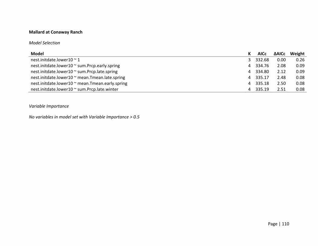
Page | 110


Model Selection


nest.initdate.lower10 ~ 1 3 332.68 0.00 0.26 nest.initdate.lower10 ~ sum.Prcp.early.spring 4 334.76 2.08 0.09 nest.initdate.lower10 ~ sum.Prcp.late.spring 4 334.80 2.12 0.09 nest.initdate.lower10 ~ mean.Tmean.late.spring 4 335.17 2.48 0.08 nest.initdate.lower10 ~ mean.Tmean.early.spring 4 335.18 2.50 0.08 nest.initdate.lower10 ~ sum.Prcp.late.winter 4 335.19 2.51 0.08

Variable Importance


Page | 111


Model Selection


nest.initdate.lower10 ~ 1 3 2320.23 0.00 0.14 nest.initdate.lower10 ~ mean.Tmean.late.spring 4 2320.56 0.33 0.12 nest.initdate.lower10 ~ mean.Tmean.early.spring 4 2321.76 1.54 0.06 nest.initdate.lower10 ~ sum.Prcp.late.winter 4 2321.87 1.64 0.06 nest.initdate.lower10 ~ sum.Prcp.late.spring + mean.Tmean.late.spring 5 2322.06 1.83 0.05 nest.initdate.lower10 ~ sum.Prcp.late.spring 4 2322.24 2.02 0.05 nest.initdate.lower10 ~ sum.Prcp.early.spring 4 2322.24 2.02 0.05 nest.initdate.lower10 ~ sum.Prcp.late.winter + mean.Tmean.late.spring 5 2322.40 2.17 0.05 nest.initdate.lower10 ~ mean.Tmean.early.spring + mean.Tmean.late.spring 5 2322.56 2.33 0.04 nest.initdate.lower10 ~ sum.Prcp.early.spring + mean.Tmean.late.spring 5 2322.61 2.38 0.04 nest.initdate.lower10 ~ sum.Prcp.late.winter + mean.Tmean.early.spring 5 2322.71 2.49 0.04

Variable Importance


Page | 112


Model Selection


nest.initdate.lower10 ~ mean.Tmean.early.spring 4 202.10 0.00 0.23 nest.initdate.lower10 ~ 1 3 202.79 0.69 0.17 nest.initdate.lower10 ~ sum.Prcp.late.winter 4 204.07 1.97 0.09 nest.initdate.lower10 ~ mean.Tmean.early.spring + mean.Tmean.late.spring 5 204.64 2.54 0.07 nest.initdate.lower10 ~ sum.Prcp.late.winter + mean.Tmean.early.spring 5 204.74 2.64 0.06

Variable Importance

Variable Variable

Importance


mean.Tmean.early.spring 0.52 ‐1.57

Page | 113

Central Span Nesting Season


Model Selection


nestingseason.centralspan ~ sum.Prcp.early.spring + sum.Prcp.late.spring + sum.Prcp.early.summer 6 2647.69 0.00 0.05 nestingseason.centralspan ~ sum.Prcp.late.spring + sum.Prcp.early.summer 5 2647.76 0.07 0.05 nestingseason.centralspan ~ sum.Prcp.early.spring + mean.Tmean.early.spring + sum.Prcp.late.spring + sum.Prcp.early.summer

7 2649.37 1.68 0.02

nestingseason.centralspan ~ sum.Prcp.early.spring + sum.Prcp.late.spring + sum.Prcp.early.summer + mean.Tmean.early.summer

7 2649.40 1.71 0.02

nestingseason.centralspan ~ sum.Prcp.late.spring 4 2649.41 1.72 0.02 nestingseason.centralspan ~ sum.Prcp.early.spring + sum.Prcp.late.spring + mean.Tmean.late.spring + sum.Prcp.early.summer

7 2649.42 1.72 0.02

nestingseason.centralspan ~ mean.Tmean.late.winter + sum.Prcp.late.spring + sum.Prcp.early.summer 6 2649.48 1.79 0.02 nestingseason.centralspan ~ mean.Tmean.early.spring + sum.Prcp.late.spring + sum.Prcp.early.summer 6 2649.51 1.82 0.02 nestingseason.centralspan ~ sum.Prcp.late.winter + sum.Prcp.early.spring + sum.Prcp.late.spring + sum.Prcp.early.summer

7 2649.60 1.91 0.02

nestingseason.centralspan ~ mean.Tmean.late.winter + sum.Prcp.early.spring + sum.Prcp.late.spring + sum.Prcp.early.summer

7 2649.65 1.96 0.02

nestingseason.centralspan ~ sum.Prcp.late.spring + mean.Tmean.late.spring + sum.Prcp.early.summer 6 2649.71 2.02 0.02 nestingseason.centralspan ~ sum.Prcp.late.spring + sum.Prcp.early.summer + mean.Tmean.early.summer 6 2649.72 2.03 0.02 nestingseason.centralspan ~ sum.Prcp.late.winter + sum.Prcp.late.spring + sum.Prcp.early.summer 6 2649.82 2.13 0.02 nestingseason.centralspan ~ sum.Prcp.early.spring + sum.Prcp.late.spring 5 2649.89 2.20 0.02 nestingseason.centralspan ~ mean.Tmean.late.winter + mean.Tmean.early.spring + sum.Prcp.late.spring + sum.Prcp.early.summer

7 2650.24 2.55 0.01

Page | 114

nestingseason.centralspan ~ mean.Tmean.late.winter + sum.Prcp.early.spring + mean.Tmean.early.spring + sum.Prcp.late.spring + sum.Prcp.early.summer

8 2650.61 2.91 0.01

nestingseason.centralspan ~ mean.Tmean.early.spring + sum.Prcp.late.spring 5 2650.64 2.95 0.01

Variable Importance

Variable Variable

Importance


sum.Prcp.late.spring 0.85 1.75sum.Prcp.early.summer 0.65 4.93sum.Prcp.early.spring 0.52 0.25

Page | 115


Model Selection


nestingseason.centralspan ~ mean.Tmean.early.summer 4 341.09 0.00 0.06 nestingseason.centralspan ~ 1 3 341.32 0.23 0.05 nestingseason.centralspan ~ mean.Tmean.late.winter 4 341.76 0.67 0.04 nestingseason.centralspan ~ sum.Prcp.early.spring 4 342.45 1.35 0.03 nestingseason.centralspan ~ sum.Prcp.late.spring + mean.Tmean.early.summer 5 342.82 1.72 0.03 nestingseason.centralspan ~ mean.Tmean.late.winter + sum.Prcp.late.spring 5 342.89 1.80 0.02 nestingseason.centralspan ~ sum.Prcp.early.spring + mean.Tmean.early.summer 5 343.05 1.96 0.02 nestingseason.centralspan ~ mean.Tmean.late.winter + sum.Prcp.late.spring + mean.Tmean.late.spring 6 343.30 2.21 0.02 nestingseason.centralspan ~ mean.Tmean.late.winter + sum.Prcp.early.spring 5 343.55 2.45 0.02 nestingseason.centralspan ~ mean.Tmean.late.winter + mean.Tmean.early.summer 5 343.55 2.45 0.02 nestingseason.centralspan ~ sum.Prcp.early.summer + mean.Tmean.early.summer 5 343.59 2.50 0.02 nestingseason.centralspan ~ mean.Tmean.early.spring 4 343.61 2.52 0.02 nestingseason.centralspan ~ mean.Tmean.early.spring + mean.Tmean.early.summer 5 343.64 2.55 0.02 nestingseason.centralspan ~ sum.Prcp.late.winter + mean.Tmean.early.summer 5 343.67 2.58 0.02 nestingseason.centralspan ~ mean.Tmean.late.spring 4 343.72 2.62 0.02 nestingseason.centralspan ~ mean.Tmean.late.spring + mean.Tmean.early.summer 5 343.76 2.66 0.02 nestingseason.centralspan ~ sum.Prcp.late.winter 4 343.76 2.67 0.02 nestingseason.centralspan ~ sum.Prcp.early.summer 4 343.80 2.71 0.02 nestingseason.centralspan ~ sum.Prcp.late.spring 4 343.83 2.73 0.02 nestingseason.centralspan ~ sum.Prcp.late.winter + mean.Tmean.late.winter 5 344.06 2.97 0.01

Variable Importance


Page | 116


Model Selection


nestingseason.centralspan ~ sum.Prcp.late.winter + sum.Prcp.early.spring + mean.Tmean.early.spring 6 2405.76 0.00 0.08 nestingseason.centralspan ~ sum.Prcp.late.winter + sum.Prcp.early.spring + mean.Tmean.early.spring + sum.Prcp.late.spring

7 2406.89 1.13 0.05

nestingseason.centralspan ~ sum.Prcp.late.winter + sum.Prcp.early.spring + mean.Tmean.early.spring + mean.Tmean.early.summer

7 2407.56 1.80 0.03

nestingseason.centralspan ~ sum.Prcp.late.winter + sum.Prcp.early.spring + mean.Tmean.early.spring + sum.Prcp.early.summer

7 2407.64 1.88 0.03

nestingseason.centralspan ~ sum.Prcp.late.winter + mean.Tmean.early.spring + sum.Prcp.late.spring 6 2407.71 1.95 0.03 nestingseason.centralspan ~ sum.Prcp.late.winter + mean.Tmean.late.winter + sum.Prcp.early.spring + mean.Tmean.early.spring

7 2407.82 2.06 0.03

nestingseason.centralspan ~ sum.Prcp.late.winter + mean.Tmean.early.spring 5 2407.83 2.07 0.03 nestingseason.centralspan ~ sum.Prcp.late.winter + sum.Prcp.early.spring + mean.Tmean.early.spring + mean.Tmean.late.spring

7 2407.84 2.08 0.03

nestingseason.centralspan ~ sum.Prcp.late.winter + sum.Prcp.early.spring + mean.Tmean.early.spring + sum.Prcp.late.spring + mean.Tmean.late.spring

8 2408.49 2.73 0.02

nestingseason.centralspan ~ sum.Prcp.late.winter + sum.Prcp.early.spring + mean.Tmean.early.spring + sum.Prcp.late.spring + mean.Tmean.early.summer

8 2408.62 2.86 0.02

nestingseason.centralspan ~ sum.Prcp.late.winter + sum.Prcp.late.spring 5 2408.70 2.94 0.02

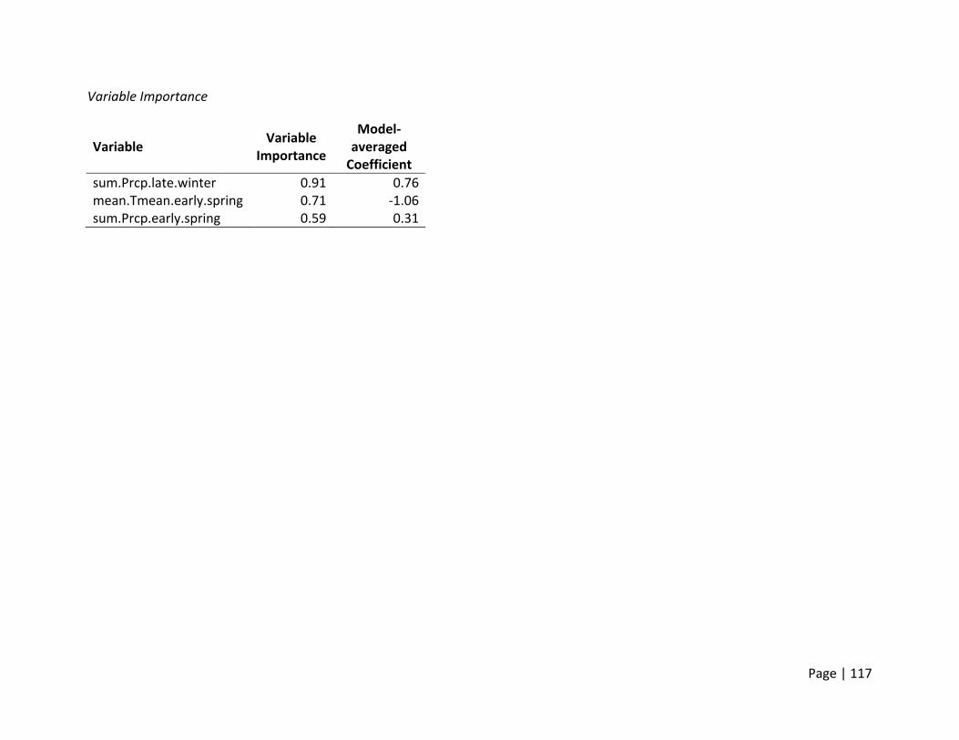
Page | 117

Variable Importance

Variable Variable

Importance


sum.Prcp.late.winter 0.91 0.76mean.Tmean.early.spring 0.71 ‐1.06sum.Prcp.early.spring 0.59 0.31

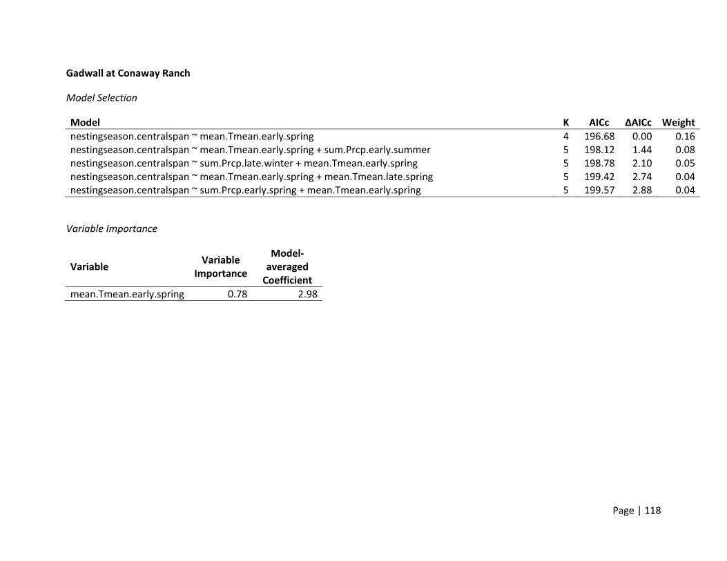
Page | 118


Model Selection


nestingseason.centralspan ~ mean.Tmean.early.spring 4 196.68 0.00 0.16 nestingseason.centralspan ~ mean.Tmean.early.spring + sum.Prcp.early.summer 5 198.12 1.44 0.08 nestingseason.centralspan ~ sum.Prcp.late.winter + mean.Tmean.early.spring 5 198.78 2.10 0.05 nestingseason.centralspan ~ mean.Tmean.early.spring + mean.Tmean.late.spring 5 199.42 2.74 0.04 nestingseason.centralspan ~ sum.Prcp.early.spring + mean.Tmean.early.spring 5 199.57 2.88 0.04

Variable Importance

Variable Variable

Importance


mean.Tmean.early.spring 0.78 2.98

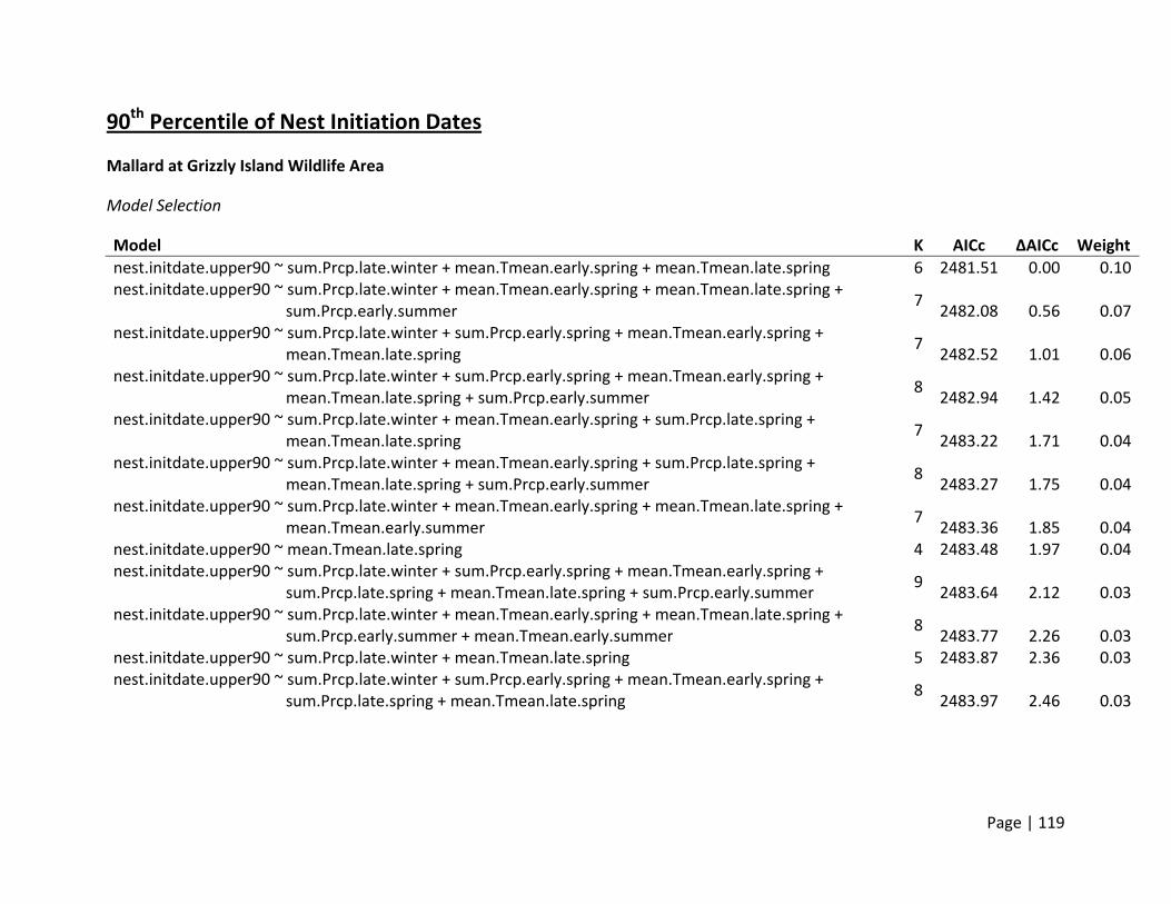
Page | 119

90th Percentile of Nest Initiation Dates


Model Selection


nest.initdate.upper90 ~ sum.Prcp.late.winter + mean.Tmean.early.spring + mean.Tmean.late.spring 6 2481.51 0.00 0.10 nest.initdate.upper90 ~ sum.Prcp.late.winter + mean.Tmean.early.spring + mean.Tmean.late.spring + sum.Prcp.early.summer

7 2482.08 0.56 0.07

nest.initdate.upper90 ~ sum.Prcp.late.winter + sum.Prcp.early.spring + mean.Tmean.early.spring + mean.Tmean.late.spring

7 2482.52 1.01 0.06

nest.initdate.upper90 ~ sum.Prcp.late.winter + sum.Prcp.early.spring + mean.Tmean.early.spring + mean.Tmean.late.spring + sum.Prcp.early.summer

8 2482.94 1.42 0.05

nest.initdate.upper90 ~ sum.Prcp.late.winter + mean.Tmean.early.spring + sum.Prcp.late.spring + mean.Tmean.late.spring

7 2483.22 1.71 0.04

nest.initdate.upper90 ~ sum.Prcp.late.winter + mean.Tmean.early.spring + sum.Prcp.late.spring + mean.Tmean.late.spring + sum.Prcp.early.summer

8 2483.27 1.75 0.04

nest.initdate.upper90 ~ sum.Prcp.late.winter + mean.Tmean.early.spring + mean.Tmean.late.spring + mean.Tmean.early.summer

7 2483.36 1.85 0.04

nest.initdate.upper90 ~ mean.Tmean.late.spring 4 2483.48 1.97 0.04 nest.initdate.upper90 ~ sum.Prcp.late.winter + sum.Prcp.early.spring + mean.Tmean.early.spring + sum.Prcp.late.spring + mean.Tmean.late.spring + sum.Prcp.early.summer

9 2483.64 2.12 0.03

nest.initdate.upper90 ~ sum.Prcp.late.winter + mean.Tmean.early.spring + mean.Tmean.late.spring + sum.Prcp.early.summer + mean.Tmean.early.summer

8 2483.77 2.26 0.03

nest.initdate.upper90 ~ sum.Prcp.late.winter + mean.Tmean.late.spring 5 2483.87 2.36 0.03 nest.initdate.upper90 ~ sum.Prcp.late.winter + sum.Prcp.early.spring + mean.Tmean.early.spring + sum.Prcp.late.spring + mean.Tmean.late.spring

8 2483.97 2.46 0.03

Page | 120

nest.initdate.upper90 ~ sum.Prcp.late.winter + mean.Tmean.late.spring + sum.Prcp.early.summer 6 2484.43 2.92 0.02 nest.initdate.upper90 ~ mean.Tmean.early.spring + mean.Tmean.late.spring 5 2484.50 2.99 0.02

Variable Importance

Variable Variable

Importance


mean.Tmean.late.spring 0.94 ‐1.71sum.Prcp.late.winter 0.79 0.60mean.Tmean.early.spring 0.72 ‐1.37

Page | 121


Model Selection


nest.initdate.upper90 ~ sum.Prcp.late.spring + mean.Tmean.early.summer 5 277.51 0.00 0.19 nest.initdate.upper90 ~ sum.Prcp.late.spring + mean.Tmean.late.spring + mean.Tmean.early.summer 6 279.61 2.10 0.07 nest.initdate.upper90 ~ sum.Prcp.late.winter + sum.Prcp.late.spring + mean.Tmean.early.summer 6 279.65 2.14 0.07 nest.initdate.upper90 ~ sum.Prcp.early.spring + sum.Prcp.late.spring + mean.Tmean.early.summer 6 280.01 2.50 0.05 nest.initdate.upper90 ~ mean.Tmean.early.spring + sum.Prcp.late.spring + mean.Tmean.early.summer 6 280.14 2.63 0.05 nest.initdate.upper90 ~ sum.Prcp.late.spring + sum.Prcp.early.summer + mean.Tmean.early.summer 6 280.18 2.67 0.05

Variable Importance

Variable Variable

Importance


sum.Prcp.late.spring 0.79 2.08mean.Tmean.early.summer 0.78 ‐1.70

Page | 122


Model Selection


nest.initdate.upper90 ~ sum.Prcp.late.winter + sum.Prcp.early.spring + mean.Tmean.early.spring 6 2384.41 0.00 0.06 nest.initdate.upper90 ~ sum.Prcp.late.winter + mean.Tmean.early.spring + sum.Prcp.early.summer + mean.Tmean.early.summer

7 2384.55 0.14 0.06

nest.initdate.upper90 ~ sum.Prcp.late.winter + mean.Tmean.early.spring + mean.Tmean.early.summer 6 2384.63 0.22 0.06 nest.initdate.upper90 ~ sum.Prcp.late.winter + sum.Prcp.early.spring + mean.Tmean.early.spring + sum.Prcp.early.summer

7 2384.67 0.26 0.05

nest.initdate.upper90 ~ sum.Prcp.late.winter + mean.Tmean.early.spring 5 2385.31 0.90 0.04 nest.initdate.upper90 ~ sum.Prcp.late.winter + sum.Prcp.early.spring + mean.Tmean.early.spring + sum.Prcp.early.summer + mean.Tmean.early.summer

8 2385.67 1.26 0.03

nest.initdate.upper90 ~ sum.Prcp.late.winter + sum.Prcp.early.spring + mean.Tmean.early.spring + mean.Tmean.early.summer

7 2385.71 1.31 0.03

nest.initdate.upper90 ~ sum.Prcp.late.winter + mean.Tmean.early.spring + sum.Prcp.early.summer 6 2385.85 1.44 0.03 nest.initdate.upper90 ~ sum.Prcp.late.winter + mean.Tmean.early.spring + mean.Tmean.late.spring 6 2385.90 1.50 0.03 nest.initdate.upper90 ~ sum.Prcp.late.winter + sum.Prcp.early.spring + mean.Tmean.early.spring + mean.Tmean.late.spring

7 2386.06 1.65 0.03

nest.initdate.upper90 ~ sum.Prcp.late.winter + mean.Tmean.early.spring + mean.Tmean.late.spring + mean.Tmean.early.summer

7 2386.23 1.83 0.03

nest.initdate.upper90 ~ sum.Prcp.late.winter + mean.Tmean.early.spring + mean.Tmean.late.spring + sum.Prcp.early.summer + mean.Tmean.early.summer

8 2386.28 1.87 0.02

nest.initdate.upper90 ~ sum.Prcp.late.winter + sum.Prcp.early.spring + mean.Tmean.early.spring + mean.Tmean.late.spring + sum.Prcp.early.summer

8 2386.39 1.98 0.02

nest.initdate.upper90 ~ sum.Prcp.late.winter + mean.Tmean.late.spring 5 2386.45 2.04 0.02 nest.initdate.upper90 ~ sum.Prcp.late.winter + sum.Prcp.early.spring + mean.Tmean.early.spring + 7 2386.45 2.04 0.02

Page | 123

sum.Prcp.late.spring nest.initdate.upper90 ~ sum.Prcp.late.winter + mean.Tmean.early.spring + mean.Tmean.late.spring + sum.Prcp.early.summer

7 2386.48 2.07 0.02

nest.initdate.upper90 ~ sum.Prcp.late.winter + mean.Tmean.early.spring + sum.Prcp.late.spring + mean.Tmean.early.summer

7 2386.53 2.12 0.02

nest.initdate.upper90 ~ sum.Prcp.late.winter + mean.Tmean.early.spring + sum.Prcp.late.spring + sum.Prcp.early.summer + mean.Tmean.early.summer

8 2386.64 2.23 0.02

nest.initdate.upper90 ~ sum.Prcp.late.winter + sum.Prcp.early.spring + mean.Tmean.early.spring + sum.Prcp.late.spring + sum.Prcp.early.summer

8 2386.77 2.36 0.02

nest.initdate.upper90 ~ sum.Prcp.late.winter + mean.Tmean.early.spring + sum.Prcp.late.spring 6 2386.85 2.44 0.02 nest.initdate.upper90 ~ sum.Prcp.late.winter + mean.Tmean.late.spring + sum.Prcp.early.summer 6 2387.04 2.63 0.02

Variable Importance

Variable Variable

Importance


sum.Prcp.late.winter 0.95 1.19mean.Tmean.early.spring 0.76 ‐1.70

Page | 124


Model Selection


nest.initdate.upper90 ~ 1 3 196.22 0.00 0.20 nest.initdate.upper90 ~ sum.Prcp.early.spring 4 198.28 2.06 0.07 nest.initdate.upper90 ~ mean.Tmean.early.spring 4 198.54 2.32 0.06 nest.initdate.upper90 ~ mean.Tmean.early.summer 4 198.64 2.42 0.06 nest.initdate.upper90 ~ mean.Tmean.late.spring 4 198.73 2.51 0.06 nest.initdate.upper90 ~ sum.Prcp.early.summer 4 198.79 2.57 0.05 nest.initdate.upper90 ~ sum.Prcp.late.winter 4 198.95 2.73 0.05 nest.initdate.upper90 ~ sum.Prcp.late.spring 4 199.06 2.84 0.05

Variable Importance


Page | 125



Model Selection


propeggshatched ~ count.extreme.high.95.Tmax + mean.Tmean.late.spring 5 9507.18 0.00 0.11 propeggshatched ~ count.extreme.high.95.Tmax + max.Tmax.late.spring 5 9508.61 1.43 0.06 propeggshatched ~ count.extreme.high.95.Tmax 4 9508.67 1.48 0.05 propeggshatched ~ count.extreme.high.95.Tmax + mean.Tmean.late.spring + max.Tmax.early.summer 6 9509.00 1.82 0.05 propeggshatched ~ count.extreme.high.95.Tmax + mean.Tmean.late.spring + sum.Prcp.early.summer 6 9509.03 1.85 0.04 propeggshatched ~ count.extreme.high.95.Tmax + mean.Tmean.late.spring + max.Tmax.late.spring 6 9509.09 1.91 0.04 propeggshatched ~ count.extreme.high.95.Tmax + sum.Prcp.late.spring + mean.Tmean.late.spring 6 9509.11 1.93 0.04 propeggshatched ~ count.extreme.high.95.Tmax + mean.Tmean.late.spring + mean.Tmean.early.summer 6 9509.13 1.95 0.04 propeggshatched ~ count.extreme.high.95.Tmax + sum.Prcp.late.spring 5 9510.11 2.93 0.03

Variable Importance

Variable Variable

Importance


count.extreme.high.95.Tmax 1.00 ‐0.15mean.Tmean.late.spring 0.59 0.04

Page | 126


Model Selection


propeggshatched ~ count.extreme.high.95.Tmax + sum.Prcp.late.spring + max.Tmax.late.spring + sum.Prcp.early.summer + mean.Tmean.early.summer 8 1261.49 0.00 0.19 propeggshatched ~ count.extreme.high.95.Tmax + sum.Prcp.late.spring + max.Tmax.late.spring + mean.Tmean.early.summer 7 1263.19 1.70 0.08 propeggshatched ~ count.extreme.high.95.Tmax + sum.Prcp.late.spring + max.Tmax.late.spring + sum.Prcp.early.summer + mean.Tmean.early.summer + max.Tmax.early.summer 9 1263.50 2.00 0.07 propeggshatched ~ count.extreme.high.95.Tmax + sum.Prcp.late.spring + mean.Tmean.late.spring + max.Tmax.late.spring + sum.Prcp.early.summer + mean.Tmean.early.summer 9 1263.50 2.01 0.07

Variable Importance

Variable Variable

Importance


count.extreme.high.95.Tmax 0.99 ‐0.12mean.Tmean.early.summer 0.77 ‐0.48sum.Prcp.late.spring 0.72 0.40max.Tmax.late.spring 0.64 0.19sum.Prcp.early.summer 0.53 0.45

Page | 127


Model Selection


propeggshatched ~ count.extreme.high.95.Tmax + mean.Tmean.late.spring + mean.Tmean.early.summer 6 2337.34 0.00 0.09 propeggshatched ~ count.extreme.high.95.Tmax + max.Tmax.late.spring + mean.Tmean.early.summer 6 2338.23 0.89 0.06 propeggshatched ~ count.extreme.high.95.Tmax + mean.Tmean.late.spring + max.Tmax.late.spring + mean.Tmean.early.summer

7 2338.48 1.14 0.05

propeggshatched ~ count.extreme.high.95.Tmax + mean.Tmean.late.spring + sum.Prcp.early.summer + mean.Tmean.early.summer

7 2338.80 1.45 0.04

propeggshatched ~ count.extreme.high.95.Tmax + mean.Tmean.late.spring + mean.Tmean.early.summer + max.Tmax.early.summer

7 2338.83 1.49 0.04

propeggshatched ~ count.extreme.high.95.Tmax + sum.Prcp.late.spring + mean.Tmean.late.spring + mean.Tmean.early.summer

7 2339.26 1.92 0.03

propeggshatched ~ max.Tmax.late.spring + mean.Tmean.early.summer 5 2339.32 1.97 0.03 propeggshatched ~ count.extreme.high.95.Tmax + sum.Prcp.late.spring + max.Tmax.late.spring + mean.Tmean.early.summer

7 2339.67 2.32 0.03

propeggshatched ~ count.extreme.high.95.Tmax + mean.Tmean.late.spring + sum.Prcp.early.summer + mean.Tmean.early.summer + max.Tmax.early.summer

8 2339.94 2.60 0.02

propeggshatched ~ count.extreme.high.95.Tmax + max.Tmax.late.spring + sum.Prcp.early.summer + mean.Tmean.early.summer

7 2340.07 2.73 0.02

propeggshatched ~ count.extreme.high.95.Tmax + mean.Tmean.late.spring + max.Tmax.late.spring + sum.Prcp.early.summer + mean.Tmean.early.summer

8 2340.10 2.75 0.02

propeggshatched ~ mean.Tmean.late.spring + max.Tmax.late.spring + mean.Tmean.early.summer 6 2340.22 2.88 0.02 propeggshatched ~ count.extreme.high.95.Tmax + max.Tmax.late.spring + mean.Tmean.early.summer + max.Tmax.early.summer

7 2340.23 2.89 0.02

Page | 128

Variable Importance

Variable Variable

Importance


mean.Tmean.early.summer 0.84 0.14count.extreme.high.95.Tmax 0.77 ‐0.08mean.Tmean.late.spring 0.59 ‐0.05max.Tmax.late.spring 0.55 ‐0.02

Page | 129


Model Selection


propeggshatched ~ sum.Prcp.late.spring + mean.Tmean.early.summer 5 262.48 0.00 0.08 propeggshatched ~ count.extreme.high.95.Tmax + sum.Prcp.late.spring + mean.Tmean.early.summer 6 263.94 1.46 0.04 propeggshatched ~ max.Tmax.late.spring 4 264.20 1.71 0.03 propeggshatched ~ mean.Tmean.late.spring 4 264.36 1.88 0.03 propeggshatched ~ sum.Prcp.late.spring + sum.Prcp.early.summer + mean.Tmean.early.summer 6 264.41 1.93 0.03 propeggshatched ~ mean.Tmean.late.spring + mean.Tmean.early.summer 5 264.42 1.93 0.03 propeggshatched ~ mean.Tmean.late.spring + max.Tmax.early.summer 5 264.48 1.99 0.03 propeggshatched ~ mean.Tmean.early.summer 4 264.55 2.07 0.03 propeggshatched ~ sum.Prcp.late.spring + max.Tmax.late.spring + mean.Tmean.early.summer 6 264.70 2.22 0.03 propeggshatched ~ sum.Prcp.late.spring + mean.Tmean.late.spring + mean.Tmean.early.summer 6 264.82 2.33 0.03 propeggshatched ~ sum.Prcp.late.spring + mean.Tmean.early.summer + max.Tmax.early.summer 6 264.82 2.33 0.03 propeggshatched ~ max.Tmax.late.spring + mean.Tmean.early.summer 5 265.24 2.76 0.02 propeggshatched ~ count.extreme.high.95.Tmax + mean.Tmean.late.spring + mean.Tmean.early.summer 6 265.25 2.77 0.02 propeggshatched ~ count.extreme.high.95.Tmax + max.Tmax.late.spring 5 265.43 2.95 0.02

Variable Importance

Variable Variable

Importance


mean.Tmean.early.summer 0.65 ‐0.35

Page | 130

Nest Survival


Model Selection

BASE MODEL = date.julian + nestage + adj.initdate + date.julian:adj.initdate + nestage:adj.initdate


count.extreme.high.95.Tmax + mean.Tmean + sum.Prcp + sum.Prcp.early.spring + sum.Prcp.late.spring 11 21720.42 0.00 1.00

Variable Importance

Variable Variable

Importance

Model‐averaged Coefficient*

count.extreme.high.95.Tmax 1.00 0.38mean.Tmean 1.00 ‐0.07sum.Prcp 1.00 0.68sum.Prcp.early.spring 1.00 0.03sum.Prcp.late.spring 1.00 ‐0.05

*NOTE: Model averaged coefficients for nest‐survival model are with respect to the logit transformation in model.

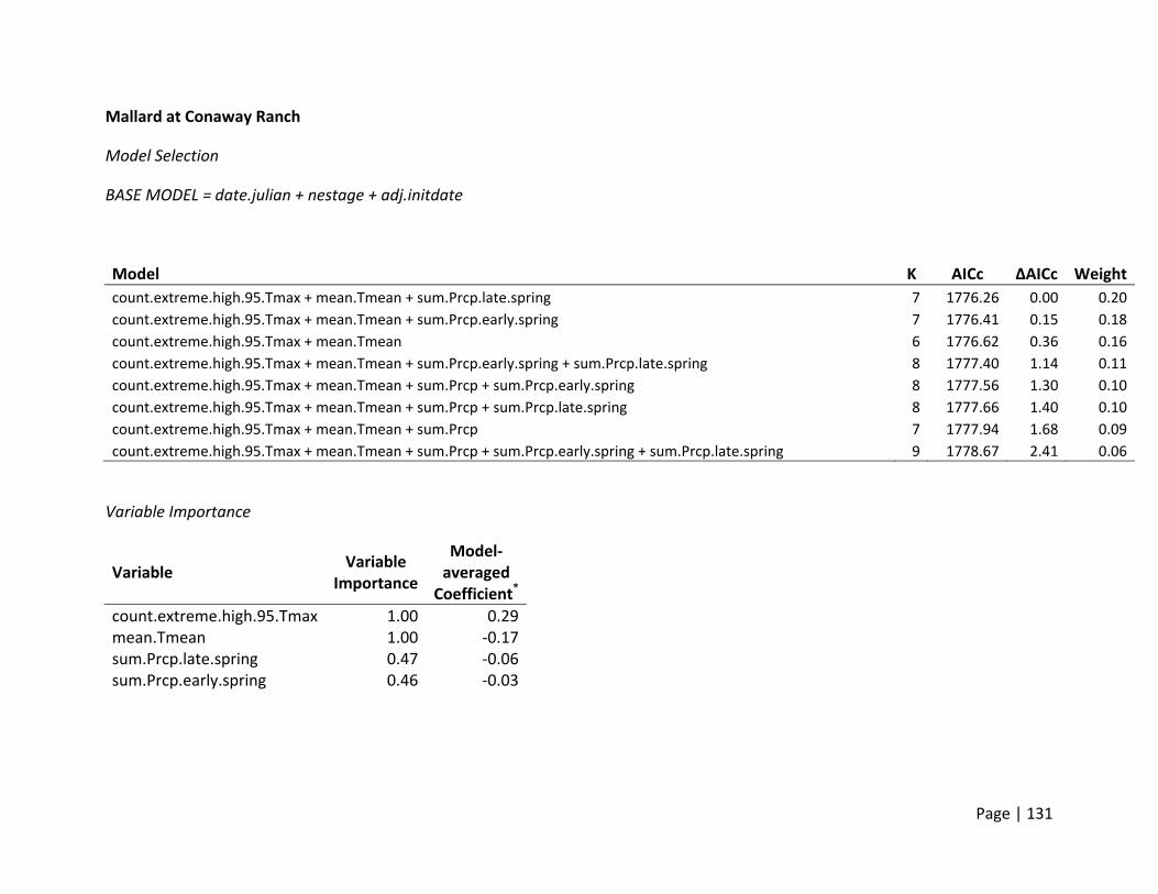
Page | 131


Model Selection

BASE MODEL = date.julian + nestage + adj.initdate


count.extreme.high.95.Tmax + mean.Tmean + sum.Prcp.late.spring 7 1776.26 0.00 0.20

count.extreme.high.95.Tmax + mean.Tmean + sum.Prcp.early.spring 7 1776.41 0.15 0.18

count.extreme.high.95.Tmax + mean.Tmean 6 1776.62 0.36 0.16

count.extreme.high.95.Tmax + mean.Tmean + sum.Prcp.early.spring + sum.Prcp.late.spring 8 1777.40 1.14 0.11

count.extreme.high.95.Tmax + mean.Tmean + sum.Prcp + sum.Prcp.early.spring 8 1777.56 1.30 0.10

count.extreme.high.95.Tmax + mean.Tmean + sum.Prcp + sum.Prcp.late.spring 8 1777.66 1.40 0.10

count.extreme.high.95.Tmax + mean.Tmean + sum.Prcp 7 1777.94 1.68 0.09


Variable Importance

Variable Variable

Importance


count.extreme.high.95.Tmax 1.00 0.29mean.Tmean 1.00 ‐0.17sum.Prcp.late.spring 0.47 ‐0.06sum.Prcp.early.spring 0.46 ‐0.03

Page | 132

sum.Prcp 0.34 ‐0.22*NOTE: Model averaged coefficients for nest‐survival model are with respect to the logit transformation in model.


Model Selection

BASE MODEL = nestage + adj.initdate + nestage^2 + adj.initdate^2


count.extreme.high.95.Tmax + mean.Tmean + sum.Prcp 8 6183.20 0.00 0.23


count.extreme.high.95.Tmax + mean.Tmean + sum.Prcp + sum.Prcp.late.spring 9 6183.38 0.18 0.21



Variable Importance

Variable Variable

Importance


count.extreme.high.95.Tmax 1.00 0.42mean.Tmean 1.00 ‐0.10sum.Prcp 0.82 0.27sum.Prcp.late.spring 0.55 0.03Sum.Prcp.early.spring 0.48 ‐0.01

*NOTE: Model averaged coefficients for nest‐survival model are with respect to the logit transformation in model.

Page | 133


Model Selection

BASE MODEL = nestage + adj.initdate


count.extreme.high.95.Tmax + mean.Tmean + sum.Prcp.early.spring 6 282.39 0.00 0.33


count.extreme.high.95.Tmax + mean.Tmean 5 284.30 1.91 0.13


count.extreme.high.95.Tmax + mean.Tmean + sum.Prcp.late.spring 6 284.81 2.42 0.10

Variable Importance

*NOTE: Model averaged coefficients for nest‐survival model are with respect to the logit transformation in model

Variable Variable

Importance


count.extreme.high.95.Tmax 0.95 0.27mean.Tmean 0.95 ‐0.22sum.Prcp.early.spring 0.63 ‐0.09sum.Prcp.late.spring 0.31 0.06sum.Prcp 0.29 0.48

Documents

A Multi‐Sp and Multi‐LLands App - CA Climate Commonsclimate.calcommons.org/sites/default/files/Avian... · 2014-11-03 · 1 65 68 71 73 76 Grizzly Island--Mallard Number of Days