A Multi-temporal Analysis of AMSR-E Data for Flood and

City University of New York (CUNY) City University of New York (CUNY)

CUNY Academic Works CUNY Academic Works

Publications and Research City College of New York

2011

A Multi-temporal Analysis of AMSR-E Data for Flood and A Multi-temporal Analysis of AMSR-E Data for Flood and

Discharge Monitoring during the 2008 Flood in Iowa Discharge Monitoring during the 2008 Flood in Iowa

Marouane Temimi CUNY City College

Teodosio Lacava National Research Council

Tarendra Lakhankar CUNY City College

Valerio Tramutoli University of Basilicata

Hosni Ghedira Masdar Institute

See next page for additional authors

How does access to this work benefit you? Let us know!

More information about this work at: https://academicworks.cuny.edu/cc_pubs/220

Discover additional works at: https://academicworks.cuny.edu

This work is made publicly available by the City University of New York (CUNY). Contact: [email protected]

https://academicworks.cuny.edu/

https://academicworks.cuny.edu/cc_pubs

https://academicworks.cuny.edu/cc

http://ols.cuny.edu/academicworks/?ref=https://academicworks.cuny.edu/cc_pubs/220

https://academicworks.cuny.edu/cc_pubs/220

https://academicworks.cuny.edu/?

mailto:[email protected]

Authors Authors Marouane Temimi, Teodosio Lacava, Tarendra Lakhankar, Valerio Tramutoli, Hosni Ghedira, Riadh Ata, and Reza Khanbilvardi

This article is available at CUNY Academic Works: https://academicworks.cuny.edu/cc_pubs/220

https://academicworks.cuny.edu/cc_pubs/220

HYDROLOGICAL PROCESSESHydrol. Process. 25, 2623–2634 (2011)Published online 4 March 2011 in Wiley Online Library(wileyonlinelibrary.com) DOI: 10.1002/hyp.8020

A multi-temporal analysis of AMSR-E data for floodand discharge monitoring during the 2008 flood in Iowa

Marouane Temimi,1* Teodosio Lacava,2 Tarendra Lakhankar,1 Valerio Tramutoli,3

Hosni Ghedira,4 Riadh Ata5 and Reza Khanbilvardi1

1 NOAA-CREST, City University of New York, 160 Convent Avenue, New York, NY, 10031, USA2 Institute of Methodologies for Environmental Analysis (IMAA) –National Research Council (CNR), C.da Santa Loja, 85050, Tito Scalo (PZ), Italy

3 Department of Engineering and Physics of Environment (DIFA) –University of Basilicata –via dell’Ateneo Lucano, 10, 85100 Potenza, Italy4 Water and Environmental Engineering Program, Masdar Institute, Abu Dhabi, United Arab Emirates

5 Electricite de France EDF LNHE/ National Hydraulics and Environment Lab., Chatou, France

Abstract:

The objective of this work is to demonstrate the potential of using passive microwave data to monitor flood and dischargeconditions and to infer watershed hydraulic and hydrologic parameters. The case study is the major flood in Iowa in summer2008. A new Polarisation Ratio Variation Index (PRVI) was developed based on a multi-temporal analysis of 37 GHz satelliteimagery from the Advanced Microwave Scanning Radiometer (AMSR-E) to calculate and detect anomalies in soil moistureand/or inundated areas. The Robust Satellite Technique (RST) which is a change detection approach based on the analysis ofhistorical satellite records was adopted. A rating curve has been developed to assess the relationship between PRVI valuesand discharge observations downstream. A time-lag term has been introduced and adjusted to account for the changing delaybetween PRVI and streamflow. Moreover, the Kalman filter has been used to update the rating curve parameters in near realtime. The temporal variability of the b exponent in the rating curve formula shows that it converges toward a constant value.A consistent 21-day time lag, very close to an estimate of the time of concentration, was obtained. The agreement betweenobserved discharge downstream and estimated discharge with and without parameters adjustment was 65 and 95%, respectively.This demonstrates the interesting role that passive microwave can play in monitoring flooding and wetness conditions andestimating key hydrologic parameters. Copyright 2011 John Wiley & Sons, Ltd.

KEY WORDS flood; river discharge; soil moisture; passive microwave; Kalman filter

Received 9 April 2010; Accepted 20 January 2011

INTRODUCTION

Major floods were observed in Upper Mississippi Water-shed in June 2008. Much of central and eastern Iowawas affected by a 500-year flood which was classifiedas the worst in the history of the region (http://www.flood2008.iowa.gov/). Major damages and large inun-dated areas related to these floods have been recorded.Remote sensing data and particularly, passive microwaveimages, have been largely used to monitor these extremeevents (Crow et al., 2005; Schmugge, 1998; Sippel et al.,1998). Three main reasons motivate the use of passivemicrowave data which are namely their high temporalresolution, their large spatial coverage and the capabil-ity of the signal to penetrate through clouds. Despite thegreat interest in low frequencies such as L and C bandswhich are more appropriate for soil moisture retrieval,other studies have explored the potential of the 37 GHzchannel to monitor flood conditions (Brakenridge et al.,2007; Sippel et al., 1994; Tanaka et al., 2000; Ferrazzoliet al. 2010).

* Correspondence to: Marouane Temimi, NOAA-CREST, City Universityof New York, 160 Convent Avenue, New York, NY, 10031, USA.E-mail: [email protected]

The 37-GHz Polarisation Difference (PD D Tbv �Tbh) where Tb is the brightness temperature and v/hrefers to vertical/horizontal polarisation has been used tomonitor flooded areas (Choudhury, 1989; Sippel et al.,1994; Tanaka et al., 2003). Sippel et al. (1994) appliedthe index to delineate the extent of flooding along theAmazon River through the use of an established rela-tionship between the river stage and flooded area extent(Sippel et al., 1998). A similar relationship was also suc-cessfully applied by Hamilton et al. (2004). Kerr andNjoku (1993) used, on the other hand, the Polarisa-tion Ratio (PR D �Tbv � Tbh�/�Tbv C Tbh�) because itis less affected by atmospheric conditions and insensi-tive to surface temperature (Njoku and Chan, 2006; Oweet al., 2001). The same index was used by Paloscia et al.(2001) to assess the vegetation effect and to retrievesoil moisture using observations from the Special SensorMicrowave Imager (SSM/I). In order to distinguish thesoil moisture contribution from vegetation and soil rough-ness contributions to the measured signal, Lacava et al.(2005a) successfully applied the Robust Satellite Tech-niques (RST) approach (Tramutoli et al., 2005, 2007)to Advanced Microwave Sounding Unit (AMSU) data.More recently, Temimi et al. (2007) used PR with otherancillary data to account for vegetation heterogeneity and

Copyright 2011 John Wiley & Sons, Ltd.

2624 M. TEMIMI ET AL.

to estimate soil moisture in a large northern watershed.Also, Tanaka et al. (2003) have found a good agreementbetween derived water extent from brightness tempera-ture observed at 37 GHz and AVHRR images.

The use of microwave observations at high frequen-cies was also expanded to infer hydraulic variables.Brakenridge et al. (2007) used AMSR-E 37 GHz bright-ness temperature to globally infer river discharge. Thesame AMSR-E frequency was also used by Temimiet al. (2005) to monitor streamflow in the MackenzieRiver Basin in Canada. Their findings coincided withthose by Smith et al. (1996) and Bjerklie et al. (2003)which demonstrated the feasibility of measuring riverdischarge from space. In another study, Smith and Pavel-sky (2008) estimated the flood wave propagation speedusing remote sensing data. Their analysis was basedon a rating curve relationship which is largely used inriver hydraulics to estimate river discharge or stage (Fra-zier et al., 2003; Smith et al., 1996). The river effectivewidth has been used as proxy for the inundation extent(Ashmore and Sauks, 2006; Smith and Pavelsky, 2008).Smith and Pavelsky (2008) also demonstrated the pos-sible transferability of this relationship between differ-ent sections along the river. In addition, Bjerklie et al.(2003, 2005) have inferred river discharge using remotelysensed hydraulic variables. Other studies demonstratedthat assimilating satellite based discharge estimates intohydrological/hydraulic models lead to an improvementin their performance (Montanari et al., 2009; Neal et al.,2009).

This study investigates the use of passive microwavedata for flood and river discharge monitoring. In particu-lar, the relationship between the extent of inundated/wetareas and observed discharge downstream is analysed.Also, the potential of using passive microwave data toassess key hydrologic and hydraulic parameters is eval-uated.

METHODOLOGY

Study area

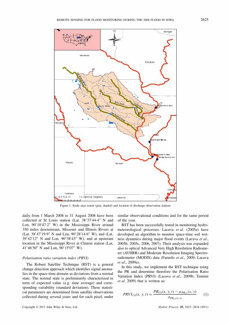
The study area which was largely affected by theflood event in 2008 is located in Iowa and part of theUpper Mississippi watershed (Figure 1). It is drainedby the Des Moines, Cedar, and Iowa Rivers whichare tributaries of the Mississippi River. During the firstweek of June 2008, very intense precipitations havebeen recorded throughout the Midwest and particularlyin Iowa. Most of these precipitations occurred over ashort period of time and generated flash flood conditions.It is very important to add that these rainfalls werepreceded by a particularly wet winter and spring seasons.These exceptional conditions were the second wettestsince 1895 (NCDC, 2008). They fostered the drainageof almost the total amount of rainfall received in June.

The Turkey River, the Maquoketa River, the UpperIowa River, the Iowa River (and its main tributaries),the Cedar River (and its main tributaries), and the Skunk

River all exceeded their overbank flooding stages. Theflood burst at least 25 levees in Missouri, Iowa, andIllinois. Two of the largest cities in Iowa, Iowa Cityof Johnson County and Cedar Rapids of Linn Countywere significantly affected by the flooding (Hoke, 2009).Cedar River inundated a large portion of Cedar Rapidswith 12 foot flood-stage causing substantial damages of avalue around US $737 million (Coleman and Budikova,2010). The total cost of the damages associated to theflood event is around US $10 billion. By mid-June, theFederal Emergency Management Agency (FEMA) haddeclared 85 out of the 99 Iowa counties disaster areas.An estimation of 1Ð2 million acres of corn and soybeancrops was lost due to the flood (RIO, 2009).

Areas along the Iowa River and its major tributary,Cedar River, were the most affected by the 2008 floodevent. Des Moines River, the second largest River inthe state after Iowa River, was also subject to overbankflooding. Three main reservoirs exist along these rivers.The impact of these reservoirs on the drainage delayand its relationship with the discharge downstream in theMississippi river is not considered in this study.

Data

The proposed methodology makes use of AMSR-Evertically and horizontally polarized brightness temper-atures observed at 37 GHz from June 2002 to August2008. AMSR-E observations are taken at least twice aday from ascending and descending overpasses. AMSR-Elevel 2A product has been used in this study. All AMSR-E data were obtained from National Snow and Ice DataCenter (http://nsidc.org).

The Field of View (FOV) of AMSR-E is larger atlower frequencies as it varies from 43 ð 75 km at the6Ð9 GHz to 8 ð 14 km at the 37 GHz channel. The37 GHz channel compromises between spatial resolutionand atmospheric perturbations. AMSR-E observations atlower frequencies (i.e. 6Ð7, 10Ð7, and 19 GHz), despitetheir sensitivity to soil moisture, are relatively coarsein term of spatial resolution. The 89 GHz channel hasthe finest spatial resolution (5 km). However, it is sub-stantially affected by atmospheric perturbations mainlybecause of the O2 contamination (Brakenridge et al.,2007). Recently, Ferrazzoli et al. (2010) have monitoredrainstorm and flooding events through the estimationof the polarisation ratio at three AMSR-E frequenciesnamely, the 6Ð9, 10Ð7, and 37 GHz which correspond tothe C, X, and Ka bands respectively. They noticed bettercapabilities in delineating the waterbodies and inundatedareas at the Ka band because of the higher spatial res-olution. In term of temporal variation the polarisationratios at the three frequencies have shown very similarbehaviour with a mitigated temporal variability at the Cband.

In this study, we are expanding our analysis to thetime periods before and after the flood event to bettercomprehend the drainage delays with respect to the mag-nitude of the flood event and study the link with dis-charge observed downstream. Rivers discharge observed

Copyright 2011 John Wiley & Sons, Ltd. Hydrol. Process. 25, 2623–2634 (2011)

REMOTE SENSING FOR FLOOD MONITORING DURING THE 2008 FLOOD IN IOWA 2625

Figure 1. Study area extent (gray shaded) and location of discharge observation stations

daily from 1 March 2008 to 31 August 2008 have beencollected at St Louis station (Lat. 38°37044Ð400 N andLon. 90°10047Ð200 W) in the Mississippi River around350 miles downstream, Missouri and Illinois Rivers at(Lat. 38°47019Ð900 N and Lon. 90°28014Ð600 W), and (Lat.39°4201200 N and Lon. 90°3804300 W), and at upstreamlocation in the Mississippi River at Clinton station (Lat,41°4605000 N and Lon, 90°1500700 W).

Polarisation ratio variation index (PRVI)

The Robust Satellite Technique (RST) is a generalchange detection approach which identifies signal anoma-lies in the space-time domain as deviations from a normalstate. The normal state is preliminarily characterized interm of expected value (e.g. time average) and corre-sponding variability (standard deviation). These statisti-cal parameters are determined from satellite observationscollected during several years and for each pixel, under

similar observational conditions and for the same periodof the year.

RST has been successfully tested in monitoring hydro-meteorological processes. Lacava et al. (2005a) havedeveloped an algorithm to monitor space-time soil wet-ness dynamics during major flood events (Lacava et al.,2005b, 2005c, 2006, 2007). Their analysis was expandedalso to optical Advanced Very High Resolution Radiome-ter (AVHRR) and Moderate Resolution Imaging Spectro-radiometer (MODIS) data (Faruolo et al., 2009; Lacavaet al., 2009a).

In this study, we implement the RST technique usingthe PR and determine therefore the Polarisation RatioVariation Index (PRVI) (Lacava et al., 2009b; Temimiet al. 2009) that is written as:

PRVICh�x, y, t� D PRCh�x, y, t� � �PRCh�x, y�

�PRCh�x,y��1�



where PRCh�x, y, t� is the PR computed for an AMSR-E channel ‘Ch’ (i.e. 37 GHz in this work); �PRCh�x, y�and �PRCh�x, y� are the time average and standard devi-ation of PRCh�x, y, t� computed, for the pixel centeredat (x,y) coordinates. The time average �PRCh�x, y� andthe standard deviation �PRCh�x, y� are determined frommulti-annual AMSR-E imagery dataset which only con-tains data collected during the same month of the yearand acquired at the same hour of the day. Imagesacquired from 2002 to 2007 were used to determinethe monthly average, �PRCh�x, y� and �PRCh�x, y�, fromMarch through August, on pixel-per-pixel basis. AMSR-E images observed in 2008, from March through August,were used to calculate PRVI Ch�x, y, t�.

The PRVI Ch�x, y, t� gives then, for each pixel (x,y) andtime t of observation, the actual PR excess (comparedto its unperturbed conditions) weighted by its normalvariability, historically assessed under similar observa-tional conditions. Hereafter, we will use PRVI referringto PRVI 37 GHz�x, y, t�. It is expected that the proposedPRVI reduces the impact of site effects (known or not)and mitigates the impact of spurious effects like thoserelated to the presence of Radio Frequency Interference(RFI) at AMSR-E low frequencies (Lacava et al., 2009c).

If we assume that the vegetation cover has a relativeslower temporal variation with respect to soil moistureand that its seasonal variation follows almost the samecycle every year, one should expect that PRVI predomi-nately reflects changes in flooded areas and soil moisturesince �PRCh�x, y� and the standard deviation �PRCh�x, y�are estimated on a monthly basis to account for this sea-sonal variation. It is expected that PRVI increases sharplywhen overbank flooding occurs. PRVI should qualita-tively reflect changes in total surface wetness i.e. soilmoisture and open waterbodies (permanent and flooded).

Although passive microwave data are all-sky capa-ble, atmospheric perturbations introduced by rainy cloudsare inherent particularly at high frequencies such as the37 GHz. It is therefore necessary to account for theseprocesses. Modelling the impact of rainy clouds on thepassive microwave signal is complex and not straight-forward. Thus, in this study, heavy rainfall conditionswere detected and masked using a threshold-based tech-nique which utilizes observed brightness temperaturesat 89 GHz vertical polarisation. According to Grody(1991), a work on SSM/I (Special Sensor MicrowaveImager) data which was expanded later by Wilheit et al.(2003) to AMSR-E observations, brightness temperaturesat 89 GHz vertical polarisation less than 210 K may beattributed to intense precipitation. The implementation ofa more sophisticated approach is possible but it is beyondthe scope of this work. Pixels corresponding to heavyrainfall conditions have been eliminated through a com-positing technique which consists in retaining the latestPRVI value corresponding to non-rainy conditions overevery pixel showing intense precipitation.

Adjustment of the rating curve parameters

Considering the sensitivity of PRVI to change inwetness and flooding conditions and the impact of thischange on river discharge, we suggest writing the ratingcurve formula as:

Q�t� D a PRVI�t�b �2�

where Q is the estimated discharge downstream and a andb are two empirical parameters. The b parameter whichis also known as the width exponent is an indicator ofriver behaviour and morphology (Smith and Pavelsky,2008). The drainage of inundated areas and/or wet soilsincreases the streamflow downstream. The rating curvemakes use of this causality to establish a relationshipbetween the magnitude of the flood upstream (as sensedby PRVI) and observed discharge downstream.

The rating curve formula in Equation (2) supposes thatPRVI (whether it is caused by flood or soil moisture) anddischarge are in phase. However, a lag has always beenobserved, due to drainage delay, between the maximumof water surface area and the peak of the flow (Bindlishet al., 2009). Therefore, the rating curve formula may bewritten as:

Q�t� D a. PRVIb�t � d.t� if t > d.t �3�

Where, d.t is the delay between discharge down-stream and PRVI. The time lag depends on the precipita-tion spatial distribution and return period. It should alsodepend on antecedent soil moisture conditions, surfaceroughness and vegetation density. So, assuming a con-stant time lag may lead to a disparity between estimatedand observed discharge. Typically, the lag cannot exceedthe time of concentration of the watershed (i.e. drainagetime plus travel time). In the present study, the time lagterm maximizes the value of the cross-correlation func-tion between discharge and PRVI. The cross-correlationfunction is calculated at every time step and the phaselag is regularly updated.

Other factors such as the morphology of the river, itsslope, and roughness can affect the relationship betweenthe observed discharge and the remotely derived wetnessthrough PRVI. There are also dynamic factors suchas the infiltration capacity of the watershed and itsrunoff coefficient as well as the flood wave propagationspeed. The variability of these factors has an impacton the relationship between discharge and PRVI. It istherefore necessary to monitor this impact by updatingthe parameters of the rating curve through the use ofthe Kalman filter. The application of the logarithm toEquation (3) allows writing the rating curve relationshipas:

Log�Q�t�� D log�a� C b log �PRVI�t � d.t�� 4�

or Y D B C A X �5�

where: Y D log (Q�t�)

X D log (PRVI(t � d.t))



0

0.005

0.01

0.015

0.02

0.025

0.03

0.035

0.04

17-Mar

24-Mar

31-Mar

7-Apr

14-Apr

21-Apr

28-Apr

5-May

12-May

19-May

26-May

2-Jun

9-Jun

16-Jun

23-Jun

30-Jun

7-Jul

14-Jul

21-Jul

28-Jul

4-Aug

11-Aug

18-Aug

25-Aug

Date

Po

lari

zati

on

Rat

io (

PR

)

Observed PR Monthly PR mean Standard Deviation

MarchApril

May

June

July August

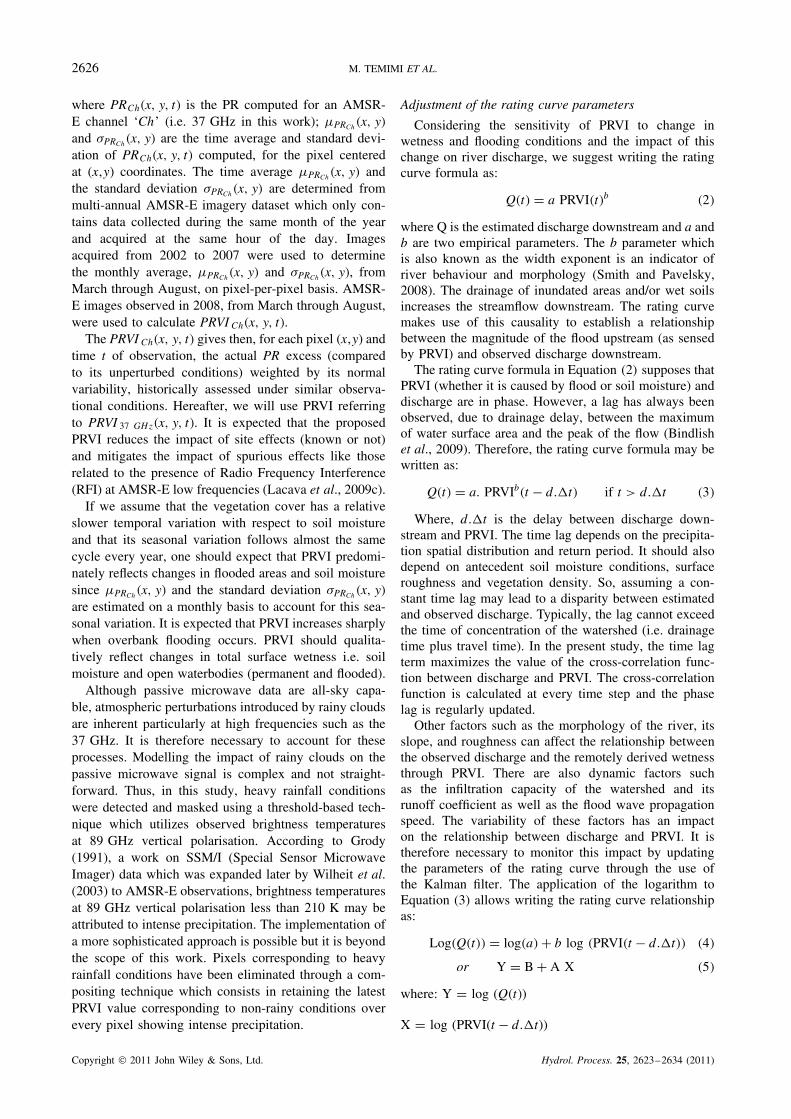
Figure 2. Seasonal variation of the areal average PR in 2008 compared to the mean and standard deviation computed for each month over the entirestudy area

A and B are the two model’s parameters.

The Kalman filter (Johns and Mandel, 2008; Pan andWood, 2006) is applied to the rating curve model byconsidering the state and the observation equations whichare written as:

AtC1 D tAt C Wt �6�

Yt D HtAt C Vt �7�

where, Y subscript D Y

At D[

AB

]

Ht D [ X 1 ]

Y D log (Q�t�) and X D log (PRVI(t � d.t));Wt and Vt are the model and observation noises whichare assumed to be zero mean Gaussian white noises.

The dynamic rating curve model continuously readjustsits parameters to satisfy the non-stationary behaviour ofthe hydrological phenomenon. The rating curve relation-ship is typically site specific (Ashmore and Sauks, 2006;Frazier et al., 2003) and cannot be expanded to otherrivers without a preliminary calibration step. The use ofthe Kalman filter adds an adaptive capability to the rat-ing curve formula and makes it flexible and expandableto different watersheds. However, the expansion of thetechnique should be done with caution as it requires theexistence of a minimum of causality between dischargeand PRVI. A preliminary analysis is always required toverify these conditions.

It is expected that this approach leads through thedevelopment of an adaptive rating curve to a better under-standing of the dynamic of the hydrological processes andthe variability of key hydrologic and hydraulic parame-ters. It is important to note that the ultimate objectiveof this work is not predicting streamflow downstreambut exploring the role that passive microwave can playin monitoring its variability. The adjustment of the ratingcurve parameters leads to an assessment of their change intime and contribute to improve our understanding of theirvariability with respect to watershed and rainfall charac-teristics. This can ultimately lead to the development of arelationship between these variables and the river’s geo-morphologic parameters. Such relationship may allow usto overcome the necessary calibration step in the case ofstandard rating curve and assess the rating curve param-eters at ungauged sites (Smith and Pavelsky, 2008).

RESULTS AND DISCUSSIONS

The areal average PR tends to increase in spring untilreaching a maximum in May and then decreases towardsthe end of the summer. Standard deviation is also thehighest in May indicating significant variations of the PRwhich can be attributed to excessive wetness generationfrom snowmelt, runoff, and precipitation. The analysis ofPR fluctuations covered the time period from March toAugust 2008. Figure 2 shows the intraseasonal variabilityof the observed PR which was spatially averaged overthe study area. Figure 2 also compares PR to monthly



−0.01

−0.005

0

0.005

0.01

0.015

0.02

0.025

0.03

0.035

0.04

3/17/2008 4/17/2008 5/17/2008 6/17/2008 7/17/2008 8/17/2008

Date

PR

an

d P

RV

I/100

0.00

5.00

10.00

15.00

20.00

25.00

30.00

35.00

40.00

45.00

50.00

Pre

cip

itat

ion

(m

m)

Total precipitation Areal average PR Areal average PRVI

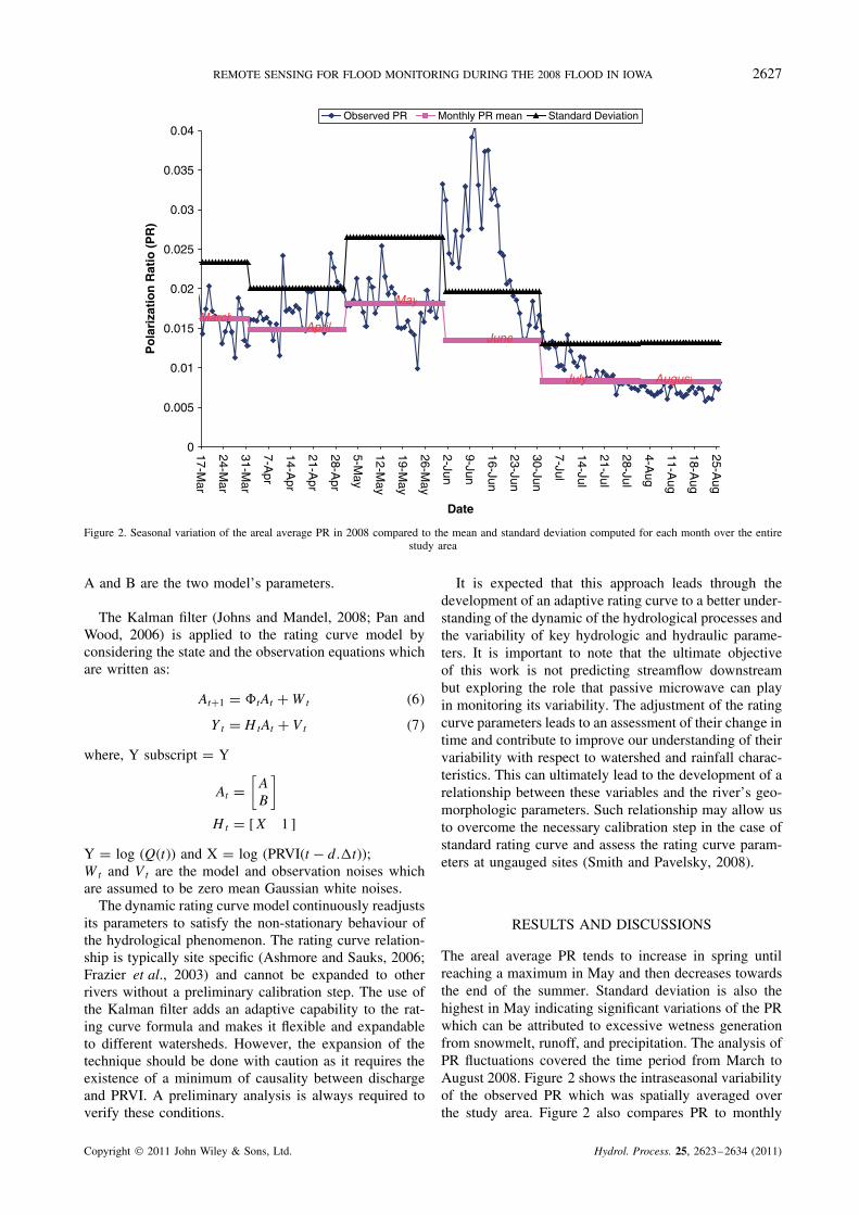
Figure 3. Calculated PR and PRVI compared to total precipitation recorded across the study area

mean and standard deviation computed through theimplementation of the RST approach.

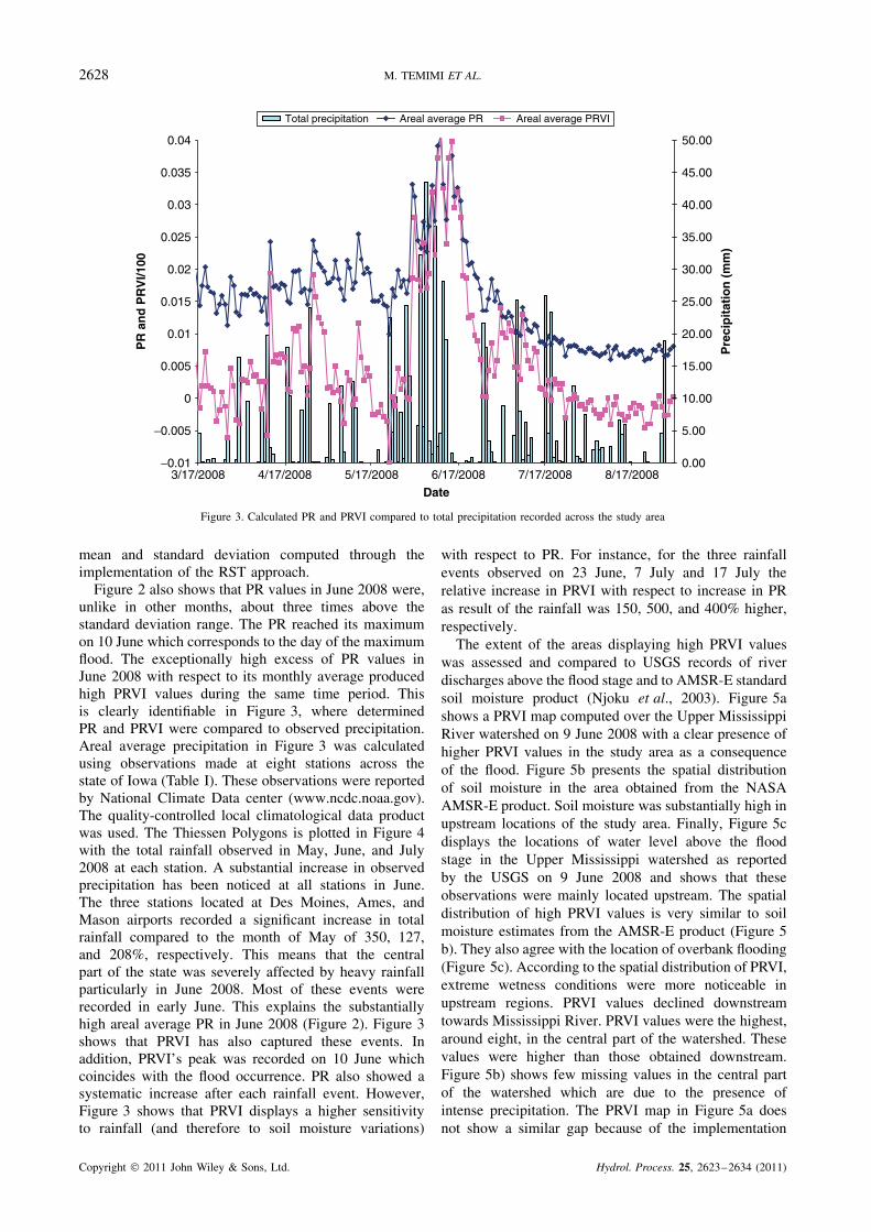
Figure 2 also shows that PR values in June 2008 were,unlike in other months, about three times above thestandard deviation range. The PR reached its maximumon 10 June which corresponds to the day of the maximumflood. The exceptionally high excess of PR values inJune 2008 with respect to its monthly average producedhigh PRVI values during the same time period. Thisis clearly identifiable in Figure 3, where determinedPR and PRVI were compared to observed precipitation.Areal average precipitation in Figure 3 was calculatedusing observations made at eight stations across thestate of Iowa (Table I). These observations were reportedby National Climate Data center (www.ncdc.noaa.gov).The quality-controlled local climatological data productwas used. The Thiessen Polygons is plotted in Figure 4with the total rainfall observed in May, June, and July2008 at each station. A substantial increase in observedprecipitation has been noticed at all stations in June.The three stations located at Des Moines, Ames, andMason airports recorded a significant increase in totalrainfall compared to the month of May of 350, 127,and 208%, respectively. This means that the centralpart of the state was severely affected by heavy rainfallparticularly in June 2008. Most of these events wererecorded in early June. This explains the substantiallyhigh areal average PR in June 2008 (Figure 2). Figure 3shows that PRVI has also captured these events. Inaddition, PRVI’s peak was recorded on 10 June whichcoincides with the flood occurrence. PR also showed asystematic increase after each rainfall event. However,Figure 3 shows that PRVI displays a higher sensitivityto rainfall (and therefore to soil moisture variations)

with respect to PR. For instance, for the three rainfallevents observed on 23 June, 7 July and 17 July therelative increase in PRVI with respect to increase in PRas result of the rainfall was 150, 500, and 400% higher,respectively.

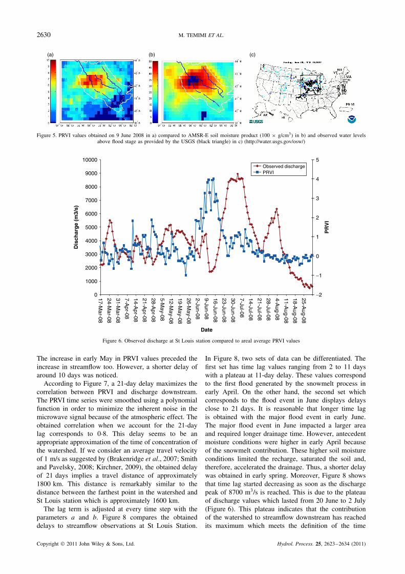
The extent of the areas displaying high PRVI valueswas assessed and compared to USGS records of riverdischarges above the flood stage and to AMSR-E standardsoil moisture product (Njoku et al., 2003). Figure 5ashows a PRVI map computed over the Upper MississippiRiver watershed on 9 June 2008 with a clear presence ofhigher PRVI values in the study area as a consequenceof the flood. Figure 5b presents the spatial distributionof soil moisture in the area obtained from the NASAAMSR-E product. Soil moisture was substantially high inupstream locations of the study area. Finally, Figure 5cdisplays the locations of water level above the floodstage in the Upper Mississippi watershed as reportedby the USGS on 9 June 2008 and shows that theseobservations were mainly located upstream. The spatialdistribution of high PRVI values is very similar to soilmoisture estimates from the AMSR-E product (Figure 5b). They also agree with the location of overbank flooding(Figure 5c). According to the spatial distribution of PRVI,extreme wetness conditions were more noticeable inupstream regions. PRVI values declined downstreamtowards Mississippi River. PRVI values were the highest,around eight, in the central part of the watershed. Thesevalues were higher than those obtained downstream.Figure 5b) shows few missing values in the central partof the watershed which are due to the presence ofintense precipitation. The PRVI map in Figure 5a doesnot show a similar gap because of the implementation



Table I. Total monthly rainfall observed at 8 stations (airports) in Iowa in 2008

Stations Latitude Longitude Monthly total (mm)

May June July

Des Moines international airport 41Ð538 �93Ð666 97Ð54 341Ð63 207Ð77Ames municipal airport 41Ð992 �93Ð622 210Ð31 267Ð97 202Ð95Iowa City municipal airport 41Ð663 �91Ð543 125Ð22 205Ð74 9Ð91Spencer municipal airport 43Ð164 �95Ð202 91Ð44 102Ð62 72Ð64Mason City municipal airport 43Ð158 �93Ð331 132Ð33 275Ð34 138Ð18Eppley airfield airport 41Ð31 �95Ð899 161Ð54 241Ð55 79Ð50Dubuque regional airport 42Ð398 �90Ð704 217Ð68 181Ð86 131Ð06Ottumwa industrial airport 41Ð107 �92Ð448 125Ð22 250Ð44 59Ð18

Figure 4. Observed total precipitation at eight sites in May, June, and July 2008 and their corresponding Thiessen polygons

of a compositing technique along with a threshold-basedapproach to systematically detect heavy rainy conditions.

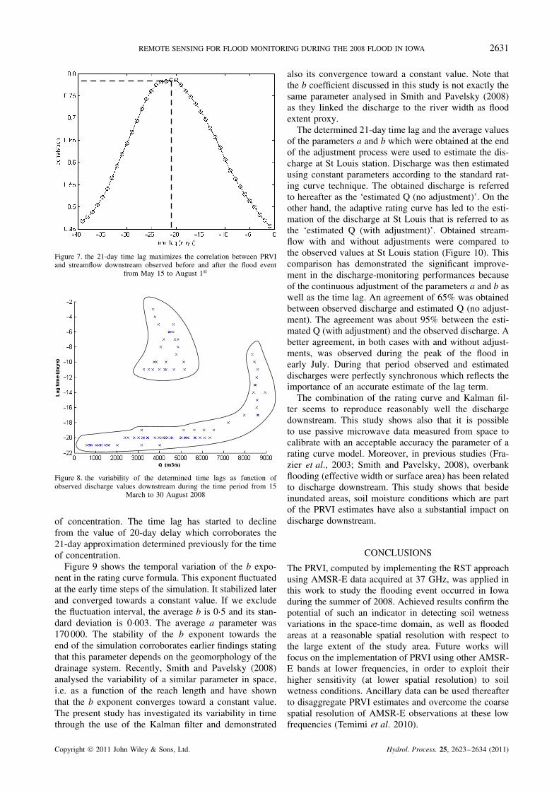
The temporal variation of areal average PRVI wascompared to streamflow in the Mississippi River atSt Louis station (Figure 6). Missouri and Illinois Rivers’streamflow, as well as streamflow observed at Clintonstation, were subtracted from St Louis station dischargeobservations to account only for contributions from theIowa watershed which are referred to, hereafter, as thedischarge at St Louis.

The difference in phase between the areal averagePRVI and discharge downstream is illustrated in Figure 6.The peak of PRVI has been observed on 9 June. On theother hand, the streamflow peak was recorded on 2 July,23 days later. Streamflow values have shown anotherincrease in early May. This increase is a consequenceof an earlier spring snowmelt which caused an increasein areal average PRVI in mid April. The discharge peakof 5660 m3/s recorded in early May was smaller thanthe observed 8700 m3/s peak during the flood event.



(a) (b) (c)

Figure 5. PRVI values obtained on 9 June 2008 in a) compared to AMSR-E soil moisture product (100 ð g/cm3) in b) and observed water levelsabove flood stage as provided by the USGS (black triangle) in c) (http://water.usgs.gov/osw/)

0

1000

2000

3000

4000

5000

6000

7000

8000

9000

10000

17-Mar-08

24-Mar-08

31-Mar-08

7-Apr-08

14-Apr-08

21-Apr-08

28-Apr-08

5-May-08

12-May-08

19-May-08

26-May-08

2-Jun-08

9-Jun-08

16-Jun-08

23-Jun-08

30-Jun-08

7-Jul-08

14-Jul-08

21-Jul-08

28-Jul-08

4-Aug-08

11-Aug-08

18-Aug-08

25-Aug-08

−2

−1

0

1

2

3

4

5

Date

Dis

char

ge

(m3/

s)

PR

VI

Observed dischargePRVI

Figure 6. Observed discharge at St Louis station compared to areal average PRVI values

The increase in early May in PRVI values preceded theincrease in streamflow too. However, a shorter delay ofaround 10 days was noticed.

According to Figure 7, a 21-day delay maximizes thecorrelation between PRVI and discharge downstream.The PRVI time series were smoothed using a polynomialfunction in order to minimize the inherent noise in themicrowave signal because of the atmospheric effect. Theobtained correlation when we account for the 21-daylag corresponds to 0Ð8. This delay seems to be anappropriate approximation of the time of concentration ofthe watershed. If we consider an average travel velocityof 1 m/s as suggested by (Brakenridge et al., 2007; Smithand Pavelsky, 2008; Kirchner, 2009), the obtained delayof 21 days implies a travel distance of approximately1800 km. This distance is remarkably similar to thedistance between the farthest point in the watershed andSt Louis station which is approximately 1600 km.

The lag term is adjusted at every time step with theparameters a and b. Figure 8 compares the obtaineddelays to streamflow observations at St Louis Station.

In Figure 8, two sets of data can be differentiated. Thefirst set has time lag values ranging from 2 to 11 dayswith a plateau at 11-day delay. These values correspondto the first flood generated by the snowmelt process inearly April. On the other hand, the second set whichcorresponds to the flood event in June displays delaysclose to 21 days. It is reasonable that longer time lagis obtained with the major flood event in early June.The major flood event in June impacted a larger areaand required longer drainage time. However, antecedentmoisture conditions were higher in early April becauseof the snowmelt contribution. These higher soil moistureconditions limited the recharge, saturated the soil and,therefore, accelerated the drainage. Thus, a shorter delaywas obtained in early spring. Moreover, Figure 8 showsthat time lag started decreasing as soon as the dischargepeak of 8700 m3/s is reached. This is due to the plateauof discharge values which lasted from 20 June to 2 July(Figure 6). This plateau indicates that the contributionof the watershed to streamflow downstream has reachedits maximum which meets the definition of the time



Figure 7. the 21-day time lag maximizes the correlation between PRVIand streamflow downstream observed before and after the flood event

from May 15 to August 1st

Figure 8. the variability of the determined time lags as function ofobserved discharge values downstream during the time period from 15

March to 30 August 2008

of concentration. The time lag has started to declinefrom the value of 20-day delay which corroborates the21-day approximation determined previously for the timeof concentration.

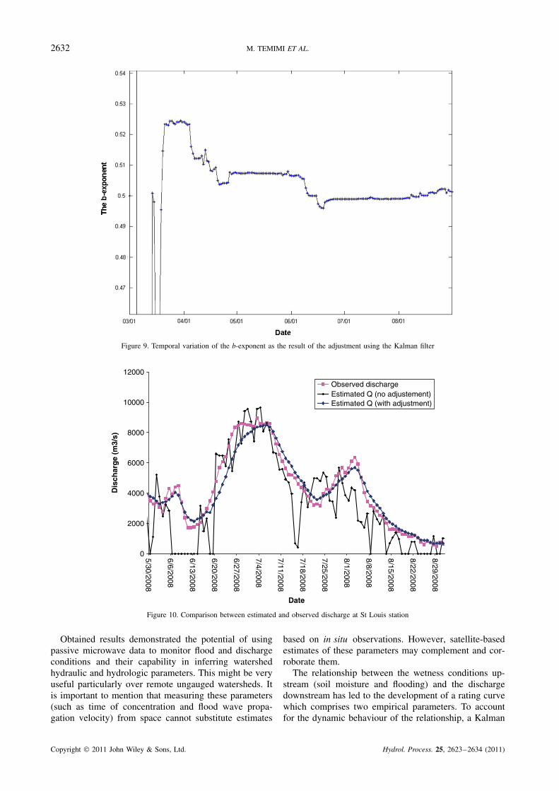
Figure 9 shows the temporal variation of the b expo-nent in the rating curve formula. This exponent fluctuatedat the early time steps of the simulation. It stabilized laterand converged towards a constant value. If we excludethe fluctuation interval, the average b is 0Ð5 and its stan-dard deviation is 0Ð003. The average a parameter was170 000. The stability of the b exponent towards theend of the simulation corroborates earlier findings statingthat this parameter depends on the geomorphology of thedrainage system. Recently, Smith and Pavelsky (2008)analysed the variability of a similar parameter in space,i.e. as a function of the reach length and have shownthat the b exponent converges toward a constant value.The present study has investigated its variability in timethrough the use of the Kalman filter and demonstrated

also its convergence toward a constant value. Note thatthe b coefficient discussed in this study is not exactly thesame parameter analysed in Smith and Pavelsky (2008)as they linked the discharge to the river width as floodextent proxy.

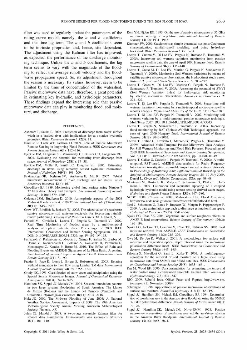
The determined 21-day time lag and the average valuesof the parameters a and b which were obtained at the endof the adjustment process were used to estimate the dis-charge at St Louis station. Discharge was then estimatedusing constant parameters according to the standard rat-ing curve technique. The obtained discharge is referredto hereafter as the ‘estimated Q (no adjustment)’. On theother hand, the adaptive rating curve has led to the esti-mation of the discharge at St Louis that is referred to asthe ‘estimated Q (with adjustment)’. Obtained stream-flow with and without adjustments were compared tothe observed values at St Louis station (Figure 10). Thiscomparison has demonstrated the significant improve-ment in the discharge-monitoring performances becauseof the continuous adjustment of the parameters a and b aswell as the time lag. An agreement of 65% was obtainedbetween observed discharge and estimated Q (no adjust-ment). The agreement was about 95% between the esti-mated Q (with adjustment) and the observed discharge. Abetter agreement, in both cases with and without adjust-ments, was observed during the peak of the flood inearly July. During that period observed and estimateddischarges were perfectly synchronous which reflects theimportance of an accurate estimate of the lag term.

The combination of the rating curve and Kalman fil-ter seems to reproduce reasonably well the dischargedownstream. This study shows also that it is possibleto use passive microwave data measured from space tocalibrate with an acceptable accuracy the parameter of arating curve model. Moreover, in previous studies (Fra-zier et al., 2003; Smith and Pavelsky, 2008), overbankflooding (effective width or surface area) has been relatedto discharge downstream. This study shows that besideinundated areas, soil moisture conditions which are partof the PRVI estimates have also a substantial impact ondischarge downstream.

CONCLUSIONS

The PRVI, computed by implementing the RST approachusing AMSR-E data acquired at 37 GHz, was applied inthis work to study the flooding event occurred in Iowaduring the summer of 2008. Achieved results confirm thepotential of such an indicator in detecting soil wetnessvariations in the space-time domain, as well as floodedareas at a reasonable spatial resolution with respect tothe large extent of the study area. Future works willfocus on the implementation of PRVI using other AMSR-E bands at lower frequencies, in order to exploit theirhigher sensitivity (at lower spatial resolution) to soilwetness conditions. Ancillary data can be used thereafterto disaggregate PRVI estimates and overcome the coarsespatial resolution of AMSR-E observations at these lowfrequencies (Temimi et al. 2010).



Figure 9. Temporal variation of the b-exponent as the result of the adjustment using the Kalman filter

0

2000

4000

6000

8000

10000

12000

5/30/2008

6/6/2008

6/13/2008

6/20/2008

6/27/2008

7/4/2008

7/11/2008

7/18/2008

7/25/2008

8/1/2008

8/8/2008

8/15/2008

8/22/2008

8/29/2008

Date

Dis

char

ge

(m3/

s)

Observed dischargeEstimated Q (no adjustement)Estimated Q (with adjustment)

Figure 10. Comparison between estimated and observed discharge at St Louis station

Obtained results demonstrated the potential of usingpassive microwave data to monitor flood and dischargeconditions and their capability in inferring watershedhydraulic and hydrologic parameters. This might be veryuseful particularly over remote ungauged watersheds. Itis important to mention that measuring these parameters(such as time of concentration and flood wave propa-gation velocity) from space cannot substitute estimates

based on in situ observations. However, satellite-basedestimates of these parameters may complement and cor-roborate them.

The relationship between the wetness conditions up-stream (soil moisture and flooding) and the dischargedownstream has led to the development of a rating curvewhich comprises two empirical parameters. To accountfor the dynamic behaviour of the relationship, a Kalman



filter was used to regularly update the parameters of therating curve model, namely, the a and b coefficientsand the time-lag term. The a and b coefficients seemto be intrinsic proprieties and, hence, site dependent.The adjustment using the Kalman filter has improved,as expected, the performance of the discharge monitor-ing technique. Unlike the a and b coefficients, the lagterm seems to vary with the magnitude of the flood-ing to reflect the average runoff velocity and the flood-wave propagation speed. So, its adjustment throughoutthe season is necessary. Its values, however, seem to belimited by the time of concentration of the watershed.Passive microwave data have, therefore, a great potentialin estimating key hydraulic, and hydrologic parameters.These findings expand the interesting role that passivemicrowave data can play in monitoring flood, soil mois-ture, and discharge.

REFERENCES

Ashmore P, Sauks E. 2006. Prediction of discharge from water surfacewidth in a braided river with implications for at-a-station hydraulicgeometry. Water Resources Research 42(3): 11.

Bindlish R, Crow WT, Jackson TJ. 2009. Role of Passive MicrowaveRemote Sensing in Improving Flood Forecasts. IEEE Geoscience andRemote Sensing Letters 6(1): 112–116.

Bjerklie DM, Dingman SL, Vorosmarty CJ, Bolster CH, Congalton RG.2003. Evaluating the potential for measuring river discharge fromspace. Journal of Hydrology 278(1): 17–38.

Bjerklie DM, Moller D, Smith LC, Dingman SL. 2005. Estimatingdischarge in rivers using remotely sensed hydraulic information.Journal of Hydrology 309(1): 191–209.

Brakenridge GR, Nghiem SV, Anderson E, Mic R. 2007. Orbitalmicrowave measurement of river discharge and ice status. WaterResources Research 43(4): 16.

Choudhury BJ. 1989. Monitoring global land surface using Nimbus-737 GHz data. Theory and examples. International Journal of RemoteSensing 10(10): 1579–1605.

Coleman JSM, Budikova D. 2010. Atmospheric aspects of the 2008Midwest floods: a repeat of 1993? International Journal of Climatology30(11): 1645–1667.

Crow WT, Bindlish R, Jackson TJ. 2005. The added value of spacebornepassive microwave soil moisture retrievals for forecasting rainfall-runoff partitioning. Geophysical Research Letters 32: L 18401, 5.

Faruolo M, Coviello I, Lacava T, Pergola N, Tramutoli V. 2009.Real Time Monitoring of flooded areas by a multi-temporalanalysis of optical satellite data. Proceedings of 2009 IEEEInternational Geoscience and Remote Sensing Symposium, Vol. 4,DOI:10.1109/IGARSS.2009.5417339, pp. IV-192–IV-195.

Ferrazzoli P, Rahmoune R, Moccia F, Grings F, Salvia M, Barber M,Douna V, Karszenbaum H, Soldano A, Goniadzki D, Parmuchi G,Montenegro C, Kandus P, Borro M. 2010. The Effect of Rain andFlooding Events on AMSR-E Signatures of La Plata Basin, Argentina.Ieee Journal of Selected Topics in Applied Earth Observations andRemote Sensing 3(1): 81–90.

Frazier P, Page K, Louis J, Briggs S, Robertson AI. 2003. Relatingwetland inundation to river flow using Landsat TM data. InternationalJournal of Remote Sensing 24(19): 3755–3770.

Grody NC. 1991. Classification of snow cover and precipitation using theSpecial Sensor Microwave Imager. Journal of Geophysical Research-Atmospheres 96(D4): 7423–7435.

Hamilton SK, Sippel SJ, Melack JM. 2004. Seasonal inundation patternsin two large savanna floodplains of South America: The Llanosde Moxos (Bolivia) and the Llanos del Orinoco (Venezuela andColombia). Hydrological Processes 18(11): 2103–2116.

Hoke JE. 2009. The Midwest Flooding of June 2008: A NationalWeather Service Assessment, Impacts of 2008. The 89th AmericanMeteorological Society Annual Meeting American MeteorologicalSociety: Phoenix, AZ.

Johns CJ, Mandel J. 2008. A two-stage ensemble Kalman filter forsmooth data assimilation. Environmental and Ecological Statistics15(1): 101–110.

Kerr YH, Njoku EG. 1993. On the use of passive microwaves at 37 GHzin remote sensing of vegetation. International Journal of RemoteSensing 14(10): 1931–1943.

Kirchner JW. 2009. Catchments as simple dynamical systems: Catchmentcharacterization, rainfall-runoff modeling, and doing hydrologybackward. Water Resources Research 45: 1–34.

Lacava T, Cuomo V, Di Leo EV, Pergola N, Romano F, Tramutoli V.2005a. Improving soil wetness variations monitoring from passivemicrowave satellite data: the case of April 2000 Hungary flood. RemoteSensing of Environment 96(2): 135–148.

Lacava T, Greco M, Di Leo EV, Martino G, Pergola N, Sannazzaro F.Tramutoli V. 2005b. Monitoring Soil Wetness variations by means ofsatellite passive microwave observations: the Hydroptimet study cases.Natural Hazards and Earth System Sciences 5: 583–592.

Lacava T, Greco M, Di Leo EV, Martino G, Pergola N, Romano F,Sannazzaro F, Tramutoli V. 2005c. Assessing the potential of SWVI(Soil Wetness Variation Index) for hydrological risk monitoringby satellite microwave observations. Advances in Geosciences 2:221–227.

Lacava T, Di Leo EV, Pergola N, Tramutoli V. 2006. Space-time soilwetness variations monitoring by a multi-temporal microwave satelliterecords analysis. Physics and Chemistry of the Earth 31: 1274–1283.

Lacava T, Di Leo, EV, Pergola N, Tramutoli V. 2007. Monitoring soilwetness variation by a multi-temporal passive microwave technique.MultiTemp 2007, DOI:10.1109/MULTITEMP.2007.4293043.

Lacava T, Pergola N, Sannazzaro F, Tramutoli V. 2009a. Improvingflood monitoring by RAT (Robust AVHRR Technique) approach: thecase of April 2000 Hungary flood. International Journal of RemoteSensing 31(18): 2043–2062.

Lacava T, Calice G, Coviello I, Mazzeo G, Pergola N, Tramutoli V.2009b. Advanced Multi-Temporal Passive Microwave Data AnalysisFor Soil Wetness Monitoring And Flood Risk Forecast. Proceedings of2009 IEEE International Geoscience and Remote Sensing Symposium,Vol. 3, DOI:10.1109/IGARSS.2009.5418299, pp. III-490–III-493.

Lacava T, Calice G, Coviello I, Pergola N, Tramutoli V. 2009c. A multi-temporal, RST-based, AMSR-E data analysis for Radio FrequencyInterference investigation: a possible impact on soil wetness retrievals.In Proceedings of Multitemp 2009, Fifth International Workshop on theAnalysis of Multitemporal Remote Sensing Images, 28–30 July 2009 ,Daniel L. Civco (ed), Mistic: Connecticut, USA; pp. 40–48.

Montanari M, Hostache R, Matgen P, Schumann G, Pfister L, Hoff-mann L. 2009. Calibration and sequential updating of a coupledhydrologic-hydraulic model using remote sensing-derived water stages.Hydrology and Earth System Sciences 13(3): 367–380.

NCDC. 2008. Climate of 2008; Midwestern U.S. Flood Overview,http://www.ncdc.noaa.gov/oa/climate/research/2008/flood08.html.

Neal J, Schumann G, Bates P, Buytaert W, Matgen P, Pappenberger F.2009. A data assimilation approach to discharge estimation from space.Hydrological Processes 23(25): 3641–3649.

Njoku EG, Chan SK. 2006. Vegetation and surface roughness effects onAMSR-E land observations. Remote Sensing of Environment 100(2):190–199.

Njoku EG, Jackson TJ, Lakshmi V, Chan TK, Nghiem SV. 2003. Soilmoisture retrieval from AMSR-E. IEEE Transactions on Geoscienceand Remote Sensing 41(2): 215–229.

Owe M, De Jeu R, Walker J. 2001. A methodology for surface soilmoisture and vegetation optical depth retrieval using the microwavepolarization difference index. IEEE Transactions on Geoscience andRemote Sensing 39(8): 1643–1654.

Paloscia S, Macelloni G, Santi E, Koike T. 2001. A multifrequencyalgorithm for the retrieval of soil moisture on a large scale usingmicrowave data from SMMR and SSM/I satellites. IEEE Transactionson Geoscience and Remote Sensing 39(8): 1655–1661.

Pan M, Wood EF. 2006. Data assimilation for estimating the terrestrialwater budget using a constrained ensemble Kalman filter. Journal ofHydrometeorology, 7(3): 534–547.

RIO. 2009. Rebuild Iowa Office, Facts and Figures, http://www.rio.iowa.gov, (11 November 2009).

Schmugge T. 1998. Applications of passive microwave observations ofsurface soil moisture. Journal of Hydrology 213(1): 188–197.

Sippel SJ, Hamilton SK, Melack JM, Choudhury BJ. 1994. Determina-tion of inundation area in the Amazon river floodplain using the SMMR37 GHz polarization difference. Remote Sensing of Environment 48(1):70–76.

Sippel SJ, Hamilton SK, Melack JM, Novo EMM. 1998. Passivemicrowave observations of inundation area and the area/stage relationin the Amazon River floodplain. International Journal of RemoteSensing 19(16): 3055–3074.



Smith LC, Isacks BL, Bloom AL. 1996. Estimation of discharge fromthree braided rivers using synthetic aperture radar satellite imagery:Potential application to ungaged basins. Water Resources Research32(7): 2021–2034.

Smith LC, Pavelsky TM. 2008. Estimation of river discharge,propagation speed, and hydraulic geometry from space: Lena River,Siberia. Water Resources Research 44(3): 1–11.

Tanaka M, Sugimura T, Tanaka S. 2000. Monitoring water surface ratioin the Chinese floods of summer 1998 by DMSP-SSM/I. InternationalJournal of Remote Sensing 21(8): 1561–1569.

Tanaka M, Sugimura T, Tanaka S, Tamai N. 2003. Flood-drought cycleof Tonle Sap and Mekong Delta area observed by DMSP-SSM/I.International Journal of Remote Sensing 24(7): 1487–1504.

Temimi M, Leconte R, Brissette F, Chaouch N. 2005. Flood monitoringover the Mackenzie River Basin using passive microwave data. RemoteSensing of Environment 98(2): 344–355.

Temimi M, Leconte R, Brissette F, Chaouch N. 2007. Flood and soilwetness monitoring over the Mackenzie River Basin using AMSR-E 37 GHz brightness temperature. Journal of Hydrology 333(2):317–328.

Temimi M, Ghedira H, Khanbilvardi R. 2009. Flood and discharge mon-itoring during the 2008 Iowa flood using AMSR-E data, Geoscience

and Remote Sensing Symposium, 2009. IEEE International, IGARSS2009, pp. V-280–V-283.

Temimi M, Leconte R, Chaouch N, Sukumal P, Khanbilvardi R, Bris-sette F. 2010. A combination of remote sensing data and topographicattributes for the spatial and temporal monitoring of soil wetness. Jour-nal of Hydrology 388(1): 28–40.

Tramutoli V. 2005. Robust Satellite Techniques (RST) for naturaland environmental hazards monitoring and mitigation: ten yearsof successful applications. In The 9th International Symposium onPhysical Measurements and Signatures in Remote Sensing , ShunlinLiang, Jiyuan Liu, Xiaowen Li, Ronggao Liu, Michael Schaepman(eds), ISPRS: Beijing (China); Vol. XXXVI (7/ W20), 792–795. ISSN1682–1750.

Tramutoli V. 2007. Robust Satellite Techniques (RST) for Natural andEnvironmental Hazards Monitoring and Mitigation: Theory and Appli-cations. MultiTemp 2007, DOI:10.1109/MULTITEMP.2007.4293057.

Wilheit T, Kummerow CD, Ferraro R. 2003. Rainfall algorithms forAMSR-E. IEEE Transactions on Geoscience and Remote Sensing41(2): 204–214.


Documents

A Multi-temporal Analysis of AMSR-E Data for Flood and