A Multi-Soft-Body Dynamic Model forUnderwater Soft Robots

Federico Renda, Francesco Giorgio-Serchi, Frederic Boyer, Cecilia Laschi, JorgeDias and Lakmal Seneviratne.

Abstract We present a unified formulation for describing the dynamics of a newclass of aquatic multi-body soft robots. This formulation accounts for the continuumhyperelastic nature of the vehicles and for the interaction with the dense fluid acrosswhich they dwell. We start by introducing the highly unconventional design conceptof a soft underwater vehicle inspired by the octopus capable of swimming, manip-ulating and crawling. The dynamics of the robot, which consists of a multi-limbedcontinuum of elastomeric materials, is extremely complex to account for with con-ventional modelling tools. Hence a Cosserat based formalism where a Reissner shellmodel and a finite-strain beam formulation are joined is conceived which lends itselfto the description of the highly non linear dynamics of this new family of vehiclesin a dense fluid.

1 Introduction

Marine operations and the growing needs of the offshore industry require underwa-ter robots to undertake increasingly daunting tasks in always more forbidding envi-ronments. Certain scenarios, however, pose such challenges at sea that standard Re-motely Operated Vehicles (ROVs) and Autonomous Underwater Vehicles (AUVs)are likely to be unsuitable. An answer to this problem lies in the development of in-

F. Renda, J. Dias, L. SeneviratneKURI, Khalifa University, Abu Dhabi, UAE.e-mail: federico.renda@kustar.ac.ae; jorge.dias@kustar.ac.ae; lakmal.seneviratne@kustar.ac.ae

F. Giorgio Serchi, C. Laschithe BioRobotics Institute, Scuola Superiore Sant’Anna, Pisa, Italy. e-mail: f.serchi@sssup.it; ce-cilia.laschi@sssup.it

F. BoyerIRCCyN, Ecole de Mines de Nantes, Nantes, France. e-mail: frederic.boyer@mines-nantes.fr

1

2 F. Renda et al

novative underwater robots which, endowed with augmented manoeuvrability andflexibility, may provide an aid to the ever growing demands of the marine sector.

In recent times underwater robotics has largely benefited from the growing fas-cination for bioinspired locomotion, because the design of underwater robots canprofit massively from the investigation of the swimming strategies, hydrodynamicsand physiology of such animals. Several examples exist of aquatic organisms whichhave been taken as the source of inspiration for designing a trustworthy roboticcounterpart. The finned and caudal flapping of fish (e.g. [1]) has gathered the mostrecognition in the scientific community, in part because of the sound understandingof the underlying physics involved in their locomotion [2].

The design criteria for replicating the actuation mechanism which drives thepropulsion of fish has, in most cases, entailed the replacement of continuously de-forming bodies by reducing the number of degrees-of-freedom (DOF) with a finitesequence of rigid links and joints. However, lately the attempt has been made by[3] to account for the compliant nature of these organisms by resorting to continu-ous soft structures and actuators. This is one of the few examples where the designprinciples of soft robotics [4] have been adapted to the aquatic context. In waterthe hindrances due to the lack of rigid parts are compensated by the support of thedense medium in which the vehicle is immersed, annihilating many of the limitswhich soft robots are faced with on land. This has encouraged the authors to de-velop a new breed of aquatic soft robots inspired by the quintessential soft-bodiedsea dweller, the octopus.

While the design of Soft Unmanned Underwater Vehicles (SUUVs), may resultfairly uncomplicated, their modeling and control is anything but straight forward.Here we present the first example of a cable-actuated, multi-body, aquatic soft robotand introduce a formulation which accounts for the continuum nature of the roboticplatform and allows to describe the dynamics of this vehicle while it travels in aquiescent fluid.

1.1 An aquatic multi-body soft robot

The octopus sports a range of features which are very much sought for in underwaterrobotics. These include essentially the capability to swim, crawl and manipulatealong with an overall remarkable structural compliance. These make the octopusthe perfect paradigm of aquatic vehicle. In the scenario of offshore intervention,where complex environments and highly perturbed conditions are the norm, thedesign criteria borrowed from the soft/bioinspired approach could represent a viablesolution to a broad range of tasks which current Unmanned Underwater Vehicles(UUVs) are unfit for.

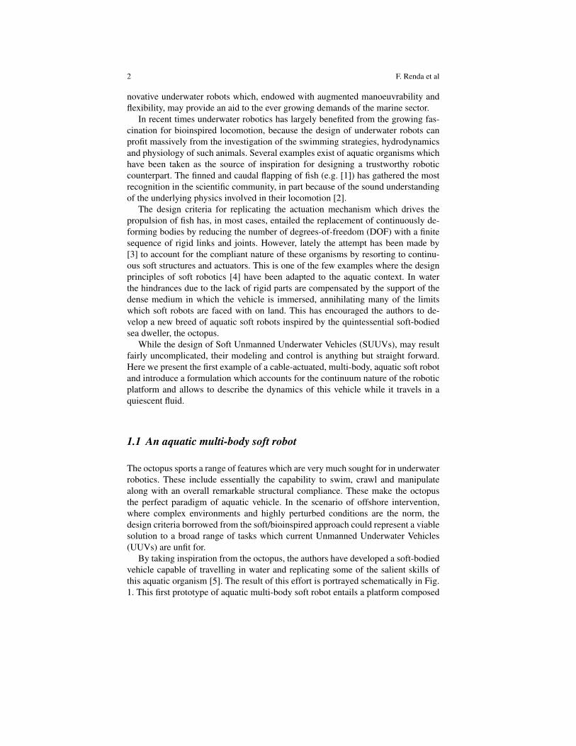
By taking inspiration from the octopus, the authors have developed a soft-bodiedvehicle capable of travelling in water and replicating some of the salient skills ofthis aquatic organism [5]. The result of this effort is portrayed schematically in Fig.1. This first prototype of aquatic multi-body soft robot entails a platform composed

A Multi-Soft-Body Dynamic Model for Underwater Soft Robots 3

Fig. 1 A schematic of theSUUV developed by the au-thors. Numbers refer to: (1)pulsed-jet thruster, (2) thenozzle, (3) the cables whichdrive the shell collapse, (4)the continuum manipulators,(5) the actutors of the manip-ulators, (6) the actuator of theshell and (7) the cable whichdrives manipulator actuation.

3

4

12

5 6 7

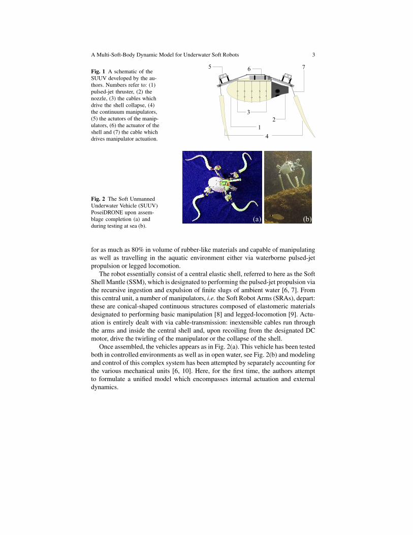
Fig. 2 The Soft UnmannedUnderwater Vehicle (SUUV)PoseiDRONE upon assem-blage completion (a) andduring testing at sea (b).

(a) (b)

for as much as 80% in volume of rubber-like materials and capable of manipulatingas well as travelling in the aquatic environment either via waterborne pulsed-jetpropulsion or legged locomotion.

The robot essentially consist of a central elastic shell, referred to here as the SoftShell Mantle (SSM), which is designated to performing the pulsed-jet propulsion viathe recursive ingestion and expulsion of finite slugs of ambient water [6, 7]. Fromthis central unit, a number of manipulators, i.e. the Soft Robot Arms (SRAs), depart:these are conical-shaped continuous structures composed of elastomeric materialsdesignated to performing basic manipulation [8] and legged-locomotion [9]. Actu-ation is entirely dealt with via cable-transmission: inextensible cables run throughthe arms and inside the central shell and, upon recoiling from the designated DCmotor, drive the twirling of the manipulator or the collapse of the shell.

Once assembled, the vehicles appears as in Fig. 2(a). This vehicle has been testedboth in controlled environments as well as in open water, see Fig. 2(b) and modelingand control of this complex system has been attempted by separately accounting forthe various mechanical units [6, 10]. Here, for the first time, the authors attemptto formulate a unified model which encompasses internal actuation and externaldynamics.

4 F. Renda et al

2 Soft Robot Arm and Soft Shell Mantle Model

In the geometrical exact approach, the SRA is viewed as a Cosserat rod [11], i.e.as a continuous assembly of rigid cross section, while the SSM is modelled as aCosserat axisymetric shell [12], i.e. as a continuous assembly of fibers along themedian surface. In this section, a brief description of the kinematics and dynamicsof a Cosserat rod/shell for underwater soft robotics is given, based on the authorsprevious works [8], [13], which should be taken as the reference for a more detailedderivation. Experimental validation of the model are also presented in [8] for theSRA, while for the SSM steady state experiments have been presented in [14], dy-namic experiments are under review and a coupled dynamic-potential flow solutionis given in [15]. In order to appreciate the symmetry between the two models, with aslight abuse of notation, some times we will adopt the same symbols for the two for-mulations, since they share the same geometrical and mechanical meaning in boththe cases.

2.1 Kinematics

The reference space is endowed with a base of orthogonal unit vectors (e1,e2,e3)(Fig. 3). In the Cosserat theory, the configuration of a soft body at a certain timeis characterized by a position vector r and a material orientation matrix R, param-eterized by the material abscissas, that are φ ∈ [0,2π[, the angle of revolution ofthe axisymmetric surface, and X ∈ [0,Ls] the abscissa along the meridian for theSSM; and X ∈ [0,Lb], the abscissa along the robot arm, for the SRA (the subscriptss and b stand respectively for shell and beam). Thus, the configuration space is de-

fined as a curves gb(X) and a surface gs(X ,φ) ∈ SE(3), with gb =

(Rb rb0 1

)and

gs =

(Rs rs0 1

).

In order to exploit the axisymmetry of the SSM, we introduce another orthogo-nal basis attached to the material point (X ,φ): (er,eφ ,e3) (Fig. 3); defined by roto-

traslating (e1,e2,e3) of g1(X ,φ) equal to: g1 =

(exp(e3φ) rs

0 1

), where exp is the

exponential in SO(3). In this case rs(X) take the form: rs = (cos(φ)r,sin(φ)r,z)T

for which, r(X) and z(X) are two smooth functions which define the radius andthe altitude of the point X on the profile (Fig. 3). For the sake of convenience,we introduce another orthogonal basis (er,e3,−eφ ) rotated from the former by

g2 =

(exp(erπ/2) 0

0 1

). Then, if we call θ(X) the angle between e3 and the shell

fiber located at any X along the φ -meridian, the so called director orthogonal frame

(x,y,z) is defined at each instant t, by g3(X) equal to: g3 =

(exp(−eφ θ) 0

0 1

). Fi-

nally, putting them all together, the shell configuration space is gs = g1g2g3.

A Multi-Soft-Body Dynamic Model for Underwater Soft Robots 5

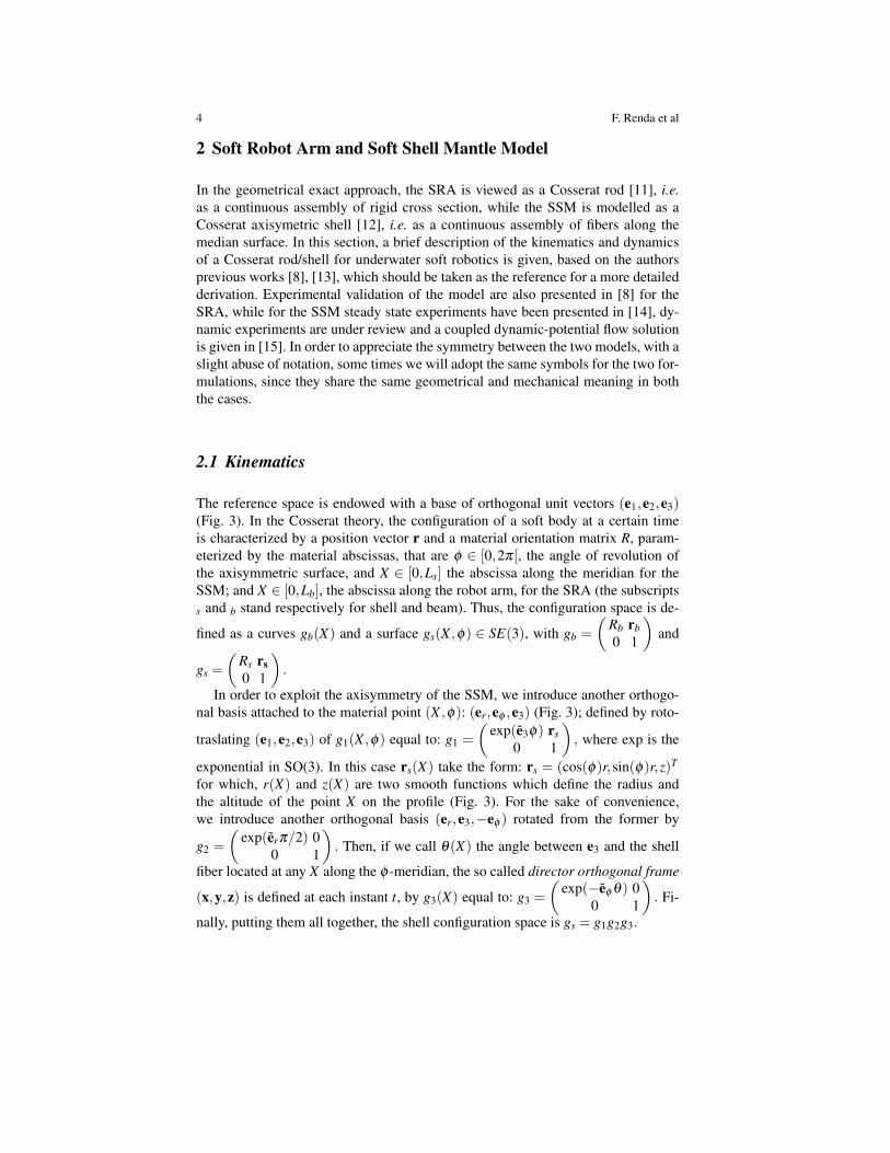
Fig. 3 Sketch of the kinemat-ics which show the geometri-cal meaning of the elementsg, ξ and η . The referenceframes on the figure are thoseused in the model.

Now, the tangent vector field along the curve gb(X) is defined by ξ (X) =g−1

b ∂gb/∂X = g−1b g′b ∈ se(3) and the tangent plane on the surface gs(X ,φ) is defined

by the two vector fields: ξ1(X)= g−1s ∂gs/∂X = g−1

s g′s and ξ2(X)= g−1s ∂gs/∂ (r?φ)=

g−1s gos (where ? denote variable in the reference configuration). In local frame

components we have: ξ = (kT ,gT )T , ξ1 = (kT1 ,g

T1 )

T = (0,0,µ,λ ,β ,0)T , ξ2 =

(kT2 ,g

T2 )

T = ( sin(θ)r? , cos(θ)

r? ,0,0,0,− rr? )

T ∈ R6. where g(X) represents the linearstrains, and k(X) the angular strain. The hat is the isomorphism between the twistvector space R6 and the Lie algebra se(3).

The time evolution of the configuration curve gb and surface gs is represented bythe twist vector field η(X) ∈ R6 defined respectively by ηb = g−1

b ∂gb/∂ t = g−1b gb

and ηs = g−1s ∂gs/∂ t = g−1

s gs. As before, in the local components we have: ηb =(wT

b ,vTb )

T , ηs = (wTs ,v

Ts )

T = (0,0,Ω ,Vx,Vy,0)T ∈ R6, where v(X) and w(X) arerespectively the linear and angular velocity of a material element at a given instant.

In accordance with this kinematics, the state vector of the SRA and of the SSMare represented by the terns (gb,ξ ,ηb) and (gs,ξ1,ηs). From the development above,we can derived the kinematic equations (1) and (2), while in the next sections thecompatibility equations and the dynamic equations will be derived (the tilde is theisomorphism between a vector of R3 and the corresponding skew-symmetric matrix∈ so(3)).

rb = RbvbaaaaaaRb = Rbwb. (1)

θ = Ω

r = cos(θ)Vx− sin(θ)Vyz = sin(θ)Vx + cos(θ)Vy

(2)

2.2 Strain Measures

There are different ways to measure the strain of a continuous media, we choose themost common used in the specialized literature for the beam and shell separately.

6 F. Renda et al

For the SRA, the strains are defined as the difference between the deformed con-figuration ξ and the reference configuration ξ ?. In particular, the components ofk−k? measure the torsion and the bending state in the two directions. Similarly, thecomponents of g−g? represent the longitudinal strain (extension, compression) andthe two shear strains.

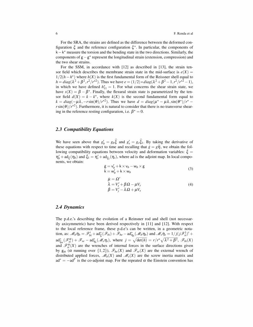
For the SSM, in accordance with [12] as described in [13], the strain ten-sor field which describes the membrane strain state in the mid-surface is e(X) =1/2(h−h?) where h(X) is the first fundamental form of the Reissner shell equal toh = diag(λ 2 +β 2,r2/r?2). Thus we have e = (1/2)∗diag(λ 2 +β 2−1,r2/r?2−1),in which we have defined h?11 = 1. For what concerns the shear strain state, wehave s(X) = β − β ?. Finally, the flexural strain state is parametrized by the ten-sor field d(X) = k − k?, where k(X) is the second fundamental form equal tok = diag(−µλ ,−r sin(θ)/r?2). Thus we have d = diag(µ? − µλ ,sin(θ ?)/r? −r sin(θ)/r?2). Furthermore, it is natural to consider that there is no transverse shear-ing in the reference resting configuration, i.e. β ? = 0.

2.3 Compatibility Equations

We have seen above that g′b = gbξ and g′s = gsξ1. By taking the derivative ofthese equations with respect to time and recalling that g = gη , we obtain the fol-lowing compatibility equations between velocity and deformation variables: ξ =η ′b + adξ (ηb) and ξ1 = η ′s + adξ1

(ηs), where ad is the adjoint map. In local compo-nents, we obtain:

g = v′b +k×vb−wb×gk= w′b +k×wb

(3)

µ = Ω ′

λ =V ′x +βΩ −µVy

β =V ′y −λΩ +µVx

(4)

2.4 Dynamics

The p.d.e.’s describing the evolution of a Reinsner rod and shell (not necessar-ily axisymmetric) have been derived respectively in [11] and [12]. With respectto the local reference frame, these p.d.e’s can be written, in a geometric nota-tion, as: Mbηb = F ′

bi + ad∗ξ(Fbi)+Fbe− ad∗ηb

(Mbηb) and Msηs = 1/ j( jF 1si)′+

ad∗ξα(F α

si ) + Fse − ad∗ηs(Msηs), where j =√

det(h) = r/r?√

λ 2 +β 2, Fbi(X)

and F αsi (X) are the wrenches of internal forces in the surface directions given

by gα (α running over 1,2), Fbe(X) and Fse(X) are the external wrench ofdistributed applied forces, Mb(X) and Ms(X) are the screw inertia matrix andad∗ = −adT is the co-adjoint map. For the repeated α the Einstein convention has

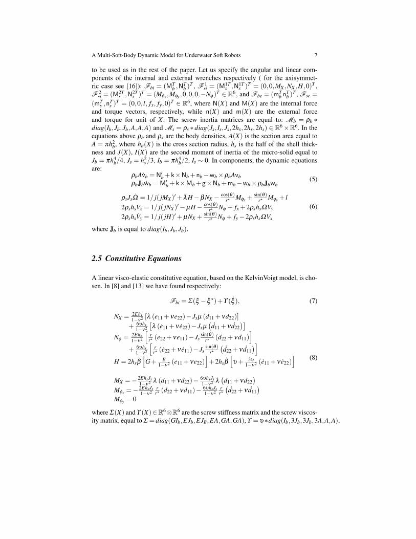
A Multi-Soft-Body Dynamic Model for Underwater Soft Robots 7

to be used as in the rest of the paper. Let us specify the angular and linear com-ponents of the internal and external wrenches respectively ( for the axisymmet-ric case see [16]): Fbi = (MT

b ,NTb )

T , F 1si = (M1T

s ,N1Ts )T = (0,0,MX ,NX ,H,0)T ,

F 2si = (M2T

s ,N2Ts )T = (Mφx ,Mφy ,0,0,0,−Nφ )

T ∈ R6, and Fbe = (mTb n

Tb )

T , Fse =

(mTs ,n

Ts )

T = (0,0, l, fx, fy,0)T ∈ R6, where N(X) and M(X) are the internal forceand torque vectors, respectively, while n(X) and m(X) are the external forceand torque for unit of X . The screw inertia matrices are equal to: Mb = ρb ∗diag(Ib,Jb,Jb,A,A,A) and Ms = ρs ∗ diag(Js, Is,Js,2hs,2hs,2hs) ∈ R6×R6. In theequations above ρb and ρs are the body densities, A(X) is the section area equal toA = πh2

b, where hb(X) is the cross section radius, hs is the half of the shell thick-ness and J(X), I(X) are the second moment of inertia of the micro-solid equal toJb = πh4

b/4, Js = h2s/3, Ib = πh4

b/2, Is ∼ 0. In components, the dynamic equationsare:

ρbAvb = N′b +k×Nb +nb−wb×ρbAvbρbJbwb =M′b +k×Mb +g×Nb +mb−wb×ρbJbwb

(5)

ρsJsΩ = 1/ j( jMX )′+λH−βNX − cos(θ)

r? Mφx +sin(θ)

r? Mφy + l2ρshsVx = 1/ j( jNX )

′−µH− cos(θ)r? Nφ + fx +2ρshsΩVy

2ρshsVy = 1/ j( jH)′+µNX + sin(θ)r? Nφ + fy−2ρshsΩVx

(6)

where Jb is equal to diag(Ib,Jb,Jb).

2.5 Constitutive Equations

A linear visco-elastic constitutive equation, based on the KelvinVoigt model, is cho-sen. In [8] and [13] we have found respectively:

Fbi = Σ(ξ −ξ?)+ϒ (ξ ), (7)

NX = 2Ehs1−ν2 [λ (e11 +νe22)− Jsµ (d11 +νd22)]

aaaa+ 6υhs1−ν2

[λ (e11 +ν e22)− Jsµ

(d11 +ν d22

)]Nφ = 2Ehs

1−ν2

[rr? (e22 +νe11)− Js

sin(θ)r? (d22 +νd11)

]aaaa+ 6υhs

1−ν2

[rr? (e22 +ν e11)− Js

sin(θ)r?(d22 +ν d11

)]H = 2hsβ

[G+ E

1−ν2 (e11 +νe22)]+2hsβ

[υ + 3υ

1−ν2 (e11 +ν e22)]

MX =− 2EhsJs1−ν2 λ (d11 +νd22)− 6υhsJs

1−ν2 λ(d11 +ν d22

)Mφx =−

2EhsJs1−ν2

rr? (d22 +νd11)− 6υhsJs

1−ν2rr?(d22 +ν d11

)Mφy = 0

(8)

where Σ(X) andϒ (X)∈R6⊗R6 are the screw stiffness matrix and the screw viscos-ity matrix, equal to Σ = diag(GIb,EJb,EJB,EA,GA,GA),ϒ =υ ∗diag(Ib,3Jb,3Jb,3A,A,A),

8 F. Renda et al

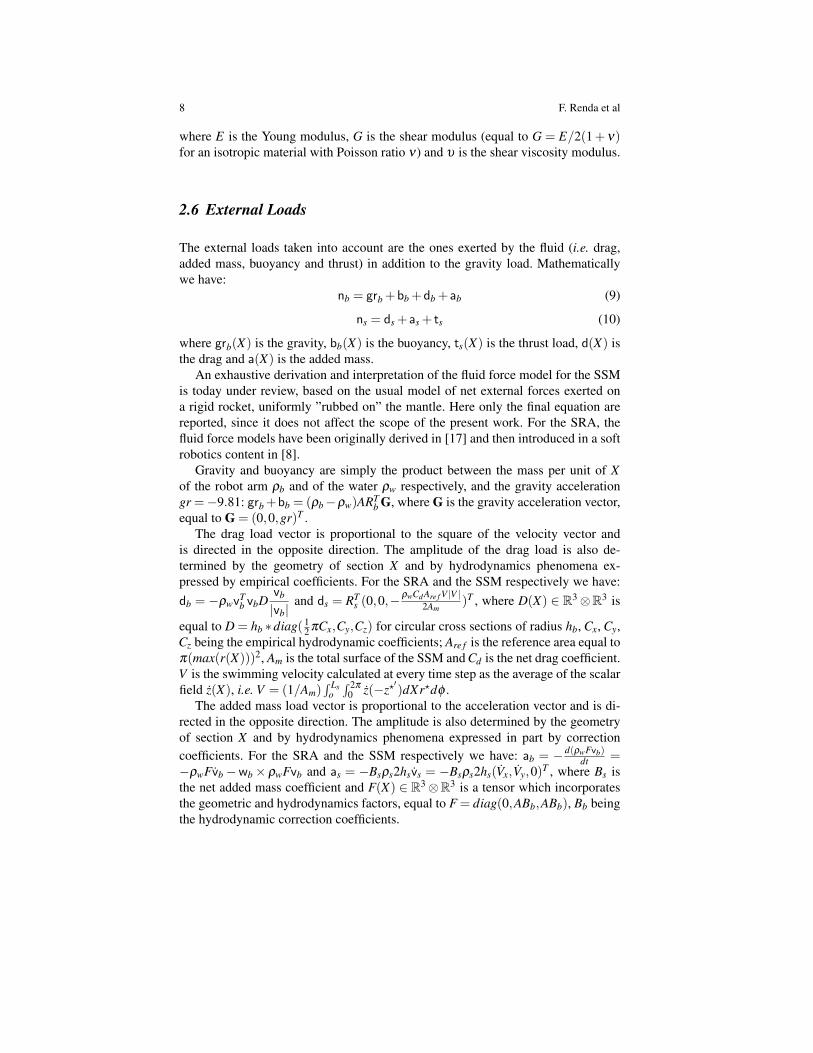
where E is the Young modulus, G is the shear modulus (equal to G = E/2(1+ν)for an isotropic material with Poisson ratio ν) and υ is the shear viscosity modulus.

2.6 External Loads

The external loads taken into account are the ones exerted by the fluid (i.e. drag,added mass, buoyancy and thrust) in addition to the gravity load. Mathematicallywe have:

nb = grb +bb +db +ab (9)

ns = ds +as + ts (10)

where grb(X) is the gravity, bb(X) is the buoyancy, ts(X) is the thrust load, d(X) isthe drag and a(X) is the added mass.

An exhaustive derivation and interpretation of the fluid force model for the SSMis today under review, based on the usual model of net external forces exerted ona rigid rocket, uniformly ”rubbed on” the mantle. Here only the final equation arereported, since it does not affect the scope of the present work. For the SRA, thefluid force models have been originally derived in [17] and then introduced in a softrobotics content in [8].

Gravity and buoyancy are simply the product between the mass per unit of Xof the robot arm ρb and of the water ρw respectively, and the gravity accelerationgr =−9.81: grb+bb = (ρb−ρw)ART

b G, where G is the gravity acceleration vector,equal to G = (0,0,gr)T .

The drag load vector is proportional to the square of the velocity vector andis directed in the opposite direction. The amplitude of the drag load is also de-termined by the geometry of section X and by hydrodynamics phenomena ex-pressed by empirical coefficients. For the SRA and the SSM respectively we have:db = −ρwv

Tb vbD

vb

|vb|and ds = RT

s (0,0,−ρwCdAre f V |V |

2Am)T , where D(X) ∈ R3⊗R3 is

equal to D = hb ∗diag( 12 πCx,Cy,Cz) for circular cross sections of radius hb, Cx, Cy,

Cz being the empirical hydrodynamic coefficients; Are f is the reference area equal toπ(max(r(X)))2, Am is the total surface of the SSM and Cd is the net drag coefficient.V is the swimming velocity calculated at every time step as the average of the scalarfield z(X), i.e. V = (1/Am)

∫ Lso∫ 2π

0 z(−z?′)dXr?dφ .

The added mass load vector is proportional to the acceleration vector and is di-rected in the opposite direction. The amplitude is also determined by the geometryof section X and by hydrodynamics phenomena expressed in part by correctioncoefficients. For the SRA and the SSM respectively we have: ab = − d(ρwFvb)

dt =−ρwFvb−wb× ρwFvb and as = −Bsρs2hsvs = −Bsρs2hs(Vx,Vy,0)T , where Bs isthe net added mass coefficient and F(X) ∈ R3⊗R3 is a tensor which incorporatesthe geometric and hydrodynamics factors, equal to F = diag(0,ABb,ABb), Bb beingthe hydrodynamic correction coefficients.

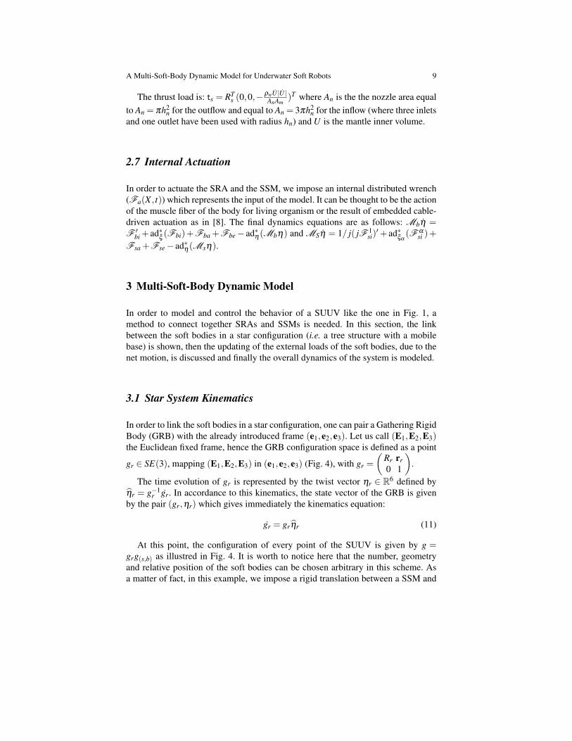
A Multi-Soft-Body Dynamic Model for Underwater Soft Robots 9

The thrust load is: ts = RTs (0,0,−

ρwU |U |AnAm

)T where An is the the nozzle area equalto An = πh2

n for the outflow and equal to An = 3πh2n for the inflow (where three inlets

and one outlet have been used with radius hn) and U is the mantle inner volume.

2.7 Internal Actuation

In order to actuate the SRA and the SSM, we impose an internal distributed wrench(Fa(X , t)) which represents the input of the model. It can be thought to be the actionof the muscle fiber of the body for living organism or the result of embedded cable-driven actuation as in [8]. The final dynamics equations are as follows: Mbη =F ′

bi + ad∗ξ(Fbi)+Fba +Fbe− ad∗η(Mbη) and MSη = 1/ j( jF 1

si)′+ ad∗

ξα(F α

si )+

Fsa +Fse− ad∗η(Msη).

3 Multi-Soft-Body Dynamic Model

In order to model and control the behavior of a SUUV like the one in Fig. 1, amethod to connect together SRAs and SSMs is needed. In this section, the linkbetween the soft bodies in a star configuration (i.e. a tree structure with a mobilebase) is shown, then the updating of the external loads of the soft bodies, due to thenet motion, is discussed and finally the overall dynamics of the system is modeled.

3.1 Star System Kinematics

In order to link the soft bodies in a star configuration, one can pair a Gathering RigidBody (GRB) with the already introduced frame (e1,e2,e3). Let us call (E1,E2,E3)the Euclidean fixed frame, hence the GRB configuration space is defined as a point

gr ∈ SE(3), mapping (E1,E2,E3) in (e1,e2,e3) (Fig. 4), with gr =

(Rr rr0 1

).

The time evolution of gr is represented by the twist vector ηr ∈ R6 defined byηr = g−1

r gr. In accordance to this kinematics, the state vector of the GRB is givenby the pair (gr,ηr) which gives immediately the kinematics equation:

gr = grηr (11)

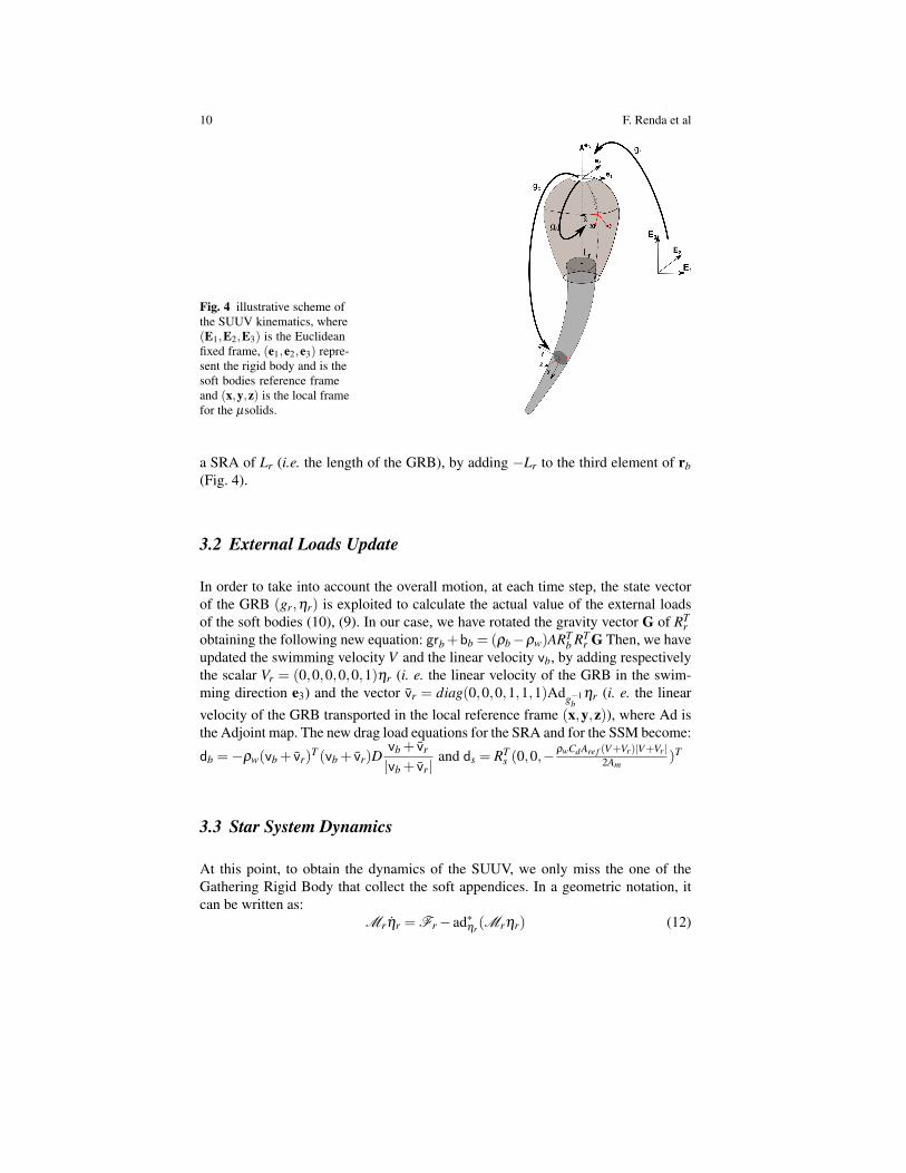
At this point, the configuration of every point of the SUUV is given by g =grg(s,b) as illustred in Fig. 4. It is worth to notice here that the number, geometryand relative position of the soft bodies can be chosen arbitrary in this scheme. Asa matter of fact, in this example, we impose a rigid translation between a SSM and

10 F. Renda et al

Fig. 4 illustrative scheme ofthe SUUV kinematics, where(E1,E2,E3) is the Euclideanfixed frame, (e1,e2,e3) repre-sent the rigid body and is thesoft bodies reference frameand (x,y,z) is the local framefor the µsolids.

a SRA of Lr (i.e. the length of the GRB), by adding −Lr to the third element of rb(Fig. 4).

3.2 External Loads Update

In order to take into account the overall motion, at each time step, the state vectorof the GRB (gr,ηr) is exploited to calculate the actual value of the external loadsof the soft bodies (10), (9). In our case, we have rotated the gravity vector G of RT

robtaining the following new equation: grb+bb = (ρb−ρw)ART

b RTr G Then, we have

updated the swimming velocity V and the linear velocity vb, by adding respectivelythe scalar Vr = (0,0,0,0,0,1)ηr (i. e. the linear velocity of the GRB in the swim-ming direction e3) and the vector vr = diag(0,0,0,1,1,1)Adg−1

bηr (i. e. the linear

velocity of the GRB transported in the local reference frame (x,y,z)), where Ad isthe Adjoint map. The new drag load equations for the SRA and for the SSM become:

db =−ρw(vb + vr)T (vb + vr)D

vb + vr

|vb + vr|and ds = RT

s (0,0,−ρwCdAre f (V+Vr)|V+Vr |

2Am)T

3.3 Star System Dynamics

At this point, to obtain the dynamics of the SUUV, we only miss the one of theGathering Rigid Body that collect the soft appendices. In a geometric notation, itcan be written as:

Mrηr = Fr− ad∗ηr(Mrηr) (12)

A Multi-Soft-Body Dynamic Model for Underwater Soft Robots 11

The soft bodies of the SUUV collected together by the GRB, are frozen in their cur-rent shape. By taking advantage of that, the above unknown parameters (Mr,Fr)

can be calculated as follow ([18]): Mr =∫ 2π

0∫ Ls

0 Ad∗gsMsAdg−1s(−z?

′)dXr?dφ +∫ Lb

0 Ad∗gbMbAdg−1

bdX+Mri =M ′

s +M ′b+Mri and Fr =

∫ 2π

0∫ Ls

0 Ad∗gsFse(−z′)dXrdφ +∫ Lb0 Ad∗gb

Fbe√gTgdX +Fre = F ′

se +F ′be +Fre, where Mri and Fre are respec-

tively the intrinsic inertia and external load directly belonging to the GRB, andAd∗g = (Adg)

−T is the coAdjoint map. It is worth to notice that the internal reactionand actuation of the soft bodies does not take part of these integrals, since a frozenshape have to be considered. Furthermore, as a first approximation, the inertia loadsdue to the ralitive acceleration of the soft bodies has not been taken into account. Thecontribute of the added mass loads of the soft bodies in F ′

se and F ′be will appear as

an additional mass as follow: M ′sa =Bsρs2h

∫ 2π

0∫ Ls

0 Ad∗gs diag(0,0,0,1,1,1)Adg−1s(−z?

′)dXr?dφ

and M ′ba = BbρwA

∫ Lb0 Ad∗gb

diag(0,0,0,0,1,1)Adg−1b

dX .Going forward into details, in our case, the intrinsic inertia of the GRB is equal

to Mri = ρrUr

(diag(Jr,Jr, Ir) u

uT diag(1,1,1)

), where u= (0,0,−3Lr/4)T is the po-

sition vector of the center of mass of the GRB whit respect to the reference frame(e1,e2,e3); Jr, Ir are the second moment of inertia equal to Jr = 3(h2

r/4+ L2r )/5,

Ir = 3h2r/10 (a conic shape have been chosen with base radius hr), ρr is the density

and Ur is the volume of the rigid body equal to Ur = πh2r Lr/3. On the other side,

the external loads on the GRB that have been considered are the gravity and buoy-ancy of the rigid body as well as the gravity and buoyancy of the SSM, since theletter have not been taken into account for the axisymmetric model. Thus we have:Fre = [(1−ρw/ρr)Mri +(1−ρw/ρs)M ′

s ]Adg−1r(0,0,0,GT )T .

3.4 SUUV Dynamic Model

The final system of equations is composed by the second order partial differen-tial equations of the soft bodies and the ordinary differential equations of the starsystem. The system of p.d.e.’s is composed by the kinematics equation (2), (1),the compatibility equations (4), (3) and the dynamic equations (6), (5) respectivelycomplemented with the internal stresses (8), (7) and the external loads (10), (9).The system of o.d.e.’s for the star system is composed by the kinematic equation(11) and the dynamic equation (12). Finally, in the state form x = f (x,x′,x′′, t), theSUUV model is:

12 F. Renda et al

θ = Ω

r = cos(θ)Vx− sin(θ)Vyz = sin(θ)Vx + cos(θ)Vyrb = RbvbRb = Rbwbgr = grηrµ = Ω ′

λ =V ′x +βΩ −µVy

β =V ′y −λΩ +µVx

k= w′b +k×wbg = v′b +k×vb−wb×gΩ = [( jMX )

′/ j+λH−βNX − cos(θ)Mφ/r?]/(ρJs)Vx = [( jNX )

′/ j−µH− cos(θ)Nφ/r?+2ρshsΩVy + fx]/[2hsρs(1+Bs)]Vy = [( jH)′/ j+µNX + sin(θ)Nφ/r?−2ρshsΩVx + fy]/[2hsρs(1+Bs)]vb = (N′b +k×Nb +nb−wb×ρbAvb)/(ρbA)wb = (J−1

b /ρb)(M′b +k×Mb +g×Nb +mb−wb×ρbJbwb)

ηr = M−1r [Fr− ad∗ηr(Mrηr)]

(13)

The final system is infinite dimensional since all its components are some func-tions of the profile abscissa X . As a result, in order to be solved numerically, ithas to be first space-discretised on a grid of nodes before being time integrated us-ing explicit or implicit time integrators starting from the initial state. In this grid,all the space derivatives appearing in the p.d.e.’s system can be approximated byfinite difference schemes, with the following boundary conditions: η(0) = 0 andFbi(Lb) = F 1

si(Ls) = 0. These operations have been implemented in Matlab c©.

4 Results

Although the final goal of this work is to model and control SUUVs like the one inFig. 1, whereby experimental comparison are needed (as has been done separatelyfor the SRA [8] and for the SSM [14]), in this section an illustrative example, basedon simulation, of the setting developed above is presented, in order to demonstratethe feasibility of the proposed mathematical framework to achieve the objective.Further simulation analysis and experimental comparisons with the real prototype,are planned for the extension of the present paper. Finally, an energetic analysisdisclosed by the current formulation is conducted and used to describe the results.

4.1 Simulation

One SRA and one SSM have been used, the former has a conical shape with aradius linearly decreasing from max(hb(X)) = 15 to min(hb(X)) = 6 mm, the latter

A Multi-Soft-Body Dynamic Model for Underwater Soft Robots 13

is a semi-sphere of radius 31 mm glued with a cylinder of length 86 mm, both withan half thikness of hs = 1 mm. The GRB has a conical shape too, with a base radiusequal to hr = max(hb(X)) = 15 mm and an height of Lr = 112 mm. The density ofthese bodies has been chosen equal to the one of the water (1022 [kg/m3]), whichmakes the structure neutral underwater. The geometrical and mechanical parametersare summarized in Table 1.

Table 1 Geometrical and mechanical parameters of the SUUV.

E [kPa] υ [Pa∗ s] ν [−] ρ [kg/m3] L [mm] h [mm] hn [mm]

SSM 40 500 0 1022 130 1 10SRA 110 300 0 1022 420 [6,15] -GRB - - - 1022 112 15 -

In order to reproduce the jet propulsion of the mantle, the SSM is actuatedthrough a triangular wave force function fs(X , t), perpendicular to the axis ofsymmetry (thus along er), with period T and amplitude ranging in the interval[Fmin,Fmax]. This pressure has been applied to a central strip of the mantle of height80 mm. to reproduce the bending/steering capability of the robot arm, the SRA is ac-tuated through a linear torque function fb(X , t) with extremes [Mmin,Mmax], directedtoward the local axis z for a certain interval ∆ t1 and toward the direction y for an-other interval ∆ t3, preceded and followed by a rest period of respectively ∆ t2 and∆ t4. In other words, the internal distributed wrench Fsa(X , t) takes the form: Fsa =Ad∗

g−13(0,0,0, fs,0,0)T , and the internal distributed wrench Fba(X , t) takes differ-

ent forms for each interval ∆ t1, ∆ t2, ∆ t3, ∆ t4, respectively: Fba = (0,0, fb,0,0,0)T ,Fba = (0,0,0,0,0,0)T , Fba = (0, fb,0,0,0,0)T , Fba = (0,0,0,0,0,0)T . The load-ing and dynamic parameters are summarized in Table 2, while a few snapshots ofthe resulting swimming dynamics is depicted in Figure 5.

Table 2 Loading and dynamic parameters of the SUUV.

[Fmin,Fmax][Pa]

T [s] [Mmin,Mmax][N]

(∆ t1,∆ t2,∆ t3,∆ t4)[s]

B [−] Cd[−]

C(x,y,z) [−]

SSM [0,5] 0.66 - - 1.1 1.7 -SRA - - [0,0.05] (1.5,3,1.5,3) 1.5 - (0.01,1.5,1.5)

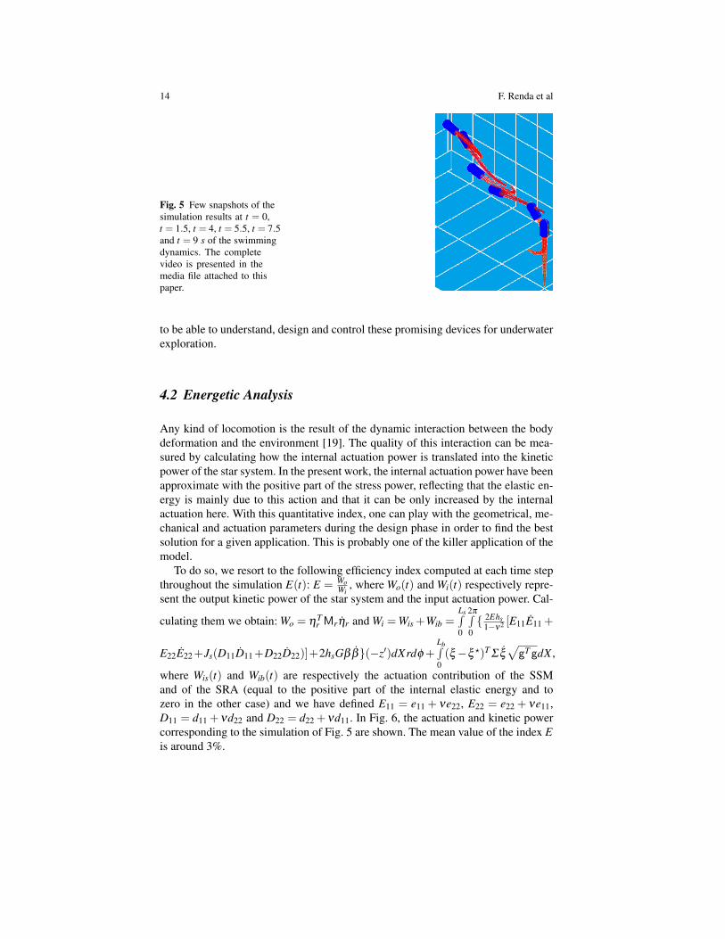
Although a simple actuation pattern has been applied, a complex swimmingdynamics came out from the fluid-structure interaction, with unexpected turningaround the symmetry axis of the shell mantle (e3) due to a torsional torque occurredduring the switching from one bending to the other. This represents a further moti-vation toward the development of a proper model of the SUUVs dynamics, in order

14 F. Renda et al

Fig. 5 Few snapshots of thesimulation results at t = 0,t = 1.5, t = 4, t = 5.5, t = 7.5and t = 9 s of the swimmingdynamics. The completevideo is presented in themedia file attached to thispaper.

to be able to understand, design and control these promising devices for underwaterexploration.

4.2 Energetic Analysis

Any kind of locomotion is the result of the dynamic interaction between the bodydeformation and the environment [19]. The quality of this interaction can be mea-sured by calculating how the internal actuation power is translated into the kineticpower of the star system. In the present work, the internal actuation power have beenapproximate with the positive part of the stress power, reflecting that the elastic en-ergy is mainly due to this action and that it can be only increased by the internalactuation here. With this quantitative index, one can play with the geometrical, me-chanical and actuation parameters during the design phase in order to find the bestsolution for a given application. This is probably one of the killer application of themodel.

To do so, we resort to the following efficiency index computed at each time stepthroughout the simulation E(t): E = Wo

Wi, where Wo(t) and Wi(t) respectively repre-

sent the output kinetic power of the star system and the input actuation power. Cal-

culating them we obtain: Wo = ηTr Mrηr and Wi =Wis +Wib =

Ls∫0

2π∫0 2Ehs

1−ν2 [E11E11 +

E22E22+Js(D11D11+D22D22)]+2hsGββ(−z′)dXrdφ +Lb∫0(ξ−ξ ?)T Σξ

√gTgdX ,

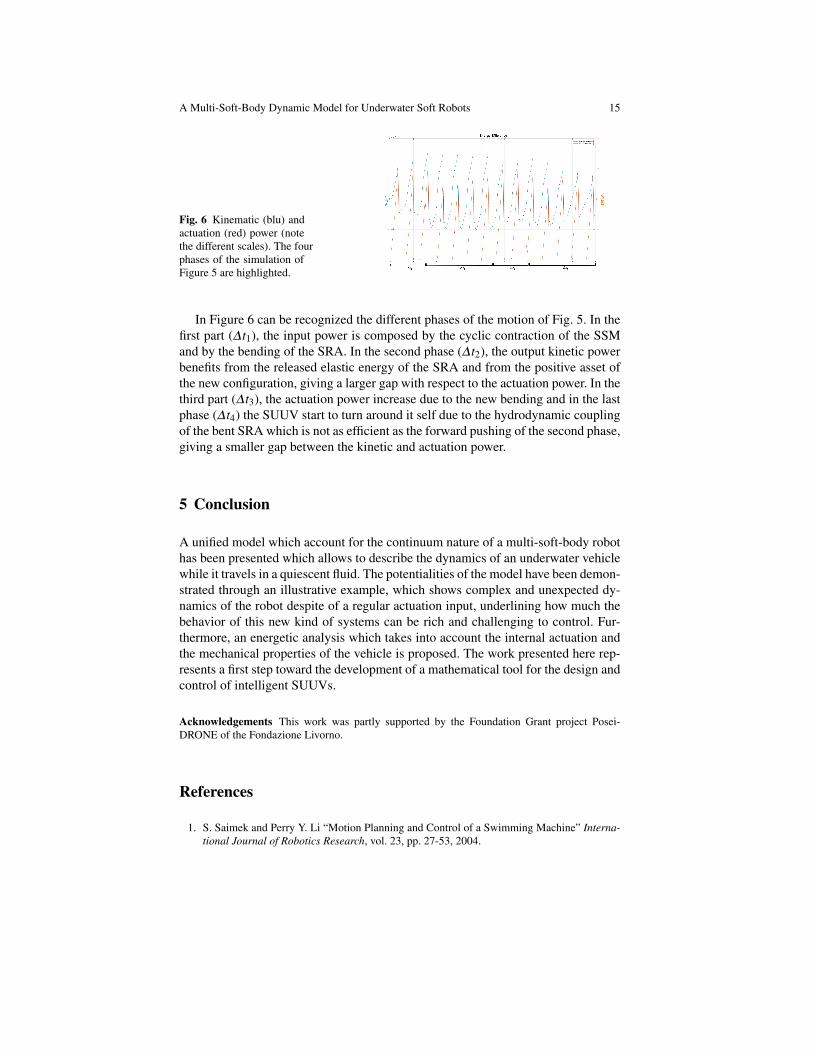
where Wis(t) and Wib(t) are respectively the actuation contribution of the SSMand of the SRA (equal to the positive part of the internal elastic energy and tozero in the other case) and we have defined E11 = e11 + νe22, E22 = e22 + νe11,D11 = d11 +νd22 and D22 = d22 +νd11. In Fig. 6, the actuation and kinetic powercorresponding to the simulation of Fig. 5 are shown. The mean value of the index Eis around 3%.

A Multi-Soft-Body Dynamic Model for Underwater Soft Robots 15

Fig. 6 Kinematic (blu) andactuation (red) power (notethe different scales). The fourphases of the simulation ofFigure 5 are highlighted.

In Figure 6 can be recognized the different phases of the motion of Fig. 5. In thefirst part (∆ t1), the input power is composed by the cyclic contraction of the SSMand by the bending of the SRA. In the second phase (∆ t2), the output kinetic powerbenefits from the released elastic energy of the SRA and from the positive asset ofthe new configuration, giving a larger gap with respect to the actuation power. In thethird part (∆ t3), the actuation power increase due to the new bending and in the lastphase (∆ t4) the SUUV start to turn around it self due to the hydrodynamic couplingof the bent SRA which is not as efficient as the forward pushing of the second phase,giving a smaller gap between the kinetic and actuation power.

5 Conclusion

A unified model which account for the continuum nature of a multi-soft-body robothas been presented which allows to describe the dynamics of an underwater vehiclewhile it travels in a quiescent fluid. The potentialities of the model have been demon-strated through an illustrative example, which shows complex and unexpected dy-namics of the robot despite of a regular actuation input, underlining how much thebehavior of this new kind of systems can be rich and challenging to control. Fur-thermore, an energetic analysis which takes into account the internal actuation andthe mechanical properties of the vehicle is proposed. The work presented here rep-resents a first step toward the development of a mathematical tool for the design andcontrol of intelligent SUUVs.

Acknowledgements This work was partly supported by the Foundation Grant project Posei-DRONE of the Fondazione Livorno.

References

1. S. Saimek and Perry Y. Li “Motion Planning and Control of a Swimming Machine” Interna-tional Journal of Robotics Research, vol. 23, pp. 27-53, 2004.

16 F. Renda et al

2. J. E. Colgate and K. M. Lynch “Mechanics and control of swimming: a review” IEEE Journalof Oceanic Engineering, vol. 29, pp. 660-673, 2004.

3. A. D. Marchese, C. D. Onal and D. Rus “Autonomous Soft Robotic Fish Capable of EscapeManeuvers Using Fluidic Elastomer Actuators” Soft Robotics, vol. 1, pp. 75-87, 2014.

4. B.A. Trimmer “Soft Robots” Current Biology, vol. 23, pp. 639-641, 2013.5. A. Arienti, M. Calisti, F. Giorgio-Serchi and C. Laschi “PoseiDRONE: design of a soft-bodied

ROV with crawling, swimming and manipulation ability” Proceedings of the MTS/IEEEOCEANS conference, San Diego, CA, USA, September, 21-27, 2013.

6. F. Giorgio-Serchi, A. Arienti, I. Baldoli and C. Laschi “An elastic pulsed-jet thruster for SoftUnmanned Underwater Vehicles” Robotics and Automation (ICRA), 2013 IEEE InternationalConference on, pp.5103,5110, 6-10 May 2013.

7. F. Giorgio-Serchi, A. Arienti and C. Laschi “A soft unamnned underwater vehicle with aug-mented thrust capability” Proceedings of the MTS/IEEE OCEANS conference, San Diego,CA, USA, September, 21-27, 2103.

8. F. Renda, M. Giorelli, M. Calisti, M. Cianchetti, C. Laschi, ”Dynamic Model of a Multibend-ing Soft Robot Arm Driven by Cables” Robotics, IEEE Transactions on, Vol 30, no 5, pp.1109-1122, 2014.

9. M. Calisti, M. Giorelli, G. Levy, B. Mazzolai, B. Hochner, C. Laschi and P. Dario “Anoctopus-bioinspired solution to movement and manipulation for soft robots” Bioinspirationand Biomimetics, vol. 6, pp. 1-10, 2011.

10. M. Giorelli, F. Giorgio-Serchi, A. Arienti and C. Laschi “Forward speed control of a pulsed-jet soft-bodied underwater vehicle” Proceedings of the MTS/IEEE OCEANS conference, SanDiego, CA, USA, September, 21-27, 2013.

11. J. C. Simo “A finite strain beam formulation. The three dimensional dynamic problem: partI” Comput. Methods Appl. Mech. Eng., vol. 49, pp. 55-70, 1985.

12. J. C. Simo and D. D. Fox, ”On stress resultant geometrically exact shell model. Part I: formu-lation and optimal parametrization” Journal Computer Methods in Applied Mechanics andEngineering vol. 72, no. 3, pp. 267-304, Mar 1989.

13. F. Renda, F. Giorgio-Serchi, F. Boyer and C. Laschi ”Structural Dynamics of a Pulsed-JetPropulsion System for Underwater Soft Robots” Int J Adv Robot Syst, vol. 12, no. 68, 2015.

14. F. Renda, F. Giorgio-Serchi, F. Boyer and C. Laschi ”Locomotion and Elastodynamics Modelof an Underwater Shell-like Soft Robot” Robotics and Automation (ICRA), 2015 IEEE Inter-national Conference on, pp.1158,1165, 26-30 May 2015, Seattle, USA, May 26-30, 2015.

15. F. Giorgio-Serchi, F. Renda, M. Calisti and C. Laschi, ”Thrust depletion at high pulsationfrequencies in underactuated, soft-bodied, pulsed-jet vehicles ”, MTS/IEEE OCEANS, Genoa,Italy, May 19-21, 2015.

16. S. S. Antman, Nonlinear Problems of Elasticity, 2nd edn (Applied Mathematical Sciences vol107) (New York:Springer), 2005.

17. F. Boyer, M. Porez and W. Khalil “Macro-Continuous Computed Torque Algorithm for aThree-Dimensional Eel-Like Robot” Robotics, IEEE Transactions on, vol. 22, no.4, pp. 763775, 2006.

18. F. Boyer, S. Ali and M. Porez “Macrocontinuous Dynamics for Hyperredundant Robots: Ap-plication to Kinematic Locomotion Bioinspired by Elongated Body Animals” Robotics, IEEETransactions on , vol. 28, no.2, pp. 303 317, April 2012.

19. F. Boyer and A. Belkhiri “Reduced locomotion dynamics with passive internal DoF: appli-cation to nonholonomic and soft robotics” Robotics, IEEE Transactions on, vol.30, no.3,pp.578,592, June 2014.