A Multi-scale Modeling System: Developments, Applications and Critical Issues

Wei-Kuo Tao1, Jiundar Chern1,2, Robert Atlas3, David Randall4, Xin Lin2,6, Marat Khairoutdinov4, Jui-Lin Li5, Duane E. Waliser5, Arthur Hou6,

Christa Peters-Lidard7, William Lau1, and Joanne Simpson1

1Laboratory for Atmospheres

NASA/Goddard Space Flight Center Greenbelt, MD 20771, USA

2Goddard Earth Sciences and Technology Center

University of Maryland, Baltimore County Baltimore, MD

3NOAA Atlantic Oceanographic and Meteorological Laboratory

Miami FL 33149

4Department of Atmospheric Science Colorado State University Fort Collins, CO 80523

5 NASA/Jet Propulsion Laboratory-California Inst. of Technology

Pasadena, CA 91109

6Goddard Modeling Assimilation Office Greenbelt, MD 20771

7Hydrological Sciences Branch

Greenbelt, MD 20771

February 5, 2007

J. Geophy. Res.

----- 1 Corresponding author address: Dr. Wei-Kuo Tao, Code 613.1, NASA Goddard Space Flight Center, Greenbelt, MD 20771, tao@agnes.gsfc.nasa.gov

Abstract

A multi-scale modeling framework (MMF), which replaces the conventional cloud

parameterizations with a cloud-resolving model (CRM) in each grid column of a GCM,

constitutes a new and promising approach. The MMF can provide for global coverage and

two-way interactions between the CRMs and their parent GCM. The GCM allows global

coverage and the CRM allows explicit simulation of cloud processes and their interactions

with radiation and surface processes.

A new MMF has been developed that is based the Goddard finite volume GCM

(fvGCM) and the Goddard Cumulus Ensemble (GCE) model. This Goddard MMF produces

many features that are similar to another MMF that was developed at Colorado State

University (CSU), such as an improved surface precipitation pattern, better cloudiness,

improved diurnal variability over both oceans and continents, and a stronger, propagating

Madden-Julian oscillation (MJO) compared to their parent GCMs using conventional cloud

parameterizations. Both MMFs also produce a precipitation bias in the western Pacific

during Northern Hemisphere summer. However, there are also notable differences between

two MMFs. For example, the CSU MMF simulates less rainfall over land than its parent

GCM. This is why the CSU MMF simulated less overall global rainfall than its parent GCM.

The Goddard MMF overestimates global rainfall because of its oceanic component. Some

critical issues associated with the Goddard MMF are presented in this paper.

1. Introduction

The foremost challenge in parameterizing convective clouds and cloud systems in large-scale

models are the many coupled, dynamical and physical processes that interact over a wide

range of scales, from microphysical scales to the synoptic and planetary scales. This makes

the comprehension and representation of convective clouds and cloud systems one of the

most complex scientific problems in earth science. During the past decade, the GEWEX

Cloud System Study (GCSS) has pioneered the use of single-column models (SCMs) and

cloud-resolving models (CRMs; also called cloud-system resolving models or CSRMs) for

the evaluation of the cloud and radiation parameterizations in general circulation models

(GCMs; e.g., GCSS 1993). These activities have uncovered many systematic biases in the

radiation and cloud parameterizations of GCMs and have lead to the development of new

schemes (e.g., Pincus et al. 2003; Zhang 2002). Comparisons between SCMs and CRMs

using the same large-scale forcing derived from field campaigns have demonstrated that

CRMs are superior to SCMs in the prediction of temperature and moisture tendencies (e.g.,

Das et al. 1999, Randall et al. 2003a, Xie et al. 2005). This result suggests that CRMs can

be important tools for improving the representation of moist processes in GCMs.

At present, however, CRMs are not global models and can only simulate clouds and

cloud systems over relatively small domains. In GCSS-style tests, the CRM results depend

strongly on the quality of the input large-scale forcing, and it is difficult to separate model

errors from observational forcing errors. Furthermore, offline CRM simulations with

observed forcing allow only one-way interaction (large-scale to cloud-scale) and cannot

simulate the effects of cloud and radiation feedbacks on the large-scale circulation. Recently

Grabowski and Smolarkiewicz (1999) and Khairoutdinov and Randall (2001) proposed a

multi-scale modeling framework (MMF, sometimes termed a “super-parameterization”),

which replaces the conventional cloud parameterizations with a CRM in each grid column of

a GCM. The MMF can explicitly simulate deep convection, cloudiness and cloud overlap,

cloud-radiation interaction, surface fluxes, and surface hydrology at the resolution of a CRM.

It has global coverage, and allows two-way interactions between the CRMs and a GCM. An

overview of this promising approach is given in Randall et al. (2003b) and Khairoutdinov et

al. (2005). An MMF can be considered as a natural extension of the current SCM and CRM

modeling activities of GCSS, NASA’s Modeling Analyses and Modeling (MAP) program,

the U.S. Department of Energy’s Atmospheric Radiation Measurements (ARM) Program,

and other programs devoted to improving cloud parameterizations in GCMs.

This paper describes the main characteristics of a new MMF developed at the

Goddard Space Flight Center. The performance and applications of the Goddard MMF are

analyzed for two different climate events, the 1998 El Nino and the 1999 La Nina. The

differences and similarities between the Colorado State University (CSU) MMF

(Khairoutdinov et al. 2005) and the Goddard MMF are summarized. Results from the

Goddard MMF are compared with those from a GCM using conventional cloud

parameterizations. In addition, some critical issues associated with the Goddard MMF are

discussed.

2. Multi-scale Modeling System

The Goddard MMF is based the NASA Goddard finite-volume GCM (fvGCM) and the

Goddard Cumulus Ensemble model (GCE, a CRM). The fvGCM provides global coverage

while the GCE allows for the explicit simulation of cloud processes and their interactions

with radiation and surface processes. This coupled modeling system allows cloud processes

to be simulated on a variety of scales. The main characteristics of the fvGCM, GCE and

Goddard MMF are briefly summarized in this section.

2.1 fvGCM

The fvGCM has been constructed by combining the finite-volume dynamic core developed at

Goddard (Lin 2004) with the physics package of the NCAR Community Climate Model

CCM3, which represents a well-balanced set of processes with a long history of development

and documentation (Kiehl et al. 1998). The unique features of the finite-volume dynamical

core include: an accurate conservative flux-form semi-Lagrangian transport algorithm

(FFSL) with a monotonicity constraint on sub-grid distributions that is free of Gibbs

oscillation (Lin and Rood 1996, 1997), a terrain-following Lagrangian control-volume

vertical coordinate, a physically consistent integration of the pressure gradient force for a

terrain-following coordinate (Lin 1997), and a mass-, momentum-, and total-energy-

conserving vertical remapping algorithm. The physical parameterizations of the fvGCM

have been upgraded by incorporating the gravity-wave drag scheme of the NCAR Whole

Atmosphere Community Model (WACCM) and the Community Land Model version 2

(CLM-2; Bonan et al. 2002). This model has been applied in climate simulation, data

assimilation and prediction modes (Atlas et al. 2005, Shen et al. 2006a,b). Depending upon

the application, the number of levels varies between 32 and 64, while the horizontal grid

spacing varies between 2.5o and 0.125o.

2.2 GCE model

The GCE model has been developed and improved at Goddard Space Flight Center over the

past two decades. The development and main features of the GCE were published in Tao

and Simpson (1993) and Tao et al. (2003). A review of the applications of the GCE to

developing a better understanding of precipitation processes can be found in Simpson and

Tao (1993) and Tao (2003). The 3D version of the GCE is typically run using 256 x 256 up

to 1024 x 1024 horizontal grid points at 1-2 km resolution or better.

A Kessler-type two-category liquid water (cloud water and rain) microphysical

formulation is used with a choice of two three-class ice formulations (3ICE), namely that of

Lin et al. (1983) and the Lin scheme modified to adopt slower graupel fall speeds as reported

by Rutledge and Hobbs (1984). The sedimentation of falling ice crystals was recently

included in the GCE scheme based on Heymsfield and Donner (1990) and Heymsfield and

Iaquinta (2000), as discussed in detail in Hong et al. (2004). Two detailed, spectral-bin

models (Khain et al. 1999, 2000; Chen and Lamb 1999) have also been implemented into the

GCE. Atmospheric aerosols are included using number density size-distribution functions.

The explicit spectral-bin microphysics can be used to study cloud-aerosol interactions and

nucleation scavenging of aerosols as well as the impact of different concentrations and size

distributions of aerosol particles upon cloud formation (Fan et al. 2006; Li et al. 2006).

These new microphysical schemes require the multi-dimensional Positive Definite Advection

Transport Algorithm (MPDATA, Smolarkiewicz and Grabowski 1990) to avoid

"decoupling" between mass and number concentration. Solar and infrared radiative transfer

processes and their explicit interactions with clouds and the generation of subgrid-scale

kinetic energy for both dry and moist processes are considered.

A sophisticated land surface modeling software package known as the Land

Information System (LIS; Kumar et al. 2006) has recently been coupled with the GCE. LIS

consists of an ensemble of land surface models (LSMs), including the Community Land

Model, (CLM; Bonan et al. 2002); the community Noah LSM (Noah; Ek et al. 2003), and

the Variable Infiltration Capacity model (VIC; Liang et al. 1996), among others. LIS is

capable of being run in two modes: (i) fully coupled or “forecast” mode, where all

meteorological inputs come from an atmospheric model such as GCE or WRF and (ii)

uncoupled or “analysis” mode, where all meteorological inputs come from a combination of

atmospheric analyses, satellite data and in situ station data. Because LIS can execute at

horizontal spatial resolutions as fine as tens of meters--given that appropriate topography,

soils, land cover and vegetation data is available--it is capable of resolving mesoscale

features, including urban areas, lakes, and agricultural fields. This capability means that the

impact and scaling of such heterogeneity on coupled cloud modeling can be studied. High-

resolution GCE-LIS simulations (Zeng et al. 2006) indicate that the land surface can have an

impact on cloud and precipitation processes especially for less-organized convective clouds.

2.3 A Coupled fvGCM-GCE Modeling System

A prototype MMF has been developed at Goddard based on the fvGCM and 2D GCE. It

includes the fvGCM run with 2.5o x 2o horizontal grid spacing with 32 layers from the

surface to 0.4 hpa, and the 2D (x-z) GCE using 64 horizontal grids (in the east-west

orientation) and 32 levels with 4 km horizontal grid spacing and cyclic lateral boundaries.

The time step for the 2D GCE is 10 seconds, and the fvGCM-GCE coupling interval is one

hour (which is the fvGCM physical time step) at this resolution.

Because the vertical coordinate of the fvGCM (a terrain-following coordinate) is

different from that of the GCE (a z coordinate), vertical interpolations are needed in the

coupling interface. To interpolate fields from the GCE to the fvGCM, an existing fvGCM

finite-volume piecewise parabolic mapping (PPM) algorithm is used, which conserves the

mass, momentum, and total energy. A new finite-volume PPM algorithm, which conserves

mass, momentum and moist static energy in the z coordinate is being developed to

interpolate fields from the fvGCM to the GCE.

Table 1 compares the main characteristics of the Goddard and CSU MMFs. More

CRMs, more frequent updating of the radiative processes (i.e., every 3 minutes), and inline

cloud statistics (every minute) in the Goddard MMF, all increase the computational

requirements compared to the CSU MMF.

3. Results

3.1 Performance of the Goddard MMF

The Goddard MMF has been evaluated against observations at inter-annual, intra-seasonal,

and diurnal time scales under two different climate scenarios, namely, the 1998 El Nino and

the 1999 La Nina. The model was forced by the observed sea surface temperatures (SSTs),

and the initial conditions came from the Goddard Earth Observing System Version-4

(GEOS-4, Bloom et al. 2005) re-analyses at 0000 UTC 1 November 1997 and 1998,

respectively. Similar runs with the same initial conditions and SSTs were performed using

the fvGCM with NCAR CCM3 physics. The moist parameterization in the fvGCM includes

the Zhang and MacFarlane (1995) scheme for deep convection and the Hack (1994) scheme

for shallow and middle-level convection processes. The cloud parameterization follows a

simple diagnosed condensation parameterization, and the cloud fraction is diagnosed

following Slingo (1987). Both models have the same horizontal and vertical resolution (2o

by 2.5o in the horizontal and 32 layers in the vertical).

Figure 1 shows the geographical distribution of simulated precipitation for January

and July 1998 from the MMF and fvGCM, along with the corresponding observations from

the Tropical Rainfall Measurement Mission (TRMM, Simpson et al. 1988, 1996) Microwave

Imager (TMI, Kummerow et al. 2001). In general, given the observed SST forcing, the

observed patterns of monthly-mean precipitation can be realistically simulated by both the

MMF and fvGCM for extra-tropical storm tracks and the Tropics. The shift in tropical

precipitation to the central Pacific in January 1998 during the El Nino is well captured. The

Inter-Tropical Convergence Zone (ITCZ), the South Pacific Convergence Zone (SPCZ), and

the South Atlantic Convergence Zone (SACZ) are also well reproduced. The MMF

precipitation patterns and dry areas tend to be slightly more realistic than those of the

fvGCM; in particular, the unrealistic double ITCZ simulated by the fvGCM for July 1998 is

not present in the MMF.

There are apparent biases in the MMF however: monthly-mean precipitation

averaged over the Tropics is about 30% (4-6%) more than the TRMM observations (fvGCM)

in both winter and summer. The MMF precipitation in the western Pacific, eastern tropical

Pacific, Bay of Bengal and western India Ocean is too active during summer; a similar

phenomenon occurs in simulations with the CSU MMF and has been called the “Great Red

Spot” by Khairoutdinov et al. (2005). It is remarkable that both MMFs exhibit the Great

Red Spot problem despite the many differences in their GCM dynamical cores, CRM

dynamics, microphysics parameterizations, radiation, turbulence, and coupling strategies

(Table 1). Due to the nonlinear coupling between the GCM and the CRM, the physical

cause(s) of the Great Red Spot is(are) very difficult to isolate and identify. The use of 2D

CRMs with cyclic lateral boundary conditions, which do not allow deep convective systems

to propagate to the neighboring GCM grid boxes, is believed to be one of the causes of the

Great Red Spot (Khairoutdinov et al. 2005). The cyclic lateral boundary conditions could

lead to an excessive local convective-wind-evaporation feedback and ultimately the Great

Red Spot (Luo and Stephens 2006). However, Khairoutdinov et al. (2005) have

demonstrated that the Great Red Spot can be eliminated with a 3D CRM (using a small

domain, 8 x 8 grid points), especially when convective momentum transport is included1.

Their study suggests that dimensionality (2D vs 3D CRM) and sampling in one direction

might be the cause of the Great Red Spot.

Vertical velocities simulated by the Goddard MMF are stronger, particularly over the

Great Red Spot region, than those in the fvGCM. This may be another factor in producing

the Great Red Spot and could also explain why there is more precipitation in the MMF than

fvGCM. Furthermore, the compensating downward motion (through mass conservation) was

also stronger and produced stronger warming and drying in the MMF. This could cause the

MMF to simulate larger and more realistic non-raining regions.

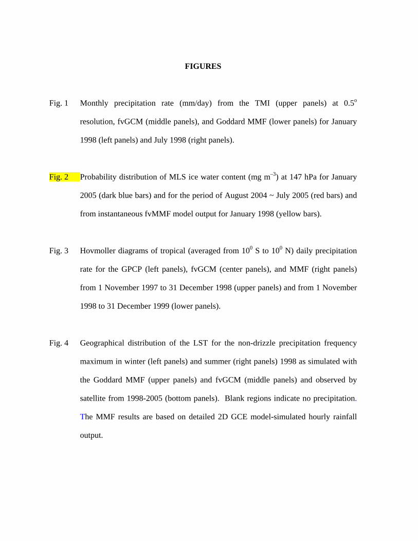
Figure 2 shows probability distribution functions (PDFs) of ice water content (IWC)

at 147 hPa based on Microwave Limb Sounder (MLS) retrievals for January 2005 and for the

period August 2004 to July 2005 as well as hourly instantaneous values of IWC from the

Goddard MMF for January 1998. The MLS-retrieved annual (red color bars) and January

(dark blue color bars) PDFs are similar, implying that the PDF is not too sensitive to the time

of year when the whole Tropics is considered. Moreover, the PDFs clearly illustrate the

sensitivity limits of the MLS instrument, namely that the precision of the MLS retrievals

dictate a lower limit on the IWC values that can be detected, roughly ~0.4 (mg m-3) at this

pressure level. The Goddard MMF values, on the other hand, exhibit nonzero values in this

low IWC range (< 0.4 mg m-3). In addition, the Goddard MMF has a lower percentage of

1 Their results also showed that precipitation amount was very sensitive to convective momentum transport when the 3D CRM was used. One the other hand, the precipitation amount is

IWCs between 1 ~ 20 (mg m-3) than does the MLS data. The large ICW range (> 25.0 mg m-

3) simulated by the Goddard MMF occurs mainly over continents or coasts except for in the

central and eastern Pacific during January 1998. Large vertical cloud velocities associated

with storms that developed over land and coastal areas may explain the larger IWCs

[convective available potential energy (CAPE) is larger over land than ocean]. For January

1998, deep convective systems responding to the warm SSTs in the central and eastern

Pacific could produce large amounts of ice aloft. Overall, the comparison between the

Goddard MMF and MLS IWC values generally shows good agreement in terms of the shape

of the distribution. Similar results can be found for July 1998 and January and July 1999

(not shown).

The Madden-Julian Oscillation (MJO, Madden and Julian 1972, 1994), also known as

the 30-60 day wave, is one of the most prominent large-scale features of the tropical general

circulation. While the MJO is evident in circulation fields throughout the Tropics (Madden

and Julian 1972; Knutson and Weickmann 1987), it is typically characterized by deep

convection originating over the Indian Ocean and subsequent eastward propagation into the

Pacific Ocean. Figure 3 shows Hovmoller diagrams of the daily tropical precipitation rate

averaged between 10ºS and 10ºN from the Global Precipitation Climatology Project (GPCP),

the fvGCM and Goddard MMF for 1998 and 1999. Both the fvGCM and MMF realistically

reproduce the El Nino-associated eastward shift in the broad envelope of convection from the

western Pacific warm pool to the eastern Pacific during winter 1997 and spring 1998 and the

westward shift after summer 1998. During the 1999 La Nina, the broad-scale deep

quite similar in the Goddard MMF with and without convective momentum transport.

convective rain remains over the western Pacific warm pool region. Overall, the MMF

(fvGCM) tends to produce stronger (weaker) convection than observed. Superimposed on

the broad inter-annual patterns, the MMF shows vigorous convection propagating eastward

at 30-60-day time scales, similar to what is observed. In contrast, the fvGCM run only

shows some westward-propagating convection signals; the eastward-propagating MJO

signals are virtually nonexistent. These results are consistent with the earlier findings (e.g.,

Randall et al. 2003b; Grabowski 2003, 2004) that MMFs can more realistically simulate the

tropical intra-seasonal oscillation than GCMs with conventional cloud parameterizations.

The diurnal cycle is a fundamental mode of atmospheric variability. Successful

simulation of the diurnal variability of the hydrologic cycle and radiative energy budget

provides a robust test of physical processes represented in atmospheric models (e.g., Slingo

et al. 1987; Randall et al. 1991; Lin et al. 2000). Figure 4 shows the geographical

distribution of the local solar time (LST) of the non-drizzle precipitation frequency

maximum in winter (left panels) and summer (right panels) of 1998 as simulated by the

Goddard MMF (top panels) and the fvGCM (middle panels). Satellite microwave rainfall

retrievals from a 5-satellite constellation including the TRMM TMI, Special Sensor

Microwave Imager (SSMI) from the Defense Meteorological Satellite Program (DMSP)

F13, F14 and F15, and the Advanced Microwave Scanning Radiometer – Earth Observing

System (AMSR-E) onboard the Aqua satellite are analyzed at 1-h intervals from 1998 to

2005 for comparison. The non-drizzle precipitation is defined as precipitation that occurs

such that the 1-h averaged rain rate is larger than 1 mm/day (see Lin et al. 2006).

Satellite microwave rainfall retrievals in general show that precipitation occurs most

frequently in the afternoon to early evening over the major continents such as South and

North America, Australia, and west and central Europe, reflecting the dominant role played

by direct solar heating of the land surface. Over open oceans, a predominant early morning

maximum in rain frequency can be seen in satellite observations, consistent with earlier

studies (see a review by Sui et al. 1997, 2006). The MMF is superior to the fvGCM in

reproducing the correct timing of the late afternoon and early evening precipitation

maximum over land and the early morning precipitation maximum over the oceans. The

fvGCM, in contrast, produces a dominant morning maximum rain frequency over major

continents. Additional and more detailed comparisons between the observed and MMF-

simulated diurnal variation of radiation fluxes, clouds and precipitation under different large-

scale weather patterns and different climate regimes will be published elsewhere.

3.2 Comparison of the Goddard and CSU MMFs

Despite differences in model dynamics, coupling interfaces and physics between the

Goddard and CSU MMFs, both simulate more realistic and stronger MJOs than traditional

GCMs. However, both MMFs also have similar model biases, such as the Great Red Spot

problem and the over-prediction of total surface rainfall over ocean compared to observations

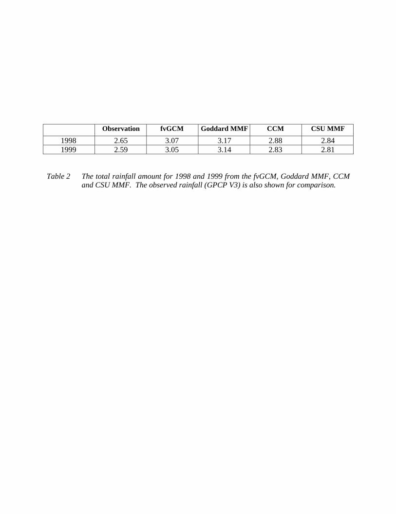
and the parent GCM (Tables 2 and 3). All of the model runs (i.e., from the two GCMs and

the two MMFs) overestimate global rainfall compared to satellite estimates for 1998 (El

Nino) and 1999 (La Nina). However, the CCM and CSU MMF-simulated rainfall are in

better agreement with satellite estimates than the fvGCM and Goddard MMF for both years.

All of the model runs show less variation in total rainfall compared to satellite estimates. It

might be expected that the MMF-simulated rainfall would be close to that of its parent GCM

because many of the physical processes (i.e., surface processes, radiation, and SST) in the

MMF are still the same as in the GCM. In addition, the key coupling strategy or design of

the MMF is not to allow the MMF’s mean field to systematically “drift” away from the

corresponding GCM fields. One interesting result is that the Goddard MMF simulated more

rainfall (about 3%) than its parent GCM for both years. In contrast, the CSU MMF

simulated less rainfall (about 1%) than its parent GCM.

Both MMFs overestimate oceanic rainfall (2-3%) compared to their parent GCMs

and satellite estimates for both years (Table 3). The CSU MMF simulated less rainfall over

land than its parent GCM. This is why the CSU MMF simulated less global rainfall than its

parent GCM (Table 2). The Goddard MMF overestimates global rainfall because of its

oceanic component. The CSU MMF simulated the same amount of oceanic rainfall in both

1998 and 1999, implying that the CSU MMF is more sensitive to its land processes than its

oceanic processes. The Goddard MMF shows slightly more variation in rainfall over ocean

than land between 1998 and 1999.

Since all of the models (i.e., fvGCM, CCM, Goddard and CSU MMFs) and the

satellite observations show almost identical global high, middle and low cloud amounts for

1998 and 1999, only the cloud amounts for 1998 are shown in Table 4. Both of the MMFs

exhibit much better agreement with International Satellite Cloud Climatology Project

(ISCCP) cloud amounts (especially high and low) than do the GCMs. The CSU MMF-

simulated high cloud amount agrees best with the satellite estimate.

The MMF approach is extremely computer intensive and can produce immense data

sets. In this paper, only the variables and features inherent in their parent GCMs are

compared. A more detailed comparison between the two MMFs for longer simulations (i.e.,

5-10 year integrations), including simulated cloud properties from their CRM components as

well as their improvements and sensitivities (see section 4), will be conducted in a separate

paper.

4. Issues and Future Research

Despite the apparent promise of the MMF, only limited long-term simulations have been

carried out with the system due to computational resources. To fully understand the

strengths and weakness of the MMF approach in climate modeling, more research is needed

to systematically study these issues with either the MMF itself or with offline CRM

simulations. The model results also need to be tested thoroughly and rigorously against

satellite and ground-based observations.

In addition, there are still many critical issues related to the MMF that may have a

major impact on MMF performance. Specifically, the configuration of the CRMs within the

MMF and the assumptions/physics used in the CRMs need to be addressed.

4.1 Configuration of CRMs within the MMF

Current MMF studies have only used 2D CRMs with cyclic lateral boundary conditions

as proposed by Grabowski and Smolarkiewicz (1999) and Grabowski (2001). The

potential weaknesses of the current framework are: (1) use of cyclic lateral boundary

conditions in the CRM, (2) CRMs in neighboring GCM grid boxes can communicate

only through the GCM, (3) the use of simple approaches for communication between the

GCM and the CRMs, (4) use of coarse vertical and horizontal grid sizes in the CRM (4

km for the latter in the present study), (5) the absence of land surface and terrain effects

in the CRMs, (6) the two-dimensionality of the CRMs, (7) each CRM converges to a 1D

cloud model as the GCM grid size approaches that of the CRM, (8) the use of one single

type of bulk microphysics (i.e., a 3ice scheme with graupel as the third class of ice) and

parameterizations for radiation and sub-grid-scale turbulent processes in the CRM, and

(9) momentum feedbacks/interactions between the CRMs and GCM are not accounted

for. Problems (1)-(3) have been recognized and studied by Grabowski (2001, 2004) and

Jung and Arakawa (2005). Khairoutdinov and Randall (2001) tested the sensitivity of the

CRM results to the domain geometry and horizontal grid size using an offline 2D CRM.

Problems (6) and (7) could be addressed by the quasi-3D approach (Randall et al. 2003b;

Arakawa 2004; see Fig. 5b). However, the quasi-3D approach is more difficult to

implement and more expensive computationally. At Goddard, an MMF based on a

global 2D CRM (see Fig. 5a) is also being developed to address issues (2) and (7). In

addition to thermodynamic feedback, dynamic (momentum forcing) feedback is also

needed.

4.2 Issues related to the CRM used in the MMF

Some of the deficiencies in the current MMF are related to the dynamic and physical

processes used in the CRM. These issues can be studied either by using the MMF itself or

through the use of offline 2D and/or 3D CRMs.

4.2.1 Dimensionality (2D vs 3D)

Real clouds and cloud systems are 3D. Because of the limitations of computer resources, a

2D CRM is being used in the MMF. Previous modeling studies indicated that (e.g., Tao and

Soong 1986; Lipps and Hemler 1986; Tao et al. 1987) the collective thermodynamic

feedback effect and the vertical transports of mass, sensible heat, and moisture were quite

similar between 2D and 3D numerical simulations. The fractional cloud coverage between

the 2D and 3D simulations, however, differed between 2% (in the lower troposphere) and

10% (between 300 and 400 mb) in the cases studied. In these 3D simulations, the model

domain was small and integration times were between 3 and 6 hours. However, Grabowski

et al. (1998) found that cloud statistics as well as surface precipitation were significantly

different for their 2D and 3D simulations if cloud radiation was fully interactive over their 7-

day integrations. Zeng et al. (2006) found that the 3D-simulated surface rainfall is in better

agreement with observations than its 2D for two ARM cases. They also found that the

momentum field is quite similar between 2D and 3D simulations when both models are

nudged with the same large-scale observed winds at 1, 6, 12 and 24 hour model integration

times.

Only thermodynamic feedback is allowed in the current Goddard and CSU MMFs,

although Khairoutdinov et al. (2005) did perform some tests using a 3D CRM with

momentum feedback. The 2D CRM orientation in the Goddard MMF is east-west. The CSU

MMF has been run with both east-west and north-south orientations, and the north-south

orientation has been adopted in a recent study (Khairoutdinov and Randall 2006). The

fractional cloudiness and mesoscale organization are mainly determined by the vertical shear

of the low-level wind. The surface fluxes also depend on the near-surface wind. Offline

tests comparing 2D CRM simulations using east-west and south-north configurations are

needed. The similarities and differences between 2D (east-west and south-north) and 3D for

both short and long-term integration and in both active and inactive convective periods need

to be identified.

4.2.2 Anelastic vs Compressible

The CRM dynamics can be either anelastic (Ogura and Phillips 1962), filtering out sound

waves, or compressible (Klemp and Wilhelmson 1978), allowing sound waves. The sound

waves are not important for thermal convection, but because of their high propagation speed,

they create severe restrictions on the time step used in numerical integrations. For this

reason, most cloud models (including those used in the Goddard and CSU MMFs) use an

anelastic system of equations in which sound waves have been filtered. One advantage of

the compressible system is its computational simplicity and flexibility. Sensitivity tests are

needed to examine the impact of compressibility on the MMF results.

4.2.3 Grid Size (Vertical and Horizontal)

For CRMs, the choice of horizontal and vertical grid spacing is an important issue and can

have a major impact on the resolved convective processes. For example, Tompkins and

Emanuel (2000) suggested that high vertical resolution (finer than 33 hPa) is needed to

simulate realistic water vapor profiles and stratiform precipitation processes. In addition,

much finer resolution is required for simulating realistic stratocumulus (Dr. Bjorn Stevens,

personal communication). A comprehensive study of the sensitivity of various cloud types

and/or systems to vertical and horizontal grid resolution is needed. The results from offline

CRM research can help to determine the grid size requirements for the CRMs used in MMFs.

4.2.4 Microphysics

Both the Goddard and CSU MMF use a single one-moment bulk microphysical scheme (e.g.,

the 3ICE scheme with graupel) for all clouds and cloud systems. Typically, graupel with its

low density and a high intercept (i.e., high number concentration) is used as the third class of

ice when simulating tropical oceanic systems. In contrast, hail has a high density, small

intercept, and fast fall speed and is used to simulate midlatitude continental systems

(McCumber et al. 1991; Tao et al. 1996). Therefore, sensitivity tests are required to examine

the impact of different bulk microphysical schemes (e.g., 3ICE with graupel, 3ICE with hail)

in the MMF. By comparing model results with observations, errors in the simulated

hydrometeor fields can be investigated, identified and documented, especially in regards to

uncertainties often associated with the cloud microphysical schemes. The effects of aerosols

should also be tested with advanced microphysical schemes (i.e., spectral bin microphysics

or a multi-moment scheme).

4.2.5 Land Surface

Interactions between the atmosphere and the land surface have considerable influence on

local, regional and global climate variability. Therefore, coupled land-atmosphere systems

that can realistically represent these interactions are critical for improving our understanding

of the atmosphere-biosphere exchanges of water, energy, and their associated feedbacks. By

coupling a high-resolution land surface modeling system (i.e., LIS) into the MMF, the

interaction between soil, vegetation, and precipitation processes can be studied. As only 2D

CRMs are being used in the MMF, how to specify the observed heterogeneities of land

characteristics in 2D (with cyclic lateral boundary conditions) could be a major issue.

Therefore, a method to allow heterogeneous surface processes (surface fluxes and/or land

characteristics) in the coupled CRM-LIS system needs to be developed. The simplest

method is a random distribution (Zeng et al. 2006). A more physical approach could use

PDF matching between observed surface fluxes (or land characteristics) and modeled surface

properties (i.e., the product of wind stress and air-land temperature/moisture differences, or

rainfall). Both methods will be tested to improve the MMF’s ability to represent these

processes and to identify the key land-atmosphere feedbacks and their impact on the local

and regional water and energy cycles.

5. Summary

The idea for the MMF, whereby conventional cloud parameterizations are replaced with

CRMs in each grid column of a GCM, was proposed by Grabowski and Smolarkiewicz

(1999). Khairoutdinov and Randall (2001) and Randall et al. (2003b) developed the first

MMF based on a GCM developed at NCAR (CAM) and a CRM at CSU. A second, more

recent MMF based on the fvGCM and the GCE has been developed. This Goddard MMF’s

performance was evaluated and compared against satellite observations, its parent GCM

(fvGCM) and the CSU MMF. The major highlights are as follows:

o The MMF-simulated surface precipitation pattern agrees with TRMM estimates,

especially in the non-rainy region. Compensating downward motion away from major

precipitation centers was stronger and produced stronger warming and drying in the MMF.

This could lead the MMF to simulate larger and more realistic non-raining regions.

o The comparison between the MMF and MLS IWCs generally shows good agreement

in terms of the shape of the distribution. However, the MLS did not detect the small

(between 0.1 – 0.4 mg/m3) and large IWCs (> 4 mg/m3) that were simulated in the MMF.

o The MMF-simulated diurnal variation of precipitation shows good agreement with

merged microwave observations. For example, the MMF-simulated frequency maximum

was in the late afternoon (1400-1800 LST) over land and in the early morning (0500-0700

LST) over the oceans. The fvGCM-simulated frequency maximum was too early for both

oceans and land.

o The MMF-simulated MJO shows vigorous eastward propagation at 30-60-day time

scales, similar to what is observed. In contrast, the fvGCM-simulated MJO is very weak and

the observed eastward-propagating MJO signals are nonexistent.

o Despite differences in model dynamics, coupling interfaces and physics between the

Goddard and CSU MMFs, they both performed better against observations than did their

parent GCMs. However, both MMFs also simulated the Great Red Spot (i.e., an over

estimation of precipitation in the western Pacific). The Great Red Spot problem could be due

to the cyclic lateral boundary conditions, the two-dimensionality of the CRMs, localized

convective-wind–evaporation feedback, stronger vertical upward motion or a combination of

factors. There are also differences between the two MMFs. For example, the CSU MMF

simulated less rainfall over land than its parent GCM. This is why the CSU MMF simulated

less global rainfall than its parent GCM. The Goddard MMF, however, overestimates global

rainfall because of its oceanic component.

o Comparisons between the two MMFs for 1998 and 1999 were based on variables

from their parent GCMs. A more detailed comparison between the two MMFs for longer

simulations (i.e., 5-10 years integration), including simulated cloud properties from their

CRM components, is needed.

o A better design for future MMFs is needed and being developed (i.e, quasi-3D and

global 2D). Since the embedded CRMs allow for the explicit simulation of cloud processes

and their interaction with radiation and surface processes, the CRM’s own dynamic and

physical processes could cause deficiencies in the current MMF. Major CRM-related issues

were discussed in detail (Section 4).

MMFs can bridge the gap between traditional CRM simulations that have been

applied over the past two decades and future non-hydrostatic high-resolution global CRMs.

The traditional CRM needs large-scale advective forcing in temperature and water vapor

from intensive sounding networks deployed during major field experiments or from large-

scale model analyses to be imposed as an external forcing (Soong and Ogura 1980; Soong

and Tao 1980; Tao and Soong 1986; Krueger et al. 1988; and many others). A weakness of

this approach is that the simulated rainfall, temperature and water vapor budget are forced to

be in good agreement with observations (see Tao 2003 for a brief review; and Randall et al.

2003a). However, there is no feedback from the CRM to the large-scale model (i.e., the

CRM environment). In contrast, an MMF allows explicit interactions between the CRM and

the GCM. Traditional CRMs can only examine the sensitivity of model grid size or physics

for one type of cloud/cloud system at a single geographic location. MMFs, however, could

be used to identify the optimal grid size and physical processes (i.e., microphysics, cloud-

radiation interaction) on a global scale.

6. Acknowledgements

The authors thank Dr. D. Anderson for his support for developing the MMF under the NASA

IDS and Cloud Modeling and Analysis Initiative (CMAI) program. The GCE is mainly

supported by the NASA Headquarters Atmospheric Dynamics and Thermodynamics

Program and TRMM. The first author and J. Simpson are grateful to Dr. R. Kakar at NASA

headquarters for his support of GCE development over the past decade. The authors also

thank Mr. S. Lang and Dr. D. Starr for proof reading and providing comments, respectively.

Acknowledgment is also made to the NASA Goddard Space Flight Center and Ames

Center for computer time used in this research.

7. References

Arakawa, A., 2004: The cumulus parameterization problem: Past, present, and future. J.

Climate, 17, 2493-2525.

Atlas, R., O. Reale, B.-W. Shen, S.-J. Lin, J.-D. Chern, W. Putman, T. Lee, K.-S. Yeh, M.

Bosilovich, and J. Radakovich, 2005: Hurricane forecasting with the high-resolution

NASA finite-volume General Circulation Model, Geophysical Research Letters, 32,

L03801, doi:10.1029/2004GL021513.

Bloom, S., A. da Silva, D. Dee, M. Bosilovich, J.-D. Chern, S. Pawson, S. Schubert, M.

Sienkiewicz, I. Stajner, W.-W. Tan, M.-L. Wu, 2005: Documentation and Validation of

the Goddard Earth Observing System (GEOS) Data Assimilation System - Version 4.

Technical Report Series on Global Modeling and Data Assimilation 104606, 26.

Bonan, G. B., K. W. Oleson, M. Vertenstein, S. Levis, X. Zeng, Y. Dai, R. E. Dickinson,

and Z.-L. Yang, 2002: The Land Surface Climatology of the Community Land Model

Coupled to the NCAR Community Climate Model. J. Clim, 15(22), 3123–3149.

Chen, J-.P., and D. Lamb, 1999: Simulation of cloud microphysical and chemical processes

using a multicomponent framework. Part II: Microphysical evolution of a wintertime

orographic cloud. J. Atmos. Sci., 56, 2293-2312.

Das, S., D. Johnson and W.-K. Tao, 1999: Single-column and cloud ensemble model

simulations of TOGA COARE convective systems, J. Meteor. Soc. Japan, 77, 803-826.

DeMott, C. A., D. A. Randall, and M. Lhairoutdinov, 2006: Convective precipitation

variability as a tool for general circulation model analysis. J. Climate, (accepted).

Ek, M. B., K. E. Mitchell, Y. Lin, E. Rogers, P. Grunmann, V. Koren, G. Gayno, and J. D.

Tarpley, 2003: Implementation of Noah land surface model advances in the National

Centers for Environmental Prediction operational mesoscale Eta model, J. Geophys. Res.,

108(D22), 8851, doi:10.1029/2002JD003296.

Fan, J., R. Zhang, G. Li, W.-K. Tao, X. Li, 2006: Simulations of cumulus clouds using a

spectral bin microphysics in a cloud resolving model. J. Geophy. Res., (in press).

GEWEX Cloud System Study (GCSS), 1993: Bull. Amer. Meteor. Soc., 74, 387-400.

Grabowski, W. W., X. Wu, and M. W. Moncrieff, and W. D. Hall, 1998: Cloud resolving

modeling of tropical cloud systems during PHASE III of GATE. Part II: Effects of

resolution and the third dimension. J. Atmos. Sci., 55, 3264-3282.

Grabowski, W. W., and P. K. Smolarkiewicz, 1999: CRCP: A cloud resolving convective

parameterization for modeling the tropical convective atmosphere. Physica, 133, 171-

178.

Grabowski, W. W., 2001: Coupling cloud processes with the large scale dynamics using the

cloud resolving convection parameterization (CRCP). J. Atmos. Sci., 58, 978-997.

Grabowski, W. W., 2003: MJO-like coherent structures: Sensitivity simulations using the

cloud-resolving convection parameterization (CRCP). J. Atmos. Sci., 60, 847-864.

Grabowski, W. W., 2004: An improved framework for superparameterization. J. Atmos. Sci.,

61, 1940-1952.

Hack, J. J., 1994: Parameterization of moist convection in the National Center for

Atmospheric Research community climate model (CCM2), J. Geophys. Res., 99 (D3),

5551-5568.

Heymsfield, A. J., and L. J. Donner, 1990: A scheme for parameterizing ice-cloud water

content in general circulation models. J. Atmos. Sci., 47, 1865-1877.

Heymsfield, A. J., and J. Iaquinta, 2000: Cirrus crystal terminal velocities. J. Atmos. Sci., 57,

916-938.

Hong, S.-Y., J. Dudhia, and S.-H. Chen, 2004: A revised approach to ice-microphysical

processes for the bulk parameterization of cloud and precipitation. Mon. Wea. Rev.,

132, 103–120.

Jung, J.-H., and A. Arakawa, 2005: Preliminary tests of multiscale modeling with a two-

dimensional framework: Sensitivity to coupling methods. Mon. Wea. Rev., 133, 649-662.

Khain, A. P., A. Pokrovsky, and I. Sednev, 1999: Some effects of cloud-aerosol interaction

on cloud microphysics structure and precipitation formation: Numerical experiments with

a spectral microphysics cloud ensemble model. Atmos. Res., 52, 195-220.

Khain, A. P., M. Ovtchinnikov, M. Pinsky, A. Pokrovsky, and H. Krugliak, 2000: Notes on

the state-of-the-art numerical modeling of cloud microphysics. Atmos. Res., 55, 159-224.

Khairoutdinov, M. F., and D. A. Randall, 2001: A cloud resolving model as a cloud

parameterization in the NCAR community climate system model: Preli-minary results.

Geophys. Res. Lett., 28, 3617-3620.

Khairoutdinov, M. F., and D. A. Randall, 2003: Cloud resolving modeling of the ARM

Summer1997 IOP: Model formulation, results, uncertainties, and sensitivities. J. Atmos.

Sci., 60, 607-625.

Khairoutdinov, M. F., D. A. Randall, and C DeMott, 2005: Simulations of the Atmospheric

General Circulation Using a Cloud-Resolving Model as a Superparameterization of

Physical Processes. J. Atmos. Sci., 62, 2136-2154.

Khairoutdinov, M. F., and D. A. Randall, 2006: Evaluation of the simulated interannual and

subseasonal variability in an AMIP-style simulation using the CSU Multiscale Modeling

Framework. J. Climate, (submitted).

Kiehl,J. T., J. J. Hack, G. B. Bonan, B. A. Boville, D. L. Williamson, and P. J. Rasch, 1998:

The National Center for Atmospheric Research Community Climate Model: CCM3. J.

Climate, 11, 1131–1150.

Klemp, J. B., and R. Wilhelmson, 1978: The simulation of three-dimensional convective

storm dynamics. J. Atmos. Sci., 35, 1070-1096.

Krueger, S.K., 1988: Numerical simulation of tropical cumulus clouds and their interaction

with the subcloud layer. J. Atmos. Sci., 45, 2221-2250.

Knutson, T. R., and K. M. Weickmann, 1987: 30-60 day atmospheric oscillations: Composite

life cycles of convection and circulation anomalies. Mon. Wea. Rev., 115, 1407-1436.

Kumar, S. V., C. D. Peters-Lidard, Y. Tian, P. R. Houser, J. Geiger, S. Olden, L. Lighty, J. L.

Eastman, B. Doty, P. Dirmeyer, J. Adams, K. Mitchell, E. F. Wood and J. Sheffield,

2006: Land Information System - An Interoperable Framework for High Resolution Land

Surface Modeling. Environmental Modeling & Software, 21, 1402-1415.

Kummerow, C., Y. Hong, W.S. Olson, S. Yang, R.F. Adler, J. McCollum, R. Ferraro, G.

Petty, D.-B. Shin, and T.T. Wilheit, 2001: The evolution of the Goddard profile

algorithm (GPROF) for rainfall estimation from passive microwave sensors. J. Appl.

Meteor., 40, 1801-1820.

Li, X., W.-K. Tao, A. Khain, J. Simpson and D. Johnson, 2006: Sensitivity of (bulk vs

explicit-bin) microphysics in cloud-resolving model simulated mid-latitude squall line:

Part I: Model validation. J. Atmos. Sci., (submitted).

Liang, X, E. F. Wood, and D. P. Lettenmaier, 1996: Surface soil moisture parameterization

of the VIC-2L model: Evaluation and modification. Global and Planetary Change. 13(1-

4), 195-206.

Lin, S.-J., 2004: A “vertically Lagrangian” finite-volume dynamical core for global models.

Mon. Wea. Rev., 32, 2293-2307.

Lin, S.-J., 1997: A finite-volume integration method for computing pressure gradient forces

in general vertical coordinates. Q. J. Roy. Met. Soc., 123, 1749-1762.

Lin, S.-J., and R. B. Rood, 1997: An explicit flux-form semi-Lagrangian shallow water

model on the sphere. Q. J. Roy. Met. Soc., 123, 2477-2498.

Lin, S.-J., and R. B. Rood, 1996: Multidimensional flux-form semi-Lagrangian transport

schemes. Mon. Wea. Rev., 124, 2046-2070.

Lin, X., D. A. Randall, and L. D. Fowler, 2000: Diurnal variability of the hydrological cycle

and radiative fluxes: Comparisons between observations and a GCM. J. Climate, 13,

4159-4179.

Lin, X., S. Zhang, and A. Y. Hou, 2006: Variational assimilation of global microwave

rainfall retrievals: Physical and dynamical impact on GEOS analyses. Conditionally Mon.

Wea. Rev., (accepted).

Lin, Y.-L., R. D. Farley, and H. D. Orville, 1983: Bulk parameterization of the snow field in

a cloud model. J. Clim.ate Appl. Meteor., 22, 1065-1092.

Lipps, F. B., and R. S. Helmer, 1986: Numerical simulation of deep tropical convection

associated with large-scale convergence. J. Atmos. Sci., 43, 1796-1816.

Luo, Z., and G. L. Stephens, 2006: An enhanced convection-wind-evaporation feedback in a

superparameterization GCM (SP-GCM) depiction of the Asian summer monsoon. J.

Geophys. Lett., 33, L06707, doi:10.1029/2005GL025060.

Madden, R. A., and P. R. Julian, 1972: Description of global-scale circulation cells in the

Tropics with a 40-50 day period. J. Atmos. Sci., 29, 1109-1123.

Madden, R. A., and P. R. Julian, 1994: Observations of the 40-50-day tropical oscillation—A

review. Mon. Wea. Rev., 122, 814-837.

McCumber, M., W.-K. Tao, J. Simpson, R. Penc, and S.-T. Soong, 1991: Comparison of ice-

phase microphysical parameterization schemes using numerical simulations of

convection. J. Appl. Meteor., 30, 987-1004.

Ogura, Y., and N. A. Phillips, 1962: Scale analysis of deep and shallow convection in the

atmosphere. J. Atmos. Sci., 19, 173-179.

Pincus, R., H. W. Baker, and J.-J. Mocrette, 2003: A fast, flexible, approximation technique

fro computing radiative transfer in inhomogeneous cloud fields. J. Geophys. Res., 108

(D13), 4376,doi:10.1029/2002JD003322.

Randall, D.A., Harshvardhan, and D.A. Dazlich, 1991: Diurnal variability of the hydrologic

cycle in a general circulation model. J. Atmos. Sci., 48, 40-62.

Randall, D., S. Krueger, C. Bretherton, J. Curry, P. Duynkerke, M. Moncrieff, B. Ryan, D.

Starr, M. Miller, W. Rossow, G. Tselioudis and B. Wielicki, 2003a: Confronting Models

with Data: The GEWEX Cloud Systems Study. Bull. Amer. Meteor. Soc., 84, 455-469.

Randall, D., M. Khairoutdinov, A. Arakawa, and W. Grabowski, 2003b: Breaking the cloud

parameteriza-tion deadlock. Bull. Amer. Meteor. Soc., 84, 1547-1564.

Rutledge, S. A., and P. V. Hobbs, 1984: The mesoscale and microscale structure and

organization of clouds and precipitation in mid-latitude clouds. Part XII: A diagnostic

modeling study of precipitation development in narrow cold frontal rainbands. J. Atmos.

Sci., 41, 2949-2972.

Shen, B.-W., R. Atlas, J.-D. Chern, O. Reale, S.-J. Lin, T. Lee, and J. Change 2006a: The

Finite Volume General Mesoscale Circulation Model: Preliminary simulations of

mesoscale vortices at 1/8 degree resolution. Geophys. Res. Lett., 33, L05801,

doi:10.1029/2005GL024594.

Shen, B.-W., R. Atlas, O. Oreale, S.-J Lin, J.-D. Chern, J. Chang, C. Henze, and J.-L. Li,

2006b: Hurricane Forecasts with a Global Mesoscale-Resolving Model: Preliminary

Results with Hurricane Katrina (2005). Geophys. Res. Lett., 2006GL026143, in press.

Simpson, J., and W.-K. Tao, 1993: The Goddard Cumulus Ensemble Model. Part II:

Applications for studying cloud precipitating processes and for NASA TRMM.

Terrestrial, Atmospheric and Oceanic Sciences (TAO), 4, 73-116.

Simpson, J., R.F. Adler, and G. North, 1988: A Proposed Tropical Rainfall Measuring

Mission (TRMM) satellite. Bull. Amer. Meteor. Soc., 69, 278-295.

Simpson, J., C. Kummerow, W.-K. Tao, and R. Adler, 1996: On the Tropical Rainfall

Measuring Mission (TRMM), Meteor. and Atmos. Phys., 60, 19-36, 1996.

Slingo, J. M., 1987: The development and verification of a cloud prediction model for the

ECMWF model. Q. J. R. Met. Soc., 113, 889-927.

Slingo, A., R. C. Wilderspin, and S. J. Brentnall, 1987: Simulation of the diurnal cycle of

outgoing longwave radiation with an atmospheric GCM. Mon. Wea. Rev., 115, 1451–

1457.

Smolarkiewicz, P. K., and W.W. Grabowski, 1990: The multidimensional positive advection

transport algorithm: nonoscillatory option. J. Comput. Phys., 86, 355-375.

Soong, S.-T., and Y. Ogura, 1980: Response of trade wind cumuli to large-scale processes. J.

Atmos. Sci., 37, 2035-2050.

Soong, S.-T., and W.-K. Tao, 1980: Response of deep tropical clouds to mesoscale

processes. J. Atmos. Sci., 37, 2016-2036.

Sui, C.-H., K.-M. Lau, Y. Takayabu, and D. Short, 1997: Diurnal variations in tropical

oceanic cumulus convection during TOGA COARE. J. Atmos. Sci., 54, 637-655.

Sui, C.-L., X. Li, K.-M. Lau, W.-K. Tao and M.-D. Chou, 2006: Convective-radiative-

mixing processes in the Tropical Ocean-Atmosphere. Recent Progress in Atmospheric

Sciences with Applications to the Asia-Pacific Region, World Scientific Publication

(accepted).

Tao, W.-K., and S.-T. Soong, 1986: A study of the response of deep tropical clouds to

mesoscale processes: Three-dimensional numerical experiments. J. Atmos. Sci., 43, 2653-

2676.

Tao, W.-K., J. Simpson, and S.-T. Soong, 1987: Statistical properties of a cloud ensemble: A

numerical study. J. Atmos. Sci., 44, 3175-3187.

Tao, W.-K., S. Lang, J. Simpson, C.-H. Sui and B. Ferrier and M.-D. Chou, 1996:

Mechanisms of Cloud-radiation interaction in the tropics and midlatitudes. J. Atmos.

Sci., 53, 2624-2651.

Tao, W.-K., and J. Simpson, 1993: The Goddard Cumulus Ensemble Model. Part I: Model

description. Terrestrial, Atmospheric and Oceanic Sciences (TAO), 4, 19-54.

Tao, W.-K., 2003: Goddard Cumulus Ensemble (GCE) model: Application for understanding

precipitation processes, AMS Monographs - Cloud Systems, Hurricanes and TRMM. 103-

138.

Tao, W.-K., J. Simpson, D. Baker, S. Braun, D. Johnson, B. Ferrier, A. Khain, S. Lang, C.-

L. Shie, D. Starr, C.-H. Sui, Y. Wang and P. Wetzel, 2003: Microphysics, Radiation and

Surface Processes in a Non-hydrostatic Model, Meteorology and Atmospheric Physics,

82, 97-137.

Tompkins, A. M., and K. A. Emaunel 2000: The vertical resolution sensitivity of simulated

equilibrium temperature and water vapor profiles. Q. J. R. Meteorol. Soc., 126, 1219-

1238.

Xie, S., M. H. Zhang, M. Branson, R. T. Cederwall, A. D. Del Genio, Z. A. Eitzen, S. J.

Ghan, S. F. Iacobellis, K. L. Johnson, M. Khairoutdinov, S. A. Klein, S. K. Krueger,

W. Lin, U. Lohmann, M. A. Miller, D. A. Randall, R. C. J. Somerville, Y. C. Sud, G.

K. Walker, A. Wolf, X. Wu, K.-M. Xu, J. J. Yio, G. Zhang and J. Zhang, 2005:

Simulations of midlatitude frontal clouds by single-column and cloud-resolving

models during the Atmospheric Radiation Measurement March 2000 cloud intensive

operational period. J. Geophys. Res., 110. D15S03, doi:10.1029/2004JD005119.

Zeng, X., W.-K. Tao, M. Zhang, S. Lang, C. Peters-Lidard, J. Simpson, S. Xie, S. Kumar, J.

V. Geiger, C.-L. Shie, and J. L.. Eastman, 2006: Evaluation of long-term cloud-

resolving modeling with observational cloud data. J. Atmos. Sci., (accepted).

Zhang, G. J., 2002: Convective quasi-equilibrium in midlatitude continental environment and

its effect on convective parameterization. J. Geophys. Res., 107, D14, doi:

10.1029/2001JD001005.

Zhang, G. J., and N. A. McFarlane, 1995: Sensitivity of climate simulations to the

parameterization of cumulus convection in the Canadian Climate Centre general

circulation model. Atmos. Ocean, 33, 407-446.

TABLES

Table 1 Major characteristics of the MMFs developed at CSU and NASA Goddard.

Table 2 The total rainfall amount for 1998 and 1999 from the fvGCM, Goddard MMF,

CCM and CSU MMF. The observed rainfall (GPCP V3) is also shown for

comparison.

Table 3 Same as Table 2 except showing rainfall over ocean and land.

Table 4 High, middle and low cloud amounts simulated from the fvGCM, Goddard MMF,

CCM and CSU MMF. Observed cloud amounts are shown for comparison.

FIGURES

Fig. 1 Monthly precipitation rate (mm/day) from the TMI (upper panels) at 0.5o

resolution, fvGCM (middle panels), and Goddard MMF (lower panels) for January

1998 (left panels) and July 1998 (right panels).

Fig. 2 Probability distribution of MLS ice water content (mg m–3) at 147 hPa for January

2005 (dark blue bars) and for the period of August 2004 ~ July 2005 (red bars) and

from instantaneous fvMMF model output for January 1998 (yellow bars).

Fig. 3 Hovmoller diagrams of tropical (averaged from 100 S to 100 N) daily precipitation

rate for the GPCP (left panels), fvGCM (center panels), and MMF (right panels)

from 1 November 1997 to 31 December 1998 (upper panels) and from 1 November

1998 to 31 December 1999 (lower panels).

Fig. 4 Geographical distribution of the LST for the non-drizzle precipitation frequency

maximum in winter (left panels) and summer (right panels) 1998 as simulated with

the Goddard MMF (upper panels) and fvGCM (middle panels) and observed by

satellite from 1998-2005 (bottom panels). Blank regions indicate no precipitation.

The MMF results are based on detailed 2D GCE model-simulated hourly rainfall

output.

Fig. 5 (a) A global 2D CRM structure (single east-west orientation). Cyclic lateral

boundary conditions are replaced by direct coupling of the CRMs in neighboring

GCM cells. (b) A quasi-3D CRM structure (from Randall et al. 2003b). Two

orthogonal high-resolution CRM grids are extended to the walls of the GCM grid

cells. In both of these new approaches, the effects of topography may be required

in the embedded CRM.

Fig. 1 Monthly precipitation rate (mm/day) from the TMI (upper panels) at 0.5o

resolution, fvGCM (middle panels), and Goddard MMF (lower panels) for January 1998 (left panels) and July 1998 (right panels).

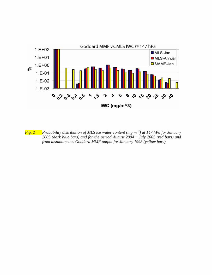
Fig. 2 Probability distribution of MLS ice water content (mg m–3) at 147 hPa for January 2005 (dark blue bars) and for the period August 2004 ~ July 2005 (red bars) and from instantaneous Goddard MMF output for January 1998 (yellow bars).

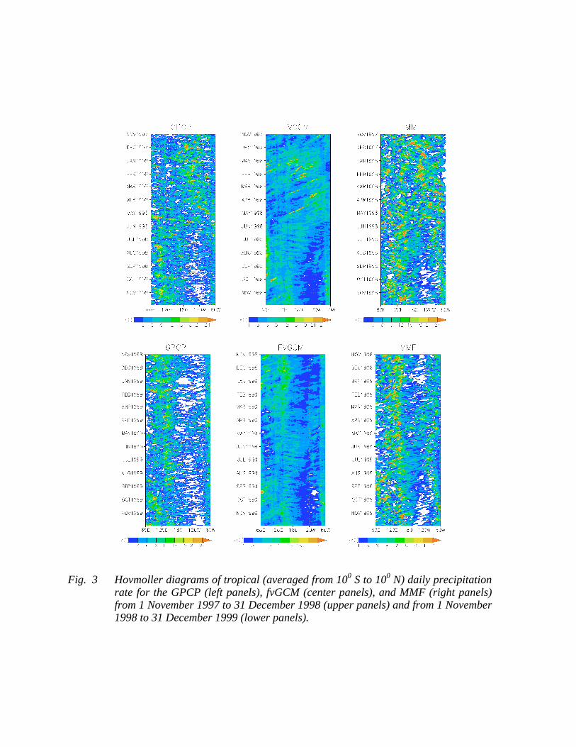
Fig. 3 Hovmoller diagrams of tropical (averaged from 100 S to 100 N) daily precipitation

rate for the GPCP (left panels), fvGCM (center panels), and MMF (right panels) from 1 November 1997 to 31 December 1998 (upper panels) and from 1 November 1998 to 31 December 1999 (lower panels).

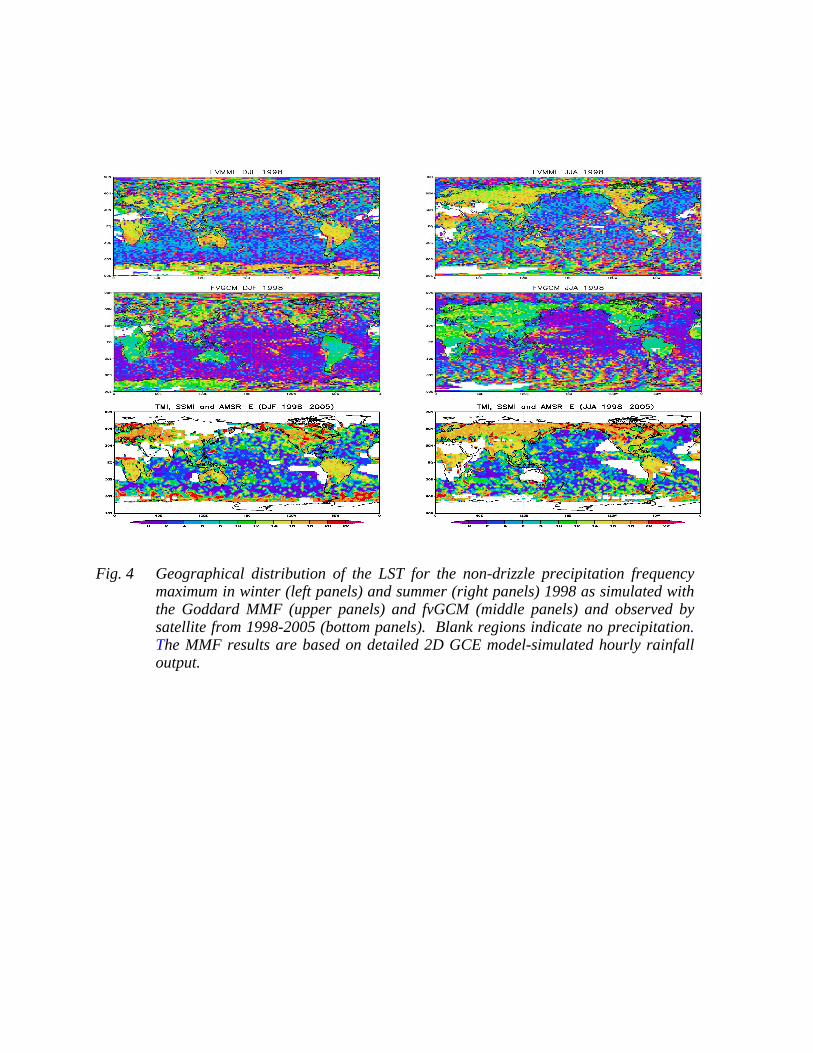
Fig. 4 Geographical distribution of the LST for the non-drizzle precipitation frequency

maximum in winter (left panels) and summer (right panels) 1998 as simulated with the Goddard MMF (upper panels) and fvGCM (middle panels) and observed by satellite from 1998-2005 (bottom panels). Blank regions indicate no precipitation. The MMF results are based on detailed 2D GCE model-simulated hourly rainfall output.

(b) (a) Fig. 5 (a) A global 2D CRM structure (single east-west orientation). Cyclic lateral

boundary conditions are replaced by direct coupling of the CRMs in neighboring GCM cells. (b) A quasi-3D CRM structure (from Randall et al. 2003b). Two orthogonal high-resolution CRM grids are extended to the walls of the GCM grid cells. In both of these new approaches, the effects of topography may be required in the embedded CRM.

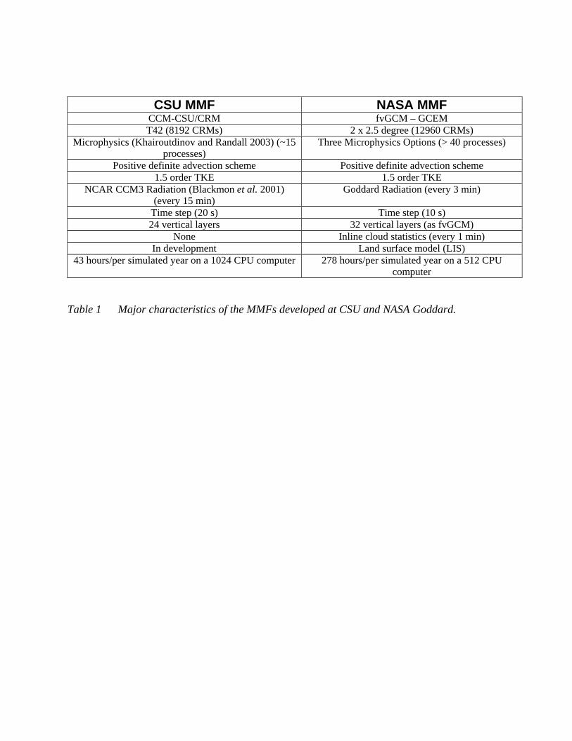
CSU MMF NASA MMF

CCM-CSU/CRM fvGCM – GCEM T42 (8192 CRMs) 2 x 2.5 degree (12960 CRMs)

Microphysics (Khairoutdinov and Randall 2003) (~15 processes)

Three Microphysics Options (> 40 processes)

Positive definite advection scheme Positive definite advection scheme 1.5 order TKE 1.5 order TKE

NCAR CCM3 Radiation (Blackmon et al. 2001) (every 15 min)

Goddard Radiation (every 3 min)

Time step (20 s) Time step (10 s) 24 vertical layers 32 vertical layers (as fvGCM)

None Inline cloud statistics (every 1 min) In development Land surface model (LIS)

43 hours/per simulated year on a 1024 CPU computer 278 hours/per simulated year on a 512 CPU computer

Table 1 Major characteristics of the MMFs developed at CSU and NASA Goddard.

Observation fvGCM Goddard MMF CCM CSU MMF

1998 2.65 3.07 3.17 2.88 2.84 1999 2.59 3.05 3.14 2.83 2.81

Table 2 The total rainfall amount for 1998 and 1999 from the fvGCM, Goddard MMF, CCM and CSU MMF. The observed rainfall (GPCP V3) is also shown for comparison.

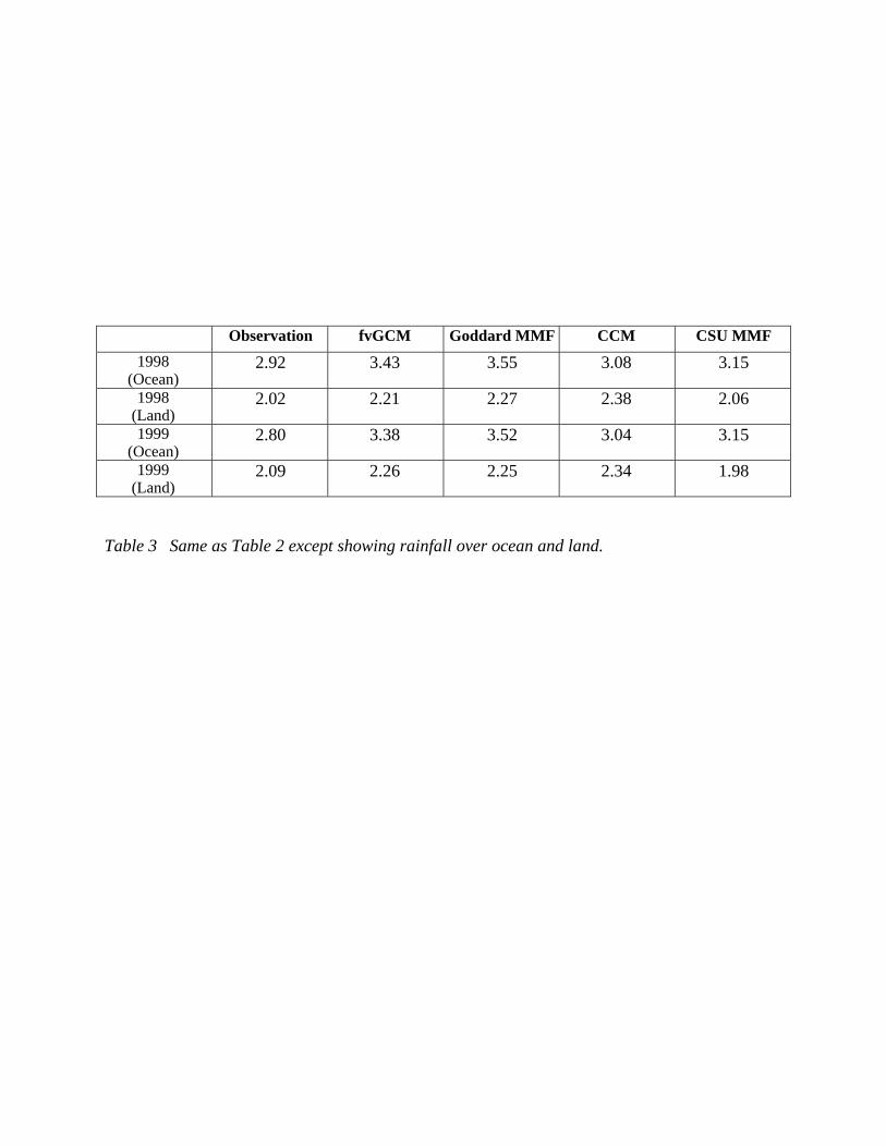
Observation fvGCM Goddard MMF CCM CSU MMF 1998

(Ocean) 2.92 3.43 3.55 3.08 3.15

1998 (Land)

2.02 2.21 2.27 2.38 2.06

1999 (Ocean)

2.80 3.38 3.52 3.04 3.15

1999 (Land)

2.09 2.26 2.25 2.34 1.98

Table 3 Same as Table 2 except showing rainfall over ocean and land.

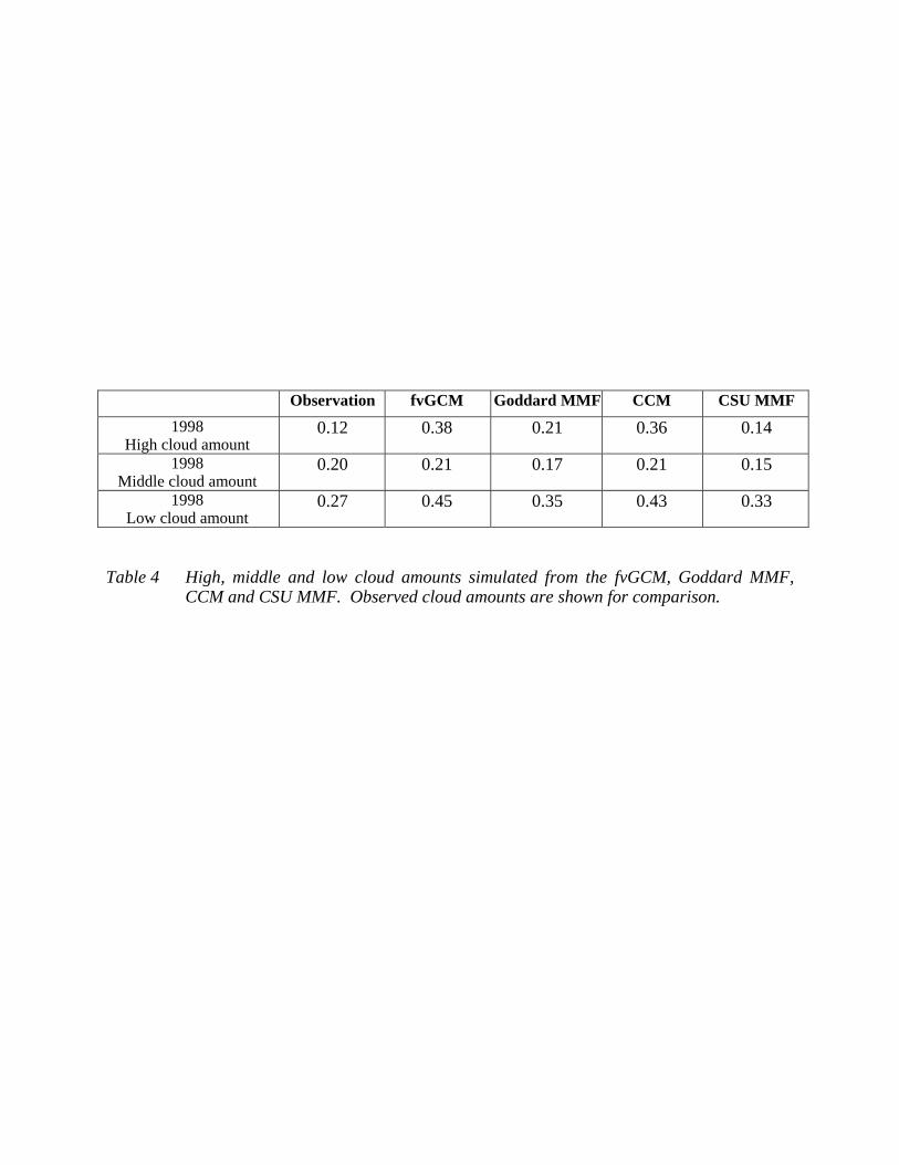
Observation fvGCM Goddard MMF CCM CSU MMF 1998

High cloud amount 0.12 0.38 0.21 0.36 0.14

1998 Middle cloud amount

0.20 0.21 0.17 0.21 0.15

1998 Low cloud amount

0.27 0.45 0.35 0.43 0.33

Table 4 High, middle and low cloud amounts simulated from the fvGCM, Goddard MMF,

CCM and CSU MMF. Observed cloud amounts are shown for comparison.