A Monte Carlo Analysis of Alternative Tests of … · A Monte Carlo Analysis of Alternative Tests of Contagion ... ity model test, and the Dungey, Fry, González-Hermosillo and Martin

A Monte Carlo Analysis of Alternative Testsof Contagion

Mardi Dungey+, Renée Fry+,Brenda González-Hermosillo∗ and Vance L. Martin#

+Australian National University∗International Monetary Fund#University of Melbourne

October 6, 2004

Abstract

The finite sample properties of various tests of contagion are inves-tigated using a range of Monte Carlo experiments. The tests consid-ered are the Forbes and Rigobon adjusted correlation test, the Faveroand Giavazzi outlier test, the Pesaran and Pick threshold test, the Bae,Karolyi and Stulz co-exceedance test, and the Dungey, Fry, González-Hermosillo and Martin factor test. Issues relating to potential biasesin testing for contagion, spurious contagion linkages, the identificationand measurement of common factors, the effects of alternative filteringmethods on the properties of test statistics, importance of structuralbreaks, and weak instrument issues, are also examined. The resultsshow that the Forbes and Rigobon test and the Pesaran and Pick testare unlikely to find evidence of contagion when it does exist, whilethe Favero and Giavazzi test and the Bae, Karolyi and Stulz test aremore likely to find contagion when it does not exist. The Dungey, Fry,Gonzalez-Hermosillo and Martin test yields reasonable power in mostof the experiments with moderate inflation of sizes.

1

1 Introduction

Contagion is broadly defined as an increase in the correlation between as-

set returns during a crisis period.1 There now exists a range of statistical

procedures to test for contagion. Some examples which are investigated in

detail here are the Forbes and Rigobon (2002) adjusted correlation test, the

Favero and Giavazzi (2002) outlier test, the Pesaran and Pick (2004) thresh-

old test, the Bae, Karolyi and Stulz (2003) co-exceedance test which contains

as a special case the Eichengreen, Rose and Wyplosz (1995, 1996) probabil-

ity model test, and the Dungey, Fry, González-Hermosillo and Martin (2002,

2004) factor test.2

There are two important distinguishing features of contagion tests. First,

they differ in the amount of information used to identify and test for con-

tagion. In all cases the testing frameworks represent tests of the impact of

shocks in one market on asset returns in another market during a crisis pe-

riod, with the main differences being how the shock is filtered. Forbes and

Rigobon (2002) and Dungey, Fry, González-Hermosillo and Martin (2002,

2004) use all of the information during the crisis period without any filtering

of the signals in either market. In contrast, Favero and Giavazzi (2002) and

Pesaran and Pick (2004) filter the size of shocks in the source market dur-

ing crisis periods by concentrating on the largest movements. Bae, Karolyi

and Stulz (2003) and Eichengreen, Rose and Wyplosz (1995, 1996) adopt a

1Further refinements of the definition of contagion are contained in Pericoli and Sbracia(2003) and the World Bank website on contagion. Also see Dornbusch, Park and Claessens(2000), and Dungey, Fry, González-Hermosillo and Martin (2004), for recent reviews.

2This list is by no means exhaustive, but it does perhaps represent the main tests usedin applied work with other tests providing important extensions or representing specialcases. The DCC test of Rigobon (2003) provides a multivariate analogue of the Forbesand Rigobon (2002) test. Implications of heteroskedasticity in testing for contagion areemphasised by Rigobon (2001) and Bekaert, Harvey and Ng (2005). Kaminsky and Rein-hart (2001), Mody and Taylor (2003) and Corsetti, Pericoli and Sbracia (2003), adopt alatent factor structure similar to the approach of Dungey, Fry, González-Hermosillo andMartin (2002). Finally, Lowell, Neu and Tong (1998) extend the probability model testof Eichengreen, Rose and Wyplosz (1995, 1996) to allow for both contemporanous andlagged relationships in the outliers.

2

similar approach, except that they filter all asset returns in all markets.

The second distinguishing feature of contagion tests is the treatment of

common shocks. It is important to identify common shocks which impact

upon all countries simultaneously (Pritsker (2002)), or within regions (Glick

and Rose (1999)). In either case, these shocks do not represent pure con-

tagion, but reflect the economic and financial linkages that exist between

countries during non-crisis periods. These linkages are sometimes referred

to as fundamentals based contagion (Kaminsky and Reinhart (2000), Dorn-

busch, Park and Claessens (2000)), but here the focus is on what is denoted

as pure contagion, or simply contagion from here on. A failure to model com-

mon shocks may result in tests of contagion being biased towards a positive

finding of contagion. There are two broad approaches to identifying common

shocks. The first is based on selecting a set of observable variables to act

as proxies for the common shocks (Forbes and Rigobon (2002); Bae, Karolyi

and Stulz (2003); and Eichengreen, Rose andWyplosz (1995, 1996)). Typical

choices include variables such as international interest rates, money supply

and trade variables. The second approach involves treating the common

shocks as latent and modelling their dynamics. Forbes and Rigobon (2002)

filter out the common shocks by using the estimated residuals from a VAR in

their contagion tests (see Baig and Goldfajn (1999) for a further application

of this approach). Favero and Giavazzi (2002) and Pesearan and Pick (2004)

also use a VAR to identify common shocks which, in turn, are included as

additional variables in a structural model. Dungey, Fry, González-Hermosillo

and Martin (2002, 2004) explicitly treat the common shocks as latent and

model their dynamics jointly with the potential linkages arising from conta-

gion.

Differences in the filtering of variables and in the procedures used to

model common shocks amount to differences in the information extracted

from the data to test for contagion. This has implications for the sampling

properties of the test statistics in terms of their power to identify contagion.

3

This is especially important in the contagion literature as often asymptotic

distribution theory is used when evaluating tests of contagion. However, this

strategy may be inappropriate in most, if not all empirical applications as the

sample sizes during crisis periods tend to be relatively small. In addition, the

problems of testing for contagion are exacerbated when increased volatility

in financial returns arises not just from contagion, but also from increased

volatility in either common or idiosyncratic factors. This additional source

of volatility represents a structural break in the market fundamentals which

may bias tests of contagion if not diagnosed correctly.

The aim of this paper is to investigate the finite sampling properties of

various tests of contagion using a range of Monte Carlo sampling experiments.

Both size and power comparisons are performed under various scenarios that

include increases in asset return volatility arising from both contagion and

structural breaks. In comparing the alternative testing methodologies, spe-

cial attention is devoted to identifying the impact of alternative filtering

strategies on the power properties of tests of contagion. Also investigated

are the different ways that common shocks are modelled and potential weak

instrument problems associated with the specification of structural models.3

The rest of the paper proceeds as follows. Section 2 provides some back-

ground statistics describing the nature and magnitude of various financial

crises. Section 3 provides some preliminary analysis for simulating finan-

cial crises which is used in the Monte Carlo experiments. An overview of

the alternative testing procedures investigated in the paper are discussed in

Section 4. Section 5 provides the finite sampling properties of these testing

procedures, while concluding comments are contained in Section 6.

3For some additional Monte Carlo evidence on tests of contagion, see Forbes andRigobon (2002), Peseran and Pick (2004), and Walti (2003).

4

2 Background

To identify some of the key characteristics of financial crises that will be used

in parameterising the DGP in the Monte Carlo experiments, Table 1 gives

the standard deviations of daily returns for three financial crises. The three

crises are the Tequila effect of December 1994 to March 1995, the Asian flu of

July 2997 to March 1988 and the Russian cold of August 1998 to November

1998.4 The data presented not only cover three different regions, but also

cover three different financial markets; namely, equity, currency and bond

markets. Inspection of the non-crisis and crisis standard deviations shows

that all crises are characterised by very large increases in volatility. The

extent of the change in volatility is further highlighted in Figure 1 which

gives time series plots of the three financial returns in each of the three

financial crises.

The increase in volatility during the crisis periods highlighted in Table

1 can be attributed to either an increase in volatility of the common and

idiosyncratic factors, or the result of contagion, or even both. Tests of conta-

gion need to separate between these two channels. These are the key issues

confronting tests of contagion.

A further issue that is important in testing for contagion concerns the

duration of crisis periods. These tend to be relatively short, for example the

Tequila and Russian examples in Table 1 are 54 and 62 days respectively.

The short nature of these crises suggests that asymptotic distribution theory

may not provide an accurate approximation to the finite sample distributions

of statistics used to test for contagion.

4Both the Tequila effect and the Asian flu had effects on both currency and equitymarkets. For purposes of illustration equity market data is used for the Tequila crisis andcurrencies for the Asian crisis.

5

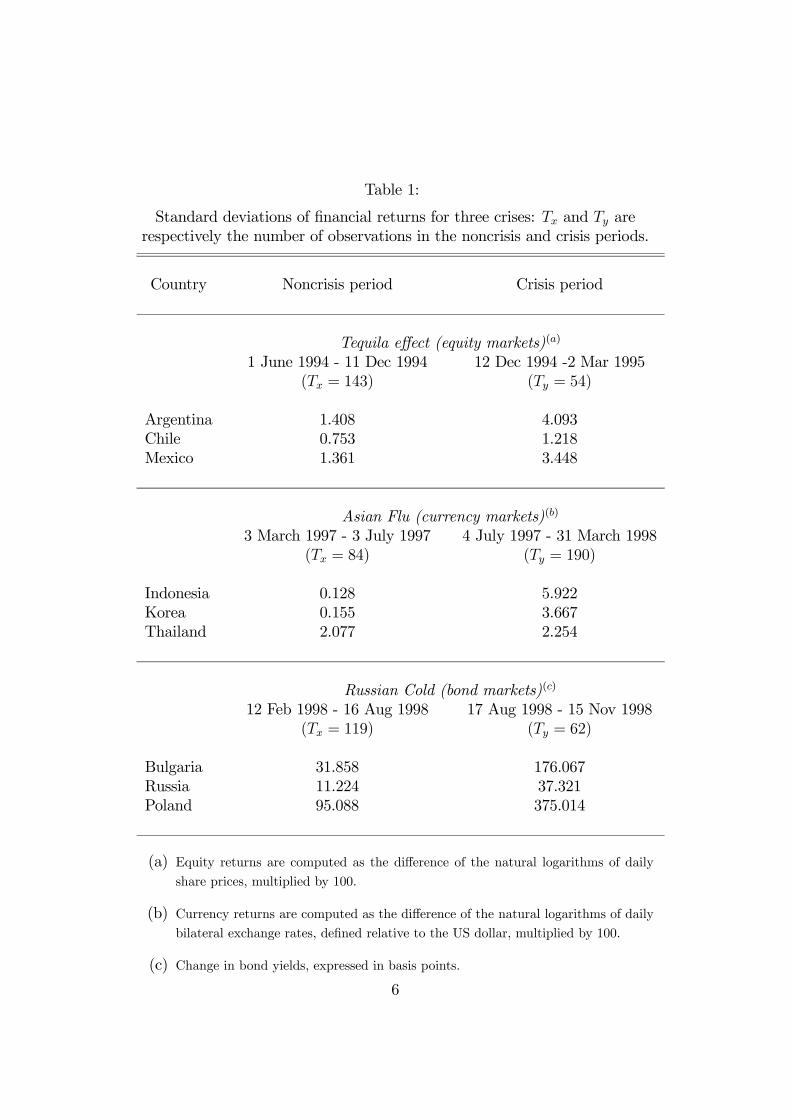
Table 1:

Standard deviations of financial returns for three crises: Tx and Ty arerespectively the number of observations in the noncrisis and crisis periods.

Country Noncrisis period Crisis period

Tequila effect (equity markets)(a)

1 June 1994 - 11 Dec 1994 12 Dec 1994 -2 Mar 1995(Tx = 143) (Ty = 54)

Argentina 1.408 4.093Chile 0.753 1.218Mexico 1.361 3.448

Asian Flu (currency markets)(b)

3 March 1997 - 3 July 1997 4 July 1997 - 31 March 1998(Tx = 84) (Ty = 190)

Indonesia 0.128 5.922Korea 0.155 3.667Thailand 2.077 2.254

Russian Cold (bond markets)(c)

12 Feb 1998 - 16 Aug 1998 17 Aug 1998 - 15 Nov 1998(Tx = 119) (Ty = 62)

Bulgaria 31.858 176.067Russia 11.224 37.321Poland 95.088 375.014

(a) Equity returns are computed as the difference of the natural logarithms of dailyshare prices, multiplied by 100.

(b) Currency returns are computed as the difference of the natural logarithms of dailybilateral exchange rates, defined relative to the US dollar, multiplied by 100.

(c) Change in bond yields, expressed in basis points.

6

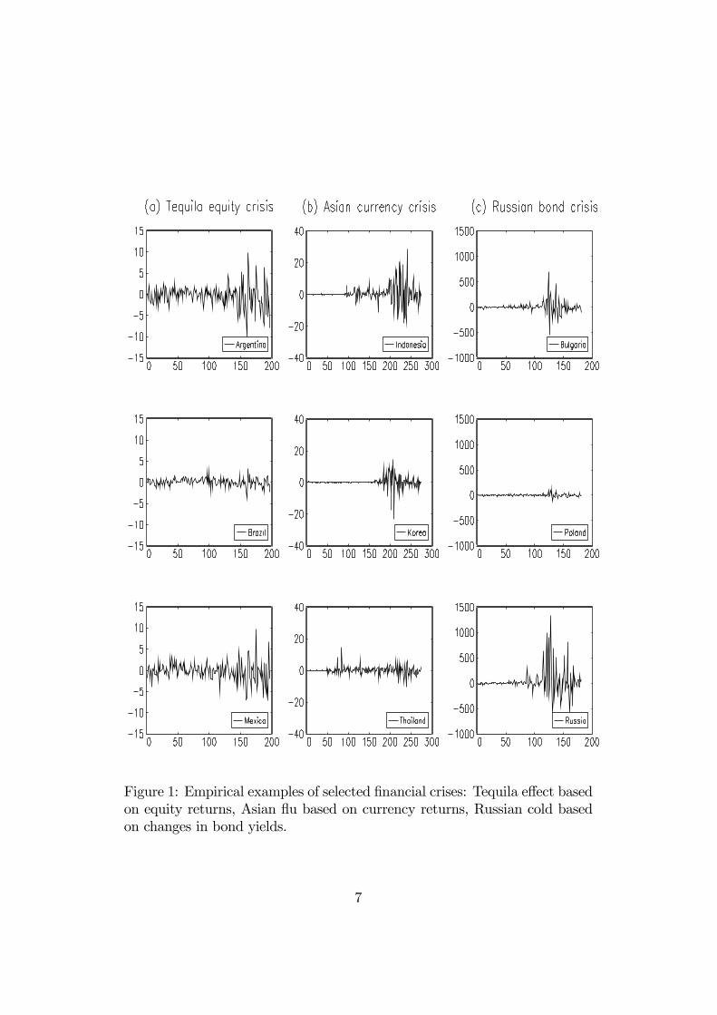
Figure 1: Empirical examples of selected financial crises: Tequila effect basedon equity returns, Asian flu based on currency returns, Russian cold basedon changes in bond yields.

7

3 Simulating Crises

In this section, a model of financial crises is developed by first outlining

financial market linkages in a tranquil, noncrisis period, and then extend-

ing the model to include crisis period linkages. The crisis model is based

on the framework of Dungey, Fry, González-Hermosillo and Martin (2002,

2004), which, in turn, is motivated by the class of factor models commonly

adopted in finance where the determinants of asset returns are decomposed

into common factors and idiosyncratic factors (see also Pericoli and Sbracia

(2003)). The model is couched in terms of the financial returns on assets

in three financial markets, although the analysis can easily be extended to

more markets. The model allows for increases in volatility arising from two

transmission mechanisms: structural shifts in the common and idiosyncratic

factors, and contagion. This model will serve as the basis for the DGP used

in the Monte Carlo experiments conducted in Section 4. An important fea-

ture of the model is that it highlights special features in the data which are

important in understanding the properties of contagion tests.

3.1 Noncrisis Model

The noncrisis model consists of a one (common) factor model where returns

(xi,t) are a function of a common factor (wt) and an idiosyncratic component

(ui,t)

xi,t = λiwt + φiui,t i = 1, 2, 3, (1)

where

wt ∼ N (0, 1) (2)

ui,t ∼ N (0, 1) i = 1, 2, 3, (3)

are assumed to be independent. The common factor captures systemic risk

which impacts upon asset returns with a loading of λi. The idiosyncratic

components capture unique aspects to each return, and impact upon asset

8

returns with a loading of φi. In a noncrisis period, the idiosyncratics rep-

resent potentially diversifiable non-systemic risk. In the special case where

λ1 = λ2 = λ3 = 0, the markets are segmented with volatility in asset returns

entirely driven by their respective idiosyncratic factors. The assumption

that the common and idiosyncratics are identically distributed can be re-

laxed by including autocorrelation and conditional volatility in the form of

GARCH; see for example Dungey, Martin and Pagan (2000), Dungey and

Martin (2004) and Bekaert, Harvey and Ng (2005).

3.2 Crisis Model

The crisis model is an extension of the noncrisis model in (1) to (3) by

allowing for a structural break in the world factor, as well as for increases in

asset return volatility resulting from an additional propagation mechanism

caused by contagion. This model is further extended in Section 4 to allow

for structural breaks in the idiosyncratic factors. To distinguish the crisis

period from the noncrisis period, returns in the crisis period are denoted

as yi,t. Contagion is assumed to transmit from country 1 to the remaining

two countries, countries 2 and 3. Additional dynamics can be included by

allowing for contagious feedback effects, provided that there are sufficient

identifying restrictions to be able to determine each propagation mechanism.

The factor structure during the crisis period is specified as

y1,t = λ1wt + φ1u1,t (4)

y2,t = λ2wt + φ2u2,t + δ2φ1u1,t (5)

y3,t = λ3wt + φ3u3,t + δ3φ1u1,t, (6)

where

wt ∼ N¡0, ω2

¢(7)

ui,t ∼ N (0, 1) i = 1, 2, 3. (8)

9

Contagion is defined as shocks originating in country 1, φ1u1,t = y1,t − λ1wt,

which impact upon the asset returns of countries 2 and 3, over and above

the contribution of the systemic factor (λiwt) and the country’s idiosyn-

cratic factor (φiui,t). The strength of the contagion channel is determined by

the parameters δ2 and δ3, in (5) and (6) for countries 2 and 3 respectively.

The transmission of volatility through the systemic factor is captured by the

structural break in the common factor (wt) , given by equation (7), where the

variance in the common factor increases from unity in the non-crisis period

to ω2 > 1, in the crisis period. For example, it may capture the impact of in-

creases in trading volumes or changes in the general risk profile of investors.

An implication of the model is that contagion adds to the level of nondi-

versifiable risk when diversification is needed most. This is highlighted by

equations (4) to (6) as the idiosyncratic of y1,t, given by u1,t, now represents

a common factor (nondiversifiable) during the crisis period; see also Walti

(2003) for further discussion of this point.

Let asset returns over the total period be denoted as zi,t, which are given

by concatenating the noncrisis and crisis period returns. Letting the sample

periods of the noncrisis and crisis periods be Tx and Ty, respectively, then

zi,t = (xi,1, xi,2, · · · , xi,Tx, yi,Tx+1, yi,Tx+2, · · · , yi,Tx+Ty)0, (9)

represents the full sample of asset returns for the ith country. The dynamics

of the common factor over the total period are summarised as

wt ∼½

N (0, 1) : t = 1, 2, · · · , TxN (0, ω2) : t = Tx + 1, Tx + 2, · · · , Tx + Ty

3.3 Covariance Structure

The specified model in (1) to (8) captures some of the key empirical fea-

tures of financial crises. To highlight these properties, consider the variance-

covariance matrices of returns for the two sample periods. Using the inde-

pendence assumption of the factors wt and ui,t, i = 1, 2, 3 in (2) and (3), the

10

variance-covariance matrix during the noncrisis period is obtained from (1)

Ωx =

⎡⎣ λ21 + φ21 λ1λ2 λ1λ3λ1λ2 λ22 + φ22 λ2λ3λ1λ3 λ2λ3 λ23 + φ23

⎤⎦ . (10)

Similarly, using (4) to (8) the variance-covariance matrix during the crisis

period is

Ωy =

⎡⎣ λ21ω2 + φ21 λ1λ2ω

2 + δ2φ21 λ1λ3ω

2 + δ3φ21

λ1λ2ω2 + δ2φ

21 λ22ω

2 + φ22 + δ22φ21 λ2λ3ω

2 + δ2δ3φ21

λ1λ3ω2 + δ3φ

21 λ2λ3ω

2 + δ2δ3φ21 λ23ω

2 + φ23 + δ22φ21

⎤⎦ . (11)

The proportionate increase in volatility of the source crisis country is

obtained directly from (10) and (11)

θ1 =V ar (y1,t)

V ar (x1,t)− 1 = λ21ω

2 + φ21λ21 + φ21

− 1 = λ21 (ω2 − 1)

λ21 + φ21. (12)

When there is no structural break (ω = 1) , there is no increase in volatility

in the source country (θ1 = 0). In this case, the increase in the volatility of

asset returns in countries 2 and 3 is solely the result of contagion, δi > 0, i =

2, 3. The general expressions for the proportionate increases in volatility in

countries 2 and 3 are respectively given by

θ2 =V ar (y2,t)

V ar (x2,t)− 1 = λ22ω

2 + φ22 + δ22φ21

λ22 + φ22− 1 = λ22 (ω

2 − 1) + δ22φ21

λ22 + φ22(13)

θ3 =V ar (y3,t)

V ar (x3,t)− 1 = λ23ω

2 + φ23 + δ23φ21

λ23 + φ23− 1 = λ23 (ω

2 − 1) + δ23φ21

λ23 + φ23.(14)

These expressions show that volatility can increase for two reasons: increased

volatility in the systemic factor¡λ2i (ω

2 − 1)¢and increased volatility arising

from contagion¡δ2iφ

21

¢. A fundamental requirement of any test of contagion is

to be able to identify the relative magnitudes of these two sources of increased

volatility.

To highlight further some of the features of the model, Table 2 presents

the variance-covariance matrices for the noncrisis (Ωx) and crisis (Ωy) periods

11

for a draw of the two experiments. The first experiment is where there is

contagion and no structural break in the common factor (ω = 1) . Figure

2(a) contains simulated time series of asset returns for the three countries

under this scenario. The sample sizes are Tx = 100 for the non-crisis period

and Ty = 50 for the crisis period. Asset return variances in countries 2 and

3 increase by a factor of 869% and 500%, respectively. These numbers are

comparable to the increases in the variances of financial returns for the three

historical financial crises reported in Table 1. By definition the volatility of

country 1 does not change with its variance equal to 20 in both periods.

The case where there is additional volatility in market fundamentals dur-

ing a crisis period (ω = 5), is given by Experiment 2 in Table 2. Figure 2(b)

contains simulated time series of asset returns for the three countries under

this scenario. The sample sizes are as before, namely, Tx = 100 for the non-

crisis period and Ty = 50 for the crisis period. Inspection of the variances

of all three countries show enormous increases in volatility during the crisis

period. Associated with the increases in the variances highlighted in Table

2, are also increases in the covariances. From (11), these increases in the

covariances arise from the increase in volatility of the market fundamentals

(λiλjω2) and of course contagion

¡δiδjφ

21

¢, ∀i, j with i 6= j, and δ1 = 1.

4 Review of Contagion Tests

This section presents the details of eight alternative tests of contagion whose

size and power properties are investigated in the Monte Carlo experiments

below.

4.1 Forbes and Rigobon Adjusted Correlation Test (FR1)

Forbes and Rigobon (2002) identify contagion as an increase in the corre-

lation of returns between noncrisis and crisis periods having adjusted for

market fundamentals and any increases in volatility of the source country.

12

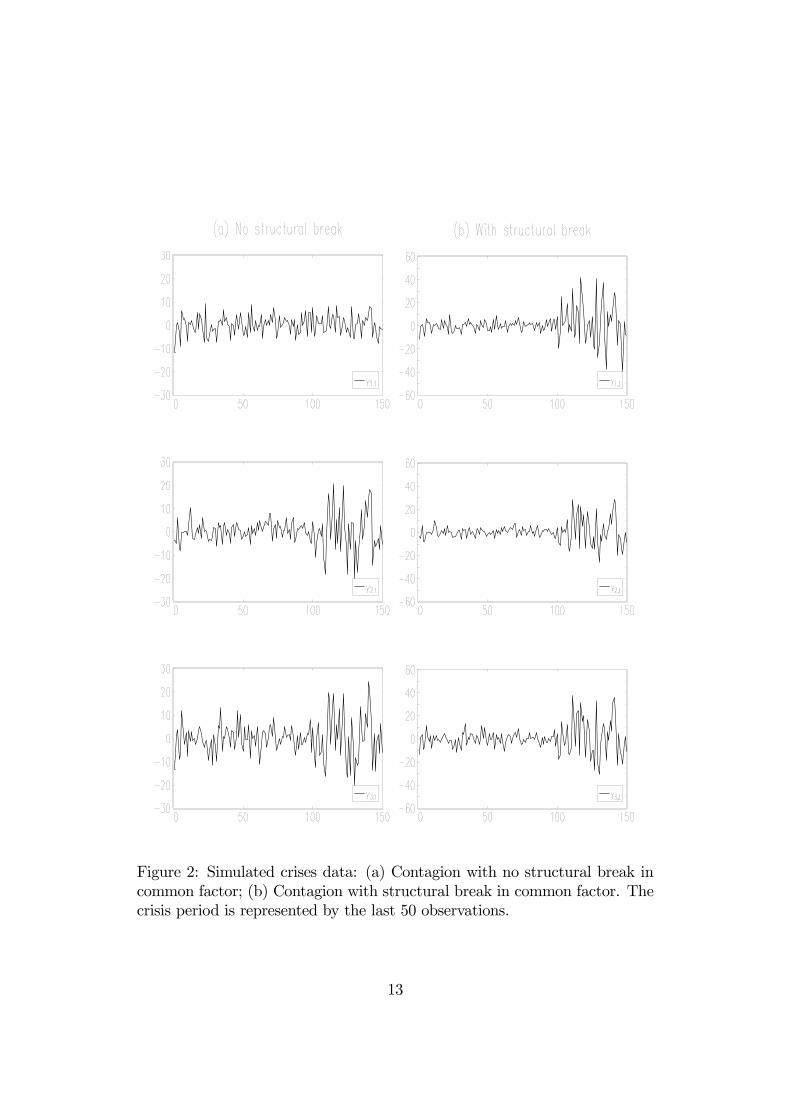
Figure 2: Simulated crises data: (a) Contagion with no structural break incommon factor; (b) Contagion with structural break in common factor. Thecrisis period is represented by the last 50 observations.

13

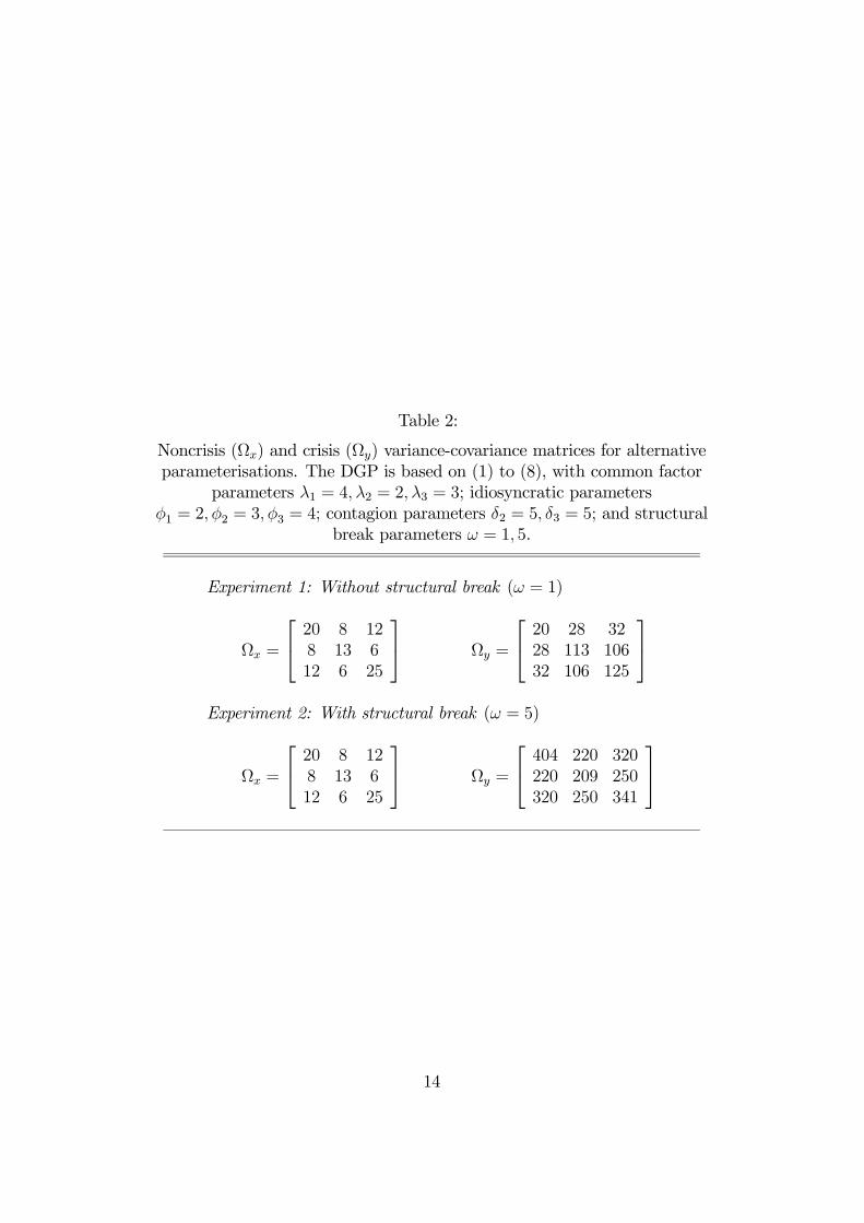
Table 2:

Noncrisis (Ωx) and crisis (Ωy) variance-covariance matrices for alternativeparameterisations. The DGP is based on (1) to (8), with common factor

parameters λ1 = 4, λ2 = 2, λ3 = 3; idiosyncratic parametersφ1 = 2, φ2 = 3, φ3 = 4; contagion parameters δ2 = 5, δ3 = 5; and structural

break parameters ω = 1, 5.

Experiment 1: Without structural break (ω = 1)

Ωx =

⎡⎣ 20 8 128 13 612 6 25

⎤⎦ Ωy =

⎡⎣ 20 28 3228 113 10632 106 125

⎤⎦Experiment 2: With structural break (ω = 5)

Ωx =

⎡⎣ 20 8 128 13 612 6 25

⎤⎦ Ωy =

⎡⎣ 404 220 320220 209 250320 250 341

⎤⎦

14

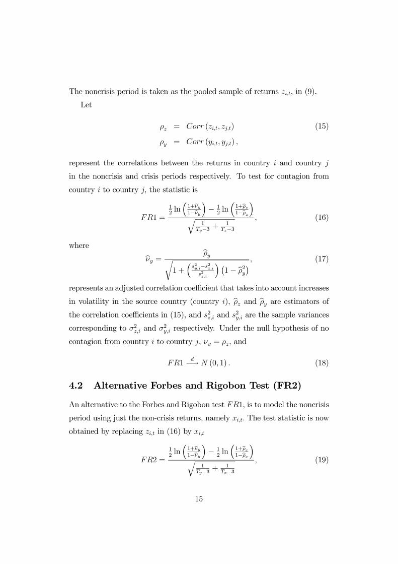
The noncrisis period is taken as the pooled sample of returns zi,t, in (9).

Let

ρz = Corr (zi,t, zj,t) (15)

ρy = Corr (yi,t, yj,t) ,

represent the correlations between the returns in country i and country j

in the noncrisis and crisis periods respectively. To test for contagion from

country i to country j, the statistic is

FR1 =

12ln³1+νy1−νy

´− 1

2ln³1+ρz1−ρz

´q

1Ty−3 +

1Tz−3

, (16)

where bνy = bρyr1 +

³s2y,i−s2z,i

s2z,i

´ ¡1− bρ2y¢ , (17)

represents an adjusted correlation coefficient that takes into account increases

in volatility in the source country (country i), bρz and bρy are estimators ofthe correlation coefficients in (15), and s2z,i and s2y,i are the sample variances

corresponding to σ2z,i and σ2y,i respectively. Under the null hypothesis of no

contagion from country i to country j, νy = ρz, and

FR1d−→ N (0, 1) . (18)

4.2 Alternative Forbes and Rigobon Test (FR2)

An alternative to the Forbes and Rigobon test FR1, is to model the noncrisis

period using just the non-crisis returns, namely xi,t. The test statistic is now

obtained by replacing zi,t in (16) by xi,t

FR2 =

12ln³1+νy1−νy

´− 1

2ln³1+ρx1−ρx

´q

1Ty−3 +

1Tx−3

, (19)

15

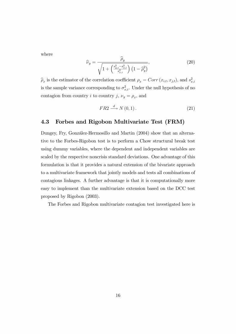
where bνy = bρyr1 +

³s2y,i−s2x,i

s2x,i

´ ¡1− bρ2y¢ , (20)

bρx is the estimator of the correlation coefficient ρx = Corr (xi,t, xj,t), and s2x,iis the sample variance corresponding to σ2x,i. Under the null hypothesis of no

contagion from country i to country j, νy = ρx, and

FR2d−→ N (0, 1) . (21)

4.3 Forbes and Rigobon Multivariate Test (FRM)

Dungey, Fry, González-Hermosillo and Martin (2004) show that an alterna-

tive to the Forbes-Rigobon test is to perform a Chow structural break test

using dummy variables, where the dependent and independent variables are

scaled by the respective noncrisis standard deviations. One advantage of this

formulation is that it provides a natural extension of the bivariate approach

to a multivariate framework that jointly models and tests all combinations of

contagious linkages. A further advantage is that it is computationally more

easy to implement than the multivariate extension based on the DCC test

proposed by Rigobon (2003).

The Forbes and Rigobon multivariate contagion test investigated here is

16

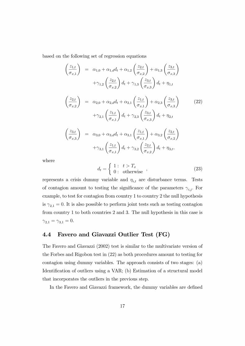
based on the following set of regression equationsµz1,tσx,1

¶= α1,0 + α1,ddt + α1,2

µz2,tσx,2

¶+ α1,3

µz3,tσx,3

¶+γ1,2

µz2,tσx,2

¶dt + γ1,3

µz3,tσx,3

¶dt + η1,t

µz2,tσx,2

¶= α2,0 + α2,ddt + α2,1

µz1,tσx,1

¶+ α2,3

µz3,tσx,3

¶(22)

+γ2,1

µz1,tσx,1

¶dt + γ2,3

µz3,tσx,3

¶dt + η2,t

µz3,tσx,3

¶= α3,0 + α3,ddt + α3,1

µz1,tσx,1

¶+ α3,2

µz2,tσx,2

¶+γ3,1

µz1,tσx,1

¶dt + γ3,2

µz2,tσx,2

¶dt + η3,t,

where

dt =

½1 : t > Tx0 : otherwise

, (23)

represents a crisis dummy variable and ηi,t are disturbance terms. Tests

of contagion amount to testing the significance of the parameters γi,j. For

example, to test for contagion from country 1 to country 2 the null hypothesis

is γ2,1 = 0. It is also possible to perform joint tests such as testing contagion

from country 1 to both countries 2 and 3. The null hypothesis in this case is

γ2,1 = γ3,1 = 0.

4.4 Favero and Giavazzi Outlier Test (FG)

The Favero and Giavazzi (2002) test is similar to the multivariate version of

the Forbes and Rigobon test in (22) as both procedures amount to testing for

contagion using dummy variables. The approach consists of two stages: (a)

Identification of outliers using a VAR; (b) Estimation of a structural model

that incorporates the outliers in the previous step.

In the Favero and Giavazzi framework, the dummy variables are defined

17

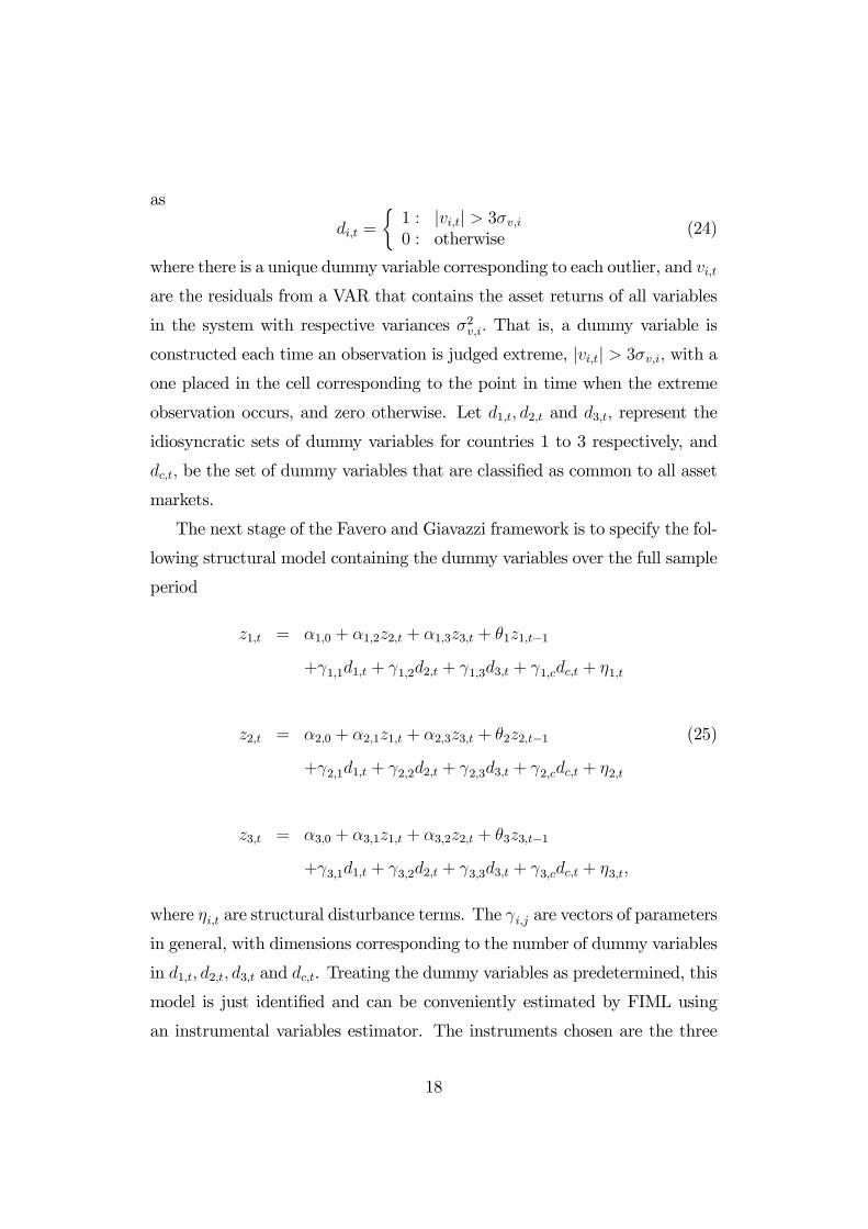
as

di,t =

½1 : |vi,t| > 3σv,i0 : otherwise

(24)

where there is a unique dummy variable corresponding to each outlier, and vi,t

are the residuals from a VAR that contains the asset returns of all variables

in the system with respective variances σ2v,i. That is, a dummy variable is

constructed each time an observation is judged extreme, |vi,t| > 3σv,i, with aone placed in the cell corresponding to the point in time when the extreme

observation occurs, and zero otherwise. Let d1,t, d2,t and d3,t, represent the

idiosyncratic sets of dummy variables for countries 1 to 3 respectively, and

dc,t, be the set of dummy variables that are classified as common to all asset

markets.

The next stage of the Favero and Giavazzi framework is to specify the fol-

lowing structural model containing the dummy variables over the full sample

period

z1,t = α1,0 + α1,2z2,t + α1,3z3,t + θ1z1,t−1

+γ1,1d1,t + γ1,2d2,t + γ1,3d3,t + γ1,cdc,t + η1,t

z2,t = α2,0 + α2,1z1,t + α2,3z3,t + θ2z2,t−1 (25)

+γ2,1d1,t + γ2,2d2,t + γ2,3d3,t + γ2,cdc,t + η2,t

z3,t = α3,0 + α3,1z1,t + α3,2z2,t + θ3z3,t−1

+γ3,1d1,t + γ3,2d2,t + γ3,3d3,t + γ3,cdc,t + η3,t,

where ηi,t are structural disturbance terms. The γi,j are vectors of parameters

in general, with dimensions corresponding to the number of dummy variables

in d1,t, d2,t, d3,t and dc,t. Treating the dummy variables as predetermined, this

model is just identified and can be conveniently estimated by FIML using

an instrumental variables estimator. The instruments chosen are the three

18

lagged returns, the constant and all dummy variables. Tests of contagion are

based on testing the γi,j ∀i 6= j parameters.

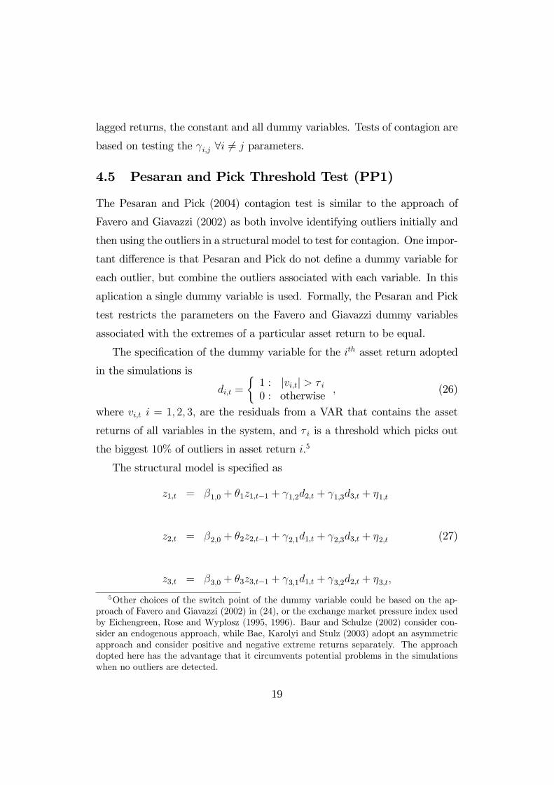
4.5 Pesaran and Pick Threshold Test (PP1)

The Pesaran and Pick (2004) contagion test is similar to the approach of

Favero and Giavazzi (2002) as both involve identifying outliers initially and

then using the outliers in a structural model to test for contagion. One impor-

tant difference is that Pesaran and Pick do not define a dummy variable for

each outlier, but combine the outliers associated with each variable. In this

aplication a single dummy variable is used. Formally, the Pesaran and Pick

test restricts the parameters on the Favero and Giavazzi dummy variables

associated with the extremes of a particular asset return to be equal.

The specification of the dummy variable for the ith asset return adopted

in the simulations is

di,t =

½1 : |vi,t| > τ i0 : otherwise

, (26)

where vi,t i = 1, 2, 3, are the residuals from a VAR that contains the asset

returns of all variables in the system, and τ i is a threshold which picks out

the biggest 10% of outliers in asset return i.5

The structural model is specified as

z1,t = β1,0 + θ1z1,t−1 + γ1,2d2,t + γ1,3d3,t + η1,t

z2,t = β2,0 + θ2z2,t−1 + γ2,1d1,t + γ2,3d3,t + η2,t (27)

z3,t = β3,0 + θ3z3,t−1 + γ3,1d1,t + γ3,2d2,t + η3,t,

5Other choices of the switch point of the dummy variable could be based on the ap-proach of Favero and Giavazzi (2002) in (24), or the exchange market pressure index usedby Eichengreen, Rose and Wyplosz (1995, 1996). Baur and Schulze (2002) consider con-sider an endogenous approach, while Bae, Karolyi and Stulz (2003) adopt an asymmetricapproach and consider positive and negative extreme returns separately. The approachdopted here has the advantage that it circumvents potential problems in the simulationswhen no outliers are detected.

19

where ηi,t are structural disturbance terms. Unlike Favero and Giavazzi,

Pesaran and Pick treat the dummy variables as endogenous. In which case

the model is just identified and can be conveniently estimated by FIML using

an instrumental variables estimator. The instruments chosen are the three

lagged returns, and the constant. Tests of contagion are based on testing the

parameters γi,j, ∀i 6= j.

4.6 Adjusted Pesaran and Pick Threshold Test (PP2)

An alternative version of the Pesaran and Pick contagion test investigated in

the Monte Carlo experiments is to estimate (27) by OLS and not adjust for

any simultaneity bias. This form of the test is motivated by the possibility

of weak instruments and its consequences for testing for contagion. These

issues are dicussed further below.

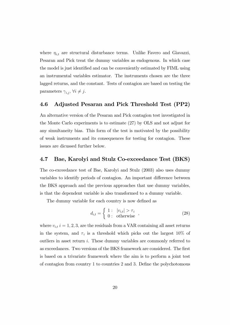
4.7 Bae, Karolyi and Stulz Co-exceedance Test (BKS)

The co-exceedance test of Bae, Karolyi and Stulz (2003) also uses dummy

variables to identify periods of contagion. An important difference between

the BKS approach and the previous approaches that use dummy variables,

is that the dependent variable is also transformed to a dummy variable.

The dummy variable for each country is now defined as

di,t =

½1 : |vi,t| > τ i0 : otherwise

, (28)

where vi,t i = 1, 2, 3, are the residuals from a VAR containing all asset returns

in the system, and τ i is a threshold which picks out the largest 10% of

outliers in asset return i. These dummy variables are commonly referred to

as exceedances. Two versions of the BKS framework are considered. The first

is based on a trivariate framework where the aim is to perform a joint test

of contagion from country 1 to countries 2 and 3. Define the polychotomous

20

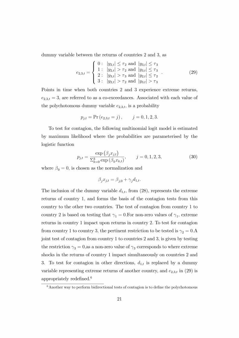
dummy variable between the returns of countries 2 and 3, as

e2,3,t =

⎧⎪⎪⎨⎪⎪⎩0 : |y2,t| ≤ τ 2 and |y3,t| ≤ τ 31 : |y2,t| > τ 2 and |y3,t| ≤ τ 32 : |y3,t| > τ 3 and |y2,t| ≤ τ 23 : |y2,t| > τ 2 and |y3,t| > τ 3

. (29)

Points in time when both countries 2 and 3 experience extreme returns,

e2,3,t = 3, are referred to as a co-exceedances. Associated with each value of

the polychotomous dummy variable e2,3,t, is a probability

pj,t = Pr (e2,3,t = j) , j = 0, 1, 2, 3.

To test for contagion, the following multinomial logit model is estimated

by maximum likelihood where the probabilities are parameterised by the

logistic function

pj,t =exp

¡βjxj,t

¢Σ3k=0 exp (βkxk,t)

, j = 0, 1, 2, 3, (30)

where β0 = 0, is chosen as the normalization and

βjxj,t = βj,0 + γjd1,t.

The inclusion of the dummy variable d1,t, from (28), represents the extreme

returns of country 1, and forms the basis of the contagion tests from this

country to the other two countries. The test of contagion from country 1 to

country 2 is based on testing that γ1 = 0.For non-zero values of γ1, extreme

returns in country 1 impact upon returns in country 2. To test for contagion

from country 1 to country 3, the pertinent restriction to be tested is γ2 = 0.A

joint test of contagion from country 1 to countries 2 and 3, is given by testing

the restriction γ3 = 0,as a non-zero value of γ3 corresponds to where extreme

shocks in the returns of country 1 impact simultaneously on countries 2 and

3. To test for contagion in other directions, d1,t is replaced by a dummy

variable representing extreme returns of another country, and e2,3,t in (29) is

appropriately redefined.6

6Another way to perform bidirectional tests of contagion is to define the polychotomous

21

4.8 Dungey, Fry, González-Hermosillo andMartin Fac-tor Test (DFGM)

Dungey, Fry, González-Hermosillo and Martin (2002, 2004) specify a latent

factor model containing both common and idiosyncratic factors. Contagion

occurs where an idiosyncratic shock in one asset market impacts upon the

returns in another asset market. An important feature of this model is that

all channels that transmit volatility across countries are modelled jointly.

A further feature is that the common factors do not need to be identified

explicitly, but rather are treated as latent processes and identified by the

comovements of asset returns.

The form of the latent factor model is an extension of the DGP given by

equations (1) to (8), which allows for testing of contagion between countries

2 and 3. The noncrisis model is

xi,t = λiwt + φiui,t i = 1, 2, 3, (31)

where

wt ∼ N (0, 1) (32)

ui,t ∼ N (0, 1) i = 1, 2, 3, (33)

and the crisis model is

y1,t = λ1wt + φ1u1,t (34)

y2,t = λ2wt + φ2u2,t + γ2,1φ1u1,t + γ2,3φ3u3,t (35)

y3,t = λ3wt + φ3u3,t + γ3,1φ1u1,t + γ3,2φ2u2,t, (36)

where

wt ∼ N¡0, ω2

¢(37)

ui,t ∼ N (0, 1) i = 1, 2, 3. (38)

dummy variable e2,3,t in (29), simply in terms of one variable; that is, define a binarydummy variable. This is also the approach adopted by Eichengreen, Rose and Wyplosz(1995, 1996), except that they specify the underlying distribution to be normal, resultingin the use of a probit model.

22

The parameters of the model are estimated by generalised method of mo-

ments (GMM) by matching the theoretical variances and covariances of equa-

tions (31) and (38) with the corresponding empirical variance-covariances in

the non-crisis and crisis periods. The number of unknown parameters is 11©λ1, λ2, λ3, φ1, φ2, φ3, ω, γ2,1, γ2,3, γ3,1, γ3,2

ª,

and the number of empirical moments is 12, which correspond to the 3 vari-

ances and covariances obtained for each of the noncrisis and crisis periods.

In essence, the 6 empirical moments from the noncrisis period identify the

parameters λ1, λ2, λ3, φ1, φ2, φ3 . This now leaves©ω, γ2,1, γ2,3, γ3,1, γ3,2

ªto

be identified using the 6 empirical moments from the crisis period, thereby

resulting in an overidentifed system.

The contagion tests are based on testing the null hypothesis γi,j = 0. For

example to test for contagion from country 1 to country 2, the restriction is

γ2,1 = 0. To test for contagion from country 2 to country 3, the restriction is

γ3,2 = 0.An overall test of contagion is given by jointly testing the restrictions

γ2,1 = γ2,3 = γ3,1 = γ3,2 = 0.

4.9 Discussion

4.9.1 Biasedness in testing for contagion using correlation

An important feature of the Forbes and Rigobon contagion tests (FR1 and

FR2), is that they are based on testing the difference in bivariate correlations

between noncrisis and crisis periods. Using the expressions for the variance-

covariance matrices in (10) and (11), the difference in the two correlations

between countries 1 and 2 is immediately given by

ρy1,t,y2,t − ρx1,t,x2,t =λ1λ2ω

2 + δ2φ21p

λ21ω2 + φ21

pλ22ω

2 + φ22 + δ22φ21

− λ1λ2pλ21 + φ21

pλ22 + φ22

.

(39)

Some insight into this expression is obtained by looking at what happens as

contagion continuously increases (with δ2 replaced by δ) and when there is

23

no structural break in the common factor (ω = 1)

limδ→∞

³ρy1,t,y2,t − ρx1,t,x2,t

´= lim

δ→∞

Ãλ1λ2ω

2 + δφ21pλ21 + φ21

pλ22 + φ22 + δ2φ21

!− λ1λ2p

λ21 + φ21pλ22 + φ22

= limδ→∞

⎛⎝ λ1λ2ω2/δ + φ21p

λ21 + φ21

qλ22/δ

2 + φ22/δ2 + φ21

⎞⎠− λ1λ2p

λ21 + φ21pλ22 + φ22

=φ1p

λ21 + φ21− λ1λ2p

λ21 + φ21pλ22 + φ22

=1p

λ21 + φ21

Ãφ1 −

λ1λ2pλ22 + φ22

!.

For “high” levels of contagion, the correlation in the noncrisis period can

exceed the crisis period correlation when

φ1 −λ1λ2pλ22 + φ22

< 0

or

1 +

µφ2λ2

¶2<

µλ1φ1

¶2.

Thus the key magnitudes are the relative sizes of the loadings of the common

factor (λi) to the idiosyncratic factor (φi) for the two assets.

Figure 3(a) gives the difference in the crisis and noncrisis correlations

between countries 1 and 2 using (39), for alternative values of the contagion

parameter (δ = δ1 = δ2) and the structural break parameter (ω) , where the

values of the remaining parameters are given by

λ1 = 4, λ2 = 2, λ3 = 3, φ1 = 2, φ2 = 3, φ3 = 4.

This figure shows that when there is no structural break in the common

factor (ω = 1) , a value of δ close to 20, causes the correlation during the crisis

24

period to be marginally less than it is for the noncrisis period. This result

is at odds with the initial idea of testing for contagion based on identifying

a significant increase in correlation during a crisis period. That is, the null

hypothesis is usually taken as one-sided when testing for contagion based

on correlation analysis; see also the discussion in Billio and Pelizzon (2003).

However, this phenomenon is not uncommon when computing the correlation

structure of asset returns during financial crises.7 What this result shows is

that looking at simple correlations can be highly misleading when attempting

to identify evidence of contagion. Even though for certain parameterisations

the correlation during the crisis period is less than it is for the noncrisis

period, Figure 3(a) highlights that this is not inconsistent with the presence

of contagion (δ > 0). From a testing point of view, this result also suggests

that in testing for contagion based on correlation analysis, the power of the

test statistic to detect contagion may not be monotonic over the parameter

space. In fact, this test is not guaranteed to be unbiased, especially for

one-sided null hypotheses.8

4.9.2 Spuriousness in testing for contagion

Contagion tests based on bivariate analysis such as the Forbes and Rigobon

tests (FR1 and FR2), can potentially yield spurious contagious linkages be-

tween variables as a result of a common factor. This point is highlighted in

Figure 3(b) which gives the difference in the crisis and noncrisis correlations

between countries 2 and 3 for alternative values of the contagion parame-

ter (δ = δ1 = δ2) and the structural break parameter (ω) . As the strength of

contagion increases (δ > 0) , the correlation between the two asset returns in-

7For example, Forbes and Rigobon (2002) find crisis correlations less than non-crisiscorrelations during the Hong Kong equity crisis, the Mexican peso crisis, and the 1987 USstock market crash. Baig and Goldfajn (1999) find large movements in correlations duringthe Asian currency crisis by computing correlations over a rolling window.

8The phenonemon that noncrisis correlations can exceed crisis correlations suggeststhat choosing a crisis sample on the basis of the correlation exceeding that of surroundingperiods is inappropriate.

25

creases. This increase in correlation is purely spurious as it arises from both

variables being affected by a common factor, namely shocks from country 1

asset returns.

4.9.3 Structural breaks

Loretan and English (2000) and Forbes and Rigobon (2002) emphasise the

problems of structural breaks in testing for contagion. This problem is high-

lighted in Figures 3(a) and 3(b) for the case of a structural break in the

common factor (ω > 1). Increases in the strength of the structural break ac-

centuates the differences in the noncrisis and crisis correlations. Figure 3(a)

also shows that for greater levels of contagion, the switch in the magnitides

of the correlations in the two sample periods becomes even more marked.

Forbes and Rigobon (2002) in designing their test focus on robustifying

the test statistic to structural breaks in the idiosyncratic factor of the source

of the crisis. Dungey, Fry, González-Hermosillo and Martin (2004) show

that an alternative way to correct for this form of structural break and test

for contagion is to perform a Chow test with the pertinent dummy variable

defined over the crisis period. An important question then is whether the test

is also robust to other forms of structural breaks, such as structural breaks

in the common factors.

4.9.4 Weak instruments

The Favero and Giavazzi test (FG) and the Pesaran and Pick test (PP1)

both require identifying key parameters using instruments based on lagged

variables. In applications using interest rates, as in the original Favero and

Giavazzi application, the strong correlation in the data should produce strong

instruments. However, for applications using asset returns, as in the appli-

cation by Walti (2003), the low levels of correlations in the data are unlikely

to produce instruments with suitable properties. The effect of weak instru-

ments will result in the variance of the sampling distributions of the test

26

statistics having fat-tails, with asymptotic distribution theory providing a

poor approximation to the finite sample distribution. The end result can be

expected to lead to a significant loss in power in testing for contagion. It may

work out that the bias caused by ignoring the simultaneity bias, may be of a

much smaller magnitide than the bias caused by working with weak instru-

ments. In which case, the adjusted Pesaran and Pick test (PP2) may yield

better sampling properties than the PP1 test, which corrects for simultaneity

bias using an IV estimator.

4.9.5 Information loss from filtering

The Favero and Giavazzi test (FG), the Pesaran and Pick tests (PP1 and

PP2) and the Bae, Karolyi and Stulz test (BKS), all use a filter to identify

large shocks. This contrasts with the four tests (FR1, FR2, FRMand DFGM)

which use all of the information in the sample to test for contagion. In

general, the filtering methods represent a loss of information which can be

expected to result in a loss of power. The extent of the loss in power can be

identified using a range of Monte Carlo experiments.

4.9.6 Modelling of common factors

An important difference in tests of contagion is the treatment of the com-

mon factor. The DFGM test assumes that it is latent with its contribution

formally modelled jointly with the known variables in the system. Another

approach is to estimate a VAR and purge any common factors by using the

residuals in the contagion tests. This approach will be successful if there is

strong autocorrelation in the data. In the case of asset returns, this will not

necessarily be the case.

4.9.7 Incorrect assumptions

One advantage of the version of the alternative form of the Forbes and

Rigobon test (FR2) is that the assumption that the variances of the correla-

27

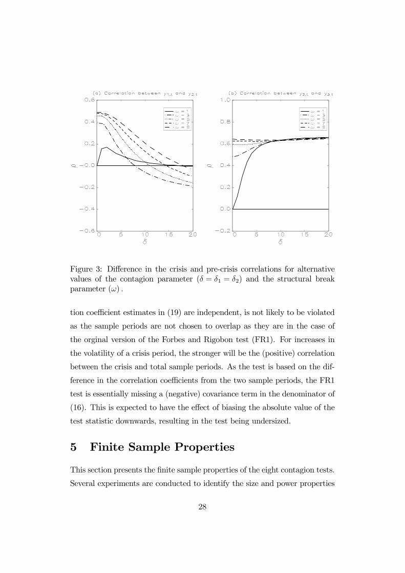
Figure 3: Difference in the crisis and pre-crisis correlations for alternativevalues of the contagion parameter (δ = δ1 = δ2) and the structural breakparameter (ω) .

tion coefficient estimates in (19) are independent, is not likely to be violated

as the sample periods are not chosen to overlap as they are in the case of

the orginal version of the Forbes and Rigobon test (FR1). For increases in

the volatility of a crisis period, the stronger will be the (positive) correlation

between the crisis and total sample periods. As the test is based on the dif-

ference in the correlation coefficients from the two sample periods, the FR1

test is essentially missing a (negative) covariance term in the denominator of

(16). This is expected to have the effect of biasing the absolute value of the

test statistic downwards, resulting in the test being undersized.

5 Finite Sample Properties

This section presents the finite sample properties of the eight contagion tests.

Several experiments are conducted to identify the size and power properties

28

of the test statistics under various scenarios.

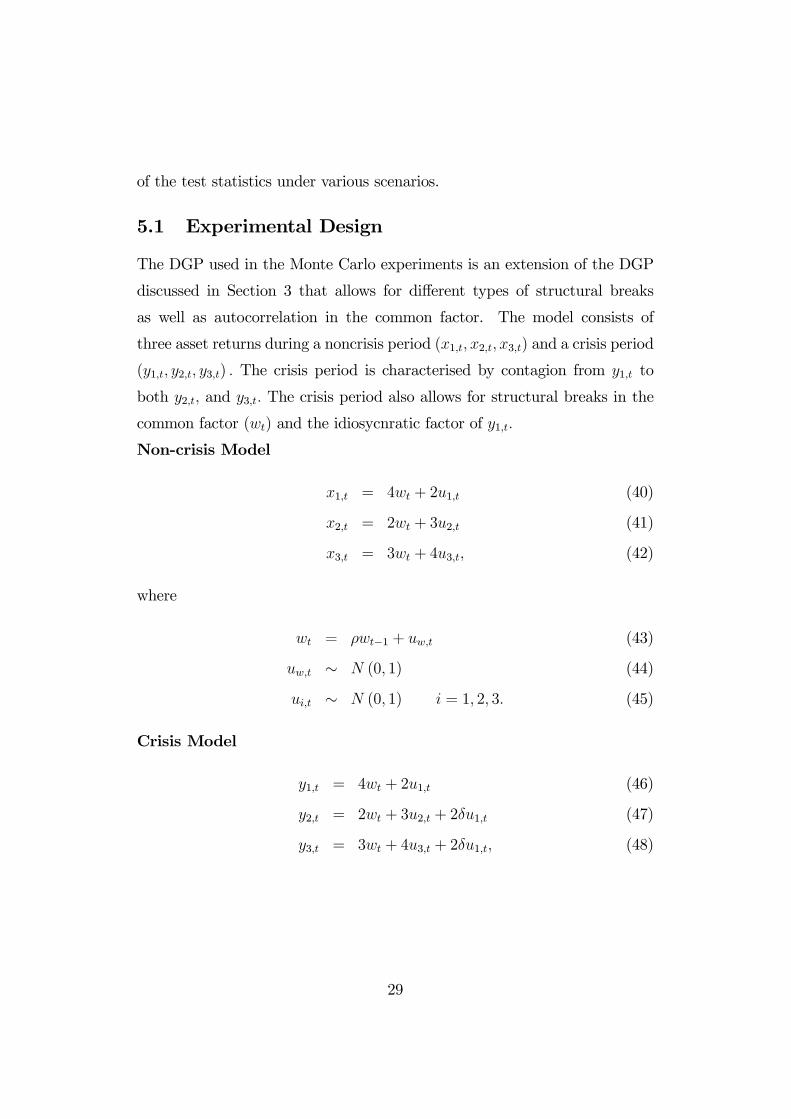
5.1 Experimental Design

The DGP used in the Monte Carlo experiments is an extension of the DGP

discussed in Section 3 that allows for different types of structural breaks

as well as autocorrelation in the common factor. The model consists of

three asset returns during a noncrisis period (x1,t, x2,t, x3,t) and a crisis period

(y1,t, y2,t, y3,t) . The crisis period is characterised by contagion from y1,t to

both y2,t, and y3,t. The crisis period also allows for structural breaks in the

common factor (wt) and the idiosycnratic factor of y1,t.

Non-crisis Model

x1,t = 4wt + 2u1,t (40)

x2,t = 2wt + 3u2,t (41)

x3,t = 3wt + 4u3,t, (42)

where

wt = ρwt−1 + uw,t (43)

uw,t ∼ N (0, 1) (44)

ui,t ∼ N (0, 1) i = 1, 2, 3. (45)

Crisis Model

y1,t = 4wt + 2u1,t (46)

y2,t = 2wt + 3u2,t + 2δu1,t (47)

y3,t = 3wt + 4u3,t + 2δu1,t, (48)

29

where

wt = ρwt−1 + uw,t (49)

uw,t ∼ N¡0, ω2

¢(50)

u1,t ∼ N¡0, κ2

¢(51)

ui,t ∼ N (0, 1) i = 2, 3. (52)

The strength of contagion is controlled by the parameter δ in (47) and

(48). The parameter values chosen in the Monte carlo experiments are

δ = 0, 1, 2, 5, 10 . (53)

A value of δ = 0, represents no contagion and is used to examine the size

properties of the test statistics in small samples when the asymptotic critical

values are used. Values of δ > 0, are used to examine the power properties

of the contagion tests using size-adjusted critical values.

Two types of structural breaks are investigated. The first is a structural

break in the common factor wt. The parameter values chosen are

ω = 1, 5 , (54)

where ω = 1, represents no structural break in the common factor during the

crisis period. The second is a structural break in the idiosyncratic factor of

y1,t, namely u1,t. The parameter values are

κ = 1, 5 , (55)

where κ = 1, represents no structural break in the idiosyncratic factor during

the crisis period.

Five Monte Carlo experiments are performed which are summarised in

Table 3. For each experiment, six hypotheses are tested (Table 4) using

eight alternative contagion tests (Table 5). The FR1 and FR2 tests are used

to test the first four hypotheses in Table 4, but not the two joint hypotheses

30

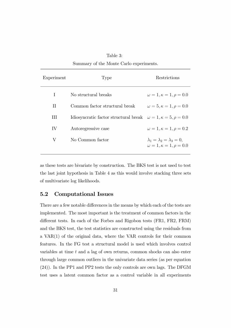
Table 3:

Summary of the Monte Carlo experiments.

Experiment Type Restrictions

I No structural breaks ω = 1, κ = 1, ρ = 0.0

II Common factor structural break ω = 5, κ = 1, ρ = 0.0

III Idiosyncratic factor structural break ω = 1, κ = 5, ρ = 0.0

IV Autoregressive case ω = 1, κ = 1, ρ = 0.2

V No Common factor λ1 = λ2 = λ3 = 0,ω = 1, κ = 1, ρ = 0.0

as these tests are bivariate by construction. The BKS test is not used to test

the last joint hypothesis in Table 4 as this would involve stacking three sets

of multivariate log likelihoods.

5.2 Computational Issues

There are a few notable differences in the means by which each of the tests are

implemented. The most important is the treatment of common factors in the

different tests. In each of the Forbes and Rigobon tests (FR1, FR2, FRM)

and the BKS test, the test statistics are constructed using the residuals from

a VAR(1) of the original data, where the VAR controls for their common

features. In the FG test a structural model is used which involves control

variables at time t and a lag of own returns, common shocks can also enter

through large common outliers in the univariate data series (as per equation

(24)). In the PP1 and PP2 tests the only controls are own lags. The DFGM

test uses a latent common factor as a control variable in all experiments

31

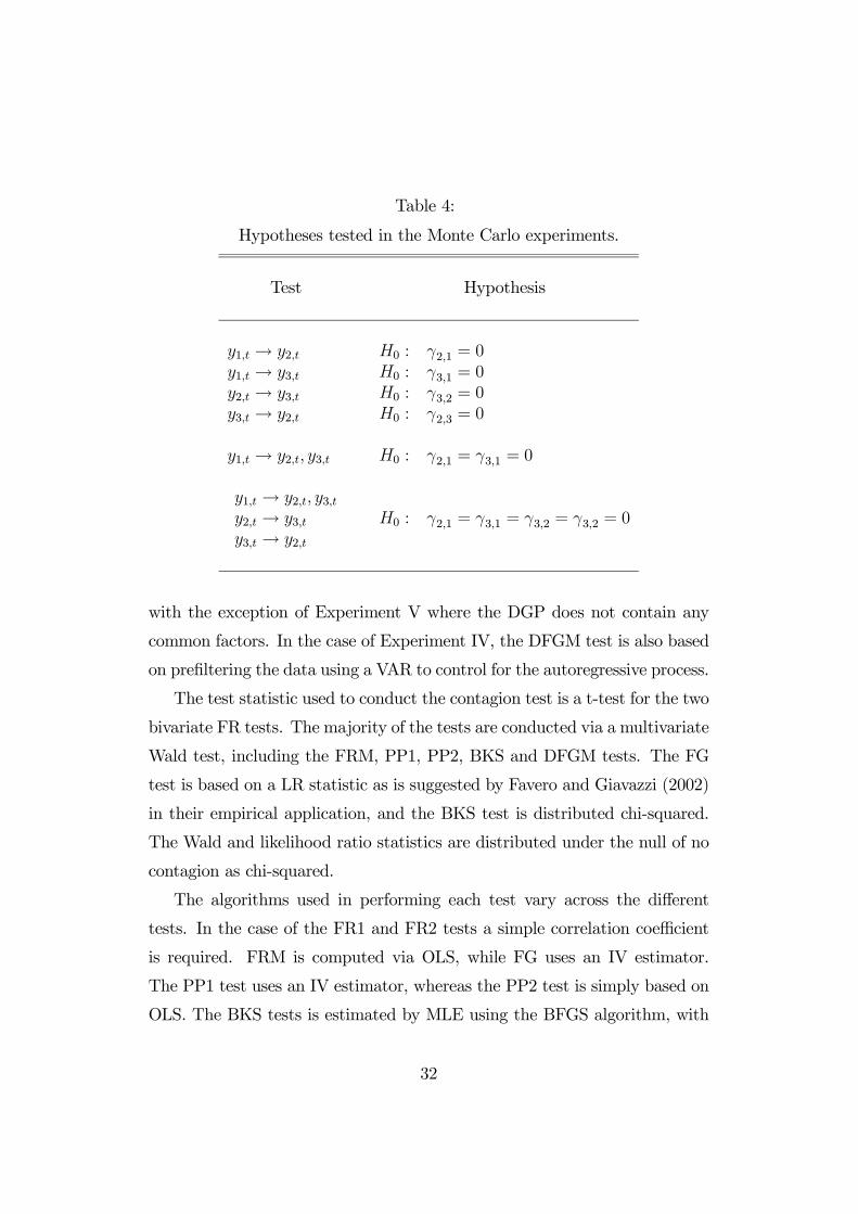
Table 4:

Hypotheses tested in the Monte Carlo experiments.

Test Hypothesis

y1,t → y2,t H0 : γ2,1 = 0y1,t → y3,t H0 : γ3,1 = 0y2,t → y3,t H0 : γ3,2 = 0y3,t → y2,t H0 : γ2,3 = 0

y1,t → y2,t, y3,t H0 : γ2,1 = γ3,1 = 0

y1,t → y2,t, y3,ty2,t → y3,ty3,t → y2,t

H0 : γ2,1 = γ3,1 = γ3,2 = γ3,2 = 0

with the exception of Experiment V where the DGP does not contain any

common factors. In the case of Experiment IV, the DFGM test is also based

on prefiltering the data using a VAR to control for the autoregressive process.

The test statistic used to conduct the contagion test is a t-test for the two

bivariate FR tests. The majority of the tests are conducted via a multivariate

Wald test, including the FRM, PP1, PP2, BKS and DFGM tests. The FG

test is based on a LR statistic as is suggested by Favero and Giavazzi (2002)

in their empirical application, and the BKS test is distributed chi-squared.

The Wald and likelihood ratio statistics are distributed under the null of no

contagion as chi-squared.

The algorithms used in performing each test vary across the different

tests. In the case of the FR1 and FR2 tests a simple correlation coefficient

is required. FRM is computed via OLS, while FG uses an IV estimator.

The PP1 test uses an IV estimator, whereas the PP2 test is simply based on

OLS. The BKS tests is estimated by MLE using the BFGS algorithm, with

32

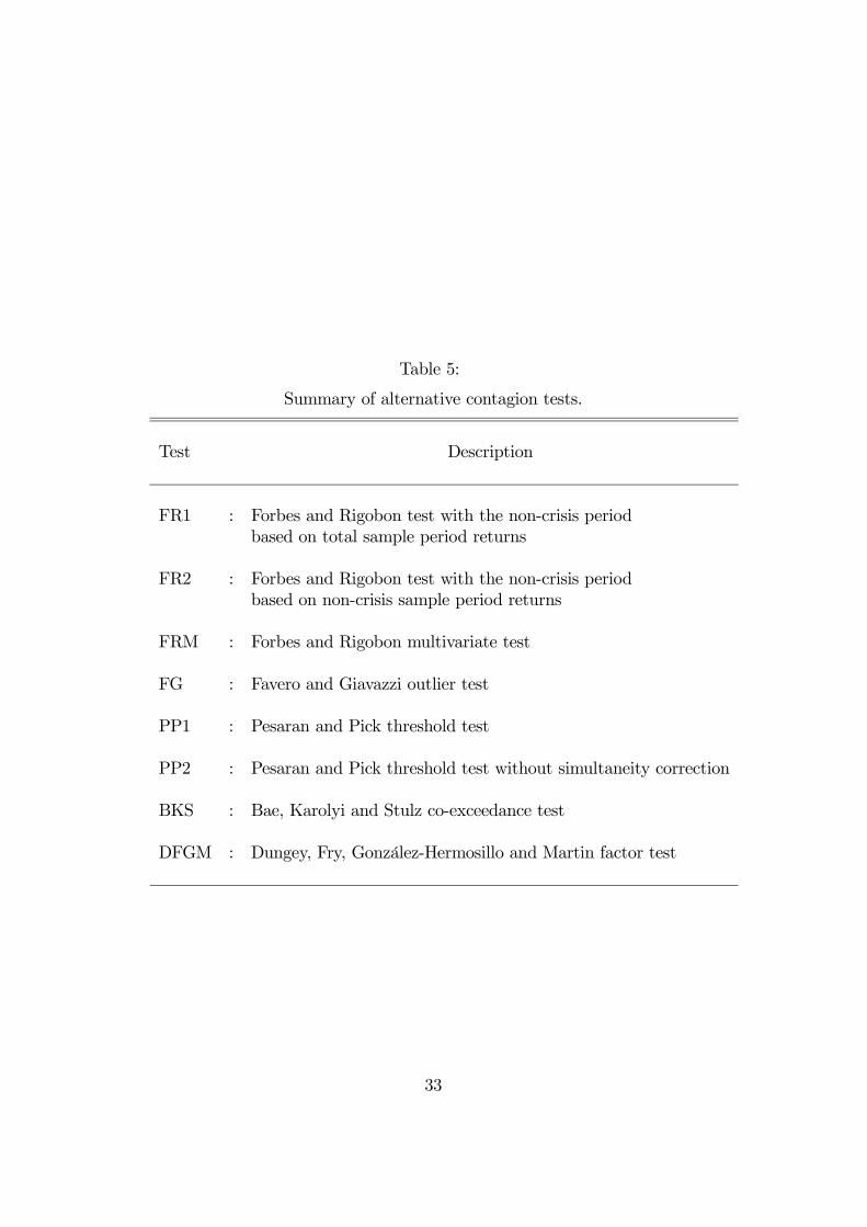
Table 5:

Summary of alternative contagion tests.

Test Description

FR1 : Forbes and Rigobon test with the non-crisis periodbased on total sample period returns

FR2 : Forbes and Rigobon test with the non-crisis periodbased on non-crisis sample period returns

FRM : Forbes and Rigobon multivariate test

FG : Favero and Giavazzi outlier test

PP1 : Pesaran and Pick threshold test

PP2 : Pesaran and Pick threshold test without simultaneity correction

BKS : Bae, Karolyi and Stulz co-exceedance test

DFGM : Dungey, Fry, González-Hermosillo and Martin factor test

33

the maximum number of iterations set at 200. The DFGM estimates are

carried out by GMM, estimated with MLE using the BFGS algorithm, with

a maximum number of 100 iterations and a maximum gradient tolerance

of 0.0001. The optimal weighting matrix is based on an adjustment for

heteroskedasticity, but no autocorrelation. Each Monte Carlo experiment

is conducted in Gauss 5.0, with the exception of PP1 and PP2 which are

undertaken in Gauss 6.0. The experiments are based on 10, 000 replications.

The normal random numbers are generated using the GAUSS procedure

RNDN, with a seed equal to 123457. The sample size is Tx = 100 for the

noncrisis period and Ty = 50 for the crisis period.

Each test was conducted across the range of five experiments outlined

in Table 3. For Experiments I, II and IV, the DFGM test is based on the

model specified in Section 4.8. In Experiment III, the common factor stru-

cural break is replaced by an idiosyncratic structural break, thereby leaving

the model with 12 moment conditions and 11 unknown parameters. For Ex-

periment V, the model is estimated without the common factor and hence

no structural break in the common factor.

5.3 Size

The finite sample results of the size of the eight contagion tests for each of

the five hypotheses, are presented in Table 6 (Experiments I, II and III) and

Table 7 (Experiments IV and V). The sizes are based on the 5% asymptotic

(chi-squared) critical values of the test statistics.

The FR1 test is consistently undersized (less than 0.050) for all experi-

ments with the test not rejecting the null of contagion often enough. This

bias towards failing to find contagion is consistent with much of the empirical

evidence where little evidence of contagion is detected using this test.

In contrast to the FR1 test, the FR2 test has good size properties for

a range of experiments and hypotheses. Some exceptions are in testing the

34

third and fourth hypotheses in Experiments II and IV (sizes in excess of

0.700) and the first two hypotheses in Experiment II (sizes of 0.000). The

good size properties of FR2 reflect that the independence assumption under-

lying the calculation of the variance of the FR1 test statistic are violated.

The FR1 test is based on the noncrisis period being the total sample period,

which is clearly correlated with the crisis period. This is not the case with

the FR2 test, where the noncrisis and crisis periods do not overlap. The two

experiments where the size of the FR2 test are inflated occur when there

is a structural break in the common factor. This suggests that this test is

not robust to this type of structural break. In the case of an idiosyncratic

structural break (Experiment III), the robustness results are mixed with the

test being correctly sized for the third and fourth hypotheses, but undersized

for the first and second hypotheses.

The FRM test also demonstrates good size properties for a range of ex-

periments and hypotheses tested. In general the size of this test is slightly

inflated compared to the size of FR2, which reflects that there is a loss of

efficiency in conducting the FRM test as a result of the additional parameters

that need to be estimated which are redundant under the null of no conta-

gion. In contrast to the FR2 test, the FRM test appears to be relatively

robust to a break in the common factor (Experiment II) with reasonable

sizes of between 0.086 and 0.180. However, this test is not robust to idiosyn-

cratic structural breaks (Experiment III) with sizes in excess of 0.166 for the

third and fourth hypotheses and in excess of 0.730 for the first and second

hypotheses.

The FG test appears to be consistently oversized for all experiments and

across all hypotheses tested. The test does not produce a size less than

0.200, with some sizes in excess of 0.700. This result is consistent with the

empirical applications of this test which tend to find strong evidence of con-

tagion (Favero and Giavazzi (2002), Billio and Pelizzen (2003)). The wide

dispersion of the sampling distribution of this test statistic reflects the weak

35

instrument problem in implementing the test. Comparing the size of the test

in Experiments II and IV shows that the size of the test improves slightly for

the latter experiment (ie closer to the nominal level of 0.05). This reflects

that the lagged returns now act as better instruments to correct for the si-

multaneity bias. However, even in this case the inflated sizes still suggest

that the instruments are weak.

The PP1 test is undersized in all experiments, while the PP2 test has em-

pirical sizes close to the nominal size of 0.05, for Experiments III and V, and

to a lesser extent Experiment I. This suggests that the PP1 test is affected by

weak instrument problems and that the order of the bias from not correcting

the simultaneity bias is of a lower order of magnitude that the bias incurred

from using weak instruments. The inflated sizes of PP2 in Experiment II

shows that this test is not robust to structural breaks in the common factor.

In contrast, the good size properties revealed in Experiment III, shows that

the test is potentially robust to structural breaks in the idiosyncratic factor.

The BKS test tends to be oversized for most experiments, especially when

there is a structural break in the common factor (Experiments II and IV).

The exception is Experiment V, where the sizes are marginally undersized

for the four single hypotheses. These results imply that the properties of the

test are affected by the way the common factor is modelled and the loss of

of information arising from the filters used to identify outliers.

The DFGM factor test performs relatively well across the five experiments

with just moderately inflated sizes. The worst cases are in Experiment III

where the sizes are around 0.2 for the single hypotheses.

5.4 Power

Tables 8 to 12 give the probability of finding contagion for each of the eight

tests for increasing intensity levels of contagion, δ = 1, 2, 5, 10, across the five

experiments. As contagion is assumed to run from y1,t to both y2,t and y3,t

36

during the crisis period, the power of the test should increase monotonically

as δ increases for the first two hypotheses, y1,t → y2,t and y1,t → y3,t. For the

third and fourth hypotheses, y2,t → y3,t and y3,t → y2,t, the power should be

equal to the size adjusted value of the test, namely 0.05.

5.4.1 Experiment 1: No structural breaks

Table 8 shows that the DFGM test has the highest power of all eight tests,

with powers monotonically increasing for the first two hypotheses to just over

0.95 for the maximum level of contagion (δ = 10). Both FR1 and FR2 have

low power, with the power at no stage being greater than 0.5. In both cases

the power functions are not monotonic, with the power for FR2 falling as

low as 0.089 for δ = 10, in the second hypothesis.

The FR2, FRM and BKS tests identify spurious contagion between y2,t

and y3,t, with the probability increasing to 1.0 for the third and fourth hy-

potheses in the case of FRM. The PP2 and DFGM tests tend to have inflated

probabilities with respect to these two hypotheses, whilst the PP1 test and

to a lesser extent the FG test, are correctly sized with probabilities near 0.05.

5.4.2 Experiment 2: Structural break in the common factor

Table 9 shows that the FRM and DFGM tests have good power properties

in detecting contagion in the presence of a structural break in the common

factor (first and second hypotheses). However, the FRM test incorrectly

identifies contagion between y2,t and y3,t, with the probabilities of detecting

contagion between these two variables increasing to 1.000 for δ = 10 (third

and fourth hypotheses).

The FR1 and FR2 tests show that these two tests are biased with the

power falling below 0.05. The BKS and PP2 tests also appear to be biased.

The power function of the PP1 test is montonically increasing, albeit at a

very slow rate.

37

5.4.3 Experiment 3: Structural break in the idiosyncratic factor

For the case of a structural break in the idiosyncratic factor of y1,t, Table

10 shows that the FR1 and FR2 tests, as well as the DFGM test, have very

steep power functions for the first two hypotheses with the power hitting 1.0

for all values of δ > 0. However, the FR2 test incorrectly detects contagion

between y2,t and y3,t (third and fourth hypotheses). The DFGM performs

better in that the probabilities of detecting contagion between y2,t and y3,t

are generally smaller than they are for the FR2 test.

The FRM performs badly on all accounts as it fails to find contagion when

it exists (first and second hypotheses), and finds contagion when it should

not (third and fourth hypotheses).

The FG, PP1, PP2 and BKS tests, all exhibit low powers. As all of these

tests are based on filtering methods to identify contagion, it would appear

that the filters result in a serious loss of information resulting in low powers.

5.4.4 Experiment 4: Autoregressive

A comparison of Tables 8 and 11, show that the introduction of autocorre-

lation into the DGP does not change the relative performance of the various

tests. The results do show a slight improvment in the power properties of

the FG and PP1 tests, which reflects that the the lagged returns now pro-

vide better instruments. However, as the improvement in power is marginal,

this also suggests that the instruments in this setting still nonetheless repre-

sent weak instruments, which result in finite sampling distributions deviating

significantly from the asymptotic distributions.

5.4.5 Experiment 5: No common factor

The results of Experiment V in Table 12 are very similar to the results of

Experiment III in Table 10. Namely, the tests that are not based on filtering

methods, FR1, FR2, FRM and DFGM, all exhibit very high powers for all

38

levels of contagion in the case of the first two hypotheses. In contrast, the

remaining four tests, FG, PP1, PP2 and BKS, all exhibit low powers. Of the

non-filtering set of contagion tests, the FR2 test detects spurious contagion

(hypotheses three and four) whereas the other three tests yield probabilities

close to the correct level of 0.05.

6 Conclusions

This paper has investigated the finite sample properties of a range of tests

of contagion commonly employed to detect propagation mechanisms during

financial crises. The tests investigated included the Forbes and Rigobon

adjusted correlation test, the Favero and Giavazzi outlier test, the Pesaran

and Pick threshold test, the Bae, Karolyi and Stulz co-exceedance test, and

the Dungey, Fry, González-Hermosillo and Martin GMM factor model test.

An important feature of the Monte Carlo experiments was an allowance for

increased volatility of the market fundamentals during financial crises as

well as contagion. The latter channel was modelled by allowing for shocks

in the returns of one country to impact on the returns of another country

during the crisis period. Five experiments were conducted involving testing

for contagion in the absence and presence of a common factor, in the absence

and presence of a structural break in the common factor, and in the absence

and presence of a structural break in the idiosyncratic factor. In addition,

the effect of autocorrelation in the common factor on the test outcomes was

also investigated.

The key results showed that the Favero and Giavazzi and the Bae, Karolyi

and Stulz tests were oversized and had low power, particularly in the pres-

ence of structural breaks. That is, these tests were biased towards find-

ing contagion. The Forbes and Rigobon test in its original form was un-

dersized, as were the tests of Pesaran and Pick, and both of these tests

again generally exhibited low power. The modified versions of the Forbes

39

and Rigobon tests showed better size properties, as did the Dungey, Fry,

González-Hermosillo and Martin test. The multivariate and modified bivari-

ate Forbes and Rigobon tests showed low power, although the multivariate

form of the test performed well in detecting contagion when there was no

common factor in the model. Overall the Dungey, Fry, González-Hermosillo

and Martin test performed the most satisfactorily, with good size properties

and reasonable power properties over the range of experiments undertaken.

This test also failed to detect spurious contagion channels unlike some of

the other tests, such as the multivariate Forbes and Rigobon test and the

co-exceedance test of Bae, Karolyi and Stulz.

In conclusion most of the current suite of tests for contagion tend to

exhibit poor size properties in the face of the typically small samples avail-

able, and in general low power. The tests are biased such that users of the

Forbes and Rigobon test in its original form or the Pesaran and Pick tests

are unlikely to find evidence of contagion when it does exist, while users of

the Favero and Giavazzi or Bae, Karolyi and Stulz tests are more likely to

find contagion when it does not exist. This suggests that users of these tests

should proceed with care in interpreting the results.

40

References

[1] Bae, K.H, Karolyi, G.A. and Stulz, R.M. (2003), “A New Approach

to Measuring Financial Contagion”, Review of Financial Studies, 16(3),

717-763.

[2] Baig, T. and Goldfajn, I. (1999), “Financial Market Contagion in the

Asian Crisis”, IMF Staff Papers, 46(2), 167-195.

[3] Baur, D. and Schulze, N. (2002), “Coexceedances in Financial Markets -

A Quantile Regression Analysis of Contagion”, University of Tuebingen

Discussion Paper 253.

[4] Bekaert, G., Harvey, C.R. and Ng, A. (2005), “Market Integration and

Contagion”, Journal of Business, 78(1), part 2, forthcoming.

[5] Billio, M. and Pelizzon, L. (2003), “Contagion and Interdependence in

Stock Markets: Have They Been Misdiagnosed?”, Journal of Economics

and Business, 55 405-426.

[6] Corsetti, G., Pericoli, M. and Sbracia, M. (2002), “Some Contagion,

Some Interdependence’: More Pitfalls in Testing for Contagion”, mimeo

University of Rome III.

[7] Dornbusch, R., Park, Y.C. and Claessens, S. (2000), “Contagion: Under-

standing How It Spreads”, The World Bank Research Observer, 15(2),

177-97.

[8] Dungey, M., Fry, R., González-Hermisillo, B. and Martin, V.L. (2002),

“The Transmission of Contagion in Developed and Developing Interna-

tional Bond Markets”, in Committee on the Global Financial System

(ed), Risk Measurement and Systemic Risk, Proceedings of the Third

Joint Central Bank Research Conference, 61-74 .

41

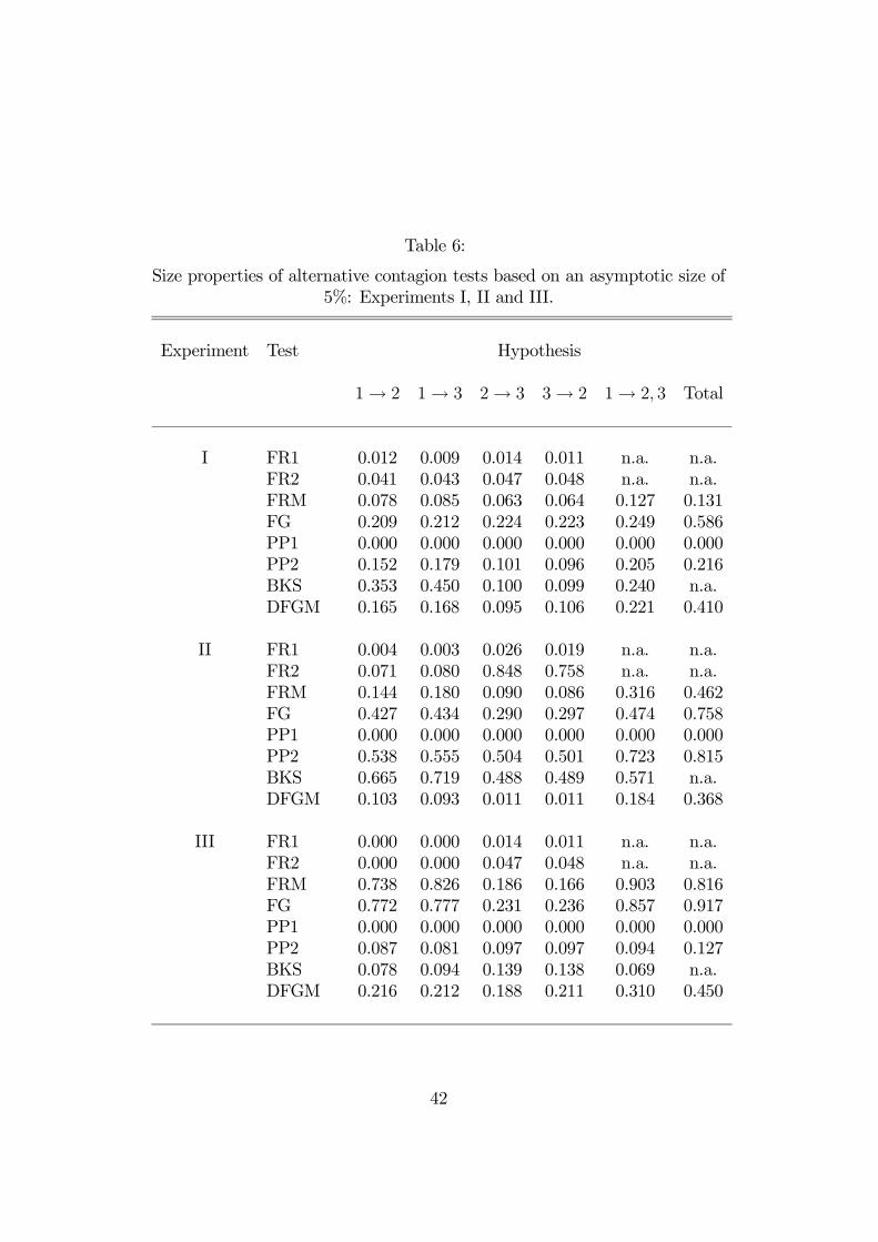
Table 6:

Size properties of alternative contagion tests based on an asymptotic size of5%: Experiments I, II and III.

Experiment Test Hypothesis

1→ 2 1→ 3 2→ 3 3→ 2 1→ 2, 3 Total

I FR1 0.012 0.009 0.014 0.011 n.a. n.a.FR2 0.041 0.043 0.047 0.048 n.a. n.a.FRM 0.078 0.085 0.063 0.064 0.127 0.131FG 0.209 0.212 0.224 0.223 0.249 0.586PP1 0.000 0.000 0.000 0.000 0.000 0.000PP2 0.152 0.179 0.101 0.096 0.205 0.216BKS 0.353 0.450 0.100 0.099 0.240 n.a.DFGM 0.165 0.168 0.095 0.106 0.221 0.410

II FR1 0.004 0.003 0.026 0.019 n.a. n.a.FR2 0.071 0.080 0.848 0.758 n.a. n.a.FRM 0.144 0.180 0.090 0.086 0.316 0.462FG 0.427 0.434 0.290 0.297 0.474 0.758PP1 0.000 0.000 0.000 0.000 0.000 0.000PP2 0.538 0.555 0.504 0.501 0.723 0.815BKS 0.665 0.719 0.488 0.489 0.571 n.a.DFGM 0.103 0.093 0.011 0.011 0.184 0.368

III FR1 0.000 0.000 0.014 0.011 n.a. n.a.FR2 0.000 0.000 0.047 0.048 n.a. n.a.FRM 0.738 0.826 0.186 0.166 0.903 0.816FG 0.772 0.777 0.231 0.236 0.857 0.917PP1 0.000 0.000 0.000 0.000 0.000 0.000PP2 0.087 0.081 0.097 0.097 0.094 0.127BKS 0.078 0.094 0.139 0.138 0.069 n.a.DFGM 0.216 0.212 0.188 0.211 0.310 0.450

42

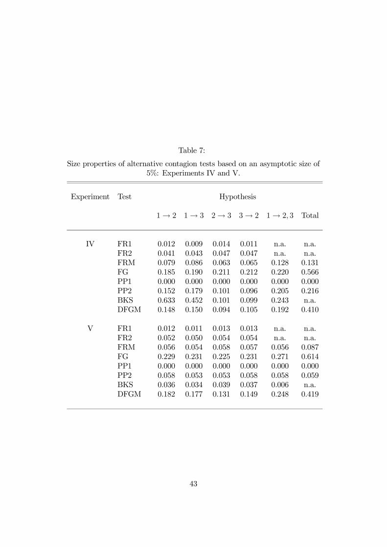
Table 7:

Size properties of alternative contagion tests based on an asymptotic size of5%: Experiments IV and V.

Experiment Test Hypothesis

1→ 2 1→ 3 2→ 3 3→ 2 1→ 2, 3 Total

IV FR1 0.012 0.009 0.014 0.011 n.a. n.a.FR2 0.041 0.043 0.047 0.047 n.a. n.a.FRM 0.079 0.086 0.063 0.065 0.128 0.131FG 0.185 0.190 0.211 0.212 0.220 0.566PP1 0.000 0.000 0.000 0.000 0.000 0.000PP2 0.152 0.179 0.101 0.096 0.205 0.216BKS 0.633 0.452 0.101 0.099 0.243 n.a.DFGM 0.148 0.150 0.094 0.105 0.192 0.410

V FR1 0.012 0.011 0.013 0.013 n.a. n.a.FR2 0.052 0.050 0.054 0.054 n.a. n.a.FRM 0.056 0.054 0.058 0.057 0.056 0.087FG 0.229 0.231 0.225 0.231 0.271 0.614PP1 0.000 0.000 0.000 0.000 0.000 0.000PP2 0.058 0.053 0.053 0.058 0.058 0.059BKS 0.036 0.034 0.039 0.037 0.006 n.a.DFGM 0.182 0.177 0.131 0.149 0.248 0.419

43

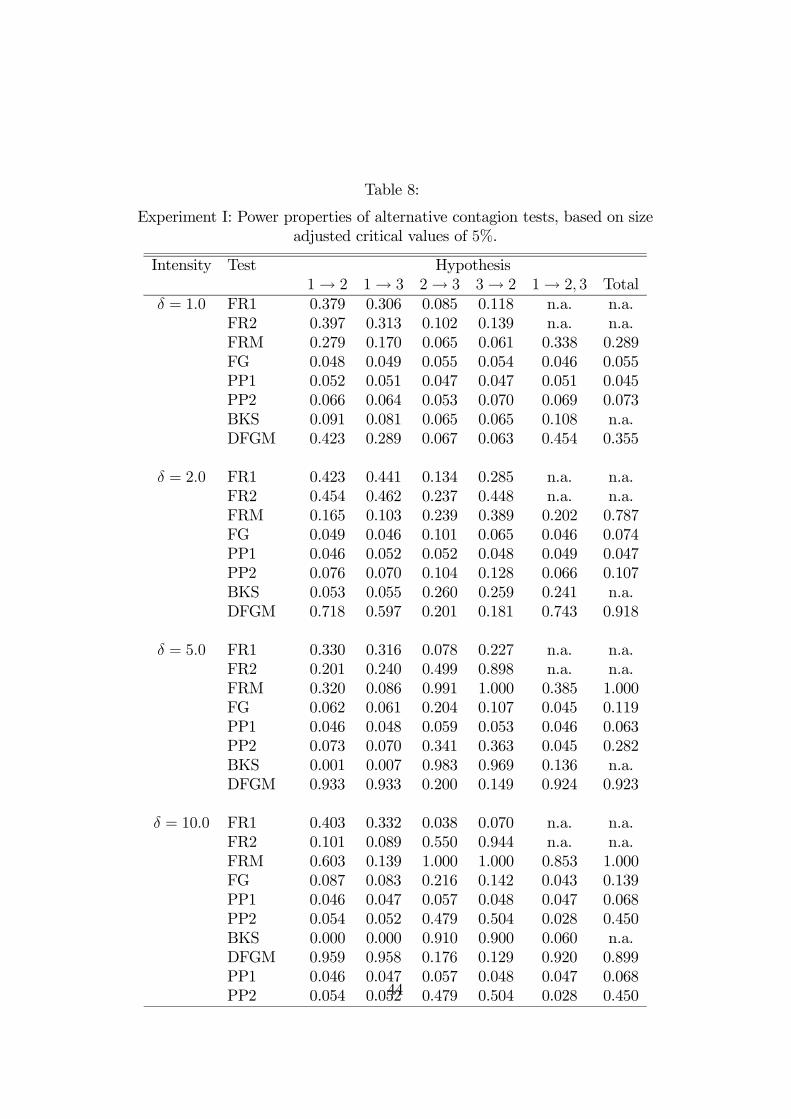
Table 8:

Experiment I: Power properties of alternative contagion tests, based on sizeadjusted critical values of 5%.

Intensity Test Hypothesis1→ 2 1→ 3 2→ 3 3→ 2 1→ 2, 3 Total

δ = 1.0 FR1 0.379 0.306 0.085 0.118 n.a. n.a.FR2 0.397 0.313 0.102 0.139 n.a. n.a.FRM 0.279 0.170 0.065 0.061 0.338 0.289FG 0.048 0.049 0.055 0.054 0.046 0.055PP1 0.052 0.051 0.047 0.047 0.051 0.045PP2 0.066 0.064 0.053 0.070 0.069 0.073BKS 0.091 0.081 0.065 0.065 0.108 n.a.DFGM 0.423 0.289 0.067 0.063 0.454 0.355



δ = 10.0 FR1 0.403 0.332 0.038 0.070 n.a. n.a.FR2 0.101 0.089 0.550 0.944 n.a. n.a.FRM 0.603 0.139 1.000 1.000 0.853 1.000FG 0.087 0.083 0.216 0.142 0.043 0.139PP1 0.046 0.047 0.057 0.048 0.047 0.068PP2 0.054 0.052 0.479 0.504 0.028 0.450BKS 0.000 0.000 0.910 0.900 0.060 n.a.DFGM 0.959 0.958 0.176 0.129 0.920 0.899PP1 0.046 0.047 0.057 0.048 0.047 0.068PP2 0.054 0.052 0.479 0.504 0.028 0.45044

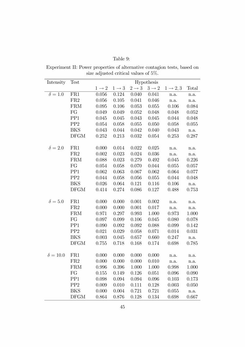
Table 9:

Experiment II: Power properties of alternative contagion tests, based onsize adjusted critical values of 5%.






45

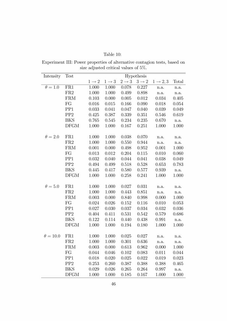
Table 10:

Experiment III: Power properties of alternative contagion tests, based onsize adjusted critical values of 5%.


θ = 1.0 FR1 1.000 1.000 0.078 0.227 n.a. n.a.FR2 1.000 1.000 0.499 0.898 n.a. n.a.FRM 0.103 0.000 0.005 0.012 0.034 0.405FG 0.016 0.015 0.166 0.090 0.018 0.054PP1 0.033 0.041 0.047 0.040 0.039 0.049PP2 0.425 0.387 0.339 0.351 0.546 0.619BKS 0.765 0.545 0.234 0.235 0.670 n.a.DFGM 1.000 1.000 0.167 0.251 1.000 1.000




46

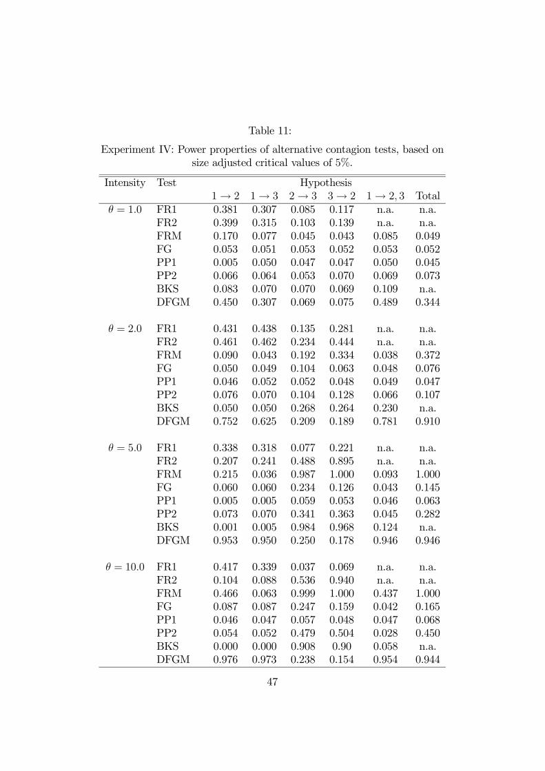
Table 11:

Experiment IV: Power properties of alternative contagion tests, based onsize adjusted critical values of 5%.






47

Table 12:

Experiment V: Power properties of alternative contagion tests, based onsize adjusted critical values of 5%.






48

[9] Dungey, M., Fry, R., González-Hermosillo, B. and Martin, V.L. (2004),

“A Comparison of Alternative Tests of Contagion with Applications”, in

M. Dungey and D. Tambakis (eds) International Financial Contagion:

A Reader, Oxford University Press, forthcoming.

[10] Dungey, M. and Martin, V.L. (2004), “AMultifactor Model of Exchange

Rates with Unanticipated Shocks: Measuring Contagion in the East

Asian Currency Crisis”, Journal of Emerging Markets Finance, 3, 305-

330.

[11] Dungey, M., Martin, V.L. and Pagan, A.R. (2000), “A Multivariate La-

tent Factor Decomposition of International Bond Yield Spreads”, Jour-

nal of Applied Econometrics, 15, 697-715.

[12] Eichengreen, B., Rose, A.K. and Wyplosz, C. (1995), “Exchange Mar-

ket Mayhem: The Antecedents and Aftermath of Speculative Attacks”,

Economic Policy, 21, 249-312.

[13] Eichengreen, B., Rose, A.K. and Wyplosz, C. (1996), “Contagious Cur-

rency Crises”, NBER Working Paper, 5681.

[14] Favero, C.A. and Giavazzi, F. (2002), “Is the International Propagation

of Financial Shocks Non-linear? Evidence from the ERM”, Journal of

International Economics, 57 (1), 231-46.

[15] Forbes, K. and Rigobon, R. (2002), “No Contagion, only Interdepen-

dence: Measuring Stock Market Co-movements”, Journal of Finance,

57 (5), 2223-61.

[16] Glick, R. and Rose, A.K. (1999), “Contagion and Trade: Why are Cur-

rency Crises Regional?”, Journal of International Money and Finance,

18(4), 603-17.

49

[17] Kaminsky, G.L. and Reinhart, C.M. (2000), “On Crises, Contagion and

Confusion”, Journal of International Economics, 51(1), 145-168.

[18] Kaminsky, G.L. and Reinhart, C.M. (2001), “Financial Markets in

Times of Stress”, NBER Working Paper, 8569.

[19] Loretan, M. and English, W. (2000), “Evaluating "Correlation Break-

downs" During Periods of Market Volatility”, Board of Governors of the

Federal Reserve System, International Finance Discussion Paper No.

658.

[20] Lowell, J., Neu, C.R. and Tong, D. (1998), “Financial Crises and Con-

tagion in Emerging Market Countries”, Monograph, RAND.

[21] Mody, A, and Taylor, M.P. (2003), “Common Vulnerabilities”, CEPR

Discussion Paper 3759.

[22] Pesaran, H. and Pick, A. (2003), “Econometric Issues in the Analysis of

Contagion”, CESifo Working Paper 1176.

[23] Pericoli, M. and Sbracia, M. (2003), “A Primer on Financial Contagion”,

Journal of Economic Surveys, 17(4), 571-608.

[24] Pritsker, M. (2002), “Large Investors and Liquidity: A Review of the

Literature”, in Committee on the Global Financial System (ed), Risk

Measurement and Systemic Risk, Proceedings of the Third Joint Central

Bank Research Conference.

[25] Rigobon, R. (2003), “On the Measurement of the International Propoga-

tion of Shocks: Is the Transmission Stable?”, Journal of International

Economics, 61, 261-283.

[26] Walti, S. (2003), “Testing for Contagion in International Financial mar-

kets: WhichWay to Go?”, The Graduate Institute of International Stud-

ies, Geneva, HEI Working Paper No: 04/2003.

50

Documents

A Monte Carlo Analysis of Alternative Tests of … · A Monte Carlo Analysis of Alternative Tests of Contagion ... ity model test, and the Dungey, Fry, González-Hermosillo and Martin