A Modular Genetic Algorithm for Scheduling Task Graphs

Michael Rinehart, Vida Kianzad, and Shuvra S. BhattacharyyaDepartment of Electrical and Computer Engineering, and

Institute for Advanced Computer StudiesUniversity of Maryland, College Park, MD 20742

{mdrine, vida, ssb}@eng.umd.edu

Abstract. Several genetic algorithms have been designed for the problem of scheduling task

graphs onto multiprocessors, the primary distinction among most of them being the chromosomal

representation used for a schedule. However, these existing approaches are monolithic as they

attempt to scan the entire solution space without consideration to techniques that can reduce the

complexity of the optimization. In this paper, a genetic algorithm based in a bi-chromosomal rep-

resetnation and capable of being incorporated into a cluster/merging optimization framework is

proposed, and it is experimentally shown to outperform a leading genetic algorithm for schedul-

ing.

Keywords: Evolutionary computing and genetic algorithms, scheduling and task partitioning,

graph algorithms.

1. IntroductionThe problem of scheduling task graphs onto multiprocessors is a well-defined problem

that has received a large amount of attention in the literature. This problem involves mapping an

acyclic directed graph, which describes a collection of computational tasks and their data prece-

dences, onto a parallel processing system. Many of the techniques for this problem, such as those

described in [5, 8, 9, 12], have been developed with moderate complexity as a constraint, which is

a reasonable assumption for general purpose development platforms. More recently, however,

with the increasing availability of computing power, and the increasing importance of embedded

systems, in which compile-time tolerances are significantly higher than in general purpose

domains (e.g., see [6]), genetic algorithms have received significant interest in solving the multi-

1

processor scheduling problem.

Genetic algorithms are a form of probabilistic search that trades off increased computa-

tional requirements for the potential to achieve more extensive coverage of the search space.

Genetic algorithms mimic the process of natural evolution by maintaining at each step a popula-

tion of chromosomes (candidate solutions), and iteratively changing the population by applying

operators such as crossover (the combination of a pair of chromosomes to generate a new chro-

mosome) and mutation (the random perturbation of an existing chromosome). A fitness function,

which measures the quality of each candidate solution according to the given optimization objec-

tive, is used to help determine which chromosomes are retained in the population as successive

generations evolve [1].

In this paper, we introduce a new type of genetic algorithm for the multiprocessor schedul-

ing problem, one that uses a clustering/merging framework for reducing the complexity of the

search. Existing genetic algorithms either do not or cannot easily apply such a modular frame-

work, the latter condition being a consequence of a solution representation that entirely encodes a

schedule in a single data structure. The ability for our approach to sort clusters, rather than just

tasks, without the generation of invalid solutions or added complexity stems from the use of a new

type of chromosomal representation, the bi-chromosome. Encoding task assignment and execu-

tion order in two independent structures, the bi-chromosome allows new solutions to be generated

fairly easily and without loss in expressiveness in the solution space.

The paper is organized as follows. In section 3, a brief overview of the latest state-of-the-

art genetic algorithm for multiprocessor scheduling is presented, and its design advantages and

disadvantages are discussed. Our algorithm will be compared both in design and operation to this

benchmark approach.

In section 4, we introduce our genetic algorithm. The structure of the bi-chromosomal rep-

resentation, its relationship to an executable schedule, and the genetic operators that manipulate

realizations of this form are introduced. The details of the algorithm’s multi-phase layout are then

explained.

2

The results comparing the performance of our approach to the benchmark algorithm is

presented in section 5. We tested the two algorithms on three sets of graphs, allowing us to isolate

the performance of each algorithm in the realms of true application graphs, purely random graphs,

and graphs specifically varied to eliminate any bias resulting from a particular scheduling strat-

egy. Finally, we conclude the paper with some final remarks and potential avenues for future

research.

2. DefinitionsLet a task graph be a directed, acyclic graph composed of a set of vertices

, each vertex termed a task of the graph, and a set of edges where each edge is

denoted by an ordered pair of tasks . The set of predecessor and successor tasks of a task

are referred to by and respectively, and the transitive closure of is denoted

as .

Each task of the task graph represents an arbitrary process that requires a set of input data

in order execute. Before executing, a task waits for the completion of its predecessors’ executions,

using the output of its predecessors as the input for its own execution. Upon completion, the task

generates output data, which is then used by its successor tasks for their own execution. There is a

hierarchy in the order of execution of a task graph such that the execution of the graph must begin

with the root tasks and complete with the leaf tasks.

There are additional timing constraints placed upon task execution. The number of time

units required by a task to completely execute is called the delay of the task and is denoted as

. The number of time units required for data generated by a task to reach its succes-

sor task is called the interprocessor communication cost of edge and is denoted as

. So, for example, if task is determined to have started its execution at time , then

task must wait, depending upon the starting time of its other predecessor tasks, at least until

time before it can start executing.

A task graph may be mapped to a processor set in the manner of

each task of the task graph being assigned to exactly one processor. If two tasks are assigned to

G N

T t1 t2 … t, N, ,{ }=

t1 t2,( ) t

predG t( ) succG t( ) G

G+

t

delayG t( ) ti

tj ti tj,( )

ipcG ti tj,( ) ti x

tj

x delayG ti( ) ipcG ti tj,( )+ +

P p1 p2 … pM, , ,{ }=

3

the same processor, then the interprocessor communication cost of the edge connecting them, if

such an edge exists, is . Furthermore, no two tasks assigned to the same processor can execute

simultaneously.

A set of processor assignments and execution timings for the individual tasks of a task

graph is called a schedule. Given a schedule , the processor to which a task is assigned is

denoted as , and its starting time and finishing time is referred to by and

respectively. The total time required by a schedule to completely execute is called the

schedule’s makespan, and it is defined as .

The goal of the multiprocessor scheduling problem is to minimize the makespan of a par-

ticular task graph by generating a set of task assignments and execution orderings.

3. Existing Genetic AlgorithmsSeveral genetic algorithms have been developed for multiprocessor task scheduling, the

primary distinction among them being the chromosomal representation of a schedule. The struc-

ture of and restrictions placed upon the chromosomal representation significantly impact the com-

plexity of the genetic operators as well as the algorithm’s potential for convergence to an optimal

schedule. For example, Wang and Korfhage [11] make use of a binary matrix encoding that

records the assignment and the execution order of the tasks on each processor. However, the rules

governing the form of a valid solution are not fully accounted for by the crossover and mutation

operators and, as a consequence, there is the potential for the production of inexecutable sched-

ules. Although repair operations are implemented to correct these solutions, the operations con-

sume time that could otherwise be dedicated purely to the optimization.

Hou, Ansari, and Ren [3] propose a very different representation. Variable-length strings,

rather than matrices of fixed dimensions, are used to explicitly list the order of the tasks on each

processor. Although the restrictions placed upon the string representation prevent the production

of invalid solutions, it is proven by Correa, Ferreira, and Rebreyend [2] that this representation

cannot express the full range of possible schedules. Hence, it may be impossible for the genetic

algorithm to converge to an optimal solution regardless of the amount of time allocated to the

0

S t

PS t( ) startS t( )

finishS t( )

makespan maxt T∈ finishS t( ){ }=

4

optimization.

Correa et al. improve upon the work by Hou et al. and propose the full-search genetic

algorithm (FSG), which uses a string representation capable of spanning the entire space of possi-

ble schedules. Although FSG significantly outperforms its predecessor, additional list-heuristics

that leverage some knowledge about the scheduling problem were added to FSG to further

improve the quality of its schedules. The culminating algorithm was termed the combined-genetic

list algorithm (CGL). CGL dramatically outperforms its predecessors, and, for this reason, it is

used in this paper to benchmark the quality of the bi-chromosomal genetic algorithm proposed in

section 4.

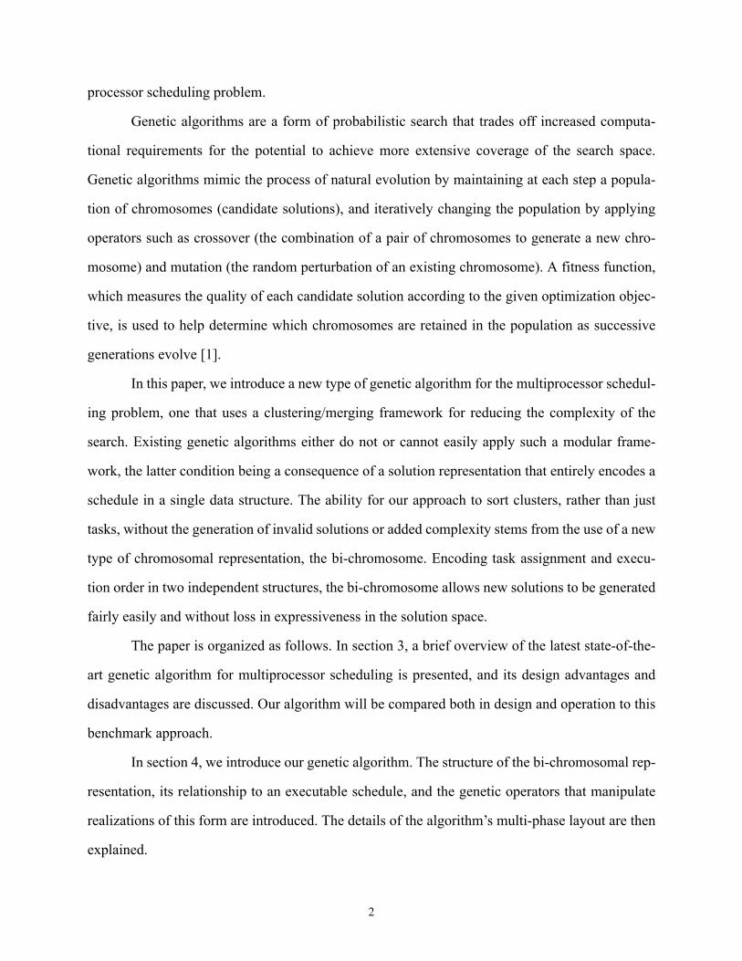
3.1. Chromosomal Representation as StringsSolutions in CGL are represented as list of strings, each string corresponding to one pro-

cessor of the target system. The strings maintain both the assignment and execution order of the

tasks on each processor. Figure 1 illustrates the relationship between an arbitrary schedule for an

task graph and its corresponding string representation in CGL.

More formally, given processors for a target system, each solution is encoded as a set of

strings where string corresponds to processor of the real system.

3.2. Knowledge-Augmented CrossoverFor two solutions and , the crossover operation first determines two partitions

and of the tasks in the graph such that the first partition contains all the predecessor tasks of

the latter partition. Information from the two parent solutions are included into these partitions in

1

2 3

4 5

6

7

StringRepresentation

Task Graph

Schedule

s1: 1-5-4

s3: 3-6-7s2: 2

p1:

p2:

p3: 3

1 5 4

6 72

timeFigure 1. Illustration of the string representation of a schedule

m

S s1 s2 … sm, , ,{ }= sj pj

S1 S2 V1

V2

5

the form of additional predecessor-successor relationships determined by those tasks that lie in the

same strings in each solution. The two partitions respectively represent the left and right portions

of the parent solutions.

Once the partitions are formed, the tasks from each must be placed into the new child solu-

tions. For the first child, the tasks from partition are placed exactly as they are assigned and

ordered in parent solution . For those tasks in partition , a list heuristic called earliest date/

most immediate successors first (ED/MISF) is used for selecting tasks from the partition and plac-

ing them into the child solution. Specifically, among those tasks equally satisfying the ED/MISF

requirement (determined by precedence constraints and by those tasks already scheduled), one is

randomly selected and placed onto the processor in the child solution where it has the earliest start

time. The second child is generated by the same algorithm with the roles of and inter-

changed.

3.3. Knowledge-Augmented MutationMutation in CGL is, in essence, a complete rearrangement of the tasks in a solution. Each

task is scheduled into a new solution according to a set of rules similar to that of the crossover

operator. Information about the original solution is incorporated in the form of additional prede-

cessor-successor relationships that affect how the tasks are selected for scheduling into the new

solution.

3.4. Drawbacks to CGLIt was empirically shown by Correa et al. that the heuristics incorporated within the cross-

over and mutation operators dramatically improve the performance of CGL relative to its prede-

cessor FSG. However, the authors note that a price in complexity is incurred. For example, each

instance of the crossover operator calls for numerous computations and comparisons for selecting

and placing individual tasks. A similar but lesser complexity is required by the mutation operator.

Although these heuristics introduce significant overhead into the genetic operators, there

exists an underlying complexity in both FSG and CGL that directly results from the use of a string

representation. In both algorithms, the crossover operator performs significant graph manipula-

V1

S1 V2

S1 S2

6

tions and requires the timely generation of partitions. The mutation operator resorts and reassigns

every task in the solution.

Furthermore, the solutions generated by the genetic operators do not generally resemble

the solutions from which they are derived, a direct consequence of the rigidity of the string repre-

sentation. Although it is desirable for the mutation operator to make small modifications to a solu-

tion, such as a task moving from one processor to another, it is necessary that schedule validity be

accounted for, and a check for this property with each task-shift may be more costly than a com-

plete reconstruction of the schedule. Crossing over two string representations has similar draw-

backs.

Finally, it should be noted that a string representation does not permit the use of a modular

optimization framework that incorporates clustering and merging techniques, and, therefore, the

potential for a reduction in algorithmic complexity that results from such a modular framework

cannot be leveraged. This is as an important part of the motivation behind our new scheduling

technique, called the bi-chromosomal genetic algorithm, which we introduce in the following sec-

tion.

4. Bi-Chromosomal Genetic AlgorithmThe Bi-Chromosomal Genetic Algorithm (BCGA) overcomes many of the complexities

inherent in monolithic searches, such as CGL, through its use of a solution representation that

divides the information content of the string representation into two, independent structures. As it

will be shown, this representation decreases the complexity of the genetic operators, and allows

for the use of an efficient, multiphase search.

4.1. BCGA’s Meta-OptimizationBCGA’s ability to sort clusters of tasks rather than just individual tasks allows it to be used

as a merging algorithm in a multiphase optimization, the implementation details for which is dis-

cussed in later sections. For now it suffices to note that BCGA is executed within the latter two

7

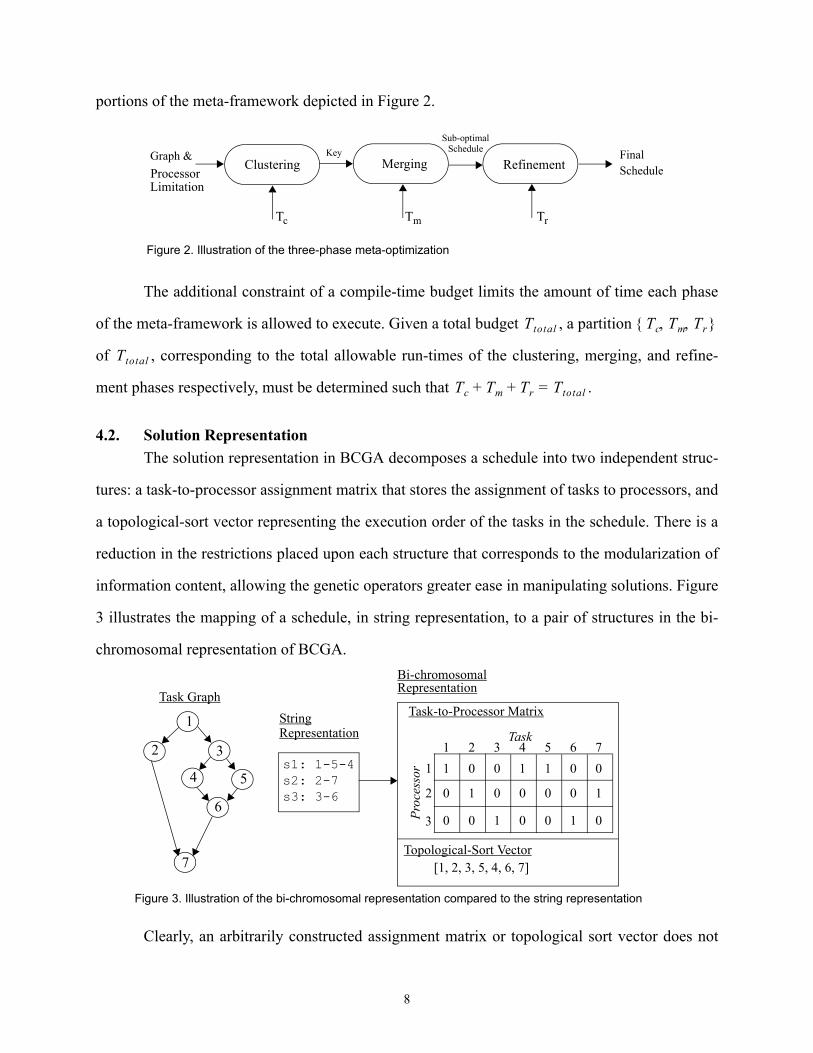
portions of the meta-framework depicted in Figure 2.

The additional constraint of a compile-time budget limits the amount of time each phase

of the meta-framework is allowed to execute. Given a total budget , a partition

of , corresponding to the total allowable run-times of the clustering, merging, and refine-

ment phases respectively, must be determined such that .

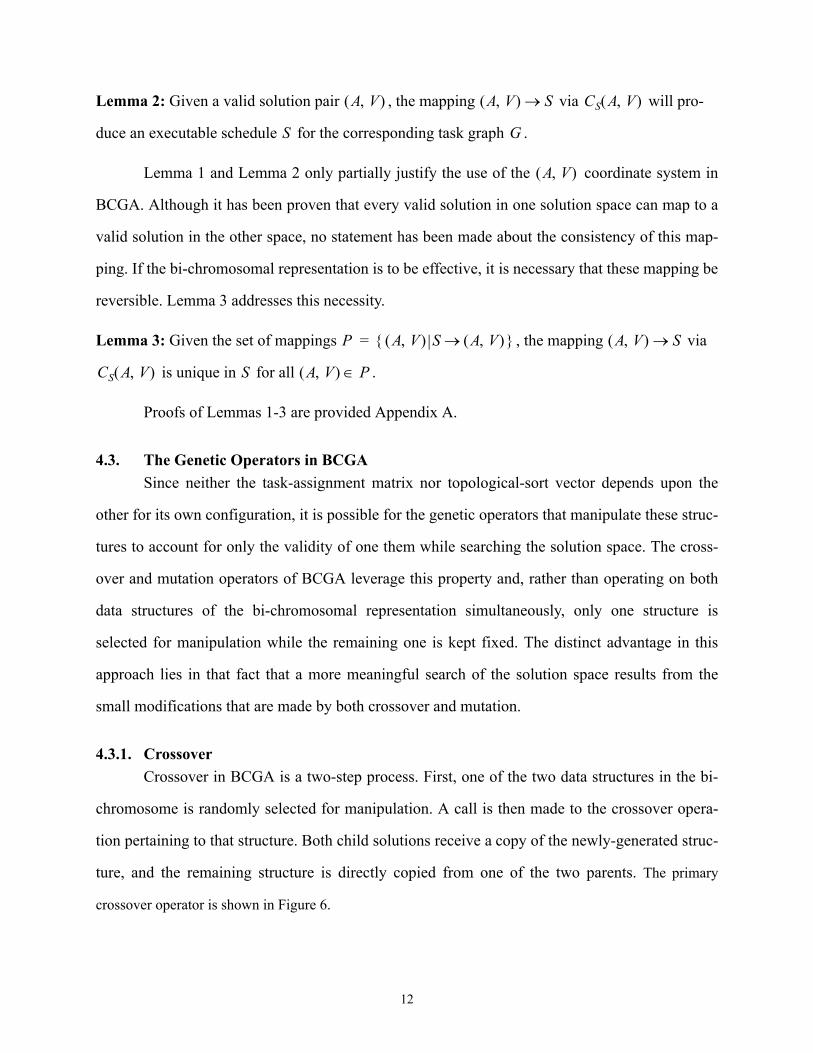
4.2. Solution RepresentationThe solution representation in BCGA decomposes a schedule into two independent struc-

tures: a task-to-processor assignment matrix that stores the assignment of tasks to processors, and

a topological-sort vector representing the execution order of the tasks in the schedule. There is a

reduction in the restrictions placed upon each structure that corresponds to the modularization of

information content, allowing the genetic operators greater ease in manipulating solutions. Figure

3 illustrates the mapping of a schedule, in string representation, to a pair of structures in the bi-

chromosomal representation of BCGA.

Clearly, an arbitrarily constructed assignment matrix or topological sort vector does not

Clustering Merging Refinement

Tc Tm Tr

ScheduleFinalGraph &

ProcessorLimitation

KeySub-optimal

Schedule

Figure 2. Illustration of the three-phase meta-optimization

Ttotal Tc Tm Tr, ,{ }

Ttotal

Tc Tm Tr Ttotal=+ +

1

2 3

4 5

6

7

s1: 1-5-4

s3: 3-6s2: 2-7

Topological-Sort Vector[1, 2, 3, 5, 4, 6, 7]

1 2 3 4 5 6 71

2

3Proc

esso

r

Task

0 1 0 0

1 0 0 0 0

0 0 1 0 0

1 0 1

0 1

0 1

Task-to-Processor MatrixStringRepresentation

Task Graph

Bi-chromosomalRepresentation

Figure 3. Illustration of the bi-chromosomal representation compared to the string representation

8

necessarily map to a valid schedule and, therefore, restrictions must be placed upon the individual

configurations of each structure. A configuration that satisfies such rules will be termed valid.

4.2.1. Proper Configuration and Interpretation of the Task-to-Processor Assignment Matrix

The task-to-processor assignment matrix represents, as the name suggests, the assignment

of tasks to processors for a particular schedule. Simply stated, if an element of an assignment

matrix has a value of 1, then task is assigned to processor in the corresponding schedule.

In general, an assignment matrix is valid if it satisfies the following two rules.

• Rule A1: is a binary matrix.

• Rule A2: Every column of possesses exactly one non-zero element. If an element

has a value of 1, then every other element of the same column, for , must be 0.

Therefore, the magnitude of each column, , is equal to 1 for all .

It should be noted that the restrictions placed upon the task-to-processor assignment

matrix allow it to be equivalently represented by a one-dimensional vector, where each index of

the vector corresponds to an individual task in the graph. However, since the data structure is rep-

resented as a matrix in the implementation of BCGA used in the experimental portion of this doc-

ument, the remainder of the paper concerns itself with the matrix representation. The algorithms

and proofs concerning the task-to-processor matrix can easily be translated for the equivalent

task-to-processor vector.

4.2.2. Proper Configuration and Interpretation of the Topological Sort VectorThe topological-sort vector explicitly represents the execution order of the tasks for a par-

ticular schedule. Such a vector is valid if it satisfies the following two rules.

• Rule V1: Every task of the given task graph appears exactly once in , and contains

no tasks other than those tasks from the graph.

• Rule V2: The order of the tasks in must satisfy a valid topological sorting of the given

graph . More formally, for all .

aij

A tj pi

A

aj A

aij aik i k≠

aj j

V

V V

V

G vk succG+ vj( )∉ 1 k j N≤<≤

9

4.2.3. Mapping a Schedule to a Solution Pair and Vice-VersaMapping a schedule to a solution pair is possible via the two algorithms

and . Specifically, . It should be noted that the ability to apply

two distinct algorithms for this mapping is a direct consequence of the independence between task

assignment and execution order in the solution representation employed by BCGA.

Simply put, the function , shown in Figure 4, duplicates the task-to-processor

assignments of the schedule into the matrix . For each task of the task graph, element is

set to if task is assigned to processor is the schedule or, in other words, .

The function , shown in Figure 5, does not produce such a simple, one-to-one rela-

tionship. The mapping of the execution order within a schedule, which may possess the parallel

execution of some tasks, onto a linear topological-sort vector, which is unable to depict anything

but linear execution, allows some tasks to be placed arbitrarily within the vector.

S A V,( ) CA S( )

CV S( ) A V,( ) CA S( ) CV S( ),( )=

CA S( )

S A t ait

1 t i S PS t( ) i=

1. function

2. Set to the zero matrix

3. // For each task t in the schedule S, assign the task to the appropriate

4. // processor in the assignment matrix.

5. for begin

6.

7.

8. end for

7. end function

A CA S( )=A

t 1…N=i PS t( )←

ait 1←

Figure 4. Pseudocode for CA()

CV S( )

10

The algorithm maintains a set of the tasks in the schedule that have not yet been

mapped into the vector . Among those tasks in with the earliest start times in , one is ran-

domly selected, placed into , and removed from . The algorithm repeats this process until

every task has been mapped.

The freedom of task selection implies that can generate several distinct vectors as

representations for the order-of-execution of the tasks in . Although the lack of a unique rela-

tionship between and results in somewhat redundant solution space, it is easily compensated

by the overall solution space reduction resulting from a clustering/merging framework.

Lemma 1: Given an executable schedule , the mapping via and pro-

duces a valid and a valid .

The mapping of a solution pair to a schedule is achieved via the function . The

function scans linearly through the topological-sort vector and, for each task selected from the

vector, it assigns the task to the appropriate processor and computes its starting time as a function

of its predecessors and by those tasks previously scheduled on the same processor.

1. function

2.

3. // Assign a task to each index j in the vector V.

4. for begin

5. // Determine the tasks with the earliest start times in S.

6.

7.

8. pick some

9. // Place the selected task into V and remove it from Tleft

10.

11.

12. end for

13. end function

V CV S( )=Tleft T←

j 1…N=

Xmin mint Tleft∈ startS t( ){ }←

T′ t{ Tleft startS t( )∈← Xmin}=t′ T′∈

vj t′←

Tleft Tleft t′{ }–←

Figure 5. Pseudocode for CV()

Tleft S

V Tleft S

V Tleft

Cv S( )

S

S V

S S A V,( )→ CA S( ) CV S( )

A V

CS A V,( )

11

Lemma 2: Given a valid solution pair , the mapping via will pro-

duce an executable schedule for the corresponding task graph .

Lemma 1 and Lemma 2 only partially justify the use of the coordinate system in

BCGA. Although it has been proven that every valid solution in one solution space can map to a

valid solution in the other space, no statement has been made about the consistency of this map-

ping. If the bi-chromosomal representation is to be effective, it is necessary that these mapping be

reversible. Lemma 3 addresses this necessity.

Lemma 3: Given the set of mappings , the mapping via

is unique in for all .

Proofs of Lemmas 1-3 are provided Appendix A.

4.3. The Genetic Operators in BCGASince neither the task-assignment matrix nor topological-sort vector depends upon the

other for its own configuration, it is possible for the genetic operators that manipulate these struc-

tures to account for only the validity of one them while searching the solution space. The cross-

over and mutation operators of BCGA leverage this property and, rather than operating on both

data structures of the bi-chromosomal representation simultaneously, only one structure is

selected for manipulation while the remaining one is kept fixed. The distinct advantage in this

approach lies in that fact that a more meaningful search of the solution space results from the

small modifications that are made by both crossover and mutation.

4.3.1. CrossoverCrossover in BCGA is a two-step process. First, one of the two data structures in the bi-

chromosome is randomly selected for manipulation. A call is then made to the crossover opera-

tion pertaining to that structure. Both child solutions receive a copy of the newly-generated struc-

ture, and the remaining structure is directly copied from one of the two parents. The primary

crossover operator is shown in Figure 6.

A V,( ) A V,( ) S→ CS A V,( )

S G

A V,( )

P A V,( ) S A V,( )→{ }= A V,( ) S→

CS A V,( ) S A V,( ) P∈

12

4.3.1.1.Matrix CrossoverThe simplicity of the task-to-processor assignment matrix translates into a reasonably sim-

ple crossover operation. As depicted in Figure 7, the left and right portions of each matrix, deter-

mined by a random cutoff point, are simply cropped from the parent solutions and interchanged

for the child solution. The formal algorithm is presented in Figure 8.

1.function

2. // Randomly select one of the structures for crossover

3.

4. if then

5. // Crossover the assignment matrix. Each child solution

6. // receives a copy of the new matrix, and its vector from a parent.

7.

8.

9. else

10. // Crossover the sort vector. Each child solution receives a

11. // copy of the new vector, and its matrix from a parent.

12.

13.

14. end if

15. end function

Ac1 Vc1,( ) Ac2 Vc2,( ),{ } crossover Ap1 Vp1,( ) Ap2 Vp2,( ),( )=

p a random real number in the range [0,1]←

p 0.5<

Ac crossoverA Ap1 Ap2,( )←

Ac1 Vc1,( ) Ac2 Vc2,( ),{ } Ac Vp1,( ) Ac Vp2,( ),{ }←

Vc crossoverV V1 V2,( )←

Ac1 Vc1,( ) Ac2 Vc2,( ),{ } Ap1 Vc,( ) Ap2 Vc,( ),{ }←

Figure 6. Pseudocode for the main crossover operator

13

Lemma 4: The crossover of two valid parent matrices will generate a valid child matrix .

Proof: Because the columns of are set to the columns of either parent, and since the columns of

both these matrices individually satisfy Rule A1 and Rule A2, the columns of must also satisfy

the two rules and, therefore, is valid.

4.3.1.2.Vector CrossoverThere is an increased complexity in crossing over two topological-sort vectors since the

restrictions placed upon the vector prevents the use of a simple, swapping operation. Instead, a

topological sorting algorithm is used to mix both parent solutions into a child solution, the criteria

for selecting tasks in the sort being based upon the order of the tasks in the two parent vectors.

At each iteration, the algorithm must, from one of the two parents, determine the task to

select from the set of ready tasks for placement into the child solution. The vector , representing

one of the two parent vectors, is used for this determination. From the set of ready tasks, the task

with the earliest placement in is chosen and appended to the child vector. Before the algorithm

reiterates, the identity of switches to other parent vector, which is then used for the subsequent

task selection. A formal outline of the algorithm is presented in Figure 10. An example of the crossover

1 2 3 4 51

2

3

0 0

1 0 0 1

0 0 1 1

0 0 0

1

0

1 2 3 4 51

2

3

0 1

0 0 0 0

0 1 1 0

1 0 1

0

0

1 2 3 4 51

2

3

0 0

0 0 0 1

0 1 1 1

1 0 0

0

0

X =

Parent 1 Parent 2 Child

Figure 7. Illustration of matrix crossover

1. function

2.

3. for

4. for

5. end function

A crossoverA B C,( )=d a random integer in the range [2, N]←

Ai Bi← 1 i d<≤

Ai Ci← d i N≤ ≤

Figure 8. Pseudocode for crossoverA()

A

A

A

A

P

P

P

14

operator is depicted in Figure 9.

Lemma 5: The crossover of two valid topological sort vectors will generate a valid child vector

.

Parent 1Parent 2Child

[1, 3, 5, 4, 6, 2, 7][1, 3, 2, 4, 5, 6, 7][1, 3, 5, 2, 4, 6, 7]

X

From: 1 2 2 21 1 1

1

2 3

4 5

6

7Figure 9. Illustration of vector crossover

1. function

2.

3.

4.

5.

6. while begin

7. // Determine the earliest location in the vector P such that the task

8. // at that location is ready to be placed into the child vector

9.

10.

11. // Recalculate the ready set

12.

13.

14.

15.

16. // Swap the identity of the vector P to the other parent vector

17. if then

18. else

19. end while

20. end function

V crossoverV W X,( )=ready roots G( )←

done ∅←

i 1←

P W←

ready ∅≠

k minj 1 N,[ ]∈ j pj ready∈{ }←

vi pk←

done done pk{ }∪←

waiting ready pk{ }–←

ready waiting t succG pk( ) predG ts( ) done∈( )∈{ }∪←

i i 1+←

P W= P X←

P W←

Figure 10. Pseudocode for crossoverV()

V

15

A proof of Lemma 5 is provided in Appendix A.

4.3.2. MutationMutation, like crossover, is a two-step process. First, one of the two data structures in the

bi-chromosome is randomly selected for manipulation. A call is then made to the mutation opera-

tion pertaining to that structure. Figure 11 presents the primary mutation operator.

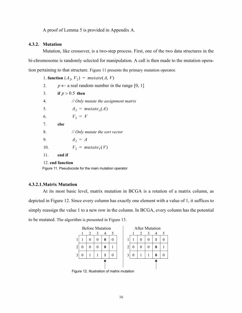
4.3.2.1.Matrix MutationAt its most basic level, matrix mutation in BCGA is a rotation of a matrix column, as

depicted in Figure 12. Since every column has exactly one element with a value of 1, it suffices to

simply reassign the value 1 to a new row in the column. In BCGA, every column has the potential

to be mutated. The algorithm is presented in Figure 13.

1. function

2.

3. if then

4. // Only mutate the assignment matrix

5.

6.

7. else

8. // Only mutate the sort vector

9.

10.

11. end if

12. end function

A2 V2,( ) mutate A V,( )=p a real random number in the range [0, 1] ←

p 0.5>

A2 mutateA A( )=V2 V=

A2 A=V2 mutateV V( )=

Figure 11. Pseudocode for the main mutation operator

1 2 3 4 51

2

3

0 0

0 0 0 1

0 1 1 1

1 0 0

0

0

Before Mutation After Mutation1 2 3 4 5

1

2

3

0 0

0 0 0 1

0 1 1 0

1 0 1

0

0

Figure 12. Illustration of matrix mutation

16

Lemma 6: The mutation of a valid assignment matrix results in a valid assignment matrix.

Proof: Since only the location of a 1 in a particular column has changed as a result of the muta-

tion operator, those properties of the column that are relevant to Rule A1 and Rule A2 are pre-

served, and the resulting matrix is valid.

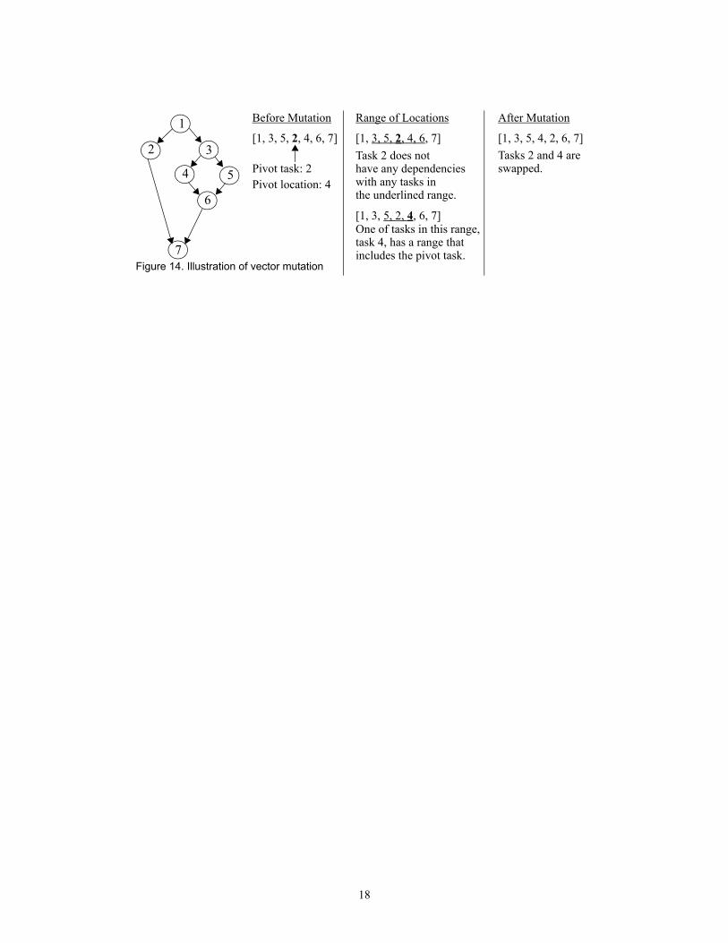
4.3.2.2.Vector MutationMutating the topological-sort vector is a two-phase operation that results in two tasks

swapping locations within the vector. First, a pivot task, , is randomly selected, and a range of

locations for which that task may be placed so that it is not placed before a predecessor or after a

successor in the transitive closure of the task graph is determined by the function

(Figure 16). Each task that lies the range of potential locations is then

similarly examined for the locations where it may be placed. Among those tasks whose range of

potential locations includes the pivot location, one is randomly selected, and that task is swapped

in the vector with the pivot task. The code is formally presented in Figure 15. An example of the

crossover operator is presented in Figure 14.

1. function

2. // Scan through each column of the matrix, and, with a probability of P,

3. // mutate the column. P is set to 0.2 in BCGA.

4. for begin

5.

6. if then

7.

8.

8.

10. end if

11. end for

12. end function

A mutateA B( )=

j 1…N=p a real random number in the range [0, 1]←

p P<

r a random integer in the range [1,P]←

aj the zero column←

arj 1←

Figure 13. Pseudocode for mutateA()

vj

potentialLocations V j,( )

17

[1, 3, 5, 2, 4, 6, 7]

Before Mutation

Pivot task: 2Pivot location: 4

1

2 3

4 5

6

7

[1, 3, 5, 2, 4, 6, 7]

Range of Locations

[1, 3, 5, 4, 2, 6, 7]

After Mutation

Task 2 does nothave any dependencieswith any tasks inthe underlined range.

[1, 3, 5, 2, 4, 6, 7]One of tasks in this range,task 4, has a range thatincludes the pivot task.

Tasks 2 and 4 areswapped.

Figure 14. Illustration of vector mutation

18

1. function

2.

3. // Scan through each element of the vector and, with a probability P,

4. // mutate that location of the vector. This implies that the task at that

5. // location is the pivot task for the mutation. In BCGA, P is set to 0.2.

6. for begin

7.

8. if then

9.

10. // Determine the contiguous locations where task

11. // vj can be placed.

12.

13. // For each location in the range r, determine which

14. // location possess tasks that can swap with task vj

15. for each begin

16.

17. if then

18. end for

19. // Swap task vj with a random task from the set swappable

20.

21.

22. end if

23. end for

24. end function

V mutateV W( )=V W←

j 1…N=p a real random number in the range [0, 1]←

p P<

swappable ∅{ }=

r potentialLocations V j,( )=

k r∈

q potentialLocations V k,( )=j q∈ swappable swappable k{ }∪←

i a random number from the set swappable←

swap vj vi,( )

Figure 15. Pseudocode for mutateV()

19

Lemma 7: The mutation of a valid topological sort vector results in a valid topological sort vec-

tor.

Proof: Suppose two tasks and , for , are swapped in a vector . Then, by the

algorithm , it is guaranteed that no task in the range is a prede-

cessor of or a successor of in the transitive closure of , and, furthermore, .

Therefore, no violations of the ordering of tasks in the vector result from the mutation, and the

vector is properly constructed.

4.3.3. SelectionUnlike the crossover and mutation operators, the selection operation cannot be performed

exclusively within the coordinate system since that space does not store the timing infor-

mation of tasks. Therefore, it is necessary to convert each solution representation into its corre-

sponding schedule, via , to determine its makespan, which is used as the measure of

fitness. BCGA uses roulette-wheel selection [1] as the basis for selection.

1. function

2. // Scan the locations to the right of the pivot location

3. for begin

4. if then

5. else break;

6. end for

7. // Scan the locations to the left of the pivot location

8. for downto begin

9. if then

10. else break;

11. end for

12. end function

locations potentialLocations V j,( )=

i j 1+( ) to N=vj succ

G+ vi( )∉ locations locations i{ }∪←

i j 1–( )= 1vj pred

G+ vi( )∉ locations locations i{ }∪←

Figure 16. Pseudocode for potentialLocations()

vj vk 1 j k N≤<≤ V

potentialLocations vi j i k< <

vj vk G vj succG+ vi( )∉

A V,( )

CS A V,( )

20

4.3.4. Initializing the PopulationGenerating random solutions for the initial population in BCGA requires the generation of

both randomized task-to-processor assignment matrices and randomized topological-sort vectors.

A well-randomized population consisting of valid representations is easily constructed if, for each

solution, exactly one 1 is randomly assigned to each column of the assignment matrix and if a

topological sorting algorithm, capable of randomly selecting tasks among a set of ready tasks, is

used for preparing the sort vector.

4.4. The Meta-OptimizationAs stated previously, BCGA is a genetic algorithm capable of generating solutions for the

multiprocessor scheduling problem. In order to increase its efficiency, the techniques of clustering

and merging are incorporated into the search process. Illustrated in Figure 2 is the optimization

process, called the meta-optimization, that uses BCGA.

The following details the precise implementation of each phase and the relationships

among them.

4.4.1. ClusteringThough it is not a necessary component to produce valid solutions, the effect that cluster-

ing has upon BCGA’s performance is substantial. The clustering phase produces sub-optimal

schedules for the task scheduling problem, but it ignores the required processor constraint. The

resulting clusters are used by the merging phase as a partial basis for the solution space. Because

the number of clusters can, at most, equal the number of tasks in the graph, clustering can poten-

tially reduce the size of the solution space and, consequently, the complexity of the search.

Dominant Sequence Clustering (DSC) [12] was the clustering algorithm of choice in

BCGA’s framework because it is able to generate high-quality clustering configurations in an

experimentally-negligible amount of time. Experiments comparing the performance of BCGA

over various clustering schemes including DSC (without a processor constraint), a genetic algo-

rithm, and no clustering not only verified the value of clustering as a critical component in optimi-

zation, but it also indicated that significant time tolerances dedicated to the clustering phase

21

(resulting in less time for the remaining phases) decreased BCGA’s performance. DSC provided

the best balance between time and performance for BCGA’s optimization framework.

The clustering configuration produced by the clustering phase is stored in a task-to-cluster

assignment matrix, termed the key in BCGA. It is used by the merging phase in the conversion of

clusters to individual tasks during the scheduling portion of the selection operator.

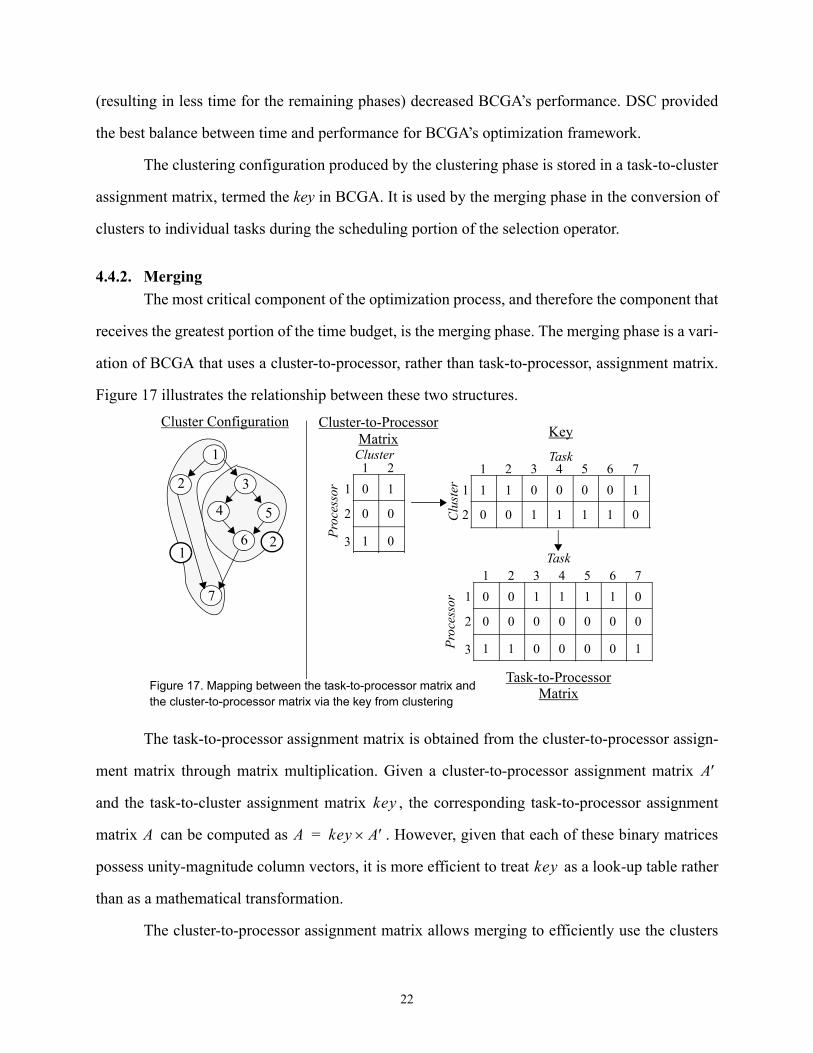
4.4.2. MergingThe most critical component of the optimization process, and therefore the component that

receives the greatest portion of the time budget, is the merging phase. The merging phase is a vari-

ation of BCGA that uses a cluster-to-processor, rather than task-to-processor, assignment matrix.

Figure 17 illustrates the relationship between these two structures.

The task-to-processor assignment matrix is obtained from the cluster-to-processor assign-

ment matrix through matrix multiplication. Given a cluster-to-processor assignment matrix

and the task-to-cluster assignment matrix , the corresponding task-to-processor assignment

matrix can be computed as . However, given that each of these binary matrices

possess unity-magnitude column vectors, it is more efficient to treat as a look-up table rather

than as a mathematical transformation.

The cluster-to-processor assignment matrix allows merging to efficiently use the clusters

1

2 3

4

6

7

5

12

Cluster Configuration

1 2 3 4 5 6 71

2

3

0 1 1 0

0 0 0 0 0

1 1 0 0 1

0 1 1

0 0

0 0

Clu

ster

Task1 2 3 4 5 6 7

1

2

1 0 0 1

0 1 1 1 1

1 0 0

0 0

1 21

2

3

1

0

1 0

0

0

Proc

esso

r

KeyCluster

Cluster-to-ProcessorMatrix

Task-to-ProcessorMatrix

Task

Proc

esso

r

Figure 17. Mapping between the task-to-processor matrix and the cluster-to-processor matrix via the key from clustering

A′

key

A A key A′×=

key

22

generated by the clustering phase. Because the topological-sort vector does not recognize clusters,

the use of clusters in the assignment matrix will not interfere with the execution order of individ-

ual tasks.

The cluster-to-processor assignment matrix is structurally equivalent to a task-to-proces-

sor assignment matrix, and, therefore, it follows the same rules for construction. For this reason,

the cluster-to-processor, rather than task-to-processor, assignment matrix is used directly by the

crossover and mutation operators of the merging phase.

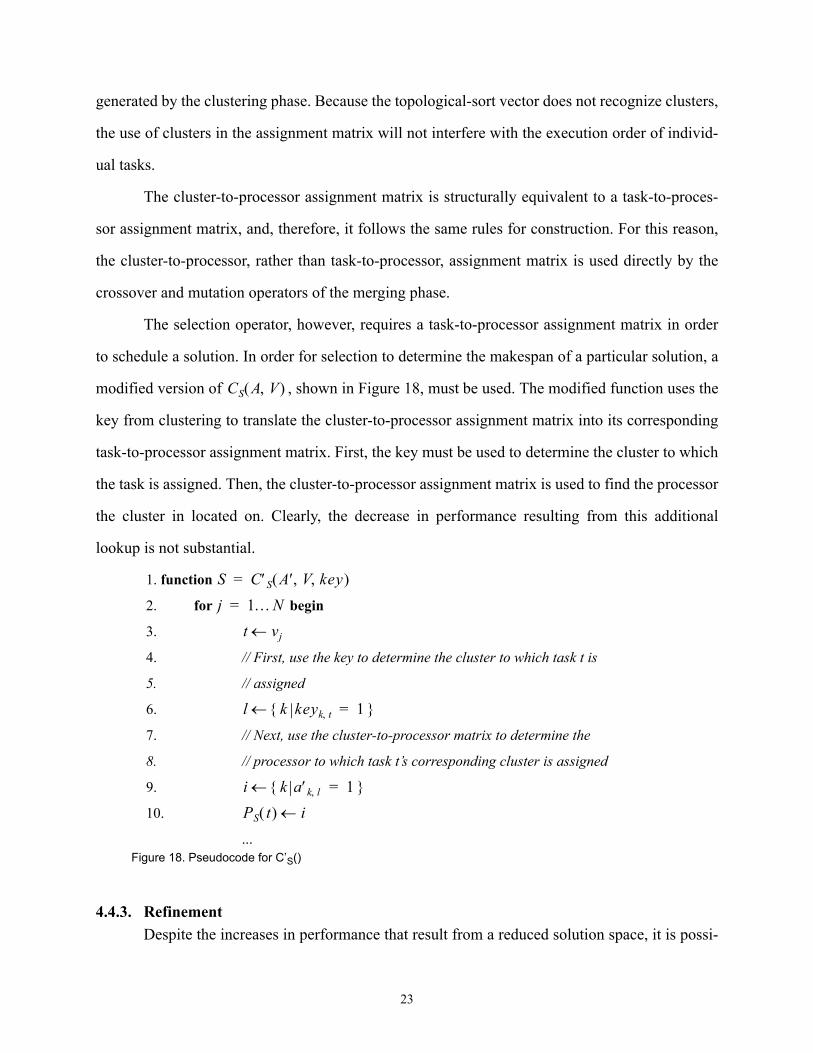
The selection operator, however, requires a task-to-processor assignment matrix in order

to schedule a solution. In order for selection to determine the makespan of a particular solution, a

modified version of , shown in Figure 18, must be used. The modified function uses the

key from clustering to translate the cluster-to-processor assignment matrix into its corresponding

task-to-processor assignment matrix. First, the key must be used to determine the cluster to which

the task is assigned. Then, the cluster-to-processor assignment matrix is used to find the processor

the cluster in located on. Clearly, the decrease in performance resulting from this additional

lookup is not substantial.

4.4.3. RefinementDespite the increases in performance that result from a reduced solution space, it is possi-

CS A V,( )

1. function

2. for begin

3.

4. // First, use the key to determine the cluster to which task t is

5. // assigned

6.

7. // Next, use the cluster-to-processor matrix to determine the

8. // processor to which task t’s corresponding cluster is assigned

9.

10.

...

S C′S A′ V key, ,( )=j 1…N=

t vj←

l k{ keyk t,← 1}=

i k a′k l,{← 1 }=PS t( ) i←

Figure 18. Pseudocode for C’S()

23

ble that the new space, determined by the clustering arrangement, does not possess an optimal

configuration for the original problem. Increasing time tolerances, therefore, do not guarantee the

increased likelihood of the merging phase obtaining a global minimum among the set of all possi-

ble schedules. In fact, a global minimum is only possible, under all clustering configurations, if

the optimization process eventually returns to searching the entire solution space. The final phase

of the meta-optimization, refinement, is included as a means for offering BCGA the chance of

achieving a global minimum or, at least, the possibility of finding a better sub-optimal solution.

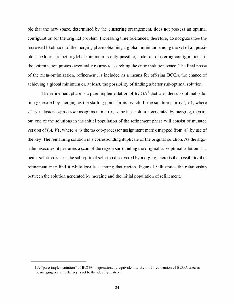
The refinement phase is a pure implementation of BCGA1 that uses the sub-optimal solu-

tion generated by merging as the starting point for its search. If the solution pair , where

is a cluster-to-processor assignment matrix, is the best solution generated by merging, then all

but one of the solutions in the initial population of the refinement phase will consist of mutated

version of , where is the task-to-processor assignment matrix mapped from by use of

the key. The remaining solution is a corresponding duplicate of the original solution. As the algo-

rithm executes, it performs a scan of the region surrounding the original sub-optimal solution. If a

better solution is near the sub-optimal solution discovered by merging, there is the possibility that

refinement may find it while locally scanning that region. Figure 19 illustrates the relationship

between the solution generated by merging and the initial population of refinement.

1.A “pure implementation” of BCGA is operationally equivalent to the modified version of BCGA used inthe merging phase if the key is set to the identity matrix.

A′ V,( )

A′

A V,( ) A A′

24

5. Experimental Results and AnalysisIn the experiments comparing BCGA1 and CGL, each genetic algorithm was required to

generate a 15-processor schedule for a given task graph in less than 9 hours of total execution

time. Such a relatively large time budget is reasonable in many embedded application domains

[6], where task graph scheduling is especially relevant. Because both algorithms rely upon the

transitive closure of the input graph, the time required to generate the transitive closure was not

accounted for in the compile-time budget.

5.1. The Test benchesIn order to fairly compare both algorithms, three distinct categories of graphs were used.

The first graph set, a series of application graphs presented by McCreary [7], provides a useful

comparison of the algorithms upon commonly-used graph structures. The second graph set is

composed of random graphs generated using an implementation of Sih’s algorithm [10]. The last

set of graphs are a series of random graphs presented by Kwok and Ahmad [4]. This last set of

graphs, referred to by the authors as random graphs with no known optimal solutions, provide a

1.It should be noted that BCGA in this section refers to the meta-optimization that includes BCGA.

In a merging phase, BCGA may find asolution that is a local maximum in thebroken-down solution space.

Other solutions inthe population.

The best solution from the merging phase(within the fully-sized solution space).

The local maximum in the smaller space ofmerging is, in the full space, surrounded bymore hills and valleys as presented in thiscontour map of the original local maximum inthe full space. (lighter areas indicate a higherfitnesses).

All but one solution ofinitial population aremutated versions of thebest solution from merging.The remaining one is theexact duplicate of thatsolution.

Figure 19. Illustration of the relationship between merging and refinement

25

comparison between the algorithms among three independently varying parameters: graph size,

communication-to-computation ratio (CCR), and graph width. Moreover, according to the

authors, the varied graph structures within this set should eliminate any bias a scheduling algo-

rithm may have towards a particular graph structure.

5.2. Portioning Time over BCGA’s Meta-FrameworkAs mentioned before, BCGA consists of three components over which the total compile-

time budget must be portioned. For this experiment, 0% of the time budget was allocated to clus-

tering, 70% to merging, and 30% to refinement. It must be noted that the deterministic algorithm

used for clustering, DSC, requires an insignificant amount of time to execute. Consequently, its

contribution to the time budget is approximated to 0%.

5.3. Results

5.3.1. McCreary’s Application GraphsThis set of application graphs1 provides a useful benchmark for comparing the perfor-

mance of BCGA and CGL within the context of real-world applications. Given the relatively

small size of these graphs, only one minute was allocated to the optimization. The results of the

experiments are summarized in Table 1.

Although BCGA outperformed CGL in the majority of the trials, the improvements are

1.A full description of each graph is available in [7].

Table 1: Comparison of BCGA and CGL on Application Graphs

Graph Nodes Edges CGL BCGA Relative %Improvement

K1 32 46 12 11 8.33%

NEQ 20 39 1596 1596 0.00%

IRR 41 69 600 580 3.33%

FFT1 28 32 152 124 18.42%

FFT2 28 32 270 240 11.11%

FFT4 28 32 260 255 1.92%

SUM1 15 14 53 39 26.42%

SUM2 15 14 36 37 -2.78%

26

irregularly distributed. These differences may be attributed to the performance of CGL. For

instance, DSC, the clustering algorithm used at the front-end of BCGA and the only non-random

component of the optimization, generates equal parallel times for graphs SUM1 and SUM2 [7].

Although BCGA dramatically outperforms CGL on SUM1, it slightly underperforms CGL on

SUM2. It is possible that the greedy scheduling heuristics in CGL optimize well for certain graph

structures, giving CGL an advantage for certain types of graphs and, possibly, hindering it on oth-

ers. With the exception of its clustering front-end, BCGA possess no knowledge of the scheduling

problem and, rather, performs a completely random search of the solution space.

5.3.2. Random Graphs Generated using Sih’s AlgorithmThe second set of benchmarks are random graphs generated using an implementation of

Sih’s algorithm. The graphs are designed to possess converging and diverging structures that

resemble, but are not modeled after, the patterns in existing application graphs. Table 2 summa-

rizes the results of these experiments.

Among this set of random graphs, BCGA outperformed CGL in 80% of the trials and,

among these, showed a significant improvement (more than 5%) in 25% of the tests.

5.3.3. Random Graph Provided by Kwok and AhmadThis set of graphs, categorized by Kwok et al. as random graphs with no known optimal

solutions, serve as the basis for the most comprehensive and informative set of tests. The bench-

marks, varying independently in size, CCR, and graph width, allow BCGA and CGL to be fairly

assessed upon a test bench that does not favor any particular scheduling strategy. The results are

Table 2: Comparison of BCGA and CGL on Graphs Generated by Sih’s Algorithm

Nodes Edges CGL BCGA Relative %Improvement Nodes Edges CGL BCGA Relative %

Improvement

154 175 82 77 6.10% 376 450 2164 2159 0.23%

168 189 124 114 8.06% 411 451 2268 2260 0.35%

252 350 156 149 4.49% 424 501 2216 2130 3.88%

326 330 1908 1908 0.00% 441 538 240 235 2.08%

341 369 185 189 -2.16% 456 520 2601 2556 1.73%

27

presented in Table 3.

In more than 80% of the trials, BCGA showed an improvement over CGL and, among

these, 65% were substantial improvements of at least 5%. However, as either the graph width or

CCR increased, the relative performance of the algorithms converged. It is conceivable that as

graph width, and consequently the amount of parallelism, increases, the effects of BCGA’s clus-

tering phase become less substantial.

It is similarly expected that as CCR increases the contribution of clustering will increase,

improving the performance of BCGA relative to CGL. However, this is not the case. It is possible

Table 3: Comparison of BCGA and CGL on random graphs with no known optimal solutions

Nodes Edges CCR CGL BCGA Relative% Imp. Nodes Edges CCR CGL BCGA Relative

% Imp.

Group 1: Average width is = Group 3: Average width is = 3

100 681 0.1 610 518 15.08% 100 556 0.1 825 768 6.91%

670 1 969 864 10.84% 582 1 1129 1027 9.03%

706 10 3521 3764 -6.90% 632 10 3397 3149 7.30%

200 1964 0.1 1352 1113 17.68% 200 1655 0.1 1519 1327 12.64%

2102 1 1964 1625 17.26% 1976 1 1845 1652 10.46%

2240 10 7494 7524 -0.40% 1726 10 8970 7611 15.15%

300 5381 0.1 1752 1411 19.46% 300 2752 0.1 2063 1804 12.56%

5381 1 2094 2159 -3.10% 3814 1 2785 2672 4.06%

5086 10 7564 7006 7.38% 3422 10 12331 11758 4.65%

Group 4: Average width is = 4 Group 5: Average width is = 5

100 507 0.1 830 782 5.78% 100 478 0.1 986 958 2.84%

394 1 1193 1162 2.60% 406 1 1215 1163 4.28%

569 10 4002 3724 6.95% 426 10 4410 4340 1.59%

200 1483 0.1 1476 1187 19.58% 200 1757 0.1 1520 1494 1.71%

1664 1 2020 1841 8.86% 1503 1 2293 2074 9.55%

1771 10 8215 7860 4.32% 1764 10 6966 9140 -31.21%

300 3697 0.1 2071 2064 0.34% 300 3185 0.1 2077 2084 -0.34%

3167 1 3083 3052 1.01% 2583 1 3214 3022 5.97%

2673 10 12618 15535 -23.12% 2857 10 13141 15450 -17.57%

node count node count

node count node count

28

that the improved performance of CGL relative to BCGA as CCR increases is due to the heuris-

tics in CGL, which may optimize well for high-CCR graphs.

6. SummaryThe well-studied field of multiprocessor scheduling has generated a number of genetic

algorithms dedicated to makespan minimization. However, all of these approaches share the com-

mon thread of a monolithic design that attempts to scan the entire solution space without consid-

eration to techniques that can reduce the complexity of this search. Even the substantial

improvements introduced in the CGL algorithm by Correa et al., a fairly expressive solution rep-

resentation and the incorporation of smart heuristics, resulted in increased complexity.

The improvements introduced by BCGA came not at the price of complexity, but directly

from simplification. The use of a bi-chromosomal representation in BCGA maintains the expres-

siveness of the string representation in CGL while reducing the of information contained within,

and, consequently, the restrictions placed upon, each independent structure. As a result, the com-

plexity of the crossover and mutation operators decreases, and the genetic algorithm is able to

more meaningfully explore the solution space.

Finally, the incorporation of clustering and merging into the meta-optimization of BCGA

serves to enhance its performance by dramatically reducing the size of the solution space. These

reductions significantly reduce the effort required by the crossover and mutation algorithms and

increase the efficiency of the search. BCGA’s bi-chromosomal representation facilitates the use of

this optimization hierarchy as it allows for clustering configurations to be used in the assignment

of tasks to processors without interference to task-execution order. Previous chromosomal repre-

sentations, such as the string representation which combines both task assignment and execution

order, cannot easily adopt clustering without incurring even greater algorithmic complexity.

7. Future WorkAn advantage to the multiphase layout of BCGA is the ability to manipulate certain

aspects of its design without the need to consider other independent phases. In particular is the use

29

of the DSC algorithm for the clustering portion of BCGA. Given the multitude of fast clustering

algorithms that exist for task scheduling, it may be advantageous to execute several, rather than

just one, clustering algorithm and then use the clustering configuration with the lowest makespan

as the key for the merging phase.

As stated previously, the total compile-time budget must be portioned over the three

phases in BCGA’s meta-optimization. In the experiments, the partition of 70% to merging and

30% to refinement was determined experimentally, but it was not examined in significant detail.

A closer examination of how time portioning affects the BCGA’s performance may be used to

improve the quality of the optimization.

Finally, it was shown by Correa et al. that significant improvements in multiprocessor

scheduling using genetic algorithms can be made by incorporating list heuristics into the genetic

operators. Experimentally, BCGA consistently, but not overwhelmingly, outperformed CGL. It

may be possible to further increase the effectiveness of BCGA by including heuristics, similar to

those used by CGL, into its operators.

30

Appendix A

Proof of Lemma 1: Given a schedule of task graph , the mapping via and

produces a valid pair and .

It must first be proven that the partial mapping via produces a valid matrix .

Rule A1 is satisfied since only assigns elements of the matrix with the values . Rule A2

is satisfied since every task in is assigned to, at most, one processor in :

Therefore, is valid.

Next, it is necessary to prove that the partial mapping via results in a valid vector

.

The proof that Rule V1 is satisfied by contraposition. Suppose contains the same task twice,

meaning that there exists a for which . For a single task to be located twice in , it

must have been selected twice from the set of remaining tasks. However, it must then follow that

, which is obviously not true.

On the other hand, suppose that does not contain a task from the graph, implying the task was

never selected for placement into by . Such an outcome would require that either or

that for every iteration of the algorithm. The former requirement is defeated

by the fact that, at the start of the algorithm, . The second requirement can only be satis-

fied if there is always a task in the set that contains an earlier start time than . However, for each of

the tasks in , a unique task must be selected on each of the iterations of . Since no task can

be selected twice, must eventually be placed in .

The proof that Rule V2 is also satisfied by contraposition. Suppose that the successor of a particu-

lar task is designated to execute before the task itself; that is, for some , .

For task to be selected before , the condition must be true. However, any

schedule that assigns a task to execute before its predecessor is an invalid schedule and, thus, Rule V2 is

satisfied.

Therefore, both and are valid.

Proof of Lemma 2: Given a valid solution pair , the mapping via will pro-

duce an executable schedule for the corresponding task graph .

If a schedule is executable, then it is implied that every task in the associated task graph fires once,

and that no processor executes more than once task simultaneously. Therefore, the conditions for an exe-

cutable schedule are:

S G S A V,( )→ CA S( )

CV S( ) A V

S A→ CA S( ) ACA S( ) A 0 1,{ }

G SPS tj( ) i k≠=( ) 1(⇒ aij aik 0 ) aj⇒=≠ 1= =

AS V→ CV S( )

VV

j k≠ vj vk t= = VTleft

t Tleft t{ }–∈

VV CV S( ) t Tleft∉

t mint Tleft∈ t startS t( ){ }∉

t Tleft(∈ T )=Tleft t

N G N CV S( )

t V

1 k j N≤<≤ vk succG+ vj( )∈

vk vj startS vk( ) startS vj( )≤

S

A V

A V,( ) A V,( ) S→ CS A V,( )

S G

31

• every task is scheduled exactly once

• a successor task is scheduled after all of its predecessors have been scheduled

• tasks on the same processor do not execute simultaneously

The first condition of executability can be proven by contraposition. Assume a schedule pro-

duced by has either scheduled a task more than once or not at all. Both of these conditions can

only be satisfied if either appears more than once or not at all in the topological-sort vector . A vector

with such a construction would violate Rule V1 and, therefore, would not be valid.

The second condition of executability is also proven by contraposition. Assume a schedule pro-

duced by has scheduled a task before its predecessor . This condition can only be satisfied if

either appears before in the vector or if the starting time of is scheduled before completes its

firing. The former condition cannot be true since a vector with such a construction would violate Rule V2.

The latter condition must be invalidated by induction.

By lines 13 and 15 of , it is impossible for a task to possess a starting time earlier than

any of its immediate predecessors’ finishing times. Likewise, the starting times of ’s the immediate pre-

decessors cannot occur before any of their predecessors’ finishing times, and so on. Therefore, by the tran-

sitive property of inequality, cannot have a starting time that occurs before the finishing times of any of

its predecessors in the transitive closure. The base condition for this induction is the starting times of the

root tasks of the graph, which possess no predecessors.

Finally, the last condition of executability requires that no tasks assigned to the same processor

execute simultaneously. By lines 14 and 15 of the pseudo-code for , it is impossible for the start-

ing time of a task to be scheduled before the finishing times of the previously-scheduled tasks on the same

processor. The tasks must be executed serially, and the last condition is satisfied.

Therefore, is executable.

Proof of Lemma 3: Given the set of mappings , the mapping is

unique in for all .

The proof of Lemma 3 simply requires that if , then . This rela-

tion implies that the conditions , , and

must be satisfied for all .

The first condition of equality is easily proven by substitution:

for all by

for all by

for all .

The proof for the second and third conditions is by induction. We want to show that if the prede-

SCS A V,( ) t

t V

SCS A V,( ) u t

u t V u t

CS A V,( ) uu

u

CS A V,( )

S

P A V,( ) S A V,( )→{ }= A V,( ) S→

S A V,( ) P∈

S′ Cs CA S( ) CV S( ),( )= S′ S=PS ′ t( ) PS t( )= startS ′ t( ) startS t( )=

finishS ′ t( ) finishS t( )= t

ait 1=( ) PS t( )⇔ 1= t CA S( )

PS ′ t( ) 1= a( it⇔ 1 )= t CS A V,( )

PS ′ t( )∴ PS t( )= t

32

cessors of those tasks on the same processor scheduled before a task are equivalently scheduled in and

, then must also be equivalently scheduled in both schedules.

Assume that for all the predecessors of task , , that the starting and finishing times

for each of these tasks are the same in both schedules ( and

). Furthermore, assume that every task that is assigned to the same proces-

sor as and scheduled before , that and . The start-

ing time of may be computed in the schedule by the following algorithm

However, the same algorithm is used for scheduling in if is replaced by in the code.

Assuming the base conditions are true, has the same starting time and finishing time in and .

For completeness of the induction argument, it is now only necessary to prove that the base condi-

tion holds. It will be shown that the root tasks of that are scheduled first in possess the same start and

finishing times in .

Let

By , for each task in as no task in that set possesses a predeces-

sor.

By , each task in will be placed in before any successors of another task in

if such successor tasks are assigned to the same processor. Consequently, will compute

.

It now follows that and

for all . The base condition is satisfied.

Therefore, .

Proof of Lemma 5: Given two proper valid vectors and , will generate a proper

child vector .

The proof that satisfies Rule V1 is by contraposition. Suppose that an arbitrary task appears

twice in . That is, for some , there exists a . This condition implies that task was selected

twice by from the set of tasks. However, for a task to be selected twice,

either or . Obviously, neither of these requirements can be true and, there-

t SS′ t

t a predG t( )∈

startS ′ a( ) startS a( )=finishS ′ a( ) finishS a( )= b

t startS ′ b( ) startS b( )= finishS ′ b( ) finishS b( )=t S

Tpred predG t( )←

Tproc a{ PS a( )← i}=startpred maxa Tpred∈ finishS a( ) ipcG a t,( )+{ }←

startproc maxa Tproc∈ finishS a( ){ }←

startS t( ) max startpred startproc,{ }←

finishS t( ) startS t( ) delayG t( )+←

t S′ S S′t S S′

G SS′

Troot t{ t roots G( ) and startS t( )∈ 0}= =CS A V,( ) startpred 0= Troot

CV S( ) Troot V Troot

CS A V,( )

startproc 0=startS ′ t( ) max startpred startproc,{ } 0 startS t( )= = =

finishS ′ t( ) delay t( ) finishS t( )= = t Troot∈

S CS CA S( ) CV S( ),( )=

W X crossoverV W X,( )

V

V tV j k≠ vj vk= tcrossoverV W X,( ) ready

t ready t{ }–∈ t succ t( )∈

33

fore, each element of the vector is unique.

On the other hand, assume that a task is not selected by the algorithm for placement into . For

a task not to be selected by , it is necessary that .

However, because no task can be selected twice, and because the algorithm will select one of a finite num-

ber of tasks on each of its iterations, every task must eventually be selected and scheduled.

Therefore, Rule V1 is satisfied.

The proof that satisfies Rule V2 is also by contraposition. Suppose that two tasks in are

placed in such a manner as to invalidate the topological sort. That is, for some ,

. For task to be selected before , must appear before in either of the two par-

ent vectors if is to produce first. However, either parent that satisfies this

property is not valid.

Therefore, Rule V2 is satisfied, and is valid.

References1. T. Back, U. Hammel, and H-P Schwefel. “Evolutionary Computation: Comments on the History and Current State,” IEEE

Transactions on Evolutionary Computation, vol. 1, no. 1, pp. 3-17, April 1997.

2. R. C. Correa, A. Ferreira, and P. Rebreyend. "Scheduling Multiprocessor Tasks with Genetic Algorithm," IEEE Transactions

on Parallel and Distributed Systems, vol. 10, no. 8, pp. 825-837, August 1999.

3. E.S.H. Hou, N. Ansari, Hong Ren. "A Genetic Algorithm for Multiprocessor Scheduling," IEEE Transactions on Parallel and

Distributed Systems, vol. 5, no. 2, pp. 113-120, February 1994.

4. Y.-K. Kwok, I. Ahmad. "Benchmarking and Comparison of the Task Graph Scheduling Algorithms," Proceedings of the 12th

International Parallel Processing Symposium, April 1998, pp. 531-537.

5. Y. Kwok and I. Ahmad. “Dynamic Critical Path Scheduling: An Effective Technique for Allocating Task Graphs to Multipro-

cessors,” IEEE Transactions on Parallel and Distributed Systems, vol. 7, no. 5, pp. 506-521, May 1996.

6. P. Marwedel and G. Goossens, editors. Code Generation for Embedded Processors. Kluwer Academic Publishers, 1995.

7. C.L. McCreary, A.A. Khan, J.J. Thompson, M.E. McArdle. "A Comparison of Heuristics for Scheduling DAGS on Multipro-

cessors," Proceedings of the 8th International Parallel Processing Symposium, April 1994, pp. 446-451.

8. V. Sarkar. Partitioning and Scheduling Parallel Programs for Multiprocessors. MIT Press, 1989.

9. G. C. Sih and E. A. Lee. “A Compile-Time Scheduling Heuristic for Interconnection-Constrained Heterogeneous Processor

Architectures,” IEEE Transactions on Parallel and Distributed Systems, vol. 4, no. 2, pp. 75-87, February 1993.

10. G. C. Sih. Multiprocessor Scheduling to Account for Interprocessor Communication. Ph.D. thesis, Department of Electrical

Engineering and Computer Sciences, University of California at Berkeley, April 1991.

11. Pai-Chou Wang, W. Korfhage. "Process Scheduling with Genetic Algorithms," Proceedings of the 7th IEEE Symposium on

Parrallel and Distributed Processing, October 1995, pp. 638-641

Vt V

crossoverV W X,( ) t minj 1 N,[ ]∈ j pj ready∈{ }∉

V V1 j k N≤<≤

vj succG+ vk( )∈ vk vj vk vj

minj 1 N,[ ]∈ j pj ready∈{ } vk

V

34

12. T. Yang and A. Gerasoulis. “DSC: Scheduling Parallel Tasks on an Unbounded Number of Processors,” IEEE Transactions

on Parallel and Distributed Systems, vol. 5, no. 9, pp. 951-967, September 1994.

35