WP/13/5

A Modern History of Fiscal Prudence and Profligacy

Paolo Mauro, Rafael Romeu, Ariel Binder, Asad Zaman

© 2013 International Monetary Fund WP/13/5

IMF Working Paper

Fiscal Affairs Department

A Modern History of Fiscal Prudence and Profligacy

Prepared by Paolo Mauro, Rafael Romeu, Ariel Binder, Asad Zaman1

January 2013

Abstract

We draw on a newly collected historical dataset of fiscal variables for a large panel of countries—to our knowledge, the most comprehensive database currently available—to gauge the degree of fiscal prudence or profligacy for each country over the past several decades. Specifically, our dataset consists of fiscal revenues, primary expenditures, the interest bill (and thus both the primary and the overall fiscal deficit), the government debt, and gross domestic product, for 55 countries for up to two hundred years. For the first time, a large cross country historical data set covers both fiscal stocks and flows. Using Bohn’s (1998) approach and other tests for fiscal sustainability, we document how the degree of prudence or profligacy varies significantly over time within individual countries. We find that such variation is driven in part by unexpected changes in potential economic growth and sovereign borrowing costs.

JEL Classification Numbers: H62, H63

Keywords: Fiscal policy, public debt, budget deficits, economic growth, debt sustainability

Authors’ E-Mail Addresses: pmauro@imf.org, rromeu@imf.org, abinder@imf.org, azaman@imf.org

1 We thank Olivier Blanchard, Carlo Cottarelli, Mark De Broeck, Jonathan Ostry, and participants in seminars in the IMF’s Fiscal Affairs and Research Departments for helpful suggestions, as well as Verena Grass and Juliana Peña for help with some of the archival and data research.

This Working Paper should not be reported as representing the views of the IMF. The views expressed in this Working Paper are those of the author(s) and do not necessarily represent those of the IMF or IMF policy. Working Papers describe research in progress by the author(s) and are published to elicit comments and to further debate.

2

Contents Page

I. Introduction ............................................................................................................................4 

II. Data Sources and Basic Statistics..........................................................................................6 A. Data Sources for Fiscal and Other Macroeconomic Variables .................................6 B. Summary Statistics for Main Fiscal Aggregates .......................................................8 C. Data Sources for Other Variables ............................................................................10 

III. Measuring Fiscal Prudence/Profligacy ..............................................................................12 A. Bohn’s Fiscal Reaction Function and Policymakers’ Criterion ..............................12 B. Methods to Gauge Variation in Prudence/Profligacy Over Time ...........................14 C. The Drivers of Changes in Fiscal Prudence/Profligacy ..........................................15 

IV. Estimates of Fiscal Prudence/Profligacy ...........................................................................16 A. Bohn (1998) Tests for Whole Sample Periods and Long Sub-Samples, Individual Countries ................................................................................................16 B. Structural Breaks .....................................................................................................17 C. Search for Influential Observations.........................................................................18 D. Rolling (Fixed-Length) Windows and Increasing Sample Periods ........................19 E. Summarizing the Historical Assessment of Prudence and Profligacy ....................21 

V. The Drivers of Changes in Fiscal Prudence/Profligacy ......................................................22 

VI. Conclusions........................................................................................................................24  Tables 1.  Country Coverage of Main Variables in this Study ...........................................................26 2.  Summary Statistics for Full Sample (1800 – 2011) ...........................................................27 3.  Summary Statistics for Post-WWII (1950-2011) ..............................................................28 4.  Summary Statistics for Advanced Economies ...................................................................29 5.  Decomposition of Variance of Debt Changes, Advanced Economies (1950-2011) .........30 6.  Decomposition of Variance of Debt Changes, Emerging Economies (1950-2011) ..........31 7.  Bohn (1998) Test for Fiscal Policy Sustainability .............................................................32 8.  Bohn Regression Results Iterated Over Twenty-Five Year Rolling Windows .................33 9.  Bohn (1998) Fiscal Reaction Function with Expanding Sample .......................................34 10. Structural Breaks in Bohn (1998) Sustainability Test, Post-War ......................................35 11. Structural Breaks in Bohn (1998) Sustainability Test, Full Sample ..................................36 12. Influential Years in Recursive Bohn (1998) Test ..............................................................37 13. Times of Strong Prudence and Profligacy .........................................................................38 14. Panel Results, Fiscal Response as a Function of Growth and Borrowing Costs ...............39  Figures 1.  Government Debt and Primary Fiscal Balance, 1850−2011, in percent of GDP ..............40 2.  Fiscal Variables (Top Chart) and Rolling Regression Results for Japan, 1875-2011 .......41 3.  Periods of Prudence and Profligacy, 1800-2011................................................................42 

3

4.  Periods of Prudence and Profligacy, 1850-2011................................................................43 5.  Periods of Prudence and Profligacy, 1850-2011................................................................44 6.  Periods of Prudence and Profligacy, 1880-2011................................................................45 7.  Periods of Prudence and Profligacy, 1880-2011................................................................46 8.  Periods of Prudence and Profligacy, 1900-2011................................................................47 9.  Periods of Prudence and Profligacy, 1900-2011................................................................48 10. Periods of Prudence and Profligacy, 1950-2011................................................................49 11. Periods of Prudence and Profligacy, 1960-2011................................................................50  References ................................................................................................................................51 

4

I. INTRODUCTION

The terms “fiscal prudence” and “fiscal profligacy” are often used, somewhat loosely, to denote whether fiscal policies tend to lead to a sustainable or unsustainable fiscal position. The latter would correspond, in more academic terms, to whether the government’s intertemporal budget constraint is met—that is, whether the expected present discounted value of all future fiscal surpluses matches the existing stock of public debt. Although a precise definition of prudence or profligacy has not been established, policymakers, investors, and voters need to take a view all the time, in real time, on whether a country’s fiscal policies are appropriate to support economic growth and achieve other social objectives without causing a fiscal crisis. The focus is on the fiscal stance within the control of the government—usually proxied by the primary fiscal balance (i.e., the fiscal balance net of interest payments). In practice, prudence and profligacy are medium-term concepts. Neither prudence nor profligacy is built up overnight: one or even a few years of expansionary fiscal policies do not necessarily cause a fiscal crisis, if a government’s initial position is sufficiently strong. Conversely, one cannot expect that, in real life, people will wait until infinity to check whether the intertemporal budget constraint is met. A few years of sustained deficits could well suggest that the intertemporal budget constraint is at risk. Thus, judgments regarding whether prudence or profligacy prevails are necessarily made over the course of a few years. Moreover, we believe (and show empirically below) that a country’s degree of prudence or profligacy is not constant forever; rather, it will change over time, as governments, citizens’ attitudes, and economic circumstances change. This paper draws on a newly collected historical dataset of fiscal variables for a large panel of countries—to our knowledge, the most comprehensive database currently available—to gauge the degree of fiscal prudence or profligacy for each country over the past several decades. Specifically, our dataset consists of fiscal revenues, primary expenditures, the interest bill (and thus both the primary and the overall fiscal deficit), the government debt, and gross domestic product, for 55 countries for up to two hundred years. For the first time, a large cross country historical data set covers both fiscal stocks and flows. Unfortunately, the economics profession has not yet developed a universally accepted indicator of fiscal sustainability. We rely heavily on the work of Bohn (1998, 2008), which we consider to be the “state of the art” in this area. Bohn’s sustainability criterion is based upon a time series regression of the primary fiscal surplus on the public debt and other controls.2 Thus far, empirical application of the Bohn test has been constrained by data limitations. Bohn’s own work analyzed long run historical time series data for the United 2 Other tests based on the univariate time-series behavior of the debt-to-GDP ratio have fallen by the wayside, because of the difficulties in detecting mean-reversion as the debt-to-GDP ratio is bounced around by various shocks (see Bohn, 1998, 2007, and citations therein). Again, the weaknesses of tests based upon a univariate analysis of the debt-to-GDP ratio point to the value added of our dataset which, in addition to the stock of debt, also reports data on flows.

5

States. A more recent study by Mendoza and Ostry (2008) analyzed panel data for 34 emerging markets and 22 advanced economies over the period 1990–2005, but the relatively short time period for which data were available required constraining the estimated fiscal policy response coefficient to be the same across the advanced economies and across the emerging markets. Our data collection effort makes it possible for the first time to run this test for individual countries, for a large number of countries. A possible drawback of Bohn’s test is that it estimates the policy response over a long time frame of many years. Because our purpose is to explore variation in the fiscal policy response function across countries but also over time within a given country, we relax Bohn’s assumption of a constant long term fiscal policy response. Specifically, for each country, we employ three variations of the standard Bohn regression, including structural break tests, recursive searches for particularly influential observations, and iterations of the standard regression over rolling subsamples. We also complement these exercises with a simpler “policymakers’ criterion” widely used among practitioners, which consists of comparing the actual primary surplus to the primary surplus that would be required to stabilize the debt-to-GDP ratio.3 By algorithmically combining these criteria, we believe we provide a reasonable gauge of the degree of fiscal prudence or profligacy for each country at various points in time. More generally, our paper follows a well established tradition in drawing lessons relevant to modern themes from long-run historical panel data sets (recent examples include Reinhart-Rogoff, 2009 and 2011 for public debt; and Schularick and Taylor, forthcoming, for credit aggregates). While we use the terms “prudence” and “profligacy” for presentational simplicity, we attribute to them specific, positive, technical meaning as described in the body of the paper, rather than necessarily normative meaning. In other words, “profligate” fiscal policy responses may sometimes be justified from a normative standpoint—for example, to avoid plunging the economy into a deep and prolonged recession. The analysis in this paper is primarily positive. Our main findings are the following:

For most advanced countries, particularly prior to the global economic and financial crisis that began in 2008, we find evidence that the response of the primary fiscal surplus to variation in government debt is consistent with meeting the intertemporal budget constraint, as well as stationarity of the debt.

Nevertheless, the evidence suggests that a given country’s fiscal policy response to changes in debt is by no means constant throughout its history (a working assumption that previous studies had made owing to data limitations). On the contrary, we document

3 The policymakers’ criterion checks whether fiscal policy is consistent with stability of the debt ratio, a special case of the stationarity that is assessed through the Bohn test.

6

significant variation in such response, not only across countries, but also over time within a given country. Periods of a few or more years are distinguishable as clearly “prudent” or “profligate,” often with all techniques giving consistent messages. Indeed, one of the paper’s contributions is to document how individual countries fare with respect to fiscal prudence and profligacy, using each of the methods outlined above. Individual country results are reported in detail in this working paper’s tables and charts, with further information reported in the country pages in the accompanying Chartbook.

For example, the results suggest widespread fiscal prudence in most advanced economies

during the mid-1990s until at least the mid-2000s; for the emerging economies, prudence becomes more widespread after the year 2000. Strong prudence is evident in the United States in the late 1990s (recalling contemporary discussion of a possible disappearance of the public debt); in Canada since the mid-1990s (beginning with an ambitious and successful fiscal adjustment plan); in several Euro area countries during the mid-1990s (coinciding with the Maastricht Euro entry process); in Ireland in the late 1980s and early 1990s (a well known fiscal adjustment episode); in Japan in the mid-1980s to early 1990s (as it sought to stabilize the debt); and in Turkey in the mid-1990s and at several points in the 2000s (as it improved its primary balance significantly). Conversely, notable episodes of fiscal stimulus are also evident, including the United States in 2009–11 and Spain in 2010. And Japan is found not to sufficiently improve its primary balance despite rising debts for several years starting in the late 1990s.

Finally, we show that a stronger response of the primary fiscal balance to changes in

government debt is significantly associated with changes in long-run real GDP growth rates and long-term sovereign borrowing costs (measured by secondary market interest rates on long-term government debt). Declines in “potential” (or long-run) economic growth may not be fully apparent in real time to contemporary policymakers, who therefore often fail to respond to such declines through sufficient improvements in the primary balance. Conversely, increases in the cost of sovereign borrowing prompt policymakers to tighten fiscal policy in response.

The remainder of the paper is organized as follows. Section II outlines the data collection process and reports the summary statistics. Section III presents our empirical approach and its underpinnings. Section IV reports the empirical results. Section V concludes.

II. DATA SOURCES AND BASIC STATISTICS

A. Data Sources for Fiscal and Other Macroeconomic Variables

The database covers an unbalanced panel of 55 countries (24 advanced economies—by present day definition from the IMF’s World Economic Outlook classification—and 31 non-advanced) over 1800–2011. The data consist of government revenue, non-interest government expenditure, and the interest bill (and thus also the overall fiscal balance and the primary balance), as well as gross public debt, all expressed as a share of GDP. Table 1 reports the list of countries and the corresponding period for which we have data for all the variables mentioned above.

7

This database covers not only public debt stocks, but crucially, the corresponding fiscal balance flows and their subcomponents. The availability of data on the primary balance to accompany the corresponding public debt observations makes it possible to apply well established tests or criteria that seek to gauge the degree of sustainability of a country’s fiscal policies and public debt position. About half of the observations for the fiscal variables in our dataset are drawn from various cross-country sources, including the IMF’s World Economic Outlook (WEO) and International Financial Statistics (IFS) and the OECD Analytical Database for the past 20–50 years (subject to availability)4; the Statistical Yearbooks of the League of Nations and the United Nations (as well as their Public Debt Supplements) for the period between World War I and the 1970s (we collected these data by hand from various yearly reports); and Flandreau and Zumer (2004) for the pre-World War I era; in addition, long-run historical series are drawn from Mitchell’s International Historical Statistics and the Montevideo-Oxford Latin American Database (MOXLAD). We hand-collected the other half of the data from country-specific sources, such as official government publications or economic histories that included public finance statistics. Examples of such data sources include Fregert and Gustafsson (2005) for Sweden over 1800–2004; Fernandez and Acha (1976) for Spain over 1850–1975; and Junguito and Rincon (2004) for Colombia over 1923–2003. The list of all sources, with complete bibliographical and coverage information, is provided in Appendix Table 1 (see electronic chartbook). In collecting nominal GDP data for the distant past, we relied heavily on Mitchell and MOXLAD. For most countries, GDP data do not exist before World War I (indeed, the concept was not used by contemporaries), and in these cases we used proxy variables such as Gross National Product or Net National Product from Mitchell’s International Historical Statistics. In a few cases we used UN statistical yearbooks to fill in gaps in coverage between 1940 and 1975. GDP data were drawn from the OECD database for a few member countries beginning as early as 1960. For some countries, such as the United States, the United Kingdom, Italy, the Netherlands, Japan, Canada, and India, we used government publications or other country-specific sources. Starting in the mid 1990s, GDP data for almost all countries are taken from the WEO. Many sources, both cross-country and country-specific, provided fiscal data already expressed in terms of GDP as well. Given the availability of multiple sources with significant overlaps for each country, we report in detail the “decision tree” (see Appendix Figure 1 in electronic chartbook) we used to splice together different sources to create continuous historical series. Within each country, we sought to preserve source continuity across time, to minimize jumps in the series that would have stemmed solely as a result of changes in sources. Whenever possible, we also sought to draw all variables (particularly the fiscal variables) for each given year from a single data source, to preserve consistency across concepts. The splicing process was straightforward for countries without much source overlap or source disagreement, and for

4 We used the most recent published editions as of October 2011.

8

countries for which we found a source offering long, nearly uninterrupted coverage for all concepts of interest. When these conditions did not hold, preserving source continuity across time sometimes became at odds with preserving source consistency across concepts. In such cases, because the primary balance usually had to be computed as the difference between the overall fiscal balance and interest payments, and because the response of the primary balance to changes in public debt is a key object of interest in this paper, we generally preferred source consistency across concepts over continuity across time. For instance, even though Mitchell provides fairly comprehensive data on revenue and expenditure, we often took revenue and expenditure data from UN statistical yearbooks where they were available, because these yearbooks also provide data on interest payments and debt. This said, we sought to use a given data source for continuous stretches of at least ten years, unless shorter stretches were the only way to fill a gap. Appendix Table 2 (see electronic chartbook) reports, by country, the data source used for each concept at each point in time. An important issue in the construction of long term public finance data series relates to the choice of government sector coverage. We sought to use data referring to the most comprehensive sector of government for which they were available. Accordingly, we report data at the general government level where these are available. In most cases, general government data are impossible to come by before 1960—not surprisingly, given that for most countries the share of spending by sub-national governments has risen significantly only since then. As a result, the sector reported switches (in most cases, simultaneously for all variables for a given country) from central government to general government in nearly all final spliced series, and this switch generally happens in the 1960s or 70s. For countries with large and active subnational governments, such as most advanced countries, this change in sector coverage resulted in significant breaks in the revenue and primary expenditure series; the breaks in the debt and fiscal balance series were smaller. Breaks in series are recorded in the database through dummy variables.

B. Summary Statistics for Main Fiscal Aggregates

Figure 1 reports the simple and GDP-weighted averages and the median of the public debt stock (top panel) and the primary balance (middle panel), in percent of GDP, from 1850 to the present. The shaded areas represent the range between the 15th and 85th percentiles. The number of countries in each year for which both debt and primary balance data are available is also reported (bottom panel). We observe sharp decreases (increases) in the average primary balances (debts) during the World Wars. The range of both variables widens substantially during times of war, e.g. the U.S. Civil War. The primary deficits reverse quickly once the war episodes end, whereas postwar debts decline more gradually and over longer periods. Focusing on the post-WWII era, debt declines continuously until the 1970s, through a combination of negative interest-growth differentials together with stable and slightly positive average primary balances. From the 1970s, debts generally increased and the primary balances improved somewhat further. Strong improvements in the primary balance occurred in the second half of the 1990s, largely reflecting Maastricht-related fiscal consolidations. Noticeable worsenings in the primary balance occurred in the late 1970s, early 1980s, early 1990s, and early 2000s. The global economic and financial crisis of the

9

late 2000s resulted in the most pronounced and pervasive peacetime worsening of the primary fiscal balance experienced during our long term historical investigation: the average and GDP-weighted average primary deficits in 2008−09 were larger than at any other point in history aside from the World Wars. By way of comparison, the Great Depression is hardly noticeable in the chart. Table 2 provides summary statistics for the full sample period (1800−2011, subject to data availability) for the major budgetary line items, including revenues, expenditures, the public debt interest bill, the overall fiscal balance, the primary balance, gross public debt, and the interest-growth differential.5 The dataset consists of about 5,700 observations for each of revenue, expenditure, overall fiscal balance, and debt. Interest expenditure data, however, are limited to approximately 4,800 observations (and consequently primary expenditure and primary balance as well). Both debt and primary balance data are available for about 4,500 country-years. The revenue and expenditure ratios to GDP averaged 19 percent of GDP and 21 percent of GDP, respectively, while the public sector interest bill averaged 2½ percent of GDP. The primary surplus over the sample averaged ½ percent of GDP, debt averaged 50 percent of GDP, and countries generally faced a negative interest-growth differential. While both advanced and non-advanced countries maintain fiscal balances of similar magnitude, non-advanced economies report both lower revenues and expenditures. Advanced economies also report larger debt ratios, primary balances, and interest-growth differentials compared with the non-advanced. Primary surpluses in the top percentile are in excess of 9½ percent of GDP, though these largely correspond to commodity producers or countries with large government assets.6 Those in the top five percent of the distribution are above 5½ percent of GDP, and include several advanced economies with a well diversified production structure and relatively small government assets. Table 3 reports the summary statistics for the post-World War II period, 1950-2011. Significant differences are again observed between advanced and non-advanced economies, notably: (i) size of the public sector nearly twice as large in the advanced economies compared with the non-advanced; (ii) slightly larger debt ratios in the advanced economies (based on the median across countries); (iii) larger primary balances in the advanced economies; and (iv) more negative interest rate-growth differentials in non-advanced economies. Table 4 compares the post-war period with the period up to 1950 but excluding wars, for the advanced economies. The table shows the tripling of public sector revenues and expenditures

5 The interest-growth differential is the difference between the implied nominal interest rate (current year interest payments divided by the average of current and past year debt stock) and this year’s nominal GDP growth rate.

6 Gross debt is used throughout, and the primary balance is defined as the fiscal balance plus gross interest payments. Thus we do not subtract interest revenues, which would be appropriate if we used the net public debt.

10

relative to the pre-1950 period. Despite worsening primary balances and primary expenditure increasing fourfold after 1950, debt declined, consistent with the negative interest rate-growth differential observed after World War II. The broader increase in primary expenditure could also be interpreted as consistent with government size increasing with economic development and over time (“Wagner’s law”). To make the case that our main object of interest, the primary fiscal balance, is a key driver of variation in the debt-to-GDP ratio, we recall identity (2.1), which decomposes the change

in the debt-to-GDP ratio (∆ ) into the contributions from the primary fiscal balance ( ts ), the

interest rate-growth differential , and the stock-flow residual ( tSFR ).

11t t

t tt

t t

r gd SF

gd s R

(2.1)

As the variance of a sum can be expressed as the sum of the variances plus twice the sum of the covariances, we decompose the variance of the changes in the debt ratio into the sum of the variances and pairwise covariances of the primary deficit, the contribution from the interest-growth component, and the stock-flow residual. Table 5 and Table 6 show the variance decomposition results for advanced and non-advanced economies with more than 30 observations for 1950-2011, and excluding changes corresponding to shifts in government sector coverage. For advanced economies, high stock-flow residual variances broadly correspond to countries with sizable asset accumulation (e.g. Norway, Sweden, Finland, and Japan), and to Greece, which experienced high inflation and defaults at various points in the 1950s and 1960s, and again debt restructuring in 2011. The average and median values for advanced economies suggest that fluctuations in the primary balance, interest rate-growth differentials, and stock-flow changes each explain roughly one-third of the variance of changes in the debt ratio. For non-advanced economies, more volatile debt changes are in most cases explained largely by the volatility in the stock-flow residual and interest-growth differential, consistent with greater prominence of defaults, episodes of high inflation, and more frequent exchange rate crises. Nevertheless, there is great heterogeneity among the non-advanced economies. The factors underlying variation in debt for macroeconomically stable non-advanced economies, such as Colombia and India, are similar to those for advanced economies, whereas debt changes in several other non-advanced economies are driven almost entirely by the stock-flow residual.

C. Data Sources for Other Variables

Wars

Years in which major wars led to extraordinary, temporarily high expenditures are excluded in Table 4 and the tests below. This is consistent with Barro’s (1979) “tax-smoothing” reasoning and with Bohn’s (1998) empirical analysis of United States data, which reported specifications excluding World War II and its immediate aftermath. In the multinational context, we identified a list of country-years involving participation in major wars (from various encyclopedias) and then excluded from the sample those country-years where war

11

participation led to an increase in the expenditure-to-GDP ratio by at least six percentage points in one year. We also excluded up to two years after the war period, to allow for expenditures linked to demilitarization and reconstruction. Based on this criterion, we excluded country-years involving the Danish-Swedish War of 1808-1809, the United States Civil War, the Greco-Turkish War, World War I, World War II and the Indo-Pakistani War of 1971.7 Defaults

Years of default are drawn from Reinhart and Rogoff (2010) and are excluded from most empirical exercises. 8 Many Latin American economies in our sample experienced defaults, as did several European economies prior to and during World War II. Output and expenditure gaps

We compute output and expenditure gaps as percent deviations of real output and expenditure series from their Hodrick-Prescott-filtered trends.9 For nearly all countries in the sample, real output series are computed from Maddison data for the early period, and the World Development Indicators (WDI) database for real GDP data for later years.10 For most countries, WDI real GDP data begin in the 1960s or 1970s. From 2009 through 2016, real GDP data and projections are drawn from the WEO.11 Real expenditure series result from the product of expenditure-to-nominal GDP and real GDP. For expenditure data gaps of three years or fewer, interpolated real expenditure values are used. For countries with blocks of at least 25 years of continuous expenditure data separated by a gap of at least 4 years, the HP-filter was applied to the separate sample periods. In cases where the expenditure data unnaturally changed as a result of a shift in coverage of the levels of government, all general government real expenditure figures were multiplied by the ratio of central government expenditure to general government expenditure in the year of the sector switch. Commodity price indices

To control for the effects of commodity price swings on the primary balance of commodity producing countries, we include two world commodity price indices as additional 7 Specifically, beyond the many country-years for which data were already missing during war episodes, we excluded the following country-years: United States (1917-1919), United Kingdom (1914-1919), Italy (1914-1919), Sweden (1918), Finland (1918-1919), South Africa (1914-1915); United States (1942-1947), United Kingdom (1940-1947), Belgium (1943), Italy (1940-1946), Sweden (1940-1945), Switzerland (1940-1945), Canada (1940-1945), Finland (1939-1945), Australia (1943-1946), South Africa (1940-1945); United States (1862-1866); Sweden (1810); Greece (1897-1898); and Pakistan (1971).

8 Default years available at http://www.reinhartandrogoff.com/data/browse-by-topic/topics/7/.

9 This approach follows Mendoza and Ostry (2008).

10 Maddison does not cover Iceland, so Penn World Table data are used for years preceding WDI data.

11 For the United States, Sweden, Greece, and Argentina, fiscal data extend back further than Maddison, and in these cases real GDP data from national sources is used prior to Maddison, WDI, or WEO.

12

regressors—one index includes petroleum prices and the other does not. The source is MOXLAD for 1900−1957 and the IMF Research Department thereafter. The list of countries dependent on commodity exports and those dependent on energy exports more specifically are drawn from the WEO (which in turn derived its country groupings from export composition data for 1962−2010). Real long term interest rates

An objective of this paper is to explore potential determinants of variation—across countries and over time—in the fiscal policy response to increasing debt. To that end, in section V, we test the hypothesis that a higher marginal cost of sovereign borrowing (interest rates on government bonds observed on secondary markets) is associated with greater responsiveness of primary fiscal surpluses to government debt. Our real long term interest data consist of 2,270 observations and are mainly drawn from Bordo and others (2001), Dincecco (2011), and the IMF’s International Financial Statistics (IFS). Generally, Bordo and Dincecco cover the time period 1860−1947, whereas the IFS cover 1948−2011. In order to fill the gaps in our series we use several other cross-country databases as well as national sources (OECD; WEO; Mauro and others, 2006; IMF databases). Altogether, we have data for 27 countries with the series going back to the 1880s for the majority of the advanced economies.

III. MEASURING FISCAL PRUDENCE/PROFLIGACY

We now outline how the degree of fiscal prudence or profligacy can be measured, both across countries and at different points in time, and how “fiscal reaction” regression analysis needs to be extended to explore how fundamental economic variables shape the degree of responsiveness of fiscal policy.

A. Bohn’s Fiscal Reaction Function and Policymakers’ Criterion

The literature on debt sustainability has identified a limited set of somewhat crude indicators of what may be labeled as fiscal prudence. In what follows, we rely heavily on an approach developed by Bohn (1998), which is based on estimating the following “fiscal reaction” regression on time series data for a given country:

,t t t ts d Z (3.1)

where ts and td are the primary surplus and the beginning-of-period public debt,

respectively, both in percent of GDP; tZ captures other determinants of the primary balance,

such as the business cycle or war expenditure shocks; t is an error term.

Bohn (1998) shows that if is estimated to be positive and significant, then fiscal policy is

consistent with the intertemporal budget constraint under uncertainty, and that the test is robust to changes in interest rates, debt structure, and growth rates. Moreover, he shows that

if 1r g

r then the debt ratio is stationary: in the event of a shock to the debt ratio, the

13

fiscal policy response would be sufficiently strong to bring the debt ratio gradually back to its initial level. In our empirical applications, we will use medium run averages of r and g, as detailed in the next sections. Despite its many strengths, Bohn’s (1998) approach also has limitations. First, configurations of the debt ratio and ρ may emerge in which the primary fiscal surplus implied by the estimated fiscal policy reaction function is too high to be politically feasible or realistic. In the empirical applications, this limitation becomes relevant, as we show below. Second, the test was conceived against the background of a generally rising debt ratio. However, many countries experienced declining debt ratios for several decades: we would argue that, in that context, failure to obtain a positive and significant Bohn coefficient (which would require a worsening primary deficit) would indeed indicate an inconsistency with the intertemporal budget constraint but should be labeled as over-accumulation of assets rather than lack of fiscal prudence.12 We note such instances below when they occur. Third, many years of data are necessary for a regression to be estimated, but policymakers and others often need to come to a judgment on whether fiscal policy is appropriate over a shorter horizon. Thus, policymakers and analysts in international financial institutions and the private sector often rely on comparisons between the actual primary surplus and the primary surplus that would be needed to stabilize the debt ratio—we label this the policymakers’ criterion.13 From the well known debt motion equation, the debt-stabilizing

primary surplus is 11t t

t

r ggt ts d

. Note the close correspondence between the

policymakers’ criterion and Bohn’s criterion for stationarity of the debt ratio, as a stable debt ratio is a special case of a stationary debt ratio.14 15

12 In practice, the case in which the primary surplus is increased in response to a decline in public debt does not need to result in accumulation of assets during the sample period. More simply, the primary surplus increase would further accelerate the decline in the debt to the point where, if such behavior persisted, the country would eventually accumulate so many assets that some would be left over at infinity.

13 This simple approach has been widely used for several decades. In reviewing approaches to assessing fiscal sustainability, Blanchard (1990) refers to a “primary gap” defined as the difference between the primary fiscal surplus and the product of the debt ratio times the difference between the interest rate and the growth rate.

14 The careful reader will note that the policymakers’ criterion contains g in the denominator and a lagged debt, whereas Bohn’s condition for stationarity (which we present as in the original article) contains r in the denominator. This difference simply reflects different notation conventions in writing the debt motion expression. Bohn’s (1998) debt motion expression, based on beginning of period debt, assumes that interest is paid on the difference between this year’s debt stock and this year’s primary surplus, whereas in (2.1) and thus the policymakers’ criterion we use the more standard assumption that interest is paid on last year’s debt stock.

15 A fourth limitation, which admittedly is not addressed by the policymakers’ criterion either, relates to the fact that the Bohn coefficient could signal lack of prudence in case the primary balance failed to respond to a rising but very small debt ratio. In practice, this situation does not seem to be relevant for our sample.

14

B. Methods to Gauge Variation in Prudence/Profligacy Over Time

Although Bohn’s original application of his test considered the longest available time series, in principle the response of the primary fiscal balance to changes in the public debt level (i.e., the slope coefficient in a Bohn regression) is unlikely to have remained the same throughout a country’s history.16 Rather, variation in the slope coefficient is a testable hypothesis and we deliberately chose to explore it here through various methods, given that each method carries both advantages and disadvantages, and answers slightly different questions.

1) Structural break tests. We perform Bai and Perron (1998) structural break tests, which partition each country’s history into discrete sub-periods, varying in their degrees of fiscal policy response to debt changes. These tests allow the historical fiscal record to determine the dates and number of potentially unknown structural changes in the degree of policy response, within the constraints of the available data and minimum subsample size. This well established method will allow us to show that in many cases the fiscal policy response to an increase in debt changes significantly over time within a given country. However, it is not sufficiently flexible to capture outliers or important changes in behavior that may occur for a few specific years and in the proximity of the beginning or the end of the sample.

2) Search for influential observations. This approach assumes a country’s response is largely the same throughout its history, but searches for “influential observation” years in which the response of the primary surplus to changes in debt is especially weak or negative (years which cause an otherwise prudent country to become imprudent) or especially strong and positive (the years that matter the most in rendering a country’s behavior prudent). For a country in which the estimated debt coefficient in the full sample regression is not positive and significant, the regression is recursively run excluding one observation at a time, searching for the observation whose omission leads to the largest decline in the p-value. Having dropped that observation, the procedure is run again on the remaining observations, iterating until the coefficient becomes positive and significant. Hence, the “most profligate” years, those whose omission is sufficient to restore the country to a finding of prudence, are identified. For example, in the case of the United States from 1950-2011, this procedure finds that dropping the years 2008-2011 is sufficient to return to a positive and significant slope coefficient. For a country in which the estimated debt coefficient is initially positive and significant, the regression is recursively run excluding one observation at a time, searching for the observation whose omission leads to the largest increase in the p-value. The process can alternate between designating “influentially profligate” and

16 Indeed, Bohn (1998) explores non-linearities, changes in the response coefficient, and interaction terms (e.g., with the interest rate) in some of his specifications.

15

“influentially prudent” years, based on one’s choices of confidence levels to establish “threshold” p-values. While this procedure is somewhat less standard, it has greater flexibility to capture sudden changes in behavior and influential observations in opposite directions in close proximity to each other.

3) Iterative estimation of Bohn regressions to rolling windows or an expanding sample. Bohn (1998) regressions are estimated over rolling windows of predetermined length (e.g., 25 years) or over an expanding sample period (beginning from, say, 1950). The rationale in this case is to gauge fiscal prudence or profligacy based only on information for specific periods (say, comparing 1955−80 with 1980−2005, in the case of windows of predetermined length) or on all information available to contemporaries as time progresses (in the case of expanding sample periods). Although this procedure imposes the constraint that the fiscal response coefficient is the same throughout a window of predetermined length, it is well established and makes for easy comparison across such windows.

C. The Drivers of Changes in Fiscal Prudence/Profligacy

Having established—as we do in Section IV—that the fiscal response coefficient to changes in debt varies significantly across countries and over time, we will turn to exploring the economic factors underlying such variation.17 We will thus relax the assumption of a simple linear relationship in which the single parameter fully captures a country’s fiscal policy

response and does not change over time. In particular, we consider the case where the fiscal policy response depends on unexpected changes in the real long-term growth rate, and on the marginal public sector borrowing rate. The economic rationale is that policymakers may fail to improve the primary balance in response to increases in the debt-to-GDP ratio if they fail to perceive that economic growth has slowed down in a permanent manner. Additionally, an increase in the marginal cost of borrowing will cause policymakers to improve the primary balance as a means of lowering debt. For this exercise, we work with the marginal cost of borrowing (yields on newly issued debt), because we expect this to have a much quicker impact on policymakers’ behavior than would be the case for the average cost of borrowing on all outstanding debt, which responds slowly to changes in market conditions. Specifically, we estimate:

1 2 1 21 ' ' .t t t t t t t t t t t

Varying fiscal responsetodebt

s g r d Z d g d r d Z (3.2)

17 In the original Bohn (1998) study, equation (3.1) is tested for nonlinearities in the fiscal policy response to changes in debt.

16

Equation (3.2) includes two interaction terms that capture potential changes in the fiscal policy reaction function to growth surprises and marginal borrowing costs. The first term interacts debt with tg , which is the unexpected change in long-term real GDP growth. For a

given country, if both estimates of ˆ 0 and 1̂ˆ 0 are positive and significant, a country

lowers its primary surplus as long-term growth unexpectedly slows. (In this case, imposing a linear functional form on countries where long-term growth slows over time would lead to lower estimates of ˆ 0 and, potentially, structural breaks.) The second term interacts debt

with tr , the real long-term borrowing costs on new debt (proxied by secondary market

yields). If estimates of both ˆ 0 and 2ˆˆ 0 are positive and significant, a country

increases its primary surplus as real long-term borrowing costs increase for a given level of debt. In this case, imposing a linear functional form on countries where long-term borrowing costs increase over time would lead to higher estimates of ̂ and, again, possible structural breaks.)

IV. ESTIMATES OF FISCAL PRUDENCE/PROFLIGACY

A. Bohn (1998) Tests for Whole Sample Periods and Long Sub-Samples, Individual Countries

We begin by estimating Bohn (1998) equations for each country, excluding periods of default or major wars. Table 7 reports the estimated coefficient for the response of the primary fiscal balance to variation in debt (the Bohn coefficient) and its p-value. Separate tests are reported for large sub-sample periods: post-WWI (1920–2011), post-WWII (1950–2011); and post-WWII excluding the global financial crisis (1950–2007). Using the full sample period, the Bohn coefficient is positive and significant (and thus meets the intertemporal budget constraint under uncertainty) for three fourths of the advanced economies covered here. In most of these cases, the estimated coefficient also exceeds the necessary level for stationarity of the public debt ratio. The output gap control enters positively and significantly for most countries; and the expenditure gap control often enters negatively and significantly. (Results for the control variables are available upon request). For the United States, using data up to 2007, the Bohn coefficient is positive and significant in the post-WWI and post-WWII samples—similar to the results in Bohn’s (1998) study. However, the addition of the crisis years is sufficient for the postwar Bohn coefficient to both lose its significance and change signs. Indeed, the years 2008–2011 have a sizable impact on the estimates for many countries. Generally, advanced economies’ behavior has satisfied the government’s intertemporal budget constraint and has been consistent with the stationarity of the debt ratio during the

17

period 1950–2007.18 Notable exceptions among the larger advanced economies include France and Japan, whose Bohn coefficients are negative and significant. In the case of France, this result stems in part from the combination of declining debt and a rising primary balance between 1950 and 1977, which might be labeled over-accumulation of assets; but it also stems from the weak primary balance response to the rise in debt from the late 1970s until the present. The case of Greece, a country that has recently experienced severe repayment difficulties, also deserves comment, as its estimated debt coefficient is positive and significant in the postwar regression. Further analysis reveals that this in large part results from the sizable primary surpluses attained by Greece in the early to mid 1990s against the background of rapidly rising debt. A possible interpretation is that repayment difficulties emerged when the primary surplus did not improve to the high levels that would have been required for the past empirical association to continue with an unchanged coefficient.

B. Structural Breaks

Moving to systematic analysis of subperiods using methods that “let the data speak” on the number and location of such subperiods, we undertake Bai and Perron (1998) break tests for an unknown potential number as well as unknown location of structural breaks.19 The subsample size over which a break is allowed is an important consideration for these tests (particularly because of the annual frequency of our data). Smaller sized subsamples trade-off estimate uncertainty with the ability to test closer to the endpoints. Thus we consider countries with a full sample of at least fifty observations and with gaps of no more than five years (for 1800-2011, excluding war and default years). If the number of observations for a given country does not exceed 100, a minimum sub-sample size of 25 percent of the subsample is imposed; otherwise, we allow for a minimum subsample of 25 observations. To address the data limitations inherent in the post-WWII sample (1950-2007; we exclude the recent global economic and financial crisis because we already know that it affects the estimates in an important manner), tests were run with minimum sub-sample sizes of both 20 observations and 25 percent of the available observations. Reassuringly, the break dates found with the 20 observation limit were usually also found using the 25 percent minimum window size in the majority of cases. Table 10 reports the results of the break tests for the post-war period for each country. It includes the number of breaks, the break dates, and the debt coefficients corresponding to estimates of the fiscal reaction function for each partitioned subsample. We see that the fiscal policy response to debt is non-constant over time for nearly every country tested. For the United States, for example, structural breaks are found in 1974 and 1993, giving rise to three distinct sub-periods: 1950-1973, 1974-1992, and 1993-2007. Looking at the debt response 18 Indeed, in a panel regression for the advanced economies over 1950–2007, performed with individual country fixed effects, the debt coefficient is positive and significant, confirming the result obtained by Mendoza and Ostry (2008) for 1990–2005. 19 Bai and Perron (1998) tests build on earlier work by Andrews (1993).

18

coefficients, the middle subperiod has the lowest reaction, while the most recent period has the highest. More broadly, structural changes are found, for the most part, in the mid 1970s and 1990s. In a number of both advanced and non-advanced cases, the estimated Bohn coefficients are negative in the first half of the postwar period, which may reflect slight improvements in countries’ primary surpluses combined with debt ratios steadily decreasing from their elevated WWII levels. Alternatively, we might infer that sustained negative interest-growth differentials, which did most of the work in bringing down high postwar debts, may be indicative of long-term unsustainable rates of debt repayment. A generalized first round of structural breaks are found in the mid 1970s, as the policy response to debt becomes positive and significant in a majority of countries tested. The coincidence of oil shocks and slowing global growth alongside higher real rates later in that subperiod is suggestive of a fiscal policy subsequently needing to actively respond to increasing debt. A widespread second set of breaks is found during the 1990s. For two-thirds of advanced economies, the break in the 1990s represents a relaxation of fiscal restraint and an apparent switch to greater profligacy. Table 11 reports the analogous results for the entire sample. The results, which allow testing for breaks from 1800 onwards, give a long-term perspective on the stability of fiscal policy and point out noteworthy changes. First, the structural break found for the 1970s for most countries in the post-WWII sample is robust to including the entire sample. Given that the post-WWII subsample finds breaks in the 1970s and again in the 1990s, the longer-sample test may be picking up one or both of these potential breaks. It confirms, however, that fiscal policy has changed significantly in the last three decades. In addition, countries changed their fiscal policy reaction around the first decade of the 1900s and in the 1930s (the sample excludes wars). Countries were largely more fiscally prudent prior to these early breaks.

C. Search for Influential Observations

To further explore the timing of changes in the degree of fiscal prudence, the Bohn (1998) regressions are recursively run to identify influential observations based on the p-value of the resulting subsamples. This procedure is iterated four times per country. For countries in which the estimated debt coefficient over the entire sample period (exclusive of war and default years) is positive and significant at the 1 percent level, the “most prudent” observations (those whose removal would increase the p-value the most when excluded from the regression) are removed until the estimated coefficient is no longer significant at the 10 percent level. Then the “most profligate” observations are removed until the estimated coefficient is once again significant at the 1 percent level, and the procedure is repeated for another two rounds. For countries with initially insignificant or negative estimates of the policy response coefficient, the procedure is run in an analogous manner, by first dropping the “most profligate” observations until the estimated coefficient becomes positive and significant at the 1 percent level, and then proceeding similarly for another 3 rounds. Table 12 reports the initial (secondary) designations in bold (non-bold), and designations of prudence (profligacy) in blue (tan). The results appear consistent with broad economic historical narratives and the structural break results. Several years during 1880-1913 are influentially prudent for most of the countries for which data extend back that far. Few influentially profligate observations are found for advanced economies in the 1950s and

19

1960s, mostly because debts were broadly declining during the first two postwar decades. Several advanced economies are deemed “influentially prudent” during some years in the mid- or late 1990s, reflective of strong growth and consolidation efforts to combat rising debts. Notwithstanding the lack of available data and prevalence of defaults in non-advanced economies, a general trend toward prudence in most Latin American countries is present in the mid 1990s and early 2000s. As with prudence, the designations of profligacy also seem to correspond to the narrative, notwithstanding the necessary exclusion of recorded defaults from estimates of fiscal prudence. For example, there is no evidence of profligacy in Latin American countries in the later 1970s and 1980s, due mostly to the exclusion of many observations with defaults. Nonetheless, the impact of the global financial crisis on fiscal behavior is observed in many countries. Nearly half of the countries in the sample, and all but a few advanced economies, have been influentially profligate in at least one year since 2008. The early to mid 1970s also enter as profligate in a fairly large number of countries, consistent with the oil shocks and global growth slowdown.

D. Rolling (Fixed-Length) Windows and Increasing Sample Periods

In these exercises, we search for variation in the policy response to debt changes over time, for each country, by iterating estimations of Bohn’s fiscal reaction function over sequential subsamples. Specifically, we apply this iterative estimation procedure to rolling, fixed-length windows of 25 years, which is the shortest time span over which we feel regression estimates are reliable; and also to all windows (of gradually increasing length) starting with 1950−74. The procedure is illustrated for the case of Japan. The bottom chart of Figure 2 (see electronic chartbook for more such figures) illustrates the results of the rolling windows exercise. The years in this chart refer to the last year of the corresponding 25 year window. Hence the value of the blue line in the year 1974 is equal to the debt response coefficient given by the estimate of the Bohn fiscal reaction function over the 25 year period starting in 1950 and ending in 1974. The value of the red line in 1974 is equal to the significance of this estimated debt coefficient. Whenever the blue line is above zero and the red line is below .05, the debt coefficient for the corresponding 25 year window is positive and significant, and therefore fiscal policy satisfies the government’s intertemporal budget constraint. Focusing on the postwar period, Japan’s policy response to changing debt has not at all been constant throughout history. Indeed, there are clear, statistically significant changes in the estimated Bohn coefficient, even though the length of the windows, at 25 years, might ex-ante have been considered relatively too short to detect statistically significant changes across windows. Looking at the top chart of Figure 2 for reference, Japan’s primary balance deteriorated from the late 1950s through the late 1970s, while debt steadily increased (albeit modestly). As expected based on these dynamics, the bottom chart indicates that windows ending in the late 1970s through 1980s have a negative and significant response coefficient. As Japan then steadily improved its primary balance through the 1990s to combat rising debts, the observed policy response coefficient rises substantially, from negative and significant to positive and significant. Since the early 1990s, Japan’s primary balance has again experienced a pronounced downward trend while debt has continuously

20

increased. Accordingly, the bottom chart shows a descent from “prudence” to “profligacy” from 1995 through the present. Note that the postwar structural break results presented in Table 10 partition Japan’s postwar public finance dynamics almost identically to our observations here. A possible hypothesis to explain these pronounced changes in Japan’s fiscal policy behavior in recent decades, against a background of broad political and social stability, is that unexpected changes in long-run economic growth played an important role. In particular, economic growth slowed down significantly in the mid-1970s, after a prolonged period of rapid economic growth. To the extent that policymakers based their fiscal policy decisions on contemporary perceptions of long-run economic growth prospects, an unexpected growth slowdown may underlie a fiscal behavior that, in hindsight, looks “profligate,” with rising debts and primary deficits in the late 1970s and early 1980s. The same seems to apply to the period since the late 1990s. In Section V we explore this hypothesis more formally, through cross-country panel regressions. Table 8 displays the results of the rolling window exercise for each country with at least 25 consecutive non-war, non-default observations. It lists the ending dates of all prudent windows (windows in which the debt response coefficient is positive and significant) and all profligate windows (windows in which the debt response coefficient is negative and significant), as well as the percentage of windows observed to be prudent or profligate for each country. Additionally, it reports all years in which fiscal policy became prudent after not being prudent (for instance, as also evident in Figure 2, the year 1988 is a change to prudence in postwar Japan), as well as years in which fiscal policy became no longer prudent (e.g., 1997 for postwar Japan). The trends gleaned from Table 8 reflect the historical narrative and are broadly consistent with the other methods’ findings. Once again, the period from 1880 to 1913 appears prudent for most countries for which data exist. By and large, countries are measured as prudent far more often than profligate, with most of the observations of profligacy occurring within the last four decades. The global financial crisis had a pronounced impact on the estimated coefficients: whereas most advanced economies exhibit sustained prudence through the late 2000s, after 2007 several episodes of profligacy and many departures from prudence are observed. Many changes to prudence appear throughout the 1990s, consistent with widespread fiscal consolidation efforts. The oil shocks of the 1970s speak less loudly in this exercise, probably because it considers long time periods; several countries are measured to be profligate for windows ending in the mid and late 1970s, but many are prudent or insignificant throughout the 1970s and 80s. In the second iterative estimation procedure, we fixed the starting year of the window at 1950 and estimated the fiscal reaction function for each sub-period ending in 1974, 1975, … through 2011. In this manner, we get an evolving picture of the sustainability of postwar fiscal policy that policymakers would have observed, in real time. Table 9 displays the results of this procedure, performed for each country with continuous non-default postwar data. Once again, years listed in the prudent (profligate) column correspond to windows ending in the year listed for which the estimated debt coefficient is positive (negative) and significant.

21

With this estimation procedure, most of the observed profligacy occurs in the mid and late 1970s, indicating that fiscal policy was not as sustainable in the first half of the postwar period. By the 2000s, most countries are measured to be prudent. Indeed, most countries and retain such prudence throughout the crisis that began in 2008—particularly those that had little choice other than to adjust, given that they faced sharp increases in sovereign borrowing costs. Noteworthy exceptions include the United States, Spain, Portugal, and Iceland.

E. Summarizing the Historical Assessment of Prudence and Profligacy

In this section, we seek to summarize the results for each country by identifying periods in which a country’s fiscal policy demonstrated strong evidence of prudence, or lack thereof. To do so, we combine the evidence from the structural break tests, the search for influential observations, and the rolling regressions over different subsamples as described above, together with application of the policymakers’ criterion. We will define a given country-year as “strongly prudent” (i.e., providing strong evidence of prudence) if it is a non-war, non-default year that is (i) part of at least one 25-year window with a positive and significant debt response coefficient, (ii) influentially prudent according to the influential observations routine, and (iii) in which the actual primary balance is higher than the forward-looking debt-stabilizing primary balance. Conversely, we will define a country-year as “profligate” if it is a non-war, non-default year that is (i) not part of any 25-year window with a positive and significant debt coefficient, (ii) in which the actual primary balance is lower than the forward-looking debt-stabilizing primary balance, and (iii) in which at least one of the following is true: a) the year in question is part of at least one 25-year window with a negative and significant debt response coefficient, or b) the year is influentially profligate according to the influential observations routine. Applying these definitions to the data, Table 13 reports the list of “strongly prudent” or “profligate” years for each country in the sample, according to the procedure outlined above. For these years, the various techniques we use yield consistent messages. For other years, some but not all techniques suggest prudence (or profligacy). The individual country results for all techniques are also reported in greater detail in Figure 3 through Figure 11. Although the purpose of this exercise is to bring new perspectives grounded in systematic data analysis, it is also reassuring that the results are often consistent with “common wisdom” on past performance in several cases. For example, the results suggest widespread fiscal prudence in most advanced economies during the mid-1990s until at least the mid-2000s. For the emerging economies, prudence becomes more widespread after the year 2000.20 Strong prudence is evident in the United States in the late 1990s (the time when concerns emerged about a possible disappearance of the public debt); in Canada since the mid-1990s (beginning with an ambitious and successful fiscal adjustment plan); in several

20 Increased fiscal prudence among the emerging economies after 2000 is unlikely to stem solely from improved terms of trade, because our regressions control for real commodity price developments.

22

Euro area countries during the mid-1990s coinciding with the Maastricht Euro entry process (Italy, Belgium, Netherlands; and even Greece as it improved its fiscal balance against the background of rising public debts); in Ireland in the late 1980s and early 1990s (a well known fiscal adjustment episode); in Japan in the mid-1980s to early 1990s (as it sought to stabilize the debt); and in Turkey in the mid-1990s and at several points in the 2000s as it improved its primary balance significantly. Conversely, notable episodes of fiscal stimulus are also evident, including the United States in 2009–11 and Spain in 2010, and several years since the late 1990s during which Japan has not sufficiently improved its primary balance despite rising debts.

V. THE DRIVERS OF CHANGES IN FISCAL PRUDENCE/PROFLIGACY

Having documented that the degree of prudence or profligacy in fiscal policy varies significantly across countries and over time, we now turn to exploring the factors underlying such variation. In order to do so, we relax Bohn’s (1998) assumption that the point estimate fully captures the fiscal policy response to changes in public debt, after controlling for cyclical and expenditure shocks. Indeed, we allow the fiscal policy response to changes in debt to depend on unexpected changes in real long-term GDP growth and real long-term sovereign borrowing costs. Specifically, we interact these variables with the debt level:

0 1 2 3 4 5 6 7War

it i it it it it it it it it i its d g d g r d r Z I (4.1)

The long-term growth surprise, , is the difference between the full-information (full sample) long-term growth rate for each country i, and the long-term growth rate which could have been estimated for that country based on the available information in a given year. More precisely, for each country-year, an auto-regressive forecast of real GDP growth was constructed using that country’s historical growth rate up to the given year. The real level of GDP was then projected five years forward, and that real GDP series (the known history up to the year, plus the forecast) was detrended using a Hodrick-Prescott (HP) filter. Separately, for each country, the historical (full-sample, full information) real GDP series was detrended using an HP filter. The growth surprise variable was computed as the difference between the two long-term growth rate series—full-information potential growth minus limited-information forecast—calculated for each country-year. In this manner, we capture the difference between what potential growth (based on information up through 2011) actually was at time t and what policymakers thought potential growth was at time t (based on information available through time t).The long-term borrowing cost for each country, , is the 10-year domestic currency sovereign borrowing rate net of the GDP deflator. We estimate (4.1) using panel regressions with individual country fixed effects and present the results in Table 14 (top panel, full sample; bottom panel, post-WWII). For each panel regression, six distinct model specifications are presented and labeled (1) through (6). The estimate 1̂ is the direct response of the primary balance to changes in debt; 2̂ captures the

impact of growth surprises ( itg ) interacted with debt; and 4̂ reflects the impact of changes

in sovereign borrowing costs interacted with debt. Although (3.2) specifies only interaction terms (i.e. debt interacted with long-term growth and debt interacted with long-term

23

borrowing costs), regression equation (4.1) also includes the direct impact of long-term real GDP growth surprises, , and long-term real interest rates, . In Table 14, Model (1) allows only the interaction term of debt with surprises in long-term real GDP growth (i.e., 3 4 5 0 ). Model (2) augments (1) with the individual surprise

in the HP growth rate alongside its interaction term with debt (i.e. 4 5 0 ).

Analogously, Model (3) allows only the debt-real interest rate interaction term (i.e.,

3 2 5 0 ). Model (4) then augments (3) with the direct impact of the interest rate

(i.e., 3 2 0 ) on the choice of primary balance. Model (5) includes both the interest rate

and the surprise change in the growth rate (i.e., 3 5 0 ), and (6) augments (5) with the

interest rate and change in the surprise GDP growth rate. The estimates for the full sample (upper panel) yield a Bohn coefficient of about 0.03 for all specifications, consistent with meeting the intertemporal budget constraint. In other words, focusing on the simplest model (1), if a country’s debt-to-GDP ratio were 100 percent, the predicted primary surplus would be 3 percent of GDP in the absence of output or expenditure gaps or growth surprises. For the post-WWII period (lower panel), the Bohn coefficient is unambiguously lower in magnitude and is statistically insignificant in some specifications, suggesting that the degree of prudence may have become weaker after WWII compared with the pre-WWII era. The Impact of Long-term Growth Surprises on Prudence and Profligacy

Considering the effect of growth surprises on fiscal policy, 2 1̂ˆ ˆ 0 would suggest that

an unexpected decline in the long-term real GDP growth rate is associated with a weaker response of the primary balance to increases in debt. The direct effect of growth surprises, estimated at 3̂ , is independent of the level of debt, whereas the effect estimated in 2̂ is the

impact of growth surprises to be interacted with the level of public debt. The point estimates of 2̂ range from 0.1−0.9 across models, and are statistically significant when controlling for

growth surprises, as in (2) and (6). Hence, growth surprises interacted with debt have an economically significant association with the magnitude of the fiscal policy response to changing debt. To illustrate the size of the effects, consider model (6) for a country with a debt-to-GDP ratio of, say, 100 percent: if real long-term growth were to unexpectedly decline by 1 percent, the interaction term 2ˆ 0.86 suggests that the primary surplus would be

reduced by 0.86 percent of GDP (resulting from 100*0.86*-.01). However, the direct effect of the negative growth surprise, estimated by 3ˆ 51.6, would imply a direct upward

correction in the primary balance by 0.52 percent of GDP (resulting from -.01*-51.6). The net effect would be a decrease by 0.34 percent of GDP.

Thus for countries with debt above 3

2

ˆˆd̂ , the change in the fiscal policy response from a

negative long-term growth surprise will be dominated by the interaction term, 2̂ , and hence

will lead to an overall worsening of the primary balance in response to higher debt. Insofar as

24

the fiscal policy response to unexpected lower growth depends on the debt level through the interaction term, countries with higher debt will reduce their primary balances by more in response to negative growth surprises, and the direct effect will not offset this decline. For the full sample estimation, ˆ 0.60d . Thus, the evidence suggests that countries with debt above 60 percent of GDP will usually reduce their primary balances when hit with an unexpected negative growth shock.

Turning to the post-WWII sample period, the point estimates for the interaction term, 2̂ ,

increase, while estimates of the direct impact, 3̂ , decline. Using model (6), the estimates

now suggest a much lower threshold debt level, of about 20 percent of GDP. Thus, since 1950, for the vast majority of countries (those with debt above 20 percent of GDP) negative shocks in long-term growth have led to greater fiscal profligacy; and the higher the debt, the more adverse the response. The Impact of Sovereign Borrowing Costs on Prudence and Profligacy

The analogous estimates for the impact of real long term interest rates on fiscal policy are given by 4̂ and 5̂ . Using model (6) again, the point estimate for borrowing costs interacted

with debt, 4̂ , is around 0.05 for the full sample and 0.35 for the post-WWII period. It

suggests that an increase in the real long-term borrowing costs for governments leads to a mild increase in fiscal prudence. Returning to our example, for a country with a debt of 100 percent of GDP and facing a 100 basis point increase in real long-term borrowing rates, the interaction term would suggest an increase in the primary balance by 0.045 percent of GDP based on the full sample estimate, or 0.35 percent of GDP based on the post-WWII estimate. The point estimate of the direct impact is a positive 0.02 percent of GDP for the full sample and a negative (though insignificantly so) 0.05 percent of GDP for the post-WWII sample period.21 The net overall impact is thus 0.07 percent of GDP for the full sample and 0.30 percent of GDP for the post-WWII period. Because both the interaction term and the direct impact are positive for the full sample, and because the direct impact is insignificant in the postwar sample, higher sovereign borrowing costs translate into greater fiscal discipline for all levels debt, and especially in the post WWII period.22

VI. CONCLUSIONS

This study assembles a historical record of the degree of fiscal prudence or profligacy for 55 countries over the past two centuries. To do so, it applies various fiscal sustainability tests to the most comprehensive database available to date on fiscal flows and stocks. The paper

21 As in Bohn (1998—see his Footnote 5), we do not find the real long term interest rate level to have a significant direct impact on the estimated primary balance.

22 If one were to consider the fact that 0 (despite its lack of statistical significance), then the net overall impact would be positive as long as the debt is above ⁄ , which equals 16 percent in the post-WWII sample, i.e., a relatively low debt-to-GDP ratio.

25

finds evidence of significant variation across countries, over time, and within individual countries’ histories, in the extent to which fiscal policy behavior is consistent with sustainability. Although the advanced economies are measured to be generally fiscally prudent during most of their histories, the first era of global finance (pre-WWI) and the 1990s are found to be especially prudent times, whereas the mid-1970s represents a departure from prudence. The global financial crisis that began in the late 2000s posed special challenges: policy responses in some cases signaled increased prudence, in others profligacy, possibly reflecting differences in market conditions and sovereign borrowing costs. How these varying responses are eventually assessed will likely depend on whether the slowdown in economic growth proves long-lasting or long-run economic growth returns to pre-crisis levels. Latin American economies are found to exhibit a broad trend toward greater prudence in the 1990s and 2000s, after adjustment that followed widespread defaults in the 1970s and 1980s. The paper provides detailed histories using various criteria for each country in the sample, and is accompanied by an electronic chartbook. In searching for the root causes of changes in prudence and profligacy, we estimate panel regressions of the primary fiscal balance response to changes in government debt, allowing the response to vary depending on other economic factors such as sovereign borrowing costs and changes in the long-run economic growth rate. We find that when a country has a public debt stock above an estimated threshold (65 percent of GDP for the whole sample period and as low as 20 percent of GDP for the pre-WWII period), unexpected declines in long-term growth lead to weaker increases of the primary fiscal balance in response to rising debt, whereas increases in sovereign borrowing costs lead to a stronger policy response to rising debt.

26

CountryObservations with All

VariablesCoverage

Country-Specific Sources (percent)

Other Hand-Collected Sources

(percent)

Argentina 148 1864-2011 89 0

Australia 99 1913-2011 0 46

Austria 111 1880-1912, 1924-1937, 1948-2011 0 25

Belgium 103 1880-1913, 1933-1939, 1950-2011 3 22

Bolivia 57 1955-2011 0 25

Brazil 73 1880-1913, 1965-1986, 1995-2011 35 0

Bulgaria 29 1929-1940, 1995-2011 0 0

Canada 142 1870-2011 66 0

Chile 39 1940-1943, 1977-2011 25 1

China 25 1987-2011 0 0

Colombia 89 1923-2011 87 0

Costa Rica 56 1956-2011 8 40

Denmark 124 1880-1945, 1954-2011 0 41

Dominican Republic 32 1980-2011 0 18

Finland 92 1918-1945, 1948-2011 0 61

France 113 1880-1913, 1925-1937, 1946-2011 4 33

Germany 106 1880-1913, 1925-1934, 1950-2011 26 14

Ghana 50 1962-2011 0 20

Greece 111 1880-1913, 1927-1939, 1948-2011 0 36

Haiti 33 1924-1929, 1931-1937, 1939-1941, 1945-1949, 20 0 0

Honduras 60 1952-2011 0 52

Hungary 42 1928-1941, 1984-2011 0 0

Iceland 66 1946-2011 37 0

India 130 1861-1891, 1913-2011 29 49

Indonesia 40 1972-2011 0 31

Iran 36 1962-1965, 1980-2011 0 0

Ireland 74 1938-2011 0 30

Israel 49 1954-1970, 1980-2011 0 20

Italy 150 1862-2011 74 0

Japan 134 1875-1943, 1947-2011 56 7

Korea 54 1958-2011 0 25

Mexico 95 1917-2011 13 35

Netherlands 123 1880-1939, 1949-2011 35 12

New Zealand 97 1913-1944, 1947-2011 63 8

Nicaragua 21 1988-2001, 2005-2011 0 0

Norway 126 1880-1939, 1946-2011 0 35

Pakistan 58 1951-1967, 1971-2011 0 37

Panama 52 1956-1977, 1982-2011 0 24

Paraguay 45 1967-2011 0 11

Peru 42 1970-2011 0 20

Philippines 58 1954-2011 0 46

Poland 28 1984-2011 0 0

Portugal 127 1880-1913, 1919-2011 60 0

Romania 32 1980-2011 0 0

Russia 47 1880-1907,1928-1931, 1933, 1998-2011 0 0

South Africa 96 1913-1976, 1980-2011 0 78

Spain 158 1850-1935, 1940-2011 89 0

Sweden 212 1800-2011 91 0

Switzerland 98 1899-1913, 1929-2011 6 42

Thailand 55 1957-2011 0 45

Turkey 42 1970-2011 0 75

United Kingdom 182 1830-2011 42 13

United States 212 1800-2011 75 3

Uruguay 40 1972-2011 0 29

Venezuela 72 1921-1937, 1949-1979, 1988-2011 0 35

Table 1. Country Coverage of Main Variables in this Study

Notes: This table provides the number of observations for which all key variables are available (Debt, Primary Balance and macro variables). It also contains the share of observations that were drawn from country-specific and other hand-collected sources.

27

Table 2. Summary Statistics for Full Sample (1800 – 2011)

Source: Authors’ estimates; Full data sources reported in text and appendices. Notes: Summary statistics are presented for the unbalanced sample for the countries and years with available data, from 1800 to 2011, for up to 55 countries. The interest-growth differential is the difference between the implied nominal interest rate (this year’s interest payments divided by the average of this year and last year’s debt stock) and this year’s nominal GDP growth rate. All primary concepts are net of the public sector debt interest expenditure.

All countriesMean Std. Dev. Min 25% Median 75% 95% 99% Max No. Obs

Revenue 19.0 13.6 0.5 8.5 14.7 26.5 47.4 55.2 60.5 5721Expenditure 20.9 14.4 0.7 9.6 16.9 29.9 50.1 56.6 71.8 5742Interest Expenditure 2.4 2.3 0.0 0.8 1.7 3.3 6.5 10.3 24.6 4862Overall Balance -1.8 4.0 -39.1 -3.1 -1.0 0.1 2.2 5.4 19.1 5739Primary Balance 0.4 3.9 -35.5 -1.0 0.5 2.2 5.5 9.5 20.6 4834Primary Expenditure 20.2 13.8 0.6 8.7 16.6 30.2 46.8 52.6 66.0 4803Debt 49.7 42.7 0.0 19.2 37.9 66.2 133.2 215.5 289.6 5670Interest-Growth Differential -3.9 9.1 -34.9 -8.4 -2.8 1.5 9.0 18.0 34.2 4266

Advanced economiesMean Std. Dev. Min 25% Median 75% 95% 99% Max No. Obs

Revenue 21.9 15.6 0.5 8.6 17.3 34.6 50.5 56.5 60.5 3181Expenditure 23.8 16.7 0.7 9.2 19.0 38.4 53.0 59.4 71.8 3173Interest Expenditure 2.4 2.3 0.0 0.8 1.8 3.4 7.0 9.9 24.6 3007Overall Balance -1.9 4.5 -39.1 -3.0 -0.7 0.3 2.4 6.0 19.1 3173Primary Balance 0.5 4.3 -35.5 -0.6 0.8 2.4 5.7 10.0 20.6 2964Primary Expenditure 22.2 15.7 0.6 7.9 19.0 35.7 49.1 54.1 66.0 2964Debt 57.7 47.3 0.0 22.2 46.2 76.8 158.3 223.7 284.0 3335Interest-Growth Differential -2.0 7.7 -34.7 -5.6 -1.1 2.3 8.9 17.0 32.5 2721

Non-advanced economiesMean Std. Dev. Min 25% Median 75% 95% 99% Max No. Obs

Revenue 15.5 9.3 2.1 8.4 13.5 20.4 34.8 42.3 52.7 2540Expenditure 17.5 10.0 1.7 10.1 15.6 23.0 37.9 45.5 55.8 2569Interest Expenditure 2.2 2.3 0.0 0.7 1.5 3.1 5.8 11.6 23.5 1855Overall Balance -1.8 3.1 -25.4 -3.2 -1.3 0.0 2.0 5.1 15.2 2566Primary Balance 0.1 3.1 -22.6 -1.5 0.1 1.7 4.9 8.5 18.2 1870Primary Expenditure 16.9 9.3 1.2 10.2 14.8 22.2 35.1 42.4 48.2 1839Debt 38.2 31.7 0.0 16.6 30.3 51.8 92.5 159.8 289.6 2335Interest-Growth Differential -7.3 10.3 -34.9 -13.1 -6.5 -1.3 9.1 20.1 34.2 1545

28

Table 3. Summary Statistics for Post-WWII (1950-2011)

Source: Authors’ estimates; Full data sources reported in text and appendices. Notes: Summary statistics are presented for the unbalanced sample for the countries and years with available data, from 1950 to 2011, for up to 55 countries. The interest-growth differential is the difference between the implied nominal interest rate (this year’s interest payments divided by the average of this year and last year’s debt stock) and this year’s nominal GDP growth rate. All primary concepts are net of the public sector debt interest expenditure.

All countriesMean Std. Dev. Min 25% Median 75% 95% 99% Max No. Obs

Revenue 25.1 13.4 2.1 13.9 21.9 34.7 49.8 56.4 60.5 3126Expenditure 27.3 13.8 1.7 16.1 24.0 37.5 52.6 58.6 71.8 3153Interest Expenditure 2.6 2.6 0.0 0.8 1.9 3.6 7.4 12.0 24.6 2788Overall Balance -2.2 3.9 -31.3 -4.0 -1.8 0.0 2.8 7.0 19.1 3152Primary Balance 0.3 3.5 -28.2 -1.5 0.3 2.2 5.9 9.6 20.6 2803Primary Expenditure 25.8 12.8 1.7 15.0 23.3 35.4 48.8 53.8 66.0 2770Debt 45.1 34.3 0.1 19.7 37.8 60.6 106.7 169.9 289.6 2983Interest-Growth Differential -5.9 9.0 -34.9 -10.4 -4.5 0.0 5.7 13.5 34.2 2471

Advanced economiesMean Std. Dev. Min 25% Median 75% 95% 99% Max No. Obs

Revenue 33.3 12.8 7.6 22.6 33.1 44.0 54.0 57.6 60.5 1481Expenditure 35.4 13.6 6.8 23.8 35.9 46.3 55.6 62.4 71.8 1479Interest Expenditure 2.8 2.5 0.0 1.1 2.3 3.7 8.2 11.4 24.6 1467Overall Balance -2.2 4.3 -31.3 -4.3 -1.7 0.2 3.3 7.4 19.1 1481Primary Balance 0.7 3.5 -28.2 -1.1 0.6 2.5 6.0 10.1 20.6 1467Primary Expenditure 32.6 12.0 5.9 22.8 33.1 42.1 50.8 56.0 66.0 1465Debt 49.4 34.0 1.6 22.9 44.3 64.6 113.2 166.2 284.0 1458Interest-Growth Differential -3.1 7.0 -34.7 -6.8 -2.2 1.4 6.5 12.3 20.2 1360

Non-advanced economiesMean Std. Dev. Min 25% Median 75% 95% 99% Max No. Obs

Revenue 17.7 8.7 2.1 11.4 15.2 22.1 36.3 43.7 52.7 1645Expenditure 20.1 9.3 1.7 13.1 18.2 25.2 39.3 48.8 55.8 1674Interest Expenditure 2.4 2.6 0.0 0.7 1.5 3.4 6.2 13.2 23.5 1321Overall Balance -2.2 3.5 -25.4 -3.8 -1.8 -0.2 2.5 6.7 15.2 1671Primary Balance 0.0 3.4 -22.6 -1.9 -0.1 1.7 5.7 9.0 18.2 1336Primary Expenditure 18.2 8.6 1.7 11.8 16.2 22.7 36.0 44.0 48.2 1305Debt 41.0 34.2 0.1 17.6 33.1 54.7 99.8 188.8 289.6 1525Interest-Growth Differential -9.3 9.8 -34.9 -15.1 -7.9 -3.1 4.1 16.1 34.2 1111

29

Table 4. Summary Statistics for Advanced Economies

Source: Authors’ estimates; Full data sources reported in text and appendices. Notes: Summary statistics are presented for the unbalanced sample for the countries and years with available data, from 1800 to 2011, for up to 24 advanced countries. The interest-growth differential is the difference between the implied nominal interest rate (this year’s interest payments divided by the average of this year and last year’s debt stock) and this year’s nominal GDP growth rate. All primary concepts are net of the public sector debt interest expenditure. Wars with increases in the expenditure-to-GDP of at least 6 percentage points are excluded: Danish-Swedish, 1808-1809; United States Civil War, Greco-Turkish War, World War I, and World War II.

Pre-1950, Excluding WarsMean Std. Dev. Min 25% Median 75% 95% 99% Max No. Obs

Revenue 9.3 5.4 0.5 5.6 8.2 12.3 19.3 24.6 37.7 1374Expenditure 10.1 6.3 0.7 6.2 8.9 13.2 21.2 31.8 56.2 1369Interest Expenditure 2.1 1.9 0.0 0.6 1.5 3.0 6.0 9.1 9.7 1236Overall Balance -0.8 2.8 -39.1 -1.1 -0.2 0.3 1.3 3.7 12.5 1369Primary Balance 1.1 3.2 -34.4 0.1 1.1 2.5 5.5 9.8 13.5 1201Primary Expenditure 8.2 5.7 0.6 4.9 7.0 10.3 18.4 28.2 51.5 1201Debt 63.2 55.6 0.0 20.4 45.1 90.3 189.2 235.9 264.1 1540Interest-Growth Differential 0.4 7.6 -31.3 -3.6 0.4 4.6 12.5 22.6 32.5 1077

Postwar PeriodMean Std. Dev. Min 25% Median 75% 95% 99% Max No. Obs

Revenue 33.3 12.8 7.6 22.6 33.1 44.0 54.0 57.6 60.5 1481Expenditure 35.4 13.6 6.8 23.8 35.9 46.3 55.6 62.4 71.8 1479Interest Expenditure 2.8 2.5 0.0 1.1 2.3 3.7 8.2 11.4 24.6 1467Overall Balance -2.2 4.3 -31.3 -4.3 -1.7 0.2 3.3 7.4 19.1 1481Primary Balance 0.7 3.5 -28.2 -1.1 0.6 2.5 6.0 10.1 20.6 1467Primary Expenditure 32.6 12.0 5.9 22.8 33.1 42.1 50.8 56.0 66.0 1465Debt 49.4 34.0 1.6 22.9 44.3 64.6 113.2 166.2 284.0 1458Interest-Growth Differential -3.1 7.0 -34.7 -6.8 -2.2 1.4 6.5 12.3 20.2 1360

30

Table 5. Decomposition of Variance of Debt Changes, Advanced Economies (1950-2011)

Source: Authors’ estimates; Full data sources reported in text and appendices. Notes: This table reports the results of the variance decomposition of debt changes for advanced countries over 1950-2011, excluding debt changes corresponding to shifts in government sector coverage. We used the following identity to perform this decomposition exercise, derived from equation (2.1):

2 , , , , where Δd is the

one-year difference in the debt to GDP ratio, s is the primary surplus to GDP ratio, r-g is the implied nominal interest rate-GDP growth differential, and SFR is the stock-flow residual. In the table, we label the interest-growth times outstanding debt component as “(r-g)d” and the stock-flow residual as “Residual”. Furthermore, C() indicates twice the covariance of the variables in parenthesis. Hence each column to the right of ΔDebt expresses a component of the variance of one-year debt changes; note that the values in the component columns sum to the values in the ΔDebt column.

Country Obs. ∆Debt Prim.Bal. (r-g)d Residual C(PB,(r-g)d) C(PB,Resid) C((r-g)d,Resid)

Ireland 55 58.2 28.6 9.8 8.2 10.7 1.2 -0.2

New Zealand 62 42.9 6.1 28.0 25.9 -2.3 2.0 -16.9

Israel 26 42.3 8.5 145.0 98.1 -11.3 -2.1 -195.9

Japan 61 41.8 10.1 7.9 11.8 10.5 0.9 0.6

United Kingdom 62 31.5 10.2 14.4 5.0 9.9 -2.9 -5.1

Netherlands 62 31.4 3.7 18.2 8.9 3.2 -1.1 -1.5

Greece 61 29.0 9.6 10.1 18.8 -1.0 -8.1 -0.3

Canada 62 20.3 7.0 16.2 3.2 -0.3 -1.6 -4.2

Denmark 57 20.1 8.8 4.3 15.1 -5.9 -2.1 -0.2

Sweden 61 18.9 9.3 2.6 8.5 -1.3 -0.1 -0.1

Belgium 61 17.9 10.0 9.6 4.5 -5.1 0.4 -1.5

Spain 59 16.8 6.2 5.5 6.8 5.1 -2.3 -4.5

Norway 61 16.7 24.5 4.7 52.4 3.8 -59.1 -9.5

Finland 59 16.2 11.8 1.9 12.1 0.4 -13.4 3.3

United States 61 15.7 6.6 5.1 1.2 3.4 -0.3 -0.4

Portugal 62 12.6 6.8 5.8 10.7 -1.1 -3.2 -6.3

Italy 62 10.2 9.4 16.0 4.5 -16.8 5.4 -8.3

Australia 62 8.5 5.2 10.1 10.6 3.4 -7.1 -13.8

France 60 8.2 3.6 3.6 3.8 -0.2 -3.4 0.9

Switzerland 61 8.0 1.2 1.7 3.9 1.0 0.3 -0.3

Austria 61 6.6 2.9 2.7 4.8 -1.5 -3.3 1.2

Germany 61 5.2 2.6 2.6 2.6 0.2 -1.2 -1.4

Korea 49 4.7 11.3 2.0 13.5 -3.0 -19.6 0.4Average 1348 21.0 8.9 14.3 14.6 0.1 -5.3 -11.5

Median 1348 17.3 8.7 6.9 8.7 -0.1 -2.1 -1.5

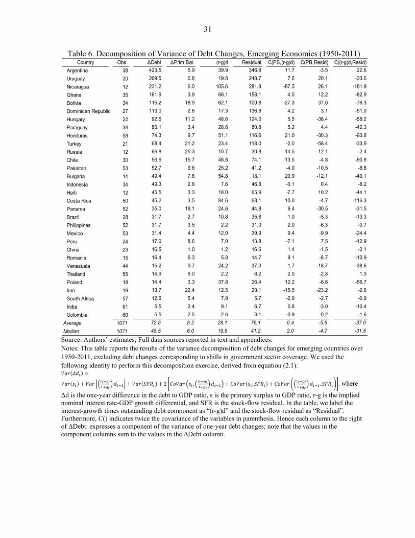
31

Table 6. Decomposition of Variance of Debt Changes, Emerging Economies (1950-2011)

Source: Authors’ estimates; Full data sources reported in text and appendices. Notes: This table reports the results of the variance decomposition of debt changes for emerging countries over 1950-2011, excluding debt changes corresponding to shifts in government sector coverage. We used the following identity to perform this decomposition exercise, derived from equation (2.1):

2 , , , , where

Δd is the one-year difference in the debt to GDP ratio, s is the primary surplus to GDP ratio, r-g is the implied nominal interest rate-GDP growth differential, and SFR is the stock-flow residual. In the table, we label the interest-growth times outstanding debt component as “(r-g)d” and the stock-flow residual as “Residual”. Furthermore, C() indicates twice the covariance of the variables in parenthesis. Hence each column to the right of ΔDebt expresses a component of the variance of one-year debt changes; note that the values in the component columns sum to the values in the ΔDebt column.

Country Obs. ∆Debt ∆Prim.Bal. (r-g)d Residual C(PB,(r-g)d) C(PB,Resid) C((r-g)d,Resid)

Argentina 38 423.5 5.9 39.9 346.8 11.7 -3.5 22.6

Uruguay 20 269.5 6.8 19.8 248.7 7.6 20.1 -33.6

Nicaragua 12 231.2 6.0 105.6 281.8 -87.5 26.1 -181.9

Ghana 35 161.9 3.9 66.1 158.1 4.5 12.2 -82.9

Bolivia 34 115.2 18.9 62.1 100.8 -27.3 37.0 -76.3

Dominican Republic 27 113.0 2.6 17.3 136.8 4.2 3.1 -51.0

Hungary 22 92.6 11.2 48.6 124.0 5.5 -38.4 -58.2

Paraguay 38 80.1 3.4 28.6 80.8 5.2 4.4 -42.3

Honduras 58 74.3 9.7 51.1 116.6 21.0 -30.3 -93.8

Turkey 21 68.4 21.2 23.4 118.0 -2.0 -58.4 -33.9

Russia 12 66.8 25.3 10.7 30.8 14.5 -12.1 -2.4

Chile 30 56.6 15.7 48.8 74.1 13.5 -4.8 -90.8

Pakistan 53 52.7 9.6 25.2 41.2 -4.0 -10.5 -8.8

Bulgaria 14 49.4 7.8 54.8 18.1 20.9 -12.1 -40.1

Indonesia 34 49.3 2.8 7.6 46.8 -0.1 0.4 -8.2

Haiti 12 45.5 3.3 18.0 65.9 -7.7 10.2 -44.1

Costa Rica 50 45.2 3.5 84.6 68.1 10.0 -4.7 -116.3

Panama 52 35.0 18.1 24.6 44.8 9.4 -30.5 -31.5

Brazil 28 31.7 2.7 10.8 35.8 1.0 -5.3 -13.3

Philippines 52 31.7 3.5 2.2 31.0 2.0 -6.3 -0.7

Mexico 53 31.4 4.4 12.0 39.9 9.4 -9.9 -24.4

Peru 24 17.0 8.6 7.0 13.8 -7.1 7.5 -12.9

China 23 16.5 1.0 1.2 16.6 1.4 -1.5 -2.1

Romania 15 16.4 6.3 5.8 14.7 9.1 -8.7 -10.9

Venezuela 44 15.2 9.7 24.2 37.0 1.7 -18.7 -38.6

Thailand 55 14.9 6.0 2.2 6.2 2.0 -2.8 1.3

Poland 18 14.4 3.3 37.8 26.4 12.2 -8.6 -56.7

Iran 19 13.7 22.4 12.5 20.1 -15.5 -23.2 -2.6

South Africa 57 12.6 5.4 7.9 5.7 -2.9 -2.7 -0.9

India 61 5.5 2.4 9.1 6.7 0.8 -3.0 -10.4

Colombia 60 5.5 2.5 2.6 3.1 -0.9 -0.2 -1.6

Average 1071 72.8 8.2 28.1 76.1 0.4 -5.6 -37.0

Median 1071 45.5 6.0 19.8 41.2 2.0 -4.7 -31.5

32

Table 7. Bohn (1998) Test for Fiscal Policy Sustainability

Source: Authors’ estimates; Full data sources reported in text and appendices. Notes: OLS estimation, robust standard errors. Debt coefficients reported; output gap and temporary spending controls included for all countries. Commodity price controls included for relevant countries based on latest WEO list of historical commodity exporters (index which includes oil prices applied to countries dependent on oil revenues). Default years and significant war years excluded; we report results for all countries with at least 25 non-default, non-war observations The number of observations reported refers to the full sample estimation.

Country N

Sweden 0.038*** 0.010 0.085*** 0.084*** 202

United States - 0.006 0.042*** - 0.012 0.064*** 177

United Kingdom 0.043*** 0.005 0.016*** 0.017*** 160

Canada 0.056*** 0.077*** 0.077*** 0.087*** 134

Spain 0.038*** 0.069*** 0.032* 0.054*** 133

Japan - 0.026*** - 0.055*** - 0.03*** - 0.027*** 125

Norway 0.268*** 0.028*** 0.308*** 0.283*** 124

Denmark 0.077*** 0.035*** 0.055*** 0.056*** 123

Italy 0.056*** 0.019*** 0.055*** 0.057*** 118

Portugal 0.031** 0.194*** 0.020 0.047*** 117

India 0.024 0.072*** 0.041*** 0.047*** 99

France 0.037*** 0.017** - 0.042*** - 0.036*** 98

Belgium 0.035*** 0.056*** 0.074*** 0.074*** 97

Netherlands 0.027*** - 0.03*** 0.023*** 0.022*** 97

New Zealand 0.016*** 0.049* 0.005 - 0.014 96

Australia 0.026** 0.035*** 0.033* 0.023 95

Germany 0.023* 0.012 0.028*** 0.03*** 91

Finland 0.049* 0.031 0.035 82

Argentina 0.021 0.010 - 0.006 - 0.011 80

Switzerland 0.017** 0.003 - 0.002 76

Ireland 0.062*** 0.069*** 0.056*** 75

Colombia 0.032 0.026** 0.036 0.042 75

Greece 0.037*** 0.016*** 0.035*** 0.05*** 70

Venezuela 0.008 0.007 0.033 67

Mexico 0.035*** 0.038*** 0.047*** 63

Iceland 0.012 0.034** 62

Austria 0.005 0.009 59

Philippines 0.092*** 0.093*** 57

Thailand 0.003 0.005 56

South Africa 0.040 0.041 54

Korea 0.149*** 0.148*** 53

Pakistan 0.031** 0.029* 53

Panama 0.022 0.025 52

Costa Rica - 0.001 - 0.002 45

Ghana 0.008 0.006 42

Paraguay 0.019 0.029** 41

Turkey 0.19*** 0.193*** 38

Indonesia 0.021 0.018 35

Uruguay 0.035*** 0.035*** 33

Israel - 0.009 - 0.011 32

Honduras - 0.028** - 0.025* 29

Brazil 0.001 0.002 28

Full Sample 1919-2011 1950-2011 1950-2007

33

CountrySignificantly Positive Response

CoefficientSignificantly Negative Response Coefficient

Change to Positive Change from PositivePercent Positive

Percent Negative

Number of Windows

First Window

Sweden 1838, 1841-8, 1853, 1878-1913, 1989-2008

1862-9, 1966, 1982-3 1838, 1841, 1853, 1878, 1989 1839, 1849, 1854, 1914, 2009 49 8 134 1832

United Kingdom 1854-64, 1866-70, 1872-7, 1880-1913, 1978-86, 1990-94, 2003-10

none 1866, 1872, 1880, 1978, 1990, 2003

1865, 1871, 1878, 1987, 1995, 2011

75 0 104 1854

Canada 1926-34, 1966-70, 1994-2011 1973-5 1909, 1926, 1994 1901, 1917,1971 54 3 87 1894Denmark 1904-1911, 1986-2011 1974, 1982 1986 1912 40 2 84 1904Norway 1914-6, 1930-43, 1984-90,

2004-111905-6, 1967-70 1914, 1930, 1984, 2004 1917, 1991 38 7 84 1905

Spain 1903-35, 1975-86, 1996-2009 1961-9 1975, 1996 1987, 2010 70 11 84 1903Japan 1906-33, 1988-96 1902-3, 1939-41, 1976-81,

2002-111906, 1988 1934, 1997 45 26 82 1899

United States 1825-6, 1829, 1904-14, 1968-85, 1996-2008

1990 1829, 1840, 1996 1827, 1830, 1915, 1986, 2009 63 1 73 1825

Portugal 1952-61, 1987-2005 1939-44, 2010 1952, 1987 1962, 2006 40 10 73 1939New Zealand 1952-68, 1979-93 none 1979 1969, 1994 53 0 60 1952France 1904-17 1967-98, 2007-10 none none 24 61 59 1904Belgium 1977-8, 1985-2007, 2009-11 none 1977, 1985, 2009 1979, 2008 49 0 57 1904Netherlands 1904-17, 1969-72, 1975-6,

2000-111984 1975, 2000 1973, 1977 56 2 57 1904

Italy 1906-13, 1993-2011 1973-88 1906, 1993 none 49 29 55 1904Ireland 1989-2011 none 1989 none 42 0 55 1957Germany 1904-6, 1917, 1987-90, 1999-

2011none 1917, 1987, 1999 1907, 1991 40 0 52 1904

Australia 1937-42, 1983-7, 1996-2002, 2004-2011

none 1983, 1996, 2004 1988, 2003 50 0 52 1937

Colombia 1985-9, 1992-97, 1999-2010 1965-80 1985, 1992, 1999 1990, 1998, 2011 49 34 47 1965Switzerland 1966-74, 1985-91 1995-9 1985 1975, 1992 35 11 46 1966Finland none 1976-84, 1993-2002 none none 0 44 43 1969Austria 1973-5 1983-6, 1988-91 none 1976 8 21 39 1973India 1934-45, 1948-57, 1997-1999,

2002-9none 1948, 2002 1946, 2000, 2010 85 0 39 1934

Iceland 1985, 1992 1976-9 1985, 1992 1986, 1993 5 11 38 1974Thailand 1989-90 1978-82 1989 1991 6 14 35 1977Philippines 1979-05, 2011 none 1979, 2011 2006 82 0 34 1978Panama 1989-90 1982 1989 1991 6 3 32 1980Argentina 1920-8, 1933-5 1942-9 1933 1923, 1936 39 26 31 1920Korea 1985-91 1996-2000 1985 1992 23 17 30 1982Greece 1994-2010 1985-6, 1988-90 1994 none 65 19 26 1985Mexico 1963-5, 1971-2, 1978-81, 2011 none 1971, 1978 1966, 1973 50 0 20 1963

Paraguay none none none none 0 0 18 1994Pakistan 1996-08 none 1996 2009 72 0 18 1991Venezuela none 1981 none none 0 7 14 1969South Africa none none none none 0 0 11 1974Israel none none none none 0 0 10 2002Ghana 2011 none 2011 none 20 0 5 2007Honduras none 1978-80 none none 0 75 4 1977Chile none none none none 0 0 1 2011Costa Rica none none none none 0 0 1 2011Indonesia none none none none 0 0 1 1996Average 35 11 45Median 40 3 41

Table 8. Bohn Regression Results Iterated Over Twenty-Five Year Rolling Windows

Source: Authors’ estimates; Full data sources reported in text and appendices. Notes: OLS estimations of equation (3.1), with robust standard errors: . We include in output and expenditure gap controls, and, where applicable, a world commodity price index that includes or excludes oil as appropriate. We consider only 25 year periods that are complete with data, and do not include significant war or default episodes. Dates listed refer to the final year of the corresponding 25 year window: hence 1990-1 refers to the 1966-1990 and 1967-1991 windows. The first column thus reports all 25-year windows for which is positive and significant (at the 5 percent level), and the second column reports all windows in which is negative and significant. The “change to positive” column reports 25-year windows in which becomes significantly positive after not being so in the window immediately prior; the “change from positive” column reports windows in which is no longer significantly positive after being so in the window immediately prior.

34

Table 9. Bohn (1998) Fiscal Reaction Function with Expanding Sample

Source: Authors’ estimates; Full data sources reported in text and appendices.

Notes: Iterative Bohn (1998) OLS regressions of s d Zt t t t , with d t the beginning of period debt ratio,

st the primary balance, and Zt controls for cyclical and other factors, beginning 1950 with twenty-five

observations, expanding by one observation, and excluding countries with postwar defaults. The dates listed correspond to the final year of the subsample. The India window starts in 1978, the year after its last default.

Country Significantly Positive Significantly Negative Postwar Obs.

Australia 1976-2002 none 62

Belgium 1988-2011 none 62

Canada 1996-2011 1974-5 62

Colombia none 1974-2000 62

Finland none 1979-85, 1993-5 62

France none 1974-2011 62

Iceland 2007-8 1978-9 62

Ireland 1988-2011 none 62

Italy 1974-91, 1997-2011 none 62

Netherlands 1983-2011 none 62

New Zealand 1980-95 none 62

Norway 1983, 1992-2011 none 62

Portugal 1990-2008 1981 62

Spain 1977-2010 none 62

Sweden 1989-91, 1996-2011 none 62

Switzerland 1974-5 none 62

United Kingdom 1981-2011 none 62

United States 1974-2008 none 62

Austria 1974-5 none 59

Japan 1990-4 1976-83, 2002-11 59

Denmark 1986-2011 1974, 1982 58

Germany 1989-90, 1994, 2000-11 1981 58

Philippines 1979-2011 none 57

Thailand none 1978-83 56

Korea 1986-1992, 2005-11 none 53

Pakistan 1976-94 2005-11 53

Greece 1994-2010 1985-6, 1988-90 46

India 2003-11 none 35

Israel none none 32

35

Table 10. Structural Breaks in Bohn (1998) Sustainability Test, Post-War

Source: Authors’ estimates; Full data sources reported in text and appendices. Notes: The table presents Bai and Perron (1998) tests for unknown number and location of potential structural

breaks, in the post WWII period, on the Bohn (1998) test, s d d Zt t t t t t , for up to three potential

structural breaks. The country, number and years of breaks are reported in the first four columns, and estimates for ̂ across the subsamples are reported in the next three, with the number of observations and sample years in the last two columns. Venezuela’s sample excludes 1980-87.

Min. Obs. 20 Min. Observations 25% of Sample

Break Breaks Years N Sample

Australia 1985 2 1965 1985 -- 0.078* 0.097*** 0.082** 58 1950-2007

Belgium 1970 2 1963 1989 -- - 0.249* 0.029*** 0.052 58 1950-2007

Canada 1975 2 1974 1993 -- - 0.06** 0.035* 0.247*** 58 1950-2007

Colombia 1975 1 1975 -- -- - 0.169*** 0.102*** 58 1950-2007

Finland 1974 2 1974 1990 -- 0.000 0.064 0.012 58 1950-2007

France 1977 1 1977 -- -- - 0.157*** - 0.032** 58 1950-2007

Iceland 1987 3 1965 1979 1993 0.044 - 0.143** - 0.051 - 0.163*** 58 1950-2007

Ireland 1987 2 1973 1989 -- - 0.012 0.11*** 0.045*** 58 1950-2007

Italy 1974 2 1970 1990 -- 0.118 0.023 0.217*** 58 1950-2007

Netherlands -- 1 1990 -- -- 0.016** 0.143*** 58 1950-2007

New Zealand 1987 2 1973 1988 -- 0.013* - 0.069 0.044 58 1950-2007

Norway 1979 3 1963 1979 1993 - 0.069** 0.058* 0.027 0.088 58 1950-2007

Portugal 1971 2 1971 1993 -- 0.047 0.177*** - 0.026 58 1950-2007

Spain 1977 2 1977 1993 -- 0.024* 0.059*** - 0.006 58 1950-2007

Sweden 1977 2 1977 1993 -- 0.025 0.171*** 0.069 58 1950-2007

Switzerland 1977 2 1964 1978 -- 0.018 0.018* - 0.020 58 1950-2007

United Kingdom 1980 2 1968 1985 -- 0.016 0.133*** 0.267*** 58 1950-2007

United States 1974 2 1974 1993 -- 0.062*** 0.021 0.117*** 58 1950-2007

Austria 1974 1 1974 -- -- 0.474*** 0.017 54 1954-2007

Denmark 1974 2 1974 1989 -- - 0.151** 0.083* 0.030 54 1954-2007

Japan 1981 2 1975 1992 -- - 0.072 0.098*** - 0.036*** 54 1954-2007

Germany 1974 1 1967 -- -- - 0.919** 0.038*** 53 1955-2007

Phillipines 1974 2 1974 1990 -- - 0.152 0.027 0.080 53 1955-2007

Thailand -- 2 1980 1993 -- - 0.088* - 0.053 - 0.010 52 1953-2007

Korea 1978 2 1975 1987 -- - 0.322*** 0.322 0.035 49 1959-2007

India -- 2 1980 1995 -- 0.017 0.031*** 0.158** 48 1950-2007

Mexico -- 0 -- -- -- 0.048*** 48 1950-2007

Pakistan 1977 2 1964 1988 - 0.409*** - 0.031* 0.058 48 1952-2007

Panama -- 1 1989 -- -- 0.037*** - 0.032 48 1956-2007

South Africa 1976 1 1992 -- -- 0.002 - 0.056 47 1950-2007

Greece 1986 1 1990 -- -- - 0.055*** 0.044 42 1966-2007

Venezuela -- 0 -- -- -- 0.019 42 1950-2007

Argentina -- 2 1968 1976 -- - 0.544* - 0.093 0.05*** 25 1950-2000

Country Estimated Debt Coefficients

36

Table 11. Structural Breaks in Bohn (1998) Sustainability Test, Full Sample

Source: Authors’ estimates; Full data sources reported in text and appendices. Notes: The table presents Bai and Perron (1998) tests for unknown number and location of potential structural

breaks, in the entire sample, on the Bohn (1998) test, s d d Zt t t t t t , for up to three potential

structural breaks. The country, number and years of breaks are reported in the first four columns, and estimates for ̂ across the subsamples are reported in the next three, with the number of observations and sample years in

the last two columns.

Country Breaks Years Obs. SampleSweden 2 1852 1972 -- 0.072 0.016** 0.141*** 198 1801-2011

United States 3 1830 1931 1984 0.157*** 0.076*** 0.09*** - 0.073 171 1801-2011

United Kingdom 3 1867 1931 1986 0.046*** 0.065*** 0.031*** 0.055 158 1830-2011

Canada 3 1908 1933 1984 0.042** 0.12*** 0.057*** 0.164*** 132 1871-2011

Spain 2 1935 1972 -- 0.027*** - 0.053*** 0.071*** 131 1869-2011

Norway 3 1913 1939 1979 0.009 0.189*** - 0.056 0.266*** 124 1881-2011

Japan 2 1938 1981 -- 0.024*** - 0.068*** - 0.055*** 124 1876-2011

Denmark 1 1970 -- -- 0.025 0.047*** 123 1881-2011

Portugal 2 1921 1967 -- 0.111 - 0.016 0.076*** 116 1880-2011

Italy 3 1904 1936 1971 0.009 0.004 - 0.041 0.121*** 115 1880-2011

France 2 1913 1977 -- 0.044*** - 0.165*** - 0.032** 98 1881-2011

Belgium 2 1957 1989 -- - 0.006 0.026*** 0.074*** 97 1880-2011

Netherlands 3 1950 1970 1990 0.04*** 0.031** - 0.011 0.142*** 97 1880-2011

India 3 1929 1957 1990 0.031** 0.113*** 0.135 - 0.012 96 1884-2011

New Zealand 2 1969 1989 -- 0.018*** 0.055* 0.125*** 95 1913-2011

Australia 2 1949 1982 -- 0.09*** 0.078** 0.138*** 93 1913-2011

Germany 1 1968 -- -- 0.099*** 0.03*** 90 1880-2011

Finland 2 1968 1988 -- 0.096*** - 0.079 0.031* 81 1921-2011

Switzerland 0 -- -- -- 0.017** 75 1930-2011

Ireland 1 1987 -- -- - 0.005 0.081*** 75 1937-2011

Argentina 2 1931 1967 -- 0.023* 0.072 - 0.014 75 1900-200

Colombia 1 1975 -- -- - 0.124*** 0.097*** 74 1800-2011

Greece 1 1991 -- -- 0.04*** - 0.055** 69 1885-2011

Venezuela 0 -- -- -- 0.007 64 1921-2011

Iceland 1 1990 -- -- 0.008 - 0.024 62 1950-2011

Mexico 1 1962 -- -- 0.059*** 0.054*** 61 1925-2011

Austria 1 1974 -- -- 0.474*** 0.015 58 1954-2011

Phillipines 1 1976 -- -- - 0.607* 0.06*** 57 1955-2011

Korea 1 1978 -- -- - 0.134 0.010 53 1800-2011

Thailand 0 -- -- -- 0.029 53 1953-2011

Panama 0 -- -- -- 0.053*** 52 1956-2011

Pakistan 1 1988 -- -- - 0.084*** 0.063** 52 1950-2011

South Africa 1 1983 -- -- 0.022 0.144** 51 1950-2011

Estimated Debt Coefficients

37

Table 12. Influential Years in Recursive Bohn (1998) Test

Source: Authors’ estimates; Full data sources reported in text and appendices. Notes: Years resulting from searching OLS regressions of s d Zt t t t —with d t the beginning of period

debt, st the primary balance, and Zt controls for cyclical and other factors, from 1800-2011 and excluding war

and defaults—for years that cause ̂ to become insignificant when estimates yield significant ˆ 0 (and analogous for ˆ 0 /insignificant). Blue (tan) denotes influential prudence (profligacy); Bold (non-bold) indicates designation as an influential observation in the initial (secondary) stage of the program. Asterisks denote significance at the 10, 5, and 1 percent levels, respectively.

Country Influential Years N Original EstimateSweden 1803, 1981-2-3-4, 1987-8-9, 1993-4-5, 1996-2000-1, 2006-7 202 0.038***United States 1936-7, 1939, 1941, 1948-49-50-51, 1959, 1975, 1983-7-8, 1990-3, 1998-

2000, 2003-4-5, 2008-11177 -0.006

United Kingdom 1830-46, 1847-8, 1850, 1854-6, 1860, 1900-2, 1906-07-13, 1923-31, 1948-49-50-51, 1952-3, 1954, 1956-7-8-9, 1963, 1981, 1992-4, 2002-3-4-5, 2005, 2009

160 0.043***

Canada 1881-2, 1885, 1891, 1906, 1909-15, 1916-7, 1918-9, 1932-3, 1937-9, 1946-8, 1994-2003, 2010

134 0.056***

Spain 1868-70, 1872, 1875-6, 1883, 1894-5, 1896-1910, 1913, 1915, 1943-4-5, 1976-7, 1978-85, 2010

133 0.038***

Japan 1907, 1939-41, 1960-1-2, 1970, 1985-7, 1988-91-2, 1994, 1995-2011 125 -0.026***Norway 1890-3, 1899, 1915-6, 1927-8-9, 1931-5, 1947-8-9, 1971-4, 1975-7, 1978-82-

83, 1987, 1994-5-6-7, 2000-11124 0.268***

Denmark 1971-2-3-4, 1984-91, 1994-5, 1996-2001, 2005 123 0.077***Italy 1880, 1882-91-92, 1893-6-7, 1898-1903, 1905, 1921-2, 1923-5, 1928, 1935-6,

1939, 1947-9, 1975, 1992-4, 1995-2001-2, 2007, 2011118 0.056***

Portugal 1880, 1922, 1968-70, 1971-8, 1979-81, 2009-10 117 0.031**India 1921-2, 1929-30-31-32, 1945, 1980, 1982, 1983-6, 1989-90, 2007, 2010-1 99 0.024France 1881-8, 1892, 1893-1901, 1909, 1912-3, 1947, 1973-4, 2009-10-11 98 0.037***Belgium 1950, 1980-1-2-3-4, 1989-90-91, 1994-2001-2, 2009-11 97 0.035***Netherlands 1880, 1886-7, 1889-90, 1892-6, 1897-8, 1900, 1903-4, 1908-9, 1911-13, 1949,

1950, 1951-2-3, 1976, 1978-81, 1993-4, 1996, 2000, 2002-3, 2005, 2007-897 0.027***

New Zealand 1917-8-9, 1921, 1931, 1933-5, 1976, 1982-3-4-5, 1995-6, 2003, 2004-6-7, 96 0.016***

Australia 1931-4-5, 1942, 1947-49, 1950, 1960, 2003, 2005-7 95 0.026**Germany 1913, 1958, 1966-7-8, 1975, 1995, 2000, 2002-4, 2007-8, 2010-11 91 0.023*Finland 1976-7-8, 1994-5, 1997-8-9, 2000-1-2, 2006-7 82 0.049*Argentina 1900-1, 1903, 1967, 1969-70-71-72, 1974-5, 2006 80 0.021Switzerland 1946-8, 1960, 1964, 1966-8, 1997, 2003-4, 2007 76 0.017**Ireland 1937, 1960, 1979-83, 1985-6-7, 1988-91, 1992-3, 1997, 2006, 2009-10-11 75 0.062***Colombia 1906, 1931, 1953-4-5-6, 1974, 2003-4-5-6-7-8, 2010-11 75 0.032Greece 1885-6-7-8, 1889-1908, 1911, 1966, 1973-4, 1979-80-81-82, 1993, 1994-8,

1999, 2000-1-2, 2004, 2007-8-9-1070 0.037***

Venezuela 1957, 1979, 1989, 1991-2-3-4, 1999-2000, 2003, 2007-8, 2009-11 67 0.008Mexico 1925, 1949, 1952, 1959, 1961-2, 1964-5, 1978-79-80, 1991-2, 1996-7, 2006,

2008, 2009-1163 0.035***

Iceland 1958-60, 1968, 1974-5, 1984, 1993-4, 1997-8, 1999-2000, 2006-7, 2009-11 62 0.012

Austria 1954-5-6-7-8-9, 1961, 1962, 1964-5-6, 1970-1-2-3-4-5, 1995, 2004, 2009-10 59 0.005Philippines 1960, 1962, 1967-8-9, 1971-2-3-4-5, 1979-80, 1984, 1987-90, 1994-6, 1999,

2001-2, 200957 0.092***

Thailand 1957-9, 1961, 1974, 1975, 1977-8, 1988-9, 1991-2-3-4, 1998, 2003, 2005-6-7 56 0.003South Africa 1950-1, 1952-6, 1964, 1974, 1992, 2007-08-09-10 54 0.040Korea 1960-1-2, 1966-69, 1970, 1990-5, 1996-7, 2009, 2011 53 0.149***Pakistan 1952, 1975, 1978-9, 1987-8, 1990, 1998-9, 2000-3-4 53 0.031**Panama 1965, 1967-8, 1971-2, 1974, 1976-7, 1982, 1987-8-9, 1990-93, 1996 52 0.022Costa Rica 1958-60-61, 1968, 1974, 1978, 1982, 1991-2-3, 2007-08-09-10 45 -0.001Ghana 1971, 1977, 1981, 1983, 1985-6, 1992-3, 1996-7, 2001-2 42 0.008Paraguay 1973, 1974-6, 1977, 1986-7-8-9, 1991, 2003, 2009, 2011 41 0.019Turkey 1971, 1974-5-6, 1980-1, 1986, 1994, 1995-8, 1999-2000, 2002, 2003-7, 2009, 38 0.19***Indonesia 1972-3-4, 1986, 1992, 2001, 2003, 2005 35 0.021Uruguay 1972, 1974-5, 1977, 1982, 1988-9, 1993, 1998-9, 2004-5-6-7 33 0.035***Honduras 1953, 1955-8, 1960, 1962-3, 1965, 1967-74, 1976, 1977-78-79-80, 2011 29 -0.028**Brazil 1981, 1991-2-3-4-5-6, 2002-3-4, 2005-8, 2009-10-11 28 0.001

38

Table 13. Times of Strong Prudence and Profligacy

Source: Authors’ estimates; Full data sources reported in text and appendices.

Notes: Dates of strong prudence are non-war, non-default years that are part of at least one 25 year window with a positive and significant debt response coefficient, that are influentially prudent according to the influential observations routine, and in which the actual primary balance is higher than the forward-looking debt-stabilizing primary balance. Dates of profligacy are non-war, non-default years that are not part of any 25 year window with a positive and significant debt response coefficient, in which the actual primary balance is lower than the forward-looking debt-stabilizing primary balance, and in which at least one of the following is true: i) the year in question is part of at least one 25 year window with a negative and significant debt coefficient, or ii) the year is influentially profligate according to the influential observations routine. The last column reports the total number of non-war, non-default observations for each country. This table reports only countries for which we have at least 30 non-war, non-default observations.

Country Times of Strong Prudence Times of Profligacy NSweden 1987-9, 1996-2001, 2006-7 1915, 1920-2, 1953, 1957 202

United States 1948-51, 1998-2000 1934-6, 2009-11 177

United Kingdom 1830-6, 1841-6, 1850, 1856, 1860, 1906-13, 1954-9, 2002

none 160

Canada 1881, 1891, 1906, 1909-13, 1933, 1937-8, 1946-8, 1995-2003

none 134

Spain 1894-1910, 1913, 1915, 1976-7 1943, 2010 133

Japan 1907, 1985-92 1880, 1997-2011 125

Norway 1915-6, 1927-9, 1931-5, 1971-83, 1987, 1994-7, 2000-11

1881-4 124

Denmark 1984-91, 1994-2001, 2005 none 123

Italy 1882, 1885-6, 1890, 1895-6, 1898, 1900, 1905, 1907, 1909, 1969-80, 1995-2000

1921 118

Portugal 1968-71, 1979 1922, 2006-10 117

India 2007 none 99

France 1881, 1885-8, 1893-6, 1899-1901, 1909, 1912

1948-53, 1978, 1981-4, 1986, 1988-96, 2002-11

98

Belgium 1990, 1994-2002 none 97

Netherlands 1886, 1893-8, 1900, 1903-4, 1908-9, 1911-3, 1949, 1951-3, 1976, 1993-4, 1996, 2002, 2005, 2007-8

none 97

New Zealand 1921, 1933-5, 1976, 1982-5 none 96

Australia 1931-5 none 95

Germany 1967-8, 2000, 2007-8 none 91

Finland none 1952, 1955-6, 1961-5, 1974, 1991-3, 1995

82

Argentina 1900-1, 1903 1937-9, 1949-50 80

Switzerland 1946-8, 1966-8 1992-5, 1997-8 76

Ireland 1987-93, 1997 none 75

Colombia 2003-8 none 75

Greece 1974, 1982, 1993-8, 2000-2 1965, 1969 70

Venezuela none 1958-61, 1969, 1977-8, 1994, 2009

67

Mexico 1978-80, 1991-2, 1996-7, 2006, 2008 none 63

Iceland 1968, 1974-5, 1984 none 62

Austria 1954 1976-80, 1982-3, 1986, 1990-1, 1995, 2004, 2009-10

59

Philippines 1960, 1962, 1967, 1971, 1974, 1979-80, 1984, 1987-90, 1994-6, 1999, 2001-2, 2009

none 57

Thailand 1974, 1988-9 none 56

South Africa none 1964 54

Korea 1970 none 53

Pakistan 1990, 1998-2004 1952-67 53

Panama 1965, 1968, 1971-2, 1974, 1977, 1989 1958-63, 1993 52

Costa Rica none 1963, 1967, 1978-9 45

Ghana 1993, 2001 1983 42

Turkey 1980-1, 1995-8, 2002-7, 2009, 2011 none 38

Indonesia 1986, 2001 none 35

Uruguay 1988, 2004-7 none 33

39

Table 14. Panel Results, Fiscal Response as a Function of Growth and Borrowing Costs

Source: Authors’ estimates; Full data sources reported in text and appendices.

Notes: Six estimations of the primary balance reaction function: 1 2s d g d r d Zt t t t t t t with d t the

beginning of period debt, st the primary balance, gt the unexpected change in the long-term real GDP growth

rate, rt the real sovereign interest rate, and Zt controls for cyclical and other factors, from 1800-2011 (top) and

1950-2011 (bottom). R1 allows only the debt-LT growth surprise interaction term, R2 augments R1 with the HP growth surprise. R3 allows only the debt-LT real interest rate interaction term, and R4 augments R3 with the real LT interest rate. R5 includes both the LT real interest rate and the LT real GDP growth surprise, and R6 augments R5 with the LT real interest rate and change in the LT real GDP growth rate. Asterisks indicate significance at the 10, 5, and 1 percent levels, respectively. The Output Gap, Expenditure Gap, and commodity price indices are abbreviated by Zt,. Country-year indicators for wars where expenditure grew beyond six percent of GDP not shown.

Primary Balance to GDP R2 R3 R4 R5 R6

Full Sample Results

Lagged Debt 0.027*** 0.027*** 0.029*** 0.030*** 0.030*** 0.029***

Debt*Change in HP Growth 0.063 0.179** 0.33 0.861**Change in HP Growth - 13.34 - 51.565*Debt*Real LT Interest Rate 0.067*** 0.049 0.067*** 0.045Real LT Interest Rate 1.859 2.403Output Gap 0.046** 0.031 0.053 0.053 0.084* 0.043Real Expenditure Gap - 0.080*** - 0.081*** - 0.096*** - 0.096*** - 0.093*** - 0.093***Non-fuel Commodity Prices - 0.001 - 0.001 - 0.085*** - 0.088*** - 0.080*** - 0.068***Fuel Commodity Prices - 0.001 - 0.001 (omitted) (omitted) (omitted) (omitted)Constant - 0.632 - 0.605 - 0.688 - 0.729 - 0.737* - 0.720*

Number of Observations 3774 3774 1916 1916 1908 1908Adjusted R-Squared 0.457 0.458 0.558 0.558 0.56 0.565

Postwar (1950-2011) Results

Lagged Debt 0.022** 0.022** 0.015 0.014 0.020* 0.018Debt*Change in HP Growth 0.35 0.359 0.872* 1.238**Change in HP Growth - 0.769 - 26.515Debt*Real LT Interest Rate 0.257*** 0.303*** 0.273*** 0.351***Real LT Interest Rate - 3.235 - 5.432Output Gap 0.173*** 0.172*** 0.241*** 0.240*** 0.308*** 0.291***Real Expenditure Gap - 0.129*** - 0.129*** - 0.273*** - 0.274*** - 0.270*** - 0.270***Non-fuel Commodity Prices - 0.006* - 0.006* - 0.343*** - 0.340*** - 0.345*** - 0.329***Fuel Commodity Prices - 0.002 - 0.002 (omitted) (omitted) (omitted) (omitted)Constant - 0.206 - 0.204 - 0.145 - 0.075 - 0.37 - 0.232

Number of Observations 2394 2394 1219 1219 1212 1212Adjusted R-Squared 0.204 0.203 0.299 0.299 0.313 0.315

R1

40

05

01

001

50p

ct o

f GD

P

05

01

001

50p

ct o

f GD

P

1850 1860 1870 1880 1890 1900 1910 1920 1930 1940 1950 1960 1970 1980 1990 2000 2010year

15th-85th percentile rangemeanmedianGDP-weighted mean

His tory of Debt

-10

-50

5p

ct o

f GD

P

-10

-50

5p

ct o

f GD

P

1850 1860 1870 1880 1890 1900 1910 1920 1930 1940 1950 1960 1970 1980 1990 2000 2010year

15th-85th percentile rangemeanmedianGDP-weighted mean

His tory of Primary Balance

02

04

06

0n

umbe

r of c

ount

ries

02

04

06

0n

umbe

r of c

ount

ries

1850 1860 1870 1880 1890 1900 1910 1920 1930 1940 1950 1960 1970 1980 1990 2000 2010year

Country coverage

Figure 1. Government Debt and Primary Fiscal Balance, 1850−2011, in percent of GDP

Sources: See Data Source Description in main text and accompanying electronic chartbook. Note: The top (middle) panel presents the unweighted and GDP-weighted mean, as well as the median, of the government debt (primary fiscal balance) as a share of GDP for the countries in the sample, whose number at each point in time is indicated by the bars in the bottom panel. The shaded areas show the 15th and 85th percentiles (not shown in the middle panel for the years corresponding to the major wars to preserve readability of the chart).

41

Figure 2. Fiscal Variables (Top Chart) and Rolling Regression Results for Japan, 1875-2011

Notes: In the bottom chart, the value of the blue line in the year 1974 is equal to the debt response coefficient given by the estimate of the Bohn fiscal reaction function over the 25 year period 1950-1974. The value of the red line (right scale) in 1974 is equal to the significance of this estimated debt coefficient. Whenever the blue line is above 0 and the red line is below .05, the debt coefficient for the corresponding 25 year window is positive and significant at the 5 percent level, and hence fiscal policy satisfies the government’s intertemporal budget constraint in accordance with Bohn (1998). Dotted lines indicate the presence of a war or default episode in the corresponding 25 year window.

050

100

150

200

250

perc

ent o

f GD

P

-10

-50

510

15

perc

ent o

f GD

P

1870 1880 1890 1900 1910 1920 1930 1940 1950 1960 1970 1980 1990 2000 2010y ear

Primary surplusDebt (right scale)

0.2

.4.6

.81

p va

lue

-.3

-.2

-.1

0.1

Coe

ffici

ent v

alue

1870 1880 1890 1900 1910 1920 1930 1940 1950 1960 1970 1980 1990 2000 2010ending y ear

Coefficient value

p value (right scale)

42

Figure 3. Periods of Prudence and Profligacy, 1800-2011

-10

-50

510

-.2

0.2

1800 1850 1900 1950 2000

United States

-10

-50

510

0.1

.2.3

1800 1850 1900 1950 2000

United Kingdom

-10

-50

5

-.4

-.2

0.2

.4

1800 1850 1900 1950 2000

Sweden

-50

510

-.05

0.0

5.1

1800 1850 1900 1950 2000

Netherlands

-50

510

-.99

3821

61.

0061

78

1800 1850 1900 1950 2000

Chile

Influentially prudent 25 year rolling Bohn Coefficient, negative and statistically significantInfluentially profligate 25 year rolling Bohn Coefficient, positive and statistically significantStructural Break, full sample tests 25 year rolling Bohn Coefficient, statistically insignificantWar years Forward-looking Policy Maker's criteria>=0 (left scale)Default years Forward-looking Policy Maker's criteria<0 (left scale)

43

Figure 4. Periods of Prudence and Profligacy, 1850-2011

-10

-50

510

-.1

-.05

0.0

5.1

1840 1860 1880 1900 1920 1940 1960 1980 2000 2020

Belgium

-10

-50

510

-.2

0.2

.4

1840 1860 1880 1900 1920 1940 1960 1980 2000 2020

Portugal

-10

-50

510

-.1

0.1

.2.3

1840 1860 1880 1900 1920 1940 1960 1980 2000 2020

Spain

-10

-50

510

-.05

0.0

5.1

1840 1860 1880 1900 1920 1940 1960 1980 2000 2020

New Zealand

-10

-50

510

-.2

0.2

1840 1860 1880 1900 1920 1940 1960 1980 2000 2020

Italy

Influentially prudent 25 year rolling Bohn Coefficient, negative and statistically significantInfluentially profligate 25 year rolling Bohn Coefficient, positive and statistically significantStructural Break, full sample tests 25 year rolling Bohn Coefficient, statistically insignificantWar years Forward-looking Policy Maker's criteria>=0 (left scale)Default years Forward-looking Policy Maker's criteria<0 (left scale)

44

Figure 5. Periods of Prudence and Profligacy, 1850-2011

-10

-50

510

0.1

.2.3

1860 1880 1900 1920 1940 1960 1980 2000 2020

Australia

-10

-50

510

-.2

-.1

0.1

1860 1880 1900 1920 1940 1960 1980 2000 2020

Argentina

-10

-50

510

-.1

0.1

.2

1860 1880 1900 1920 1940 1960 1980 2000 2020

Canada

-10

-50

510

-.2

-.1

0.1

1860 1880 1900 1920 1940 1960 1980 2000 2020

Japan

-50

510

-.05

0.0

5.1

.15

1860 1880 1900 1920 1940 1960 1980 2000 2020

India

Influentially prudent 25 year rolling Bohn Coefficient, negative and statistically significantInfluentially profligate 25 year rolling Bohn Coefficient, positive and statistically significantStructural Break, full sample tests 25 year rolling Bohn Coefficient, statistically insignificantWar years Forward-looking Policy Maker's criteria>=0 (left scale)Default years Forward-looking Policy Maker's criteria<0 (left scale)

45

Figure 6. Periods of Prudence and Profligacy, 1880-2011

-50

5

-.2

-.1

0.1

.2

1880 1900 1920 1940 1960 1980 2000 2020

Denmark

-50

510

-.1

0.1

.2.3

1880 1900 1920 1940 1960 1980 2000 2020

Norway

-10

-50

510

1880 1900 1920 1940 1960 1980 2000 2020

Brazil

-10

-50

5

-.2

-.1

0.1

1880 1900 1920 1940 1960 1980 2000 2020

France

-10

-50

5

0.2

.4.6

1880 1900 1920 1940 1960 1980 2000 2020

Austria

Influentially prudent 25 year rolling Bohn Coefficient, negative and statistically significantInfluentially profligate 25 year rolling Bohn Coefficient, positive and statistically significantStructural Break, full sample tests 25 year rolling Bohn Coefficient, statistically insignificantWar years Forward-looking Policy Maker's criteria>=0 (left scale)Default years Forward-looking Policy Maker's criteria<0 (left scale)

46

Figure 7. Periods of Prudence and Profligacy, 1880-2011

-10

-50

510

-.05

0.0

5.1

.15

1880 1900 1920 1940 1960 1980 2000 2020

Germany

-20

24

68

1880 1900 1920 1940 1960 1980 2000 2020

Peru

-10

-50

510

-.1

-.05

0.0

5.1

1880 1900 1920 1940 1960 1980 2000 2020

Greece

-4-2

02

46

-.2

-.1

0.1

.2

1880 1900 1920 1940 1960 1980 2000 2020

Colombia

-.3

-.2

-.1

0.1

1880 1900 1920 1940 1960 1980 2000 2020

Iceland

Influentially prudent 25 year rolling Bohn Coefficient, negative and statistically significantInfluentially profligate 25 year rolling Bohn Coefficient, positive and statistically significantStructural Break, full sample tests 25 year rolling Bohn Coefficient, statistically insignificantWar years Forward-looking Policy Maker's criteria>=0 (left scale)Default years Forward-looking Policy Maker's criteria<0 (left scale)

47

Figure 8. Periods of Prudence and Profligacy, 1900-2011

-10

-50

5

-.1

-.05

0.0

5

1900 1920 1940 1960 1980 2000 2020

Switzerland

-4-2

02

46

-.02

0.0

2.0

4

1900 1920 1940 1960 1980 2000 2020

South Africa

-50

510

0.0

5.1

.15

1900 1920 1940 1960 1980 2000 2020

Mexico

-10

-50

510

-.6

-.4

-.2

0

1900 1920 1940 1960 1980 2000 2020

Finland

-50

510

-.6

-.4

-.2

0.2

1900 1920 1940 1960 1980 2000 2020

Venezuela, Rep. Bol.

Influentially prudent 25 year rolling Bohn Coefficient, negative and statistically significantInfluentially profligate 25 year rolling Bohn Coefficient, positive and statistically significantStructural Break, full sample tests 25 year rolling Bohn Coefficient, statistically insignificantWar years Forward-looking Policy Maker's criteria>=0 (left scale)Default years Forward-looking Policy Maker's criteria<0 (left scale)

48

Figure 9. Periods of Prudence and Profligacy, 1900-2011

-50

510

-.06

-.05

-.04

-.03

-.02

1920 1930 1940 1950 1960 1970 1980 1990 2000 2010

Honduras

-10

-50

510

-.05

0.0

5.1

.15

1920 1930 1940 1950 1960 1970 1980 1990 2000 2010

Ireland

-10

-50

510

-.1

-.05

0.0

5

1920 1930 1940 1950 1960 1970 1980 1990 2000 2010

Panama

02

46

810

0.1

.2.3

1920 1930 1940 1950 1960 1970 1980 1990 2000 2010

Turkey

-50

510

-.2

-.1

0.1

1920 1930 1940 1950 1960 1970 1980 1990 2000 2010

Thailand

Influentially prudent 25 year rolling Bohn Coefficient, negative and statistically significantInfluentially profligate 25 year rolling Bohn Coefficient, positive and statistically significantStructural Break, full sample tests 25 year rolling Bohn Coefficient, statistically insignificantWar years Forward-looking Policy Maker's criteria>=0 (left scale)Default years Forward-looking Policy Maker's criteria<0 (left scale)

49

Figure 10. Periods of Prudence and Profligacy, 1950-2011

-50

510

-.1

0.1

.2.3

1950 1960 1970 1980 1990 2000 2010

Pakistan

02

46

810

0.1

.2.3

1950 1960 1970 1980 1990 2000 2010

Philippines

-20

24

68

-.2

-.1

0.1

1950 1960 1970 1980 1990 2000 2010

Costa Rica

-10

-50

5

-.2

0.2

.4

1950 1960 1970 1980 1990 2000 2010

Korea

-10

-50

510

-.02

0.0

2.0

4.0

6

1950 1960 1970 1980 1990 2000 2010

Ghana

Influentially prudent 25 year rolling Bohn Coefficient, negative and statistically significantInfluentially profligate 25 year rolling Bohn Coefficient, positive and statistically significantStructural Break, full sample tests 25 year rolling Bohn Coefficient, statistically insignificantWar years Forward-looking Policy Maker's criteria>=0 (left scale)Default years Forward-looking Policy Maker's criteria<0 (left scale)

50

Figure 11. Periods of Prudence and Profligacy, 1960-2011

-50

510

1950 1960 1970 1980 1990 2000 2010

Bolivia

-20

24

68

-.02

-.01

0.0

1

1950 1960 1970 1980 1990 2000 2010

Israel

-20

24

68

-.02

0.0

2

1950 1960 1970 1980 1990 2000 2010

Paraguay

-50

510

.04

.045

.05

.055

1950 1960 1970 1980 1990 2000 2010

Uruguay

02

46

810

-.05

0.0

5

1950 1960 1970 1980 1990 2000 2010

Indonesia

Influentially prudent 25 year rolling Bohn Coefficient, negative and statistically significantInfluentially profligate 25 year rolling Bohn Coefficient, positive and statistically significantStructural Break, full sample tests 25 year rolling Bohn Coefficient, statistically insignificantWar years Forward-looking Policy Maker's criteria>=0 (left scale)Default years Forward-looking Policy Maker's criteria<0 (left scale)

51

REFERENCES Andrews, D. W. K., 1993, "Tests for Parameter Instability and Structural Change with

Unknown Change Point," Econometrica, Vol. 61, No. 4, pp. 821-856. Bai, Jushan and Pierre Perron, 1998, “Estimating and Testing Linear Models with Multiple

Structural Changes,” Econometrica, Vol. 66, No. 1, pp. 47-78. Barro, Robert J., 1979, “On the Determination of Public Debt,” Journal of Political

Economy, Vol. 87, No. 5, pp. 940–971.

Blanchard, Olivier, 1990, “Suggestions for a New Set of Fiscal Indicators,” OECD Department of Economics and Statistics Working Paper No. 90, Paris, France.

Bohn, Henning, 1998, “The Behavior of U.S. Public Debt and Deficits,” Quarterly Journal of Economics, August, Vol. 113, No. 3, pp. 949–963.

Bohn, Henning, 2007, “Are Stationarity and Cointegration Restrictions Really Necessary for the Intertemporal Budget Constraint?” Journal of Monetary Economics, Vol. 54, pp. 1837–1847.

Bohn, Henning, 2008, “The Sustainability of Fiscal Policy in the United States,” in Reinhard

Neck and Jan-Egbert Sturm, eds., Sustainability of Public Debt, MIT Press, Cambridge MA, pp.15–49.

Bordo, Michael, Barry Eichengreen, Daniela Klingebiel, and Maria Soledad Martinez-Peria,

2001, "Is the Crisis Problem Growing More Severe?" Economic Policy, Vol. 16, No. 32, pp. 51-82.

Dincecco, Mark, 2011, Political Transformations and Public Finances: Europe, 1650-1913, Cambridge: Cambridge University Press.

Mauro, Paolo, Nathan Sussman and Yishay Yafeh, 2006, Emerging Markets and Financial

Globalization: Sovereign Bond Spreads in 1870-1913 and Today, New York: Oxford University Press.

Mendoza, Enrique G. and Jonathan D. Ostry, 2008, “International Evidence on Fiscal

Solvency: Is Fiscal Policy ‘Responsible’?” Journal of Monetary Economics, Vol. 55, No. 6, September, pp. 1081–1093.

Reinhart, Carmen M., and Kenneth S. Rogoff, 2009, This Time is Different: Eight Centuries of Financial Folly, Princeton, NJ: Princeton University Press.

52

Reinhart, Carmen M., and Kenneth S. Rogoff, 2011, “From Financial Crash to Debt Crisis,” American Economic Review, Vol. 101, No. 5, August, pp. 1676–1706.

Schularick, Moritz, and Alan M. Taylor, forthcoming, “Credit Booms Gone Bust: Monetary Policy, Leverage Cycles and Financial Crises, 1870–2008,” American Economic Review.