A model for the determination of positions of equilibriumof two rigid bodies which are coupled by means ofpassive elements and points of contactDortmans, L.J.M.G.

Published: 01/01/1986

Document VersionPublisher’s PDF, also known as Version of Record (includes final page, issue and volume numbers)

Please check the document version of this publication:

• A submitted manuscript is the author's version of the article upon submission and before peer-review. There can be important differencesbetween the submitted version and the official published version of record. People interested in the research are advised to contact theauthor for the final version of the publication, or visit the DOI to the publisher's website.• The final author version and the galley proof are versions of the publication after peer review.• The final published version features the final layout of the paper including the volume, issue and page numbers.

Link to publication

General rightsCopyright and moral rights for the publications made accessible in the public portal are retained by the authors and/or other copyright ownersand it is a condition of accessing publications that users recognise and abide by the legal requirements associated with these rights.

• Users may download and print one copy of any publication from the public portal for the purpose of private study or research. • You may not further distribute the material or use it for any profit-making activity or commercial gain • You may freely distribute the URL identifying the publication in the public portal ?

Take down policyIf you believe that this document breaches copyright please contact us providing details, and we will remove access to the work immediatelyand investigate your claim.

Download date: 31. Aug. 2018

-1-

A model for the determination sf positions of equilibrium o4 two rigid bodies which are coupled by means o f passive elements and points of contact.

L. Dortmanc WFW 8 6 -03 5 Translation J. Dietvorst

-2-

Contents

Summary Symbols and operations Reading list Chapter 1: Introduction Chapter 2: The theoretical model

Introduction 2.1. Description of the relative movement of two rigid bodies 2.2. Description of the geometry of rigid bodies 2.3. Conditions for a point of contact 2 . 4 . Prescribed quantities of displacement 2.5. Admissible variations for positions of body A 2 . 6 . Connections between the bodies A and i3 by means of passive

el esnents 2.7. Equilibrium-equations for body A 2.8. The resultant system of equations and the solution-process 2 . 9 . independence of the kinematic and contact conditions 2.10. Matrix notation of the equations 2.11. incremental procedure in case of application to concrete

problems Chapter 3 : Description of the developed software

3.1. Build-up of the programme 3 . 2 . Plain-programme notes

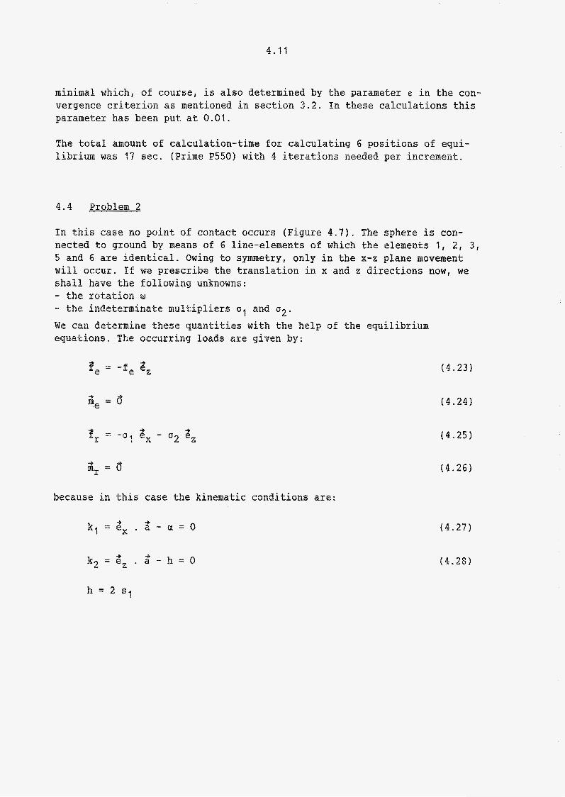
4.1. 4.2. Description of the rotations 4.3. Problem 1 4.4. Problem 2 4.5. Probleira 3 4.6.

Introduction 5.1. Comparison with the Wismans'model 5.2. Possible extensions.

Chapter 4: Come examples Description of the geometry of the sphere and the cylinder

Remaining possibilities of the programme Chapter 5: Possible extensions of the model

- 3 -

Summa r Y

In this report a model is presented that can be used for the determination of positions of equilibrium of two rigid bodies which are coupled by means of passive elements and points o€ contact. The areas of the bodies may be chosen relatively arbitrarily (free from singularities; continuous curvatures). In the model certain movements can be prescribed a priori whereas the coupling of the bodies by means of passive elements is allowed. The resulting system of equations and the resolutions of them by means of a numenical procedure are discussed. The software developed on the basis of this model is explained briefly and some small problems analysed with the help o f this software are discussed. Finally some possible extensions of the model are discussed.

-4-

Symbols

Operations

indices

AC A T

scalar column matrix with scalar components vector column matrix with vector components second order tensor matrix with tensor components rnalrix with scalar components

scalar product or inproduct of two vectors inproduct of A and 6 tensor product or dyadic produet of 2 and 8 vector product of à and 6 length of a vector

conjugate of A transpose of A

-5-

References

1.

2.

3 .

4 .

Veldpaus, F E. : A mathematical joint model (Dutch). Internal report WFW, Eindhoven University of Technology, 1980.

Wicmans, J.C.: A three dimensional mathematical model of the human knee joint. Ph.D. thesis Eindhoven University of Technology, 1980.

Wittenberg, J.: Dynamics of systems o f rigid bodies. B.G. Teubner, Stuttgart, 1977.

Veltkamp, G.W., G @ u ~ ~ s : A.J.: ~ u m e r i c a ~ methods I and PP (Dutch). Course-book Eindhoven University of Technology, nr. 2.211; 1979/1980

1.1

Chapter 1 .

Introduction

During the last few years in the division of Physical and Nechanical Engineering Fundamentals of the Eindhoven University of Technology attention has been paid to the development of a model with which equilibrium positions of the human knee-joint can be detesmined (Wismans [23) . In this model an effort is made to examine in what way the joint takes up its position under the influence of an external load and a prescribed angle of flection. The geometry of the contact surfaces and the ligaments around the knee-joint are also part of this model, with which the ligaments are represented by a number of elastic line-elements. Some objections are attached to this model which was developed by Wismans. The contact surfaces should be described by Deans of two-dimensional polynomials, whereas only the angle of flection can be prescribed. Furthermore, in this model always in two places points of contact are a necessity, which in practice need not be so. An other objection is that for the numerical elaboration of the model many hours of calculation appear to be necessary. In orden to remove a number of these objections Veldpaus C l ] drew up a more general model. Here two rigid bodies are the basis with contact surfaces of which the geometry can be chosen freely. The number of contact points and prescribed ~ove~ents @ay vary, whereas the external loa6 may be a function of the position and the orientation of the bodies, which for example makes it possible to bring in follower forces. This model has been worked out with the exception of the solution of the resulting set of equations, albeit that this model requires the choice of a certain vector base. The movement with respect to this base is described. The model under consideration in this report, in fact is only a further elaboration of the model which was developed by Veldpaus. This elaboration applies to the theoretic substructure of the model on the basis of co-ordinate-free notation and the indication of a method for the resolution of the resulting set of equations. Furthermore, the theory has been used for the development of a computerprogr~~e with which concrete problems can be analysed. The model at issue can be seen as an extension of the Wismans'model. The range of applications of the model can be sought in the mechanics of joints and in the field of technical constructions (cam mechanisms, mul~idimen~ional mass- spring-systems).

Chapter 2.

The theoretical model.

Introduction

In this chapter we shall give information of the way in which positions of equilibrium of the two coupled rigid bodies can be determined. For this pur- pose we shall first mention in what way the relative movement of the two bodies can be described by means of a number of kinematic quantities (section 2 . 1 ) . Then in section 2.2 we shall pay attention to the description of the geometrical quantities which matter in the contact points present, if any. These quantities will come pp fog discussion when in section 2 . 3 we shall speak about the so-called contact conditions. These conditions are conditions which should be satisfied by a contact present between the two bodies. After that in section 2 . 4 we shall discuss the so-called kinematic conditions. With these conditions certain movements can be laid down a priori. In section 2.6 attention will be paid to the connections between the two bodies by means of passive elements. In this model the equilibrium equa- tions should have been satisfied. These are discussed in section 2.7. After that in section 2.8 the total set o% equations will be presented. This con- sists of the contact and kinematic conditions and the equilibrium equations. In general this set is strongly non-linear and cannot be solved analytically. The process of solution presented in section 2.8 therefore is based on a numerical technique, the ~ewton-Raphson method. This method necessitates the derivatives from all kinds of quantities being determined. Therefore, in the sections 2.1 up to and including 2.7 these derivatives are derived, where necessary. This derivation takes place by a study of in- finitesimally small variations of the relevant quantities. After the outline in section 2 . 8 of the process of solution, in section 2.9 we shall show that the set of equations may be singular in case of dependence of the contact and kinematic conditions. For the numerical process of solving it is neces- sary that the vectors and tensors introduced are formulated in terms of their components with respect to some vector-base chosen. The choice of this vector-base in this model is discussed in section 2.10. Finally, in section 2 . 1 1 a discussion takes place on the way in which the model presented may be used for the determination of positions of equilibrium of the bodies for various load values and/or prescribed kinematic quantities.

2 . 1 . Description of the relative movement of two rioid bodies.

In this section we shall examine in what way the relative movement of a rigid body with respect to an other rigid body may be described. For this purpose the rigid body B is assumed to be fixed in space. An ortnogonai co- ordinate system ( x , y, z ) with origin OB and unit-vectors êx, Gy and ez +

2.2

along the respective xf y and z-axes is rigidly fixed to body 8. These vec- tors are stored in a cofuwn matrix sf the vector base fixed in body B:

Here it goes that:

For the rigia body A we apply the same procedure by introducing a rigid or- thogonal co-ordinate systew (a , @, y ) connected with this body, having OA as the origin and unit vectors e,, 2@ ana axes. This time, too, we introduce a column matrix & the orthonormal vector base attached to body A :

-8 along the respective byf p and y-

for which it goes that

E - 3 . ;T= - I (2.5)

The positon of the moving body A with respect to body B can now be laid down with the translation vector a from OB to OAz and the orientation of the (a, B r y ) system with respect to the ( x i y, z ) system. This position is charac- terized by the rotation tensor R, for which it goes that:

R . RC = RC . R = I f 2 . 8 )

Wow we look at the position of a material point P on body A (see figure 2 . 1 1 . The position of this point can be described with the vector 3 from OB to P, whereas this is also possible with the vectors a" and z. In the reference- positions (this is the position at the point of time t=O) the following hold good :

4 .3 Q := r (2.9)

2 . 3

For the vector $ in the momentary position it then goes:

( 2 . 1 1 ) + - 3 g - R . r

With this for the position of the point P in the momentary position it fol- lows that:

( 2 . 1 2 ) 3 f = i i + $ = Z t ~ . r

Now we study the influence of infinitesimally small variations of a' and R. From relation ( 2 . 1 2 ) it follows that:

( 2 . 1 3 1 3 5 3 = ad + QR i r

This can be re-written into:

3 a ? = 634- 6 R . RC . R . r

( 2 . 1 4 ) -v = oa + 6R .RC . Q

As the rotation tensor R is orthogonal the tensor 6R.R' will be skew-sym- metric and have an axial vector 5; such that for each vector 4 it goes that:

With this for relation ( 2 . 1 4 ) i% follows that:

a? = aà .t aft * ; ( 2 . 1 6 )

This relation gives the change of the position vector ? of a point P on body A in case of infinitesimally small changes of the quantities which determine position and orientation of the body A with respect to body 3.

2 . 2 . Description of the aeometrv of the ricrid bodies.

We have assumed that in a number of places contact points may exist for the bodies. In each of these contact points a number of geometrical quantities are of importance, to which we shall pay attention in the Iollowing.

First we shall consider some geometrical quantities of body B. Each point P on the surface of body B can be described with the vector 3 form OB to P. This vector is a function of the spherical co-ordinates x, y and z, so that it goes that

2 . 4

Figure 2.4

Quantities for the description of the relative movement of the rigid bodies A and B.

2 . 5

$ = (x y z ) ( 2 . 1 8 ) I t is required now that the representation 5 -D 6 (5) is unambiguous.

As the point P lies on the surface of body B, a connection between the co- ordinates xI y and z will exist. Therefore, these co-ordinates can be re- placed by t w o surface co-ordinates u and v, for which it goes that:

( 2 . 1 9 )

(2.20)

We require the column g to be an unambiguous function of the column 5. For the point P on the surface of body B it then holds:

Now we study the Fnfuence of i~finit~§~~ally slmall variations of the column y . From relation ( 2 . 2 1 ) it follows that

áC aC aC = au: au 4. E av

Now we define: -* ai! Cu :=

-b a2 cv := ifv

( 2 . 2 2 )

(2.23b)

Here eu and 3, are the tangent vectors to the surface in the point P a t the curves with respectively v=constant and u=constant. These tangent vectors are required t o be i~de~endent. Ihenefore we can introduce the norm1 2 to the surface in the point P:

-9 n" = sn . Cu * eV / ICu * ?,I

2 = 1 n

( 2 . 2 4 )

(2 .259

Here sn is chosen in such a way that the normal 2 is pointing outwards from the body B. As the ~ e q u ~ r ~ ~ e n t has been made that the position vector of the point P shall be an unambiguous function of the co-ordinates 5, and as these co-ordinates will have to be an u*arn~~~ffoff~ function of the co-ordinates g f the value of sn will be the same in every point on the surface of body B.

2 . 6

+ Therefore the vectors Eu, c local vector base in the point P. (see Figure 2.2). To this vector base belongs a reciprocal vector base with base vectors if,, Bv and ifn for which goes that:

and n are independent and are adding up to a Y

is,= EC, 1 + * n"

J v = ? n l - * * Cu

in - E Cu CV - 1 4 * +

+ c = Cu . (Cv * ?i,

With relation (2.24) it follows that:

so that for the vector gn it goes that:

(2.26a)

(2.26b)

(2.26~)

(2.26d)

(2.27)

(2.28)

in case of infinitesimally small variations of the column $ the normal 8 will also change:

(2.29) as a3 on = Ou i- ay ov

For this the vector $(g) must be twice differentiable. With the relations (2.22) and (2.26) we can express the variation 6u and OV in the variation of the position of vector 6". It holds good that:

áv = 8, . o2

Substitution of relation (2.30) in relation (2.29) then yields:

By introduding the gradient operator qS with: a 9s = $u &i + av ay

we can write relation (2.31) as:

(2.30b)

(2.31)

(2.32)

(2.33)

2.7

I

-i I1 -i I1

Figure 2.2

Noraal and tangent vectors for a point i? on the surface of body B.

2 . 8

Bn 8n In appendix A relations are derived from the vetors au and E. It appears to be that:

(2.34)

(2.35)

Now we introduce the normal curvatures of the surface in the point P, ac- cording to:

+ 3Zu Kuu = - au (2.36a)

(2.36b)

$y substituting the relations (2.34), (2.35) and (2.36) in relation ( 2 . 3 1 ) we find that:

For the curvature tensor R therefore, it holds:

K = -(a,G)c

= ~uuf5u~u i- ~ u v ~ u h i- Kvuifvifu KvvBvk (2.39)

Now we suppose that the vector c is twice continuously differentiable. It then goes that:

a;, azv r = a U

or:

Kuv = RVU

In this case the curvature tensor K is symmetric:

(2.48)

(2.41)

2.9

K = KC ( 2 . 4 2 )

For variations of the normal n' it then holds that:

(2.43)

The curvature tensor K is singular because from relation ( 2 . 3 9 ) it follows that :

K . ; = a As the tensor K is symmetric and singular, this tensor has 3 real eigen- values, of which minimally one equals zero. The two remaining eigenvalues are the principal normal curvatures of the surface in the point P. So far some geometrical quantities for body B.

In principle, €or body A similar relations hold good as those for body B. All kinds of quantities which have been determined for body B, can also be determined for body A . In this context it should really be borne in mind that the body A may change its position. In the following sections it will appear that the geometrical quantities for body A need being determined for the position of the body only on the point of time t=O, the initiai position. In future we shall refer to these quantities by the same symbol has been used for these quantities for body B, but then marked with the su- perscript A .

2 . 3 Conditions for points of contact.

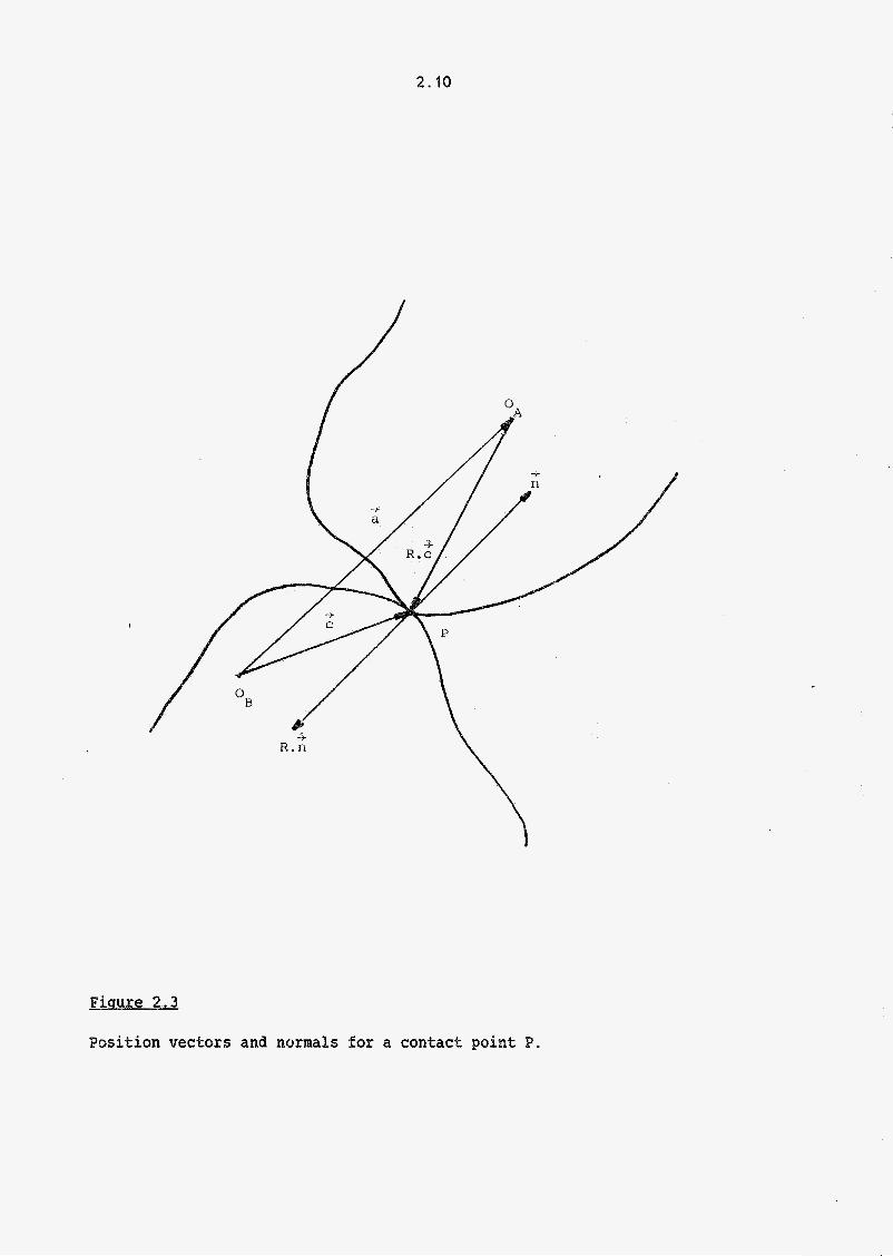
If there is a point of contact for theAbodies A and B such that body's €3 point P coincides with body's A point P, consequently a numbes of conditions arise for the geometrical quantities in these contactpoints as derived in section 2 . 3 . These so-called contact conditions will be discussed in %he following.

With respect to the position of this point, for the point P on the surface of body Is (see Fig. 2 . 3 1 , it holds that

-9 -b r = c(g) P

For the point P on this body it holds

(2.45)

the surface of body A at the instantaneous position of that

12.451

2.10

Fiuure 2.3

Position vectors and normals for a contact point P.

2.11

Should the points P and P coincide, the following must then be the case:

A second condition €or points of*contact is that the normals to the surface are in line at the points P and P.

(2.48) 4 4 n = - R . n

(see Figure 2.3) A

In case of variation of 2, a', R k! etc. it may happen that a point of contact vanishes. Variations which do not take away the point of contact will be denoted as "contact variations"' of the above quantities. From the relations (2.47) and (2.48) for these variations it follows that:

(2.49)

(2.50)

4 62 = 6; + 6if * (R . c) +. R a ei$

6; = - 5 8 * (R . a) - R . 6d

With the help of relation (2.38) it follows that:

63 = -K . 62

6i = -i .

and substitution ofAthes$ relations inarelation (2.50) yields: (2.51) 4 K . ~ C + R . K . a Z = a ï ! * ( R . n)

From relation (2.49) we can now solve either 6; or tic and substitute in relation (2.51). This then yields the relations:

(R i- R . . Rc) . b Z = 68 * (R . $1 +. R . i . RC . 63 ( 2 52 1 (2.53)

(2.54)

As a result of pre-multiplication by 2 from relation ( 2 . 4 9 ) it follows that:

(2.55) d n . 62 = n . (62 i- 6# * (R . c) i- R . 6s)

However, it goes that:

n . & = O -P (2.56)

2.12

1 Z . R . 6 8 = - n . RC . R . bi? = O (2.57)

so that from relation (2.55) it follows that:

Now the relations (2.471, (2.48)‘ (2.521, (2.53) and (2.58) are the contact conditions sought after. Relation (2 .58 ) expresses that in case of variations 152 and 5 8 the vector 62

t 6% * (R.:) must be in the tangent plane to the surface in the contact point. This means that variations 52 and 6 8 ought not make disappear the point of contact. From the relations (2.52) and ( 2 . 5 3 ) variations 5 8 and can be determined for known variations 63 and 6 8 . The magnitude of öb and 5 s Is also determined by the curvatures of the surfaces in the contact point, as can be expected. Were the tensor K t R.K.RC plays an important part. We call this tensor the equivalent curvature tensor of the surfaces in the con- tact point. In appendix B it is demonstrated that this tensor is singular. In appendix B is also mentioned in what way 63 and 158 can be determined from the relations (2.52) and (2.53) despite the singularity of the equivalent curvature tensor.

2.4. Prescribed quantities of disrtlacement.

In general the moving body A has six degrees of freedom viz. the 3 com- ponents of the translational vector in a chosen vector base and 3 rotational parameters with which the rotational tensor R can be described. It Is true that the matrix representation of this tensor in a chosen vector base has 9 components, but owing to the orthogonality of this tensor there are only 3 independent components. Now it may happen that we want to prescribe one or more degrees of freedom or that we want to impose one or more kinematic conditions. Let us now assume that m kinematic conditions having the form

k j ( Z r R) = O j = 1 ... IB (2.59)

are given. These conditions are supposed to be independent. By kinematic variations of a and R, variations which leave the kinematic conditions intact are meant. For these variations it should then hold that:

k j t a + 62, R + 6R) = O j = 1 ... m (2.60)

In general from relation (2.60) a relation having the form:

. 6 a , + i t j . Ft*=o j = 1 ... m (2.61) 4

“ j

2 . 1 3

can be derived. Here the vectors a j and lf nature of the condition kj. In appendix D for a number of cases relation ( 2 . 6 0 ) is further elaborated. In the same appendix, too, attention will be paid in more detail to the parameters by which the rotation tensor R can be described.

are entirely determined by the

2 . 5 . Admissible variations for the position and the orïentation of body A.

In section 2 . 3 the requirement has been made that variations of 3 and R do not make disappear the point of contact, whereas in section 2 . 4 the require- ment has been made that variations of $ and R leave the kinematic conditions intact. Variations of a and R satisfying both requirements are called admis- sable variations. Therefore, these variations satisfy the relations ( 2 . 5 8 ) and (2.611:

k = 1 ... n. With n €or the number of contact points present.

( 2 . 6 2 )

( 2 . 6 3 )

j = 1 ... m. With m for the number of kinematic conditions present.

We have ruled out that all degrees of freedom of body A have been fixed. As each contact point present in fact should be considered a fixed degree of freedom, therefore, the inequality

m + n 1 5

should always be satisfied. By substitution of relation ( 2 . 4 8 ) we can rewrite relation ( 2 . 6 2 ) as:

(R . i,) . aa + (R . (f, * i,,, . a* = o

k = 1 ... n

( 2 . 6 4 )

(2 .651

In section 2.9 we shall consider the relations ( 2 . 6 3 ) and (2.65) in @ore detail. There it will appear that in some cases these relations are not in- dependent, which will turn out to have consequences on the solvability of the set of equations as given in section 2 . 8 .

2.14

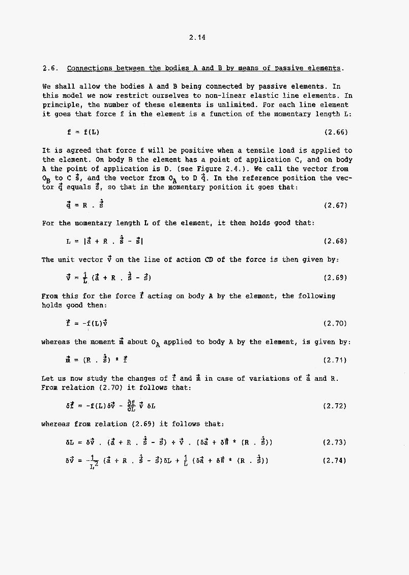
2.6. Connections between the bodies A and B bv means of Passive elements.

We shall allow the bodies A and B being connected by passive elements. In this model we now restrict ourselves to non-lineas: elastic line elements. In principle, the number of these elements is unlimited. For each line element it goes that force f in the element is a function of the momentary length L:

f = f(L) (2.66)

It is agreed that force f will be positive when a tensile load is applied to the element. On body B the element has a point of application e, and on body A the point of application is B. (see Figure 2.4.). We call the vector frox OB to C g, and the vector from OA to D 9. In the reference position the vec- tor 4 equals s , so that in the momentary position it goes that:

-* -3. q = R . s

For the momentary length L of the element, it then holds good that:

(2.67)

(2.68)

The unit vector ? on the line of action CD of the force is then given by:

From this for the force ? acting on body A by the element, the following holds good then:

ip = -f(L)V (2.70)

whereas the moment 4 about OA applied to body A by the element, as given by:

(2.71)

Let us now study the changes of f and 3 in case of variations of 2 and R. Frolit relation (2.70) it Eollows that:

whereas from relation (2.69) it follows that:

1 4 b S = -9 ( 3 t R . s - 8)6L 9 2 ( 6 3 t ai9 * (R . i))

(2.72)

(2.731

(2.74)

2.15

Fiuure 2.4

Connection between the bodies A and B by means of a line element.

2.16

A s the vector f is a unit vector we also have:

f . 6 3 = 0 (2.75a)

or:

Substituting now the relations (2.75) and 12.73) in relation (2.741, it then follows that:

(2.76) 1 -6 03 = L (I - Ga, . ( 6 8 t tiif * (R . s ) )

With this for relation (2.72) it follows that:

6 z = V . ( 6 2 t 68 * (R . $1) ( 2 . 7 7 )

v = (f/L - -&3f - (f/L)I (2.78)

We define a skew-symmetrie tensor C , for which we have:

(2.80) + i C . w = (R . s ) * w' for each 4

With these quantities, for relation (2.77) it follows that:

62 = v . ( 5 2 i- sc . 69) (2.81)

For the change of the moment g, with relation (2.71) it follows that:

63 = (15$ * [R . 3)) * d t (R . 21 * 6? (2.82)

With the relations (2.80) and ( 2 . 8 2 ) and the definition of the skew sym- metric tensor F with:

F . i; = 3 * w" for each (2 .831

for relation ( 2 . 8 2 ) it follows that:

& = S . V . 6 8 t ( F . S t S . V . Cc). 69

2.7. Equilibrium euuations for body A .

( 2 . 8 4 )

On body A a number of loads can be working. As the body should be in equi- librium, six equilibrium equations are given below. The loads which can be working on the body are:

2.17

the external load: force vector 3 -*e - moment vector me.

the load of the line elements: force vector ?l = E: ?j with 1 for the number of line elements (2.85)

1 j = 1

1 i moment vector 2î1 = E: (R . s j ) * Pj j=1

the load resulting from the kinematic conditions:

force vector 3 +r moment vector 5

In the following these loads are further discussed.

(2.86)

the load resulting from the points of contact present: In the contact points a contact force p is working. We take p positive if real contact is made. The force vector p' will be working according t o the normal on the surface, so that it gives for the entire force and moment vector resulting from point contact:

(2.87)

( 2 . 8 8 )

As the body A should be in equilibrium, the sum of the forces and the mo- ments should be zero:

(2.89)

(2.90)

We now make the demand that also in case of infinitesimally small variations of the forces and moments the state of equilibrium remains. Consequently the following should hold:

(2.91)

(2.92)

With the expressions for the forces and the moments which were already men- tioned, we shall elaborate these relations in greater detail. For the variations atl and 6alt with relations (2.81) and (2.84) it gives:

2 .18

1 1 - E vj . aa + * E v j . s; . aa )"I

1 1 am, = E: s j * Vj . O 8 + E:

j=l j = l (Fj . Sj + S j . Vj . S;) . OrF

1 2 1 2 Now we shall define the tensors F1, F1, Ml and H1:

1 Fi := j f l Vj

1 F? := jfl vj . s!j

1 Ml := j f l Sj .

1 := jl;l ( F j . S j + S j . V j . S;)

( 2 . 9 3 )

( 2 . 9 4 )

( 2 . 9 5 )

( 2 . 9 6 )

( 2 . 9 7 )

( 2 . 9 8 )

which has the following consequence for the relations ( 2 . 9 3 ) and ( 2 . 9 4 ) :

óP1 = FI . 68 + F? . 69 ( 2 . 9 9 )

( 2 . looi aml = Mi . 63 + Mf . 6%

For the variations 6?k and aiik, with the relations ( 2 . 8 7 ) and ( 2 . 8 8 ) it follows :

In appendix C these relations are elaborated into:

I 2 1 2 For expressions for the tensors Fkl Fkt Mk and Mk appendix C is referred to.

Now we shall study the variations 6fe and age. In general the external loads can be a function of the position and orientation of the body B r as for ex- ample in the case o f a follower force. Therefore:

2 . 1 9

( 2 . 1 0 5 )

( 2 . 1 0 6 )

Formally the waniations 6?e and 6te are then given by:

( 2 . 1 0 7 )

1 1 2 Here the tensors Fe, F;, Me and He are entirely defined by the relations between ge and se and a and R. in appendix E for a number of cases attention is paid to this. The variations afr and 6Sr are BOW the last ones we shall study. The loads fr and gr must be brought into account because by prescribing one or more kinematic conditions one or more degrees of freedom of the body A are suppressed. In general the suppression of these degrees of freedom can only be achieved by the application of a load on the body A . In general the mag- nitude of 2, and will depend on 2 and R. Therefore:

( 2 I 0 9 )

(2 .1101

ittenburg [ 3 pp. 173-1793 the derivation is found that these loads satisfy :

(2 .911 )

In other words no work is done by these loads. In Wittenb~r~ [ 3 pp 173-1743 the derivation is also found that these loads are given by:

(2 .112 )

(2 .113 )

with m for the number of hinematic conditions. Here the vectors s j and 8 j have already been introduced in section 2.5 . In principle the parameters o j are still unknown. With these relations f o r the variations 152~ and it follows that:

(2 .114 )

( 2 . 1 1 5 )

2.20

In general the vectors 8 j and itj can be a function of d and R. Fornally we then can write for the variations a8j and &ij:

h j .o = Dj 1 . 52 -i- Dj 2 . 68j = Dj 3 . ad + D j 4 . 6 3

(2.116)

(2.117)

In ap enalix D for a number of cases further attention is paid to the tensors , DjP D. and Dj. Besides, the relations (2.116) and (2.117) hold good only !r the I-Zh 'kinematic condition is twice differentiable. We make the demand

that this will always be the case Mow we shall define the tensors F,, F,, &ir and Bir according to:

1 5 3 4

i 2 1 2

1 " I F, = -1 D . D j=t 3 I (2.118a)

4 m RL = --E1 u j Dj

With these tensors it follows that:

1 2 m tsiii, = ,E au* it. -+ pil, . tiai i- w, . sá ]=I 3 7

(2.118b)

(2.11842)

(2. Ilad)

(2.119)

(2.120)

With the derived relations Pn the foregoing text f o r the variations of the loads for the relations (2.91 1 and ( Z . 92) it follows that:

(2.121)

(i. 122)

In order that the equilibrium of body A will not be disturbed, the varia- tions 63' 63, tipk and 6uj should satisfy these six relations.

2.21

2.8. The resultino set of equations and the solutionproces.

In the foregoing sections the equations have been discussed, describing the position and orientation of the body A , whereas the equilibrium equations have also been discussed. The resulting set of equations is as follows:

-? 3 nk = -R . nk k = 'i ... n

These are 5n contact conditions because the normals vectors.

and "n are unit-

These are m kinematic conditions

These axe 6 equilibrium equations.

In total these are 6 t 5n t m equations. As it should always hold that m - < 5, the number of equations can amount to a maximum of 31. The unknowns are : * 3 components of the vector 2 * 3 components of the rotation tensor R * for each contact point the 4 surface parameters u, v, u and v * for each kinematic condition an indefinite multiplier o * for each contact point a contact force p.

In total these are 6 t 5 n t m unknowns which should be defined by the 6

+ n

t 5n 9 m equations. Solving the set of equations with the help of an analyti- cal method will often be impossible because in general they are strongly non-linear. Therefore, in general, solving the set of equations will have to take place through a numerical method. Mere we choose for the Newton-Raphson method. This is an iterative solution process which in principle works as follows : Suppose we have a set of non-linear equations O€ the Iorm:

(2 .123)

in which the column matrix z is a non-linear function of the unknown column 2. The exact solution then satisfies:

2 . 2 2

If we now take an initial estimate zo for which does not differ too much from the exact solution, we can make a correction Agol and make the demand that the following satisfies:

A s then A&-, is small with respect to zo, we may linearize the set of equa- tions about the solution go:

If the matrix haps better solution & f then is the result of:

is regular now, we can define from this relation AZo. A per-

= go + A& ( 2 . 1 2 7 )

We can continue the process outlined abave until in the k-th iteration the column Agk satisfies a certain criterion criterion for example may have the following expression:

This so-called convergence-

l-,l c e ( 2 . 1 2 8 )

In [ 4 ] proof is given that this process is quadratic convergent near the exact soìutiun ij. We shall explain now in what way the solution process outlined can be ap- plied to the equations which were derived earlier. For this purpose the contactconditions are the basis. We define the vectors ijk and fik (k = I ... n):

For the exact solution it therefore holds that:

gk = a It, = 6

k = 1 ... n

k = 1 ... n

2 . 2 3

In the j-th iteration, after linearization of the contact conditions, it then holds that:

( 2 . 1 3 1 )

(2 .132)

( 2 . 1 3 3 )

( 2 . 1 3 4 )

As in this process only linear terms are involved, in good approximation it wil1 hold that:

Quite on the analogy of the relations ( 2 . 5 2 ) and ( 2 . 5 3 ) the relations ( 2 . 1 3 3 ) and ( 2 . 3 3 4 ) can then be rewritten as follows:

( 2 . 1 3 5 )

( 2 . 1 3 6 )

(2 .137)

in the way as described in appendix 3, from this the incremental changes of the surface parameters, Ay and A?, can be determined, if A$ and A# are known. By multiplication of relation ( 2 . 1 3 1 ) by the vector R.gk it follows that:

4 i *{AZ + Ab * (R . Ck) + R . Ask - hzk) ( 2 . 1 3 9 ) -9 (R 8,) . gk = (R - nk) It now holds that:

2 . 2 4

he term tik.h?k is quadratic in the differences and, therefore may be put at zero. Furthermore it holds that:

( 2 . 1 4 1 )

( 2 . 1 4 2 )

ith the relations (2 .140 ) up to and includin~ ( 2 . 1 4 2 ) €or relation (2.130) it Eolfows that:

Mow we shall study the kinematic conditions:

ki(2, R) = O i = 1 ... m In the 9-th iteration will then hold:

ki + Aki = 0

with:

(2 .143 )

( 2 . 1 4 4 )

( 2 . A451

(2 .1461

(compare this with relation ( 2 . 6 1 ) ) .

As the last set of equations the equilibrium equations (2.89) and (2.90) are now left. Here, in the j-th iteration, it holds that:

( 2 . 1 4 7 )

( 2 . 1 4 8 )

FOP the terms Af,, A f l etc., in section 2.7 all relations required have been derived. With these relations it €0110~~ that:

( 2 . 1 4 9 )

2.25

Now we s h a l l define the fo l lowing q u a n t i t i e s :

1 1 1 1

2 2 2 2 F2 = Fe t F1 t F, t Fk

1 1 1 1 M1 = Me 4- M 1 9 Mr i- Mk

2 2 2 2 M2 = Me i- M1 t #, + Mk

F1 = Fe t F1 t F, t Fk

3 = ge 31 + fr + ?k

- 3 9 -9 t 4 m = me t ml t ?ar t mk

APT = CAPI 5P2 - - - 5Pn1

(2.150)

(2 .151a)

(2.151b)

( 2 . 1 5 1 ~ )

(2.151~1)

(2.151e)

(2 .151f)

(2.151g)

(2.151h)

(2.1511)

(2.1513)

(2.151k)

(2.1511)

(2 .151~1)

( 2 . 1 5 1 ~ )

With these q u a n t i t i e s we can write t h e r e l a t i o n s (2.1431, (2 .145) ' (2.149) and (2.150) as fo l lows:

Fa . A a + F 2 . A $ - @ G p - ~ A ~ + f = d (2.152)

€4' . A a t M 2 . 5 $ - f 5 ~ - f 5 g t ~ = d (2.153)

g T . A a t f T e A $ t g = C (2.154)

8' . 5 a t fT . A $ t = 0 (2 .155)

2 . 2 6

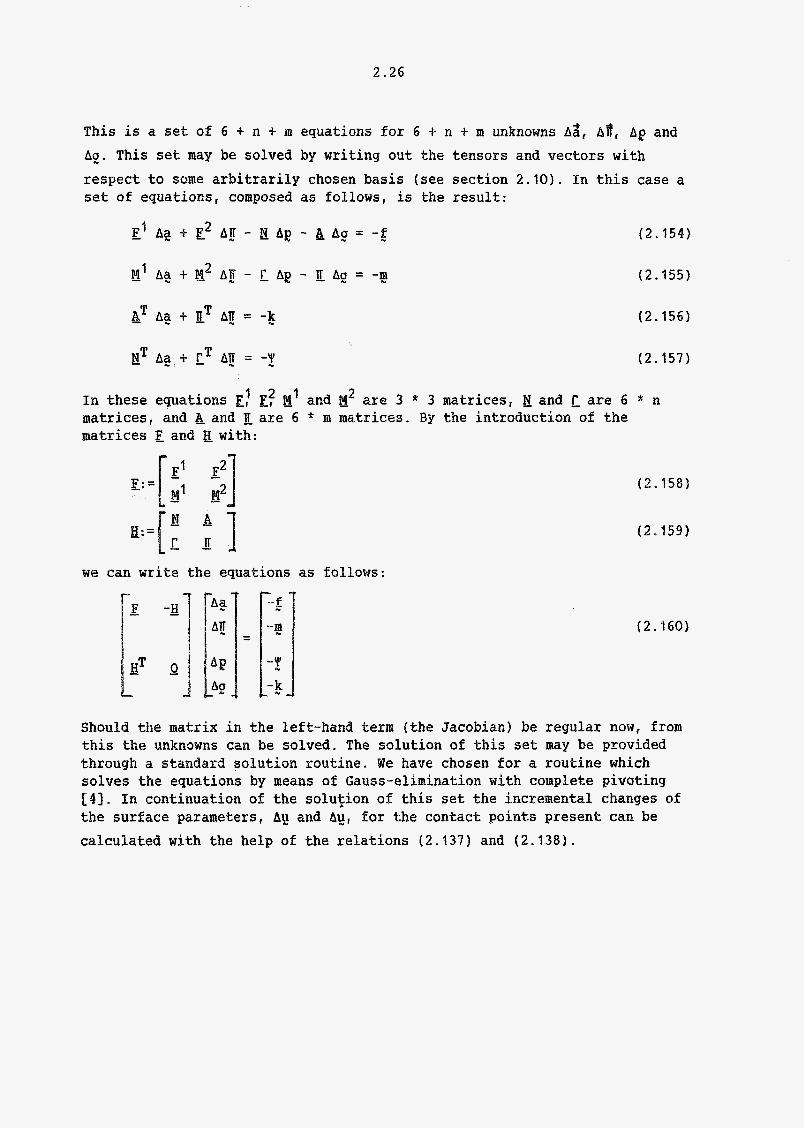
This is a set of 6 + n + m equations for 6 i- n + m unknowns A;, A$, Ap and Ag. This set may be solved by writing out the tensors and vectors with respect to some arbitrarily chosen basis (see section 2 . 1 0 ) . In this case a set of equations, composed as follows, is the result:

( 2 . i 5 4 1

(2 .1551

(2 .156 )

(2 .157 )

1 2 1 2 In these equations E, E, ank M are * 3 matrices, and are 6 * n matrices, and &and E are 6 * m matrices. By the introduction of the matrices and g with:

we can write the equations as follows:

(2 .158 )

(2 .159 )

(2 .160 )

Should the matrix in the left-hand term (the Jacobian) be regular now, from this the unknowns can be solved. The solution of this set may be provided through a standard solution routine. We have chosen for a routine which solves the equations by means of Gauss-elimination with complete pivoting [ 4 ] . In continuation of the solution of this set the incremental changes of the surface parameters, Ag and Aur for the contact points present can be calculated with the help of the relations (2 .137 ) and ( 2 . 1 3 8 ) .

2.27

2.9. Independence of the kinematic and contact conditions.

In section 2.5 the derivation has been made that for admissible variations 68 and 6$ it holds that:

(2.161)

(2.162)

When studying the Jacobian derived in section 2.8 (relation (2.160)), it now appears that this Jacobian is singular if the following has been satisfied:

+ 3 a j = f . n i . nk

aj = f . R cs, * i,, (2.163)

(2.164)

for certain -j and k. Here the factor f is a constant. In this case these contact and kinematic conditions coincide, in other words they are depend- ent. In appendix F this phenomenon is explained with the help of a simple example.

2.10. Matrix notation of the esraation.

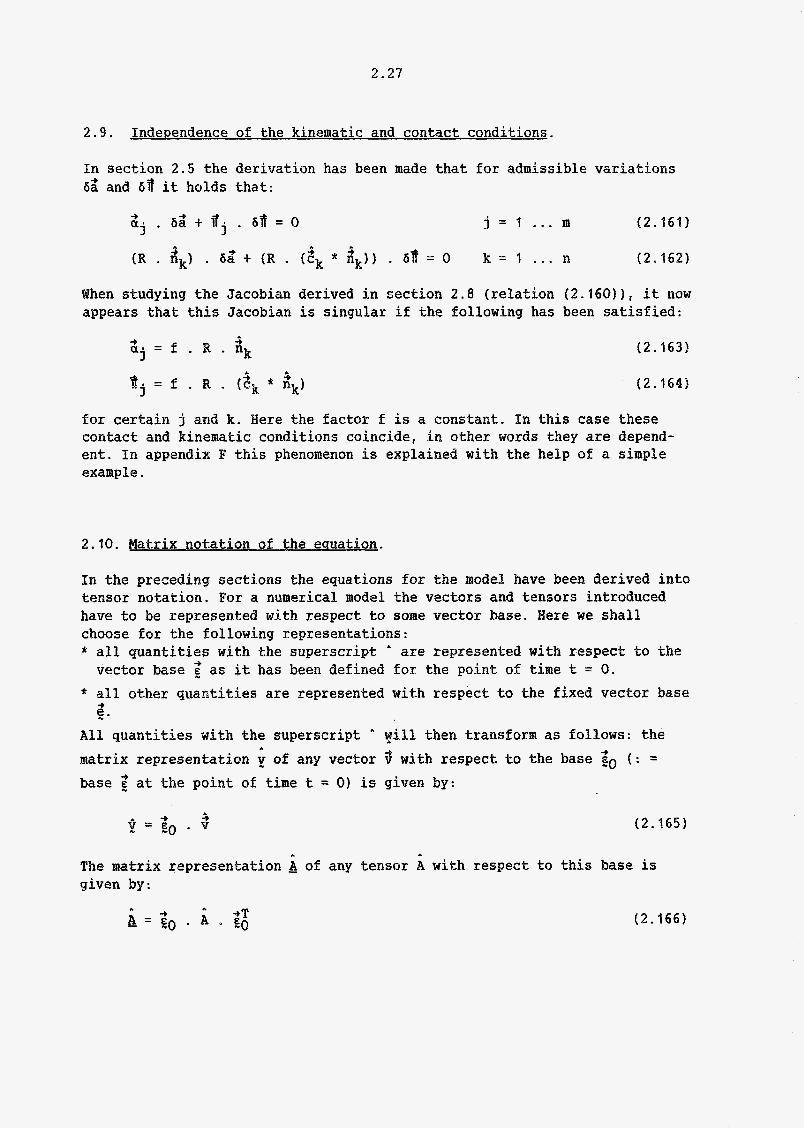
In the preceding sections the equations for the model have been derived into tensor notation. For a numerical model the vectors and tensors introduced have to be represented with respect to some vector base. Here we shall choose for the following representations: * all quantities with the superscript A are represented with respect to the

* all other quantities are represented with respect t o the fixed vector base vector base $ as it has been defined for the point of time t = O.

-# e - All quantities with the superscript &

matrix representation y of any vector base at the point of time t = O ) is

-P 3 p g 0 . v

will then transform as follows: the 3 with respect to the base go ( : =

given by :

(2.165)

A

The matzix representation & of any tensor A with respect to this base is given by:

(2.166)

2.28

For the matrix representation of the remaining quantities quite analogue relations apply.

2 .11 . Incremental Drocedure in case of apalication to concrete Problems.

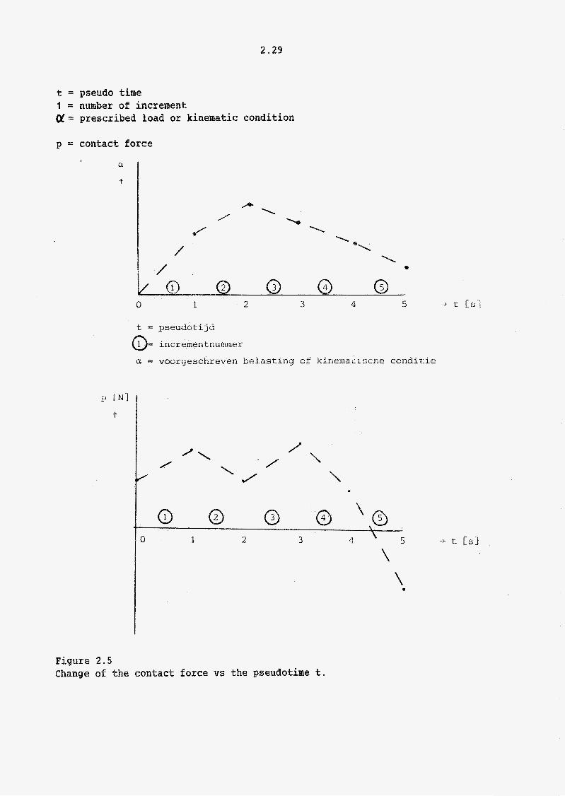
In the foregoing we have described in what way an equilibrium position of body A can be determined in case of given load etc. Now it will often be interesting to know which equilibrium positions occur with several external loads andlor kinematic conditions. In the numerical process based on the preceding theory we can determine these equilibrium positions by repeating this process a number of times with a change in each repetition of the load or the kinematic condition. Hence forth we shall call such a repetition an increment. This incremental procedure now needs a further discussion about a number of things. In the preceding theory the fast has been made use of that the point contact between the bodies A and B was not to be cancelled. With practical problems now it may occur that the contact point is cancelled. In our model this will find expression in the fact that the contact force in a point of contact then becomes negative. Here the question arises in what way we can simulate the cancellation of a point of contact. In order t o be able to answer this question we intxoduce a pseudo-time t, which has been coupled with the num- ber of the increment. As the number of increment has been coupled with the value of a prescribed load or condition, we can also couple the value of the contact force with this pseudo-time (see Figure 2.5). In this example the contact point is cancelled during increment number 5. As in this model we are only considering positions of equilibrium at discrete pseudo-points of time, we can simulate the cancellation of a point of con- tact by repeating increment 5 after the point of contact has been eliminated from the points of contact present. In this way we get no information about the value of u at which the point of contact is cancelled exactly; hovetver, this is irrelevant because positions of equilibrium are only determined at given pseudo-points of time. Apart from that, the moment of cancellation may be determined by adapting the size of the increments (i.e. the change of u during an increment). This will often have to take place afterwards because as a rule it cannot be determined a priori when a point of contact will vanish. To avoid extra cal- culations, therefore in the computer program, which is based on the model presented, a restart option has been included with which the calculation from a certain increment can be continued or repeated.

2 . 2 9

t = pseudo time 1 = number of increment 01 = prescribed load or kinematic condition

p = contact force I

t = pseudotijd

= incrernentnurnmer

cc = voorgeschreven belasting of kinenia,Lsche conditie

\

o O 1 2 3 (i - 5

Figure 2.5 Change of the contact force vs the pseudotime t.

Chapter 3

Description of the software developed

In this chapter we shall discuss the software developed within the framework of the theory which was under consideration in chapter 2. In view of the size o f the program, in this report no ìisting of it has been included; we shall explain, however, in what way the program has been built up roughly and in what way the software can be used for the analysis of a certain problem.

3.1 Build-up of the program.

When developiag the program ax attempt has been made to construct such a build-up of the program that it can be used by any possible users in a rather short time. For this reason a program has been chosen built up of a number of subroutines which are controlled by a main program. In fact this main program then consists o f a number of routine calls and choices f o r the calculations to be made. Now, in the theoretical model a number o f quantities have been introduced which are entirely problem-de~endent, such as the geometry, the properties of the line elements etc. The user should be able to state these quantities. The routines, therefore, can be subdivided into two classes viz. - standard routines - problem routines.

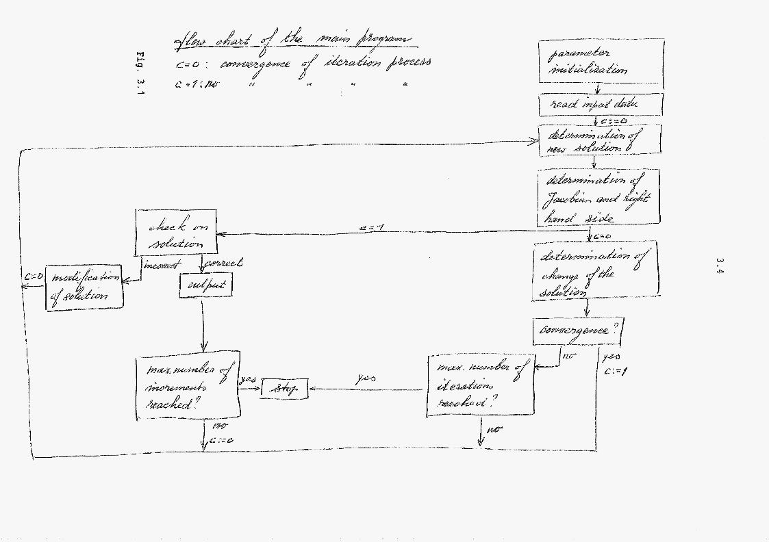
The standard routines can be applied to any problem, whereas the problem routines have to be supplied by the user. The present version o f t h e program contains 60 standard routines and l i problem routines. The way in which these problem dependent routines should be filled in will not be discussed here. The program itself includes a large amount of comments~ whereas for the problem-routines there is a description in the shape of a dummy-routine. This routine contains an explanation of a13 kinds of variables which have been used in the program. For the sake of clearness these variables have been named the same as much as possible as they have been defined in chapter 2. Wherever possible the program has been written in standard Fortran IV, so that the dependence on a certain type o f computer is made smaller t o the utmost. Taking into account the documentation at hand, here it will be enough for us to give a flow diagram of the main program. In the following section this will be discussed.

3.2

3 .2 Explanatory remarks on the main proqram

A block diagram of the main program is to be seen in Figure 3 . 1 . The way in which the program is carried out is shown in it by the direction of the ar- rows and depends on the parameter c according to its definition with Figure 3.1 . We shall now discuss some blocks of this scheme briefly.

* The block “input-reading“ . In this block the input is read from a diskfile. A number of standard parameters are read, such as an initial estimation f o r the position and orientation o f the bodies, the number of line ele- ments and the co-ordinates of the insertion points belonging to them, the maximum number o f iterations and increments. In addition the user may read quantities yet wanted through a routine gaven by himselflherself.

In this context by the new-solution is meant the sum total o f the last obtained solution indicated by xk-’ plus the change of the solution.

* The block “new-solution determination“.

k indicated by iq. Therefore the new solution, 3 I follows from

By the solution i s meant the solution o f the set of equations foa-mulated in section 2.8 . This block includes a routine which should be supplied by the user, viz. a routine with which from the column A l the new rotation matrix can be calculated. A s outlined in appendix 1 3 , namely with the help of this column the change of the rotation parameters can be calculated, after which with the new rotation parameters the new rotation matrix has to be calculated. In a number o f cases the column Ax equals (3, namely when

the parameter C has the value O.

* The block “determinatian of Jacobian and right hand side”. In this block the Jacobian and the right-hand side as given in relation (2.160) are determined. This block includes a number of routines which have to be supplied by the user, viz. - a routine for the calculation of the geometrical quantities needed in a contact point with the help of given surface parameters y or y.

- a routine for the calculation of the quantities which are connected with the kinematic conditions.

3 . 3

- a routine for the calculation of the quantities which are connected with

- a routine in which for the line elements in case of given lengths of the the external load.

elements, the force in and the rigidity of the elerrient are calculated.

* The block "convergence?" This black includes the examination whether the obtained solution satisfies a Convergence criterion of the following form

Ax is here the modification of the solution as determined with the help of

the Jacobian and the right hand side; qk-' is here the solution which ex-

ists at that moment. this convergence criterion i s only one out of the large number of convergence criteria. Modification of it may take place rather easily.

* The block "Solution-checking" . When after convergence the solution 5 at the end of an increment has been

determined, in this block the check will be made whether the contact-force is positive in all contact points. The contact-points for which this is not the case are then eliminated whereupon the calculation for the increment in question will be made again. So far the essential parts of the main program. A further explanation does not seem very relevant because this explanation can hardly be Given without. ent-ering into details. As said already in section 3 . 1 , for poten- tial users there is sufficient documentation for the application af the program.

3 . 4,

Fig. 3

.2

Chapter 4

Some examples

In this chapter the solutions -both numerical and analytical- of three rela- tively simple small problems are given. These problems include as rigid bodies a sphere and a cylinder where the sphere can move within the cylinder. For the sake of simplicity we have arranged for the movement to be two-dimensional. In the nature of things the program analyses these problems three-dimensionally. If no mention is made of it t h e variations of the two- dimensional movement as a result o f inaccuracies in the numerical solution process, may be suppose6 zero. These small problems give an opportunity t o demonstrate and test a large number of possibilities of the programs whereas at the same tiate an impression can be given of the calculation time needed. This calculation time, however, will strongly depend GE the type of the cai- culator used.

4.1 Description of the seometries of the sphere and the cylinder

The cylinder is supposed to be fixed in space (Fig. 4.13. The surface parameters we choose for a point on the inner wall of the cylinder are the polar co-ordinates tp and z. The position of a point on the inner wall is then given by

( 4 . 2 ) -9 -+ c = a cos tp 2, i- a sin cp 2 + z e, Y

Applying the derived theory of chapter 2 , the normal can then be written as follows :

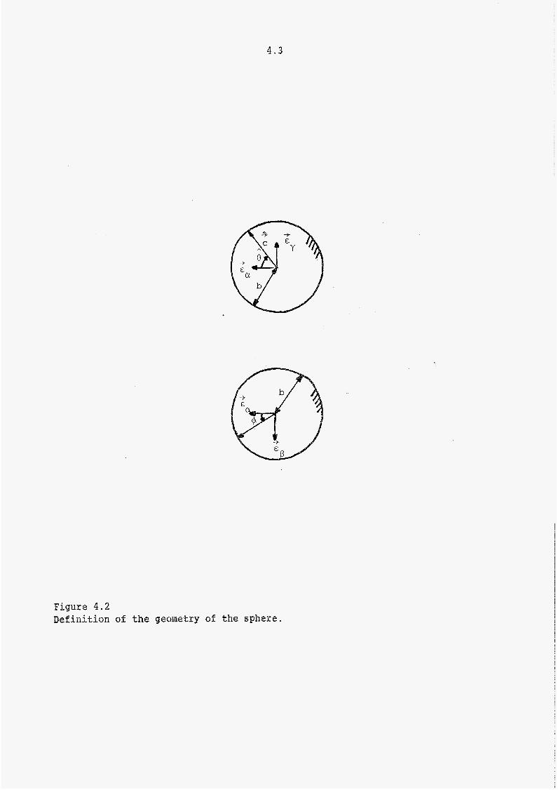
( 4 . 2 ) t -t n = cos tp e, + sin tp ey Far the geometrical description of the sphere the surface parameters we choose are the spherical co-ordinates tp and O . For a point on the outer wall. of the sphere it then holds that (Figure 4 . 2 )

s t c = b cos I$ cos Êl YO i- I3 sin I$ cos B Ego i- b sin 8 2 (4.3)

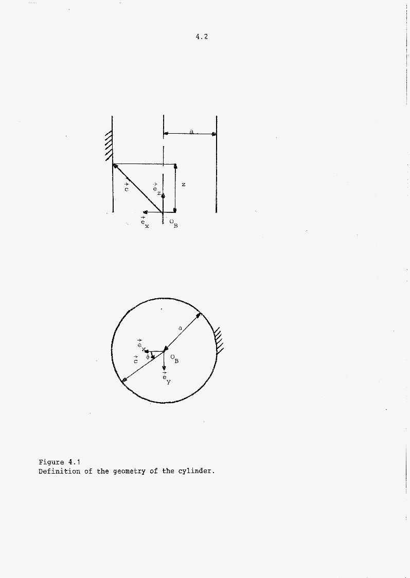
4.2

-+ e I oB X

Figure 4.1 Definition of the geometry of the cylinder.

4.3

Figure 4.2 Definition of the geometry o f the sphere.

4.4

* -P Here the directions of the base vectors E,, and eYO, respectively, are -* -P equal to the directions of the base vectors d,, e

starting position it should hold that R=I. Provided that cos O f O €or the normal we have:

en eZ, because in the Y

When cos û = O, the tangential vectors are dependent, which we excluded in principle. This dependence is always checked in the program, and if neces- sary a mistake being made is made mention of. Therefore, in principle we must exclude the points having cos 8 = O. However, we can choose the move- ments in such a way that these points cannot be a contact point, in conse- quence o f which we need not pay any further attention to this fact.

4 . 2 Description of the rotations

In the examples t o be dealt with we shall describe the occurring rotations with the help of the Cardan angles, which were discussed in appendix B. We shall choose the movements In such a way that only in the x-z plans rota- tions will occur. As a result we can write the rotation tensor introduced in appendix D as follows:

in which w the rotation is which % i t h the help oi the corkscrew rule is coupled to the positive y-axis.

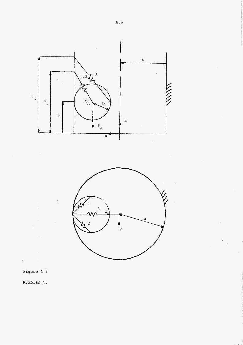
4.3 Problem 1

In this problem (Figure 4.3) we assume the sphere to be in point-contact with the cylinder. The sphere is connected to ground by means of 3 identicctl line elements. The external load is a force acting in negative z-direction ff,). Should the translation be prescribed in z-direction the remaining un- knowns are : - the position o f the contact point - the angle of rotation w - the contact force p in the contact point

4.5

- the indeterminate multiplier o which is connected with the load needed for the prescription o f the translation in z-direction.

Together with the theory given in chapter 2, these quantities can be deter- mined analytically, assuming that the movement takes place in the x-z plane, which on account o f symmetry will be the case. We shall not give this derivation in detail here but discuss the main points of it. On account o f syinmetry, for the contact point on the cylinder wall it will hold that QP-O and ditto rp=O for the contact point on the spherical wall. The position o f the contact points on the bodies is then determined by h (Figure 4.3) and 8. A f t e r some calculations this information together with a prescribed translation $ in positive z-direction yield from the contact con- ditions (2.47) and (2.48).

h = $ ( 4 . 6 1

9 - w 1 4 . 3 )

The load on the body can be determined as follows: the external load is given by :

t 2 e = -fe e,

ge = 8

whereas the load resulting from the point contact is given by:

3 - - p a . 3 n = - P e x * k -

(4.8)

( 4 . 9 )

(4.10)

As t h e translation in z-oirection is prescribed, in this case the kinematic condition is as follows:

( 4 . 1 2 )

This has the consequence that the load as a result o f these conditions is given by (relations (2.611, (2.212) and (2.113)):

?fr = -0 gz (4.13)

4 . 6

s S

I

1 S

e

I I

Z

Figure 4.3

Problem 1 .

4 . 7

itr = 8 ( 4 . 1 4 )

For the line-elements, as a constitutive connection we take:

2 f(L) = A . L + E . L ( 4 . 1 5 )

With the help of the insertion points as given in Figure 4 . 3 and the theory from section 2 . 6 it can be derived that the total load in consequence o f the elements is given by:

L: = 2b2 +- ( @ - si ) 2

it

Y ml = - I A + B E3)(b COC w ( @ - s3) - b2 sin w ) g

( 4 . 1 6 )

(4 .17 )

( 4 . 1 8 )

( 4 . 1 9 1

With the help o f the equilibrium of forces and moments and the given expres- sions for the loads, it then follows that the following must hold:

tan w = f P - s 3 m (4.20)

(4.21)

( 4 . 2 2 )

Together with h=@, 8=w and given value of F: herewith the solution is known. This problem has also been analysed with the help of the program. For this analysis the following numerical values have been chosen: a= 2 cm, b = 1 cm, A = 1 N/cm, B = 2 N/cm sl = 5 cmf s3 = 6 cm, f, = 50 A .

In the figures (4 .41 , ( 4 . 5 ) and ( 4 . 6 ) for a number of quantities the exact solution is shown by means of full lines: the solution calculated for a num- ber o€ given values of 8 is shown by means of dots. The deviations found are

2

4 . 8

w igrl

z

-2-1-9-

1 0 -1 - t o [ c n l l 4 3 2

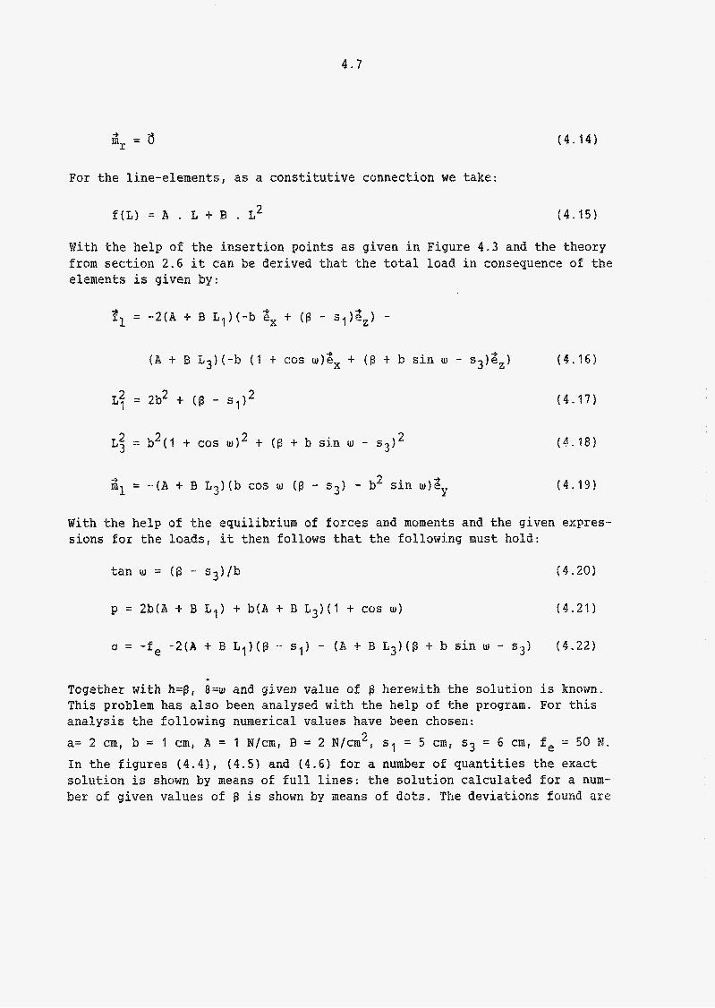
Figure 4.4 Angles of rotation as a function of the prescribed translations.

4 . 5

L Lcm

t I

7

6

5

4

3

2

1

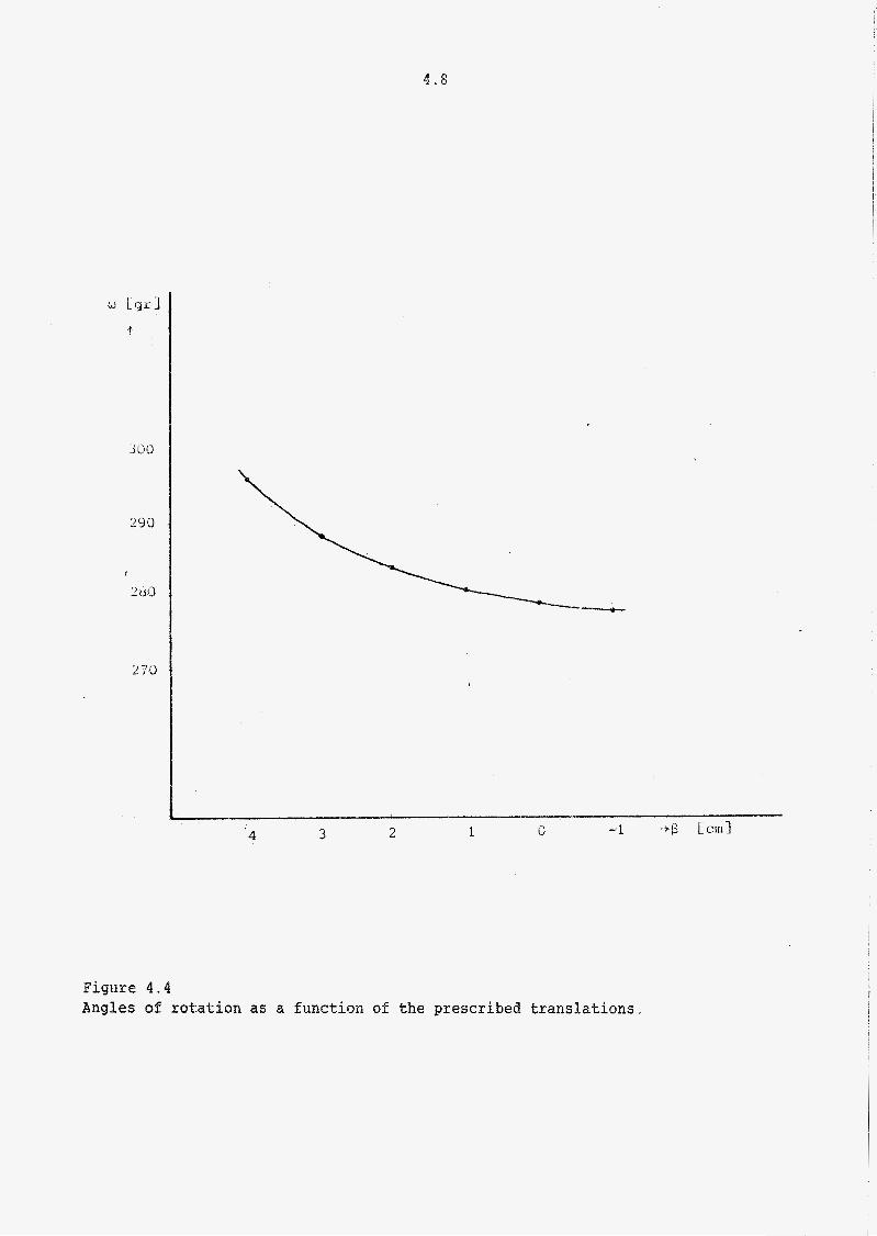
Figure 4.5 Lengths sf the elements as a function of the prescribed translations.

4.10

i.? [ N

t

L ï t

..Li!

5c

50

LO

10

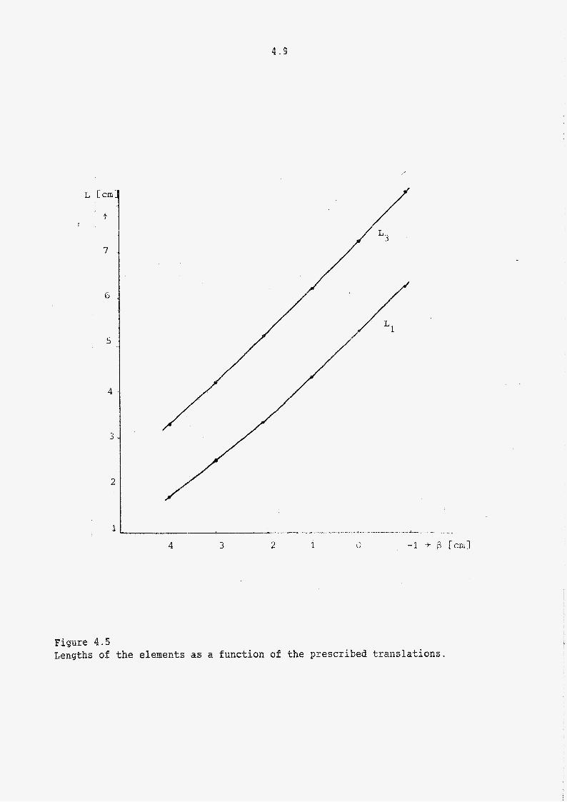
Figure 4.6 Fctrces as a function of the prescribed translations.

4 . 4 1

minimal which, of course, is also determined by the parameter E in the con- vergence criterion as mentioned in section 3.2. In these calculations this parameter has been puf. at 0.01.

The total amount of calculation-time for calculating 6 positions of equi- librium was 17 sec. (Prime P550) with 4 iterations needed per increment.

4.4 Problem 2

In this case no point o f contact occurs (Figure 4.7). The sphere is con- nected to ground by means of 6 line-elements of which the dements 1, 2 , 3, 5 and 6 are identical. Owing to symmetry, only in the x-z plane movement will OCCUK. If we prescribe the translation in x and z directions now, we shall have the foll~~ing unknowns: - the rotation w - the indeterminate multipliers We can determine these quantities with the help of the equilibrium equations. The occurring loads are given by:

and 0 2 .

ze = -f -? e

me = 8

mr = 8

because in this case the kinematic conditions are:

k , = e , . a - a = o -?

( 4 . 2 3 )

( 4 . 2 4 )

( 4 . 2 5 )

( 4 . 2 6 )

( 4 . 2 7 )

( 4 . 2 8 )

1 S

a

Figure 4 . 7 Problem 2 .

4. '13

Figure 4.8

Indeterminate multipliers as a function of the translation.

4.14

The load as a result of the line elements can be determined from the inser- tion points o f the eleinents as given in Figure 4.7 and the constitutive relation for the elements:

f(Lf = L element 1, 2 , 3, 5 , 6

f(L) = L - Lo element 4

(4.29)

(4.30)

From the equilibrium of forces and moments it then follows that:

( 4 . 3 2 ) 2 2 2 L3 = (ct - a “r b cos u a I 2 -+ b sin w

o2 = -fe - (Lo b sin w)/L3 (4.33)

s i n w = O (4.34)

Far the sake of the stability o f equilibrium it musk hold that w-0, which gives :

“1 = -Lo - 4a ( 4 . 3 5 )

o2 = -fe ( 4 . 3 6 )

With the numerical values f,= 4 N, s1 = 6 cm, h = 3 cmr Lo = 1 cm, a = 2 cm, b = 1 cm, and a number of values for the translation a in x-direction, with the help of the program the corresponding posieions o f equilibrium have been determined. The calcu- lated and exact values f o r o1 and u2 are almost the sane and are given in Figure 4 . 3 . The total amornlt of ~â~culation-time for this problem ( 4 gosi- tions o f equilibrium) was 12 sec., with 2 iterations required per increment.

4.5 Problem 3

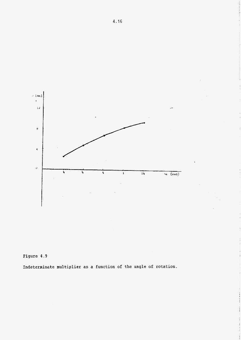
In this example the configuration is equal to the one of problem 2 (Figure 4.7). All elements are now taken identically with f(L)=L, so that the con- figuration becomes omnilaterally symmetrical. We now prescribe the rotation w . AL; a result this condition should be written as:

4.15

K = w - w g = 0

and yields as a load a moment

-+ ii

Y mr = -CT e

( 4 . 3 7 )

(4.38)

which can be proved with the relation (2.611, (2.1121# (2.113) and the ïela- tions for 6 w in appendix D. With the help of force and moment equilibrium it can be derived that:

6 = (S., 9 4h - €,)I6 = translation in z-direction

a = 0

IJ = -b ( sq + 2a)sin w

= translation in x-direction

(4.39)

(4.40)

14.41)

As a result, on account of general symmetry the sphere remains on the symmetry-line o f the cylinder, which can be expected, as well. With t h e numerical values as given in section 4.4 we have the following:

i @ = 23

cr =-IO sin w

(4.42)

(4.43)

In Figure 4.9 the calculated and exact value of cr fox a number of values of w is shown, whereas tihe calculated value of 13 was exactly in agreement with the exact value. The calculation-time needed for 5 increments was 12 sec. with 3 iterations required per increment.

4.6 Remainins oss si bi li ties o f the Prouram

The exanples presented in the foregoing may have given an impression of a number o f the possibilities offered by the model and the program. One pos- sibility has not been discussed, viz. the simulation of cancellation of a contact point. Of course this has been tested indeed, and that with the help o f the problem as formulated in section 4.3. For this purpose in a certain position o f equilibrium such an external load has been applied that - theoretically- the contact point must cancel (force in negative x- direction). This was then calculated nicely by the program. At the same time

4.16

Figure 4.9

Indeterminate multiplier as a function of the angle of rotation.

4.17

we see here another possibility of the program viz. to take into account an external load which is dependent on the position and orientation of the moving body. Consequently, vanishing of a contact point can be simulated, whereas this does not hold good for the appearance of a new contact point because here no numerical determination is possible. This should be done by other means. In case o f the determination o f a new contact point being in existence (for example in a graphical way), this contact point can be intro- duced as yet with the help of the restart option, which is a part o f the program.

Chapter 5

Application and extension of the model

Introduction

As mentioned in the introduction of this report, the model described here is a generalization of the model of the knee developed by Wismans [ 3 ] . This generalization offers a number of possibilities for the use o f the model in the future. A number of possible extensions can be made t o it, as well. On the following pages we shall enter into one thing and another.

5 .1 Comparison with the Wismans'model

The model described in this report contains a number of extensions with respect t o the Wismans'model. These are: - the theoretical substructure is based on a co-ordinate-free notation which in principle makes it possible t o describe the movements with respect to a v e e b r base chosen at will.

- the geometry of the contact surfaces may be chosen relatively arbitrarily, whereas the numerical description of the contact surfaces can also be chosen freely .

of equilibrium.

the moving body.

- the number of contact points and kinematic condition may vary per positon

- the external loa6 may be a function of the position and the orientation of

~ n ~ t h e ~ difference with the ~~ismans'model is the fact that the calculation time needed, probably is essentially shorter. This supposition is based on the calculation time which was needed f o r the small problems presented in chapter 4 , and the knowledge that the calculation time for the Wismans'model has to be expressed in OUTS. The extensions mentioned will permit working a model of the knee containing more possibilities than the Wismans'model. The quality of this model of the knee, of course, indeed depends on the degree to which assumptions have been made to come t o a model of the knee which can be described wit.h the theory set out in this report. Furthermore, the numerical elaboration will be influenced strongly by the quality o f the description of the relevant quantities like geometry, line elements and load.

5.2

5.2 Extensions of the model

In the model a number of essential assumptions have been made with respect to the properties of the contact surfaces. It has been assumed that these surfaces are infinitely rigid and that only point-contact occurs. In many technical and biomechanical constructions these requirements will not have been come up to. The contact surfaces may deform (strongly) and the point of contact may degenerate into line or two-dimensional contact. T h i s degeneration o f the point-contact cannot be described with the present model. Perhaps the model could be adapted that way. For this purpose both the theory and the software should then be changed. In this context the admittance of line contact may be thought of, e.g. the contact force results from a distributed load which can be described with an u ~ k ~ ~ o w n parameter. (e.g. evenly distributed load). The admittance of a deformable surface involves many bigger problems. In that case a combination of continuum and rigid body mechanics will have to be found for the description of the problem. It. needs no explaining that ~ u c h a combination could produce a much mare extended model which, however, in proportion is also more complicated. Should, however, the deformations of the contact surfaces be small with respect to the occurring rigid movements of the body, the results of this model could possibly be used afterwards for an analysis of the deformations of the contact surfaces. This analysis can then be made retrospectively because in the first instance these deformations can be left out of consideration.

In this report a model has been described for the determination of positions of equilibrium of two coupled rigid bodies. The methodology applied, however, also seems suitable €or the development o f a model in which several rigid bodies are in contact. A large nmmber of elements of the model will a lso play a part if the determination is considered of positions af equilibrium of several coupled rigid bodies. The descriptive set of equations and the resolution of them -dependent on the couplings made- will be more complex but have the same structure. The development of such a model would, however, indeed require an ent.ire new theoretical substructure and numerical elaboration.

On the basis o f these considerations it seems that follow-up stuibies o f this subject can be made very well. These studies could make the model suitable for a wide range of practical problems.

Apuendix A

an an Determination o€ expressions for and

We start from relation ( 2 . 2 4 ) .

t n = sn cu -+ * CV/icu -* * t cVI

From this it follows that:

Premultiplying relations (A2) now by Ï! and considering that relation ( A l ) gives :

n . CC, * E,, = SnlZu * $,I

-* whereas from $ . n = 1 we have:

n . = = o an"

for relation (A2) it then follows that:

Substitution of relation ( A 5 ) in relation (AS) yields with the help of the identity :

(5 ?t - I) . "v = d * (% * 4) for each "v

A. 2

Substitution of the relations:

a?, + -4 f3% 3 * (Cv * au) = cv n . au

-4 s, cv * n!IZu * C,I = If,

as In a quite analogous way for the vector E it follows:

= = - ( 3 - K an %)p a%)$ v

Appendix B

Determination of 6; and ü? in case of 6; and 68 being given.

We start from the relations ( 2 . 5 2 ) and (2.53), mentioned here in a shortened version as follows:

(K + R . i . Rc) . 65 = i!,

( K + R . i . Rc) . R .

First o€ all we notice that the tensor K 9 R . K . Rc is singular because: -? ( K + R . I S . R ~ ) . n = 6

This is a direct consequence of the definitions of the tensors K en K and of the fact that relation (2.48) has to be satisfied. Furthermore, it holds that this tensor is symmetric because the tensors K and K are symmetric. This means that this tensor contains 3 real eigenvalues and eigenvectors. The eigenvalues are indicated by u,, u2 and u3 and the corresponding

eigenvectors by ml' a2 and G3. The amounts of the eigenvalues are chosen in such a way that it holds that:

u3 = o

4 -B a m 3 = n = - R . n

+ - 4 m. mi = i (summation conventian applies) 1

Using the spectral representation of a symmetrical second-order-tensor, it then holds that:

Now we shall define the pseuda-inverse P of the tensor K t R . K e Rc:

B.2

for which it then holds:

P . (K t A . . Rc) = $1 m l i- $2 8,

For the relations ( B I ) and (B2) we then have:

($, w , t Ïi2 8,) . oc = P . f1

(&, E, t Ïi2 w21 . R . id = P . ip,

2 . 6 2 = i ; t 3 * o b = o

d . R C . R . ü i ? = - m 3 . R . & = O

With relations ( 2 . 2 2 ) and ( 2 . 2 4 ) it now gives:

4

so that we can write relations (B lo ) and ( B I I ) as follows:

- 4 4 mi mi . 82 = iG = P . f 1

m i m i . R - d = ~ . B ~ = P . P, + + 4

(€3141

The variations 62 and 68, therefore, can be d e t ~ ~ ~ i n e d from:

6 c " = P . (BI61

68 = RC . P . f2 (BI71

With this, with relations ( 2 . 2 2 ) and (2.26), consequently it follows that:

ou = 8, . tic = gu . P . t , (BI 8 1

Bv = i fv . aC = iJv . P . t ,

Analogue relations apply to Bil and 69.

Appendix C

Variations in loads as a result o f point-contact

We take the relations (2.101) and (2.102) as starting points:

From relation (2.38) it follows that:

i 3 brik = -Kk . 6Ck

whereas in appendix $ the following derivation has been made:

% i oCk = RC Pk . * (R . i k ) - Kk * f 6 3 * (R . C k ) I f

Now we shall define the following skew-sy~e~ric tensors:

fC3)

%k . ;i = (R ($k * ik)) * $ (C7 1

Substitution of relations ( C 3 ) up to and including (C6) in relation ( C l ) then yields:

with :

c.2

S u b s t i t u t i o n of r e l a t i o n s (C3) up t o and i n c l u d i n g ( C y ) i n r e l a t i o n ( ~ 2 1 g i v e s :

w i t h :

D . 2 Y

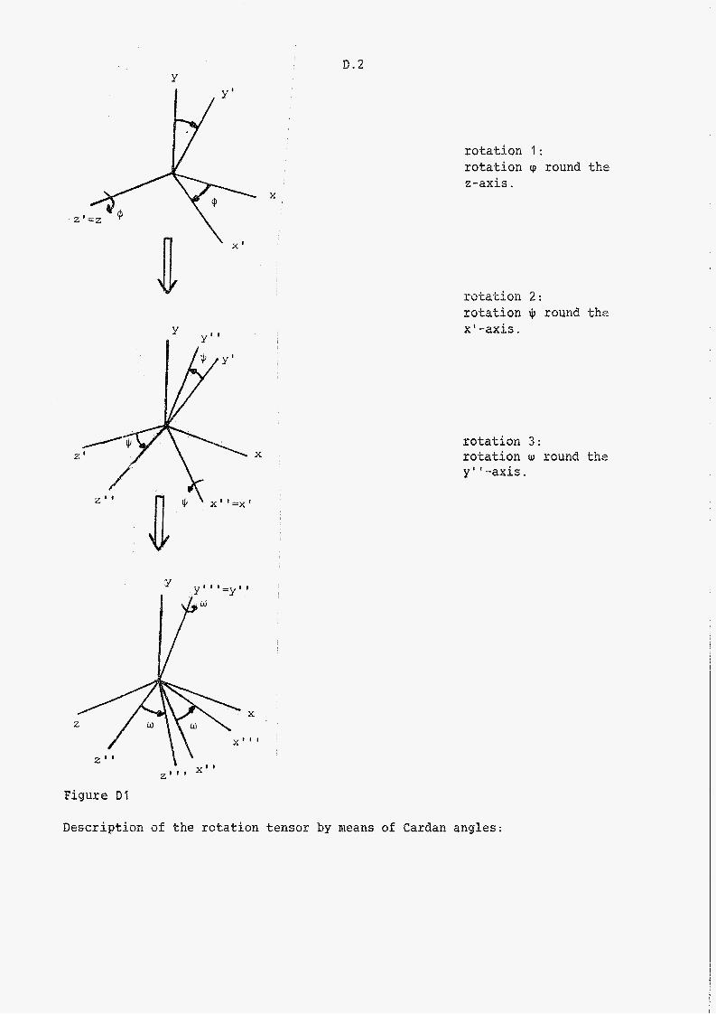
X

rotation 1 : rotation rg round the z-axis.

rctation 2: rotation $ round the x' -axis.

rotation 3 : roÉation w round the y' I -axis.

Figure Dl

Description o f the rotation tensor by means of Cardan angles:

0.3

-? i- (6 ip t sin 41 6w)e, (03)

W i t 3 this relation we can express the variations 69, sit and 6 w in the vector 88. It appears t o hold:

1 i+ i+ 6 w = (sin cp ex i- cos ip e 1 . 6 8 Y

These relations only apply if cos $ # O . If t j = O, we cannot calculate the variations 6vp, 6 $ and 6 w from the vector a t . In this case we can call this a kinematic singularity. Suppose we want ‘co prescribe the angle of rotation w by means o f a kimiematic condition. Here for the relation ( 2 . 5 9 ) it then holds that:

in which wo is the desired value o f w . In this case for the relation (2 .61 )

it then applies:

Therefore, with relation (D5) the following holds:

1 i+ i+ 6 w = (sin ip ex i cos u, e,) . 6 8 = O

For the vectors 2 and 3 introduced in relation (2.61) it then holds that:

if=---- ’ (sin ip zX + cos u, cos tj.I

From the relation (D10) and (DI11 I for the tensors DI, D2‘ D3 and D4 introduced in relation (2.116) and ( 2 . 1 1 7 ) < the following applies:

B.4

consequently:

Dl = o

D2 = O (DI31

D3 = O

+ - P D4 = + (8, e, - e, e,) cos Q

Another example o f a kinematic condition can be that a component o f the translation vector 2 is fixed, e.g. the z-component. I% then follows that:

-B a k = e , . a - a o

It i s a simple matter to determine that i n this case it holds that:

+ - P Ex = ez (DI81

E. 1

External load on the body A

Two examples of an external load on body A are discussed here, viz. a force with a constant magnitude and space-fixed direction and a force with a constant magnitude and direction with respect to the body A (a follower force). In the first example we shall consider an external force being composed as follows z

(El j .d -9 3, = a e, + b ey + c e, (arbic are constants)

Consequently this force has a constant magnitude and direction with respect to an inertial frame. As 65, = 6, €or the tensors Fe and Fe given in the relation (2.1071, in this case therefore it holds that:

1 2

FA = Fe = O

In the second example we shall consider an external force on the body A which acts as a follower force, that is:

With the help of the rotation tensor R we can also write this relation as:

For the variations 63, it then holds:

that is :

tee = 6% * 1,

Mow we shall introduce a skew-symmetric tensor Fe with:

E.2

F, . w" = P, * w' for ail W

For relation (E61 then, the following applies:

1 2 In this case the tensors Fe and Fe as given in relation (2.107) can now be written as:

Fe = O (E91

Fa = FE (E109

F. 1

Appendix F

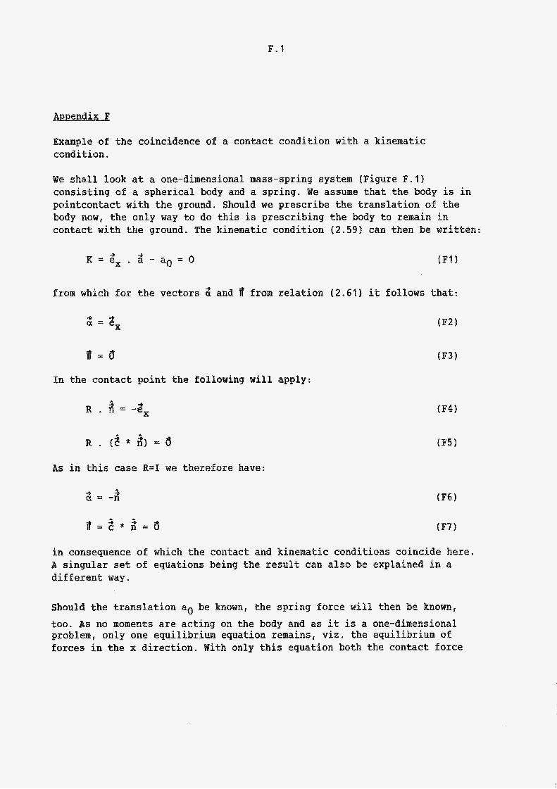
Example of the coincidence of a contact condition with a kinematic condition.

We shall look at a one-dimensional mass-spring system (Figure F.1) consisting of a spherical body and a spring. We assume that the body is in pointcontact with the ground. Should we prescribe the translation of the body now, the only way to do this is prescribing the body to remain in contact with the ground. The kinematic condition (2.59) can then be written:

* -B K = e x . a - a o = O

from which for the vectors 2 and $ from relation (2 .61 ) it follows that:

4 + a = e,

a = d

In the contact point the following will apply:

a 4 R . n = -e,

A s in this case R=I we therefore have:

4 1 a = -n

íF41

íF6ì

in consequence of which the contact and kinematic conditions coincide here. A singular set of equations being the result can also be explained in a different way.

Should the translation a. be known, the spring force will then be known, too. As no moments are acting on the body and as it is a one-dimensional problem, only one equilibrium equation remains, viz. the equilibrium of forces in the x direction. With only this equation both the contact force

and the force needed for the description of the kinematic condition have to be determined, which is impossible.

-i e Y

Figure F. 1

Mass spring system with point contact.