Embed Size (px)
Citation preview
symmetryS S
Article
A Model for Shovel Capital Cost Estimation, Using aHybrid Model of Multivariate Regression andNeural Networks
Abdolreza Yazdani-Chamzini 1 ID , Edmundas Kazimieras Zavadskas 2,3 ID ,Jurgita Antucheviciene 2,* ID and Romualdas Bausys 4
1 Young Researchers and Elite Club, South Tehran Branch, Islamic Azad University, 14115/344 Tehran, Iran;[email protected]
2 Department of Construction Management and Real Estate, Vilnius Gediminas Technical University,Sauletekio al. 11, 10223 Vilnius, Lithuania; [email protected]
3 Institute of Sustainable Construction, Vilnius Gediminas Technical University, Sauletekio al. 11,10223 Vilnius, Lithuania
4 Department of Graphical Systems, Vilnius Gediminas Technical University, Sauletekio al. 11, 10223 Vilnius,Lithuania; [email protected]
* Correspondence: [email protected]; Tel.: +370-5-274-5232
Received: 27 October 2017; Accepted: 29 November 2017; Published: 1 December 2017
Abstract: Cost estimation is an essential issue in feasibility studies in civil engineering. Many differentmethods can be applied to modelling costs. These methods can be divided into several main groups:(1) artificial intelligence, (2) statistical methods, and (3) analytical methods. In this paper, themultivariate regression (MVR) method, which is one of the most popular linear models, and theartificial neural network (ANN) method, which is widely applied to solving different predictionproblems with a high degree of accuracy, have been combined to provide a cost estimate modelfor a shovel machine. This hybrid methodology is proposed, taking the advantages of MVR andANN models in linear and nonlinear modelling, respectively. In the proposed model, the uniqueadvantages of the MVR model in linear modelling are used first to recognize the existing linearstructure in data, and, then, the ANN for determining nonlinear patterns in preprocessed datais applied. The results with three indices indicate that the proposed model is efficient and capable ofincreasing the prediction accuracy.
Keywords: cost estimation; shovel machine; neural network; multivariate regression; hybrid model
1. Introduction
Earthmoving and loading/unloading works are essential parts of construction processes.They require the use of heavy equipment. In spite of the fact that energy use and emissions arecritical when selecting the equipment [1], the cost is usually a crucial factor in the industry. In mining,loading is one of the most important operations, influencing mine preparation, design, and production.This activity has a significant share of the capital and operational expenditures. In the process of mineplanning, the loading system mainly determines what other pieces of equipment and what mode ofoperation will be used, and it is a key to low-cost production [2]. A shovel machine, which is a tool fordigging, lifting, and moving bulk materials, is the most common piece of equipment that is used toload rock material in surface mines. A shovel is a machine capable of handling hard, dense, abrasive,as well as highly fragmented ground, which can accurately spot for loading into dump trucks, railcars, loading hoppers, etc. [2]. Shovels are usually grouped into four classes [3]:
Symmetry 2017, 9, 298; doi:10.3390/sym9120298 www.mdpi.com/journal/symmetry
Symmetry 2017, 9, 298 2 of 14
• small shovels (0.5–2 m3 bucket size);• medium shovels (2–5 m3 bucket size);• large-size shovels (5–25 m3 bucket size);• very large-size shovels (with a bucket larger than 25 m3).
The selection of the best shovel among a pool of the existing alternatives based on the consideredcriteria can be performed applying the feasibility studies, which should be conducted to analyse theinvolved different technical, economic, and operational aspects. The most frequent technologicalparameters of shovels operations are analysed in the literature. As an example that is related tomathematical simulation a study presenting automated designing of swing circuit for a hydraulicshovel [4] can be mentioned. The effectiveness of mining equipment, namely trucks and shovel,regarding its useful employment without time losses were analysed [5]. For the considered equipmentselection problem, the mentioned numerous aspects of different nature can be effectively investigatedby using a multiple criteria decision making (MCDM) tool. MCDM methodology allows for combiningseveral important issues (criteria), also estimate the relative importance of the analysed criteria, as wellas to compare potential alternative equipment and to select the best suited in the analysed situation [6].
Besides equipment selection that is based on technical requirements, the production rate andcost-benefit analysis make the main parts of the feasibility studies. Cost estimation with variouspurposes takes a significant place at different stages and processes in mining and related industries.During the planning stage, machine specifications, like technical and operating features, and,accordingly, the costs are not available in in the mineral fields, unlike other areas [7,8]. Therefore,developing an up-to-date model with sufficient accuracy is essential. There is a number of modelsfor estimating mineral industry costs, such as the cost estimation to small underground mines [9],the evaluation of mining equipment, as well as mineral processing equipment costs and other capitalexpenditures that are related to mining and processing operations [10,11], as well as cost estimation thatis adapted for the peculiarities of the Australian mining industry [12], the system of cost estimation inmining of metallic, as well as nonmetallic minerals in two countries, comprising Canada and the UnitedStates [13], a cost model for preliminary feasibility study and a different cost model for a detailedfeasibility study, including exponential regression and multivariable linear regression, implemented inIranian deposit of copper [14], a case study of South Africa for calculation of capital costs for setting upa coal mine [15], and Hard-rock LHD cost estimation [7]. A methodology of evaluation of ore bodiesand a guide for practical application was suggested [16–19].
An individual question of feasibility evaluations applying simplified cost models wasanalysed [20]. A guide for the mining sector, including mining and energy valuation, and beingfocused on Australian investors and managers [21], was prepared. Also, energy costs of equipment asa significant part of costs in mining activity were evaluated, including not only processing costs butalso transportation and exploitation costs of machinery [22].
The models mentioned above often take into account only one parameter as an independentvariable, while the constructed models are merely based on the regression analysis. Therefore, it isessential to develop a more accurate and efficient model for cost estimation of equipment.
The different techniques can be applied for the optimization problems. During the last decade,significant research has been performed on fuzzy logic control of the nonlinear systems [23,24].Another direction of the optimization techniques is artificial neural networks.
The Artificial Neural Network (ANN), which is one of the artificial intelligence methods, as wellas multivariate regression (as one of the statistical models), are powerful tools for pattern recognitionand modelling. These two methods are used by various researchers.
An ANN-based model for estimating distillation process, using the Levenberg–Marquardtapproach is developed by Singh et al. [25]. Yamamura [26] predicted pharmacokinetic parameters by anANN modelling. An ANN prediction model for determining the failure depth of coal seam floors wasdeveloped by Lian-guo et al. [27]. They compared calculation results with the real case study and statedthat the predicted results by applying the suggested model agreed well with practical measurements.
Symmetry 2017, 9, 298 3 of 14
An ANN model for an industrial gas turbine was developed by Fast et al. [28]. They used theoperational data with a multilayer feed-forward network to construct an ANN model. Analysing theresults, they made a conclusion that some of the functional and performance parameters of the gasturbine, including a critical parameter of identification of the anti-icing mode, can be accuratelypredicted in a changing modelling environment. Lee et al. [29] suggested a way to improve thereliability of the Bridge Management System, using the ANN-based Backwards Prediction Model.
Jalali-Heravi et al. [30] developed the shuffling multivariate adaptive regression splines andthe adaptive neuro-fuzzy inference system as tools for studying a quantitative structure-activityrelationship (QSAR) of severe acute respiratory syndrome (SARS) inhibitors.
Verlinden et al. [31] presented a case study and estimated the cost of sheet metal parts, usinga combination of multiple regression and artificial neural networks. Mesroghli et al. [32] used theregression and artificial neural networks for estimating gross calorific value based on coal analysis.Sahoo et al. [33] developed the models for predicting stream water temperature, using three techniques,namely the regression analysis, an artificial neural network, and also combining them with chaoticnon-linear dynamic models. Therefore, it is clear that the ANN and regression have demonstratedtheir capabilities of modelling engineering practice problems.
An application of neural networks for improving the weighting precision, having the aim tooptimise loading of trucks, as well as production efficiency of electric shovels, was presented byGu et al. [34]. The combination with fuzzy logic was suggested to decrease uncertainties in the process.
During the recent years, the different aspects of civil engineering problems have been consideredwhen applying artificial neural networks (ANNs). Suspended-dome model updating was performedby back propagation network approach to evaluate the discrepancy between actual structure and thecorresponding numerical approximation [35]. The ANN approach was applied for the estimation of theaxial bearing capacity of the rectangular concrete-filled tubular columns [36]. A stochastic conceptualcost evaluation of the highway projects is performed by generating an empirical distribution ofthe estimated cost range, without additional initial assumptions [37]. This empirical distribution isconstructed applying ANN techniques and bootstrap sampling. The application of ANN techniqueswas implemented to study construction labour productivity [38]. Additionally, the different ANNactivation and transfer functions are applied to estimate the most influencing factors to modelconstruction labour productivity. The parameter sensitivity analysis for civil engineering problems wasperformed implementing ANN algorithms [39]. This paper dealt with parameter sensitivity analysisparadigm, in which the essential element is neural network ensemble.
Usually, structural health monitoring of the engineering systems is governed by fixed orhand-crafted features, and this fact significantly reduces the reliability of such monitoring systems.The proposed structural damage detection system, which was constructed by implementingone-dimensional (1D) convolutional neural networks, allows for extracting damage-sensitive featuresfrom raw acceleration information [40].
The prediction problem of the capacity characteristics of the pile structures has been modelledimplementing ANN and principal component analysis [41]. The issue of the claim management inthe construction projects was solved applying neural network approach [42]. The proposed approachallows for not only classifying and ranking emerging claims, but also to predict the claim frequency inthe construction projects.
The integration of two different information flows: spatial planning of buildings and territorialplanning system, was performed while applying ANN technique [43]. The evaluation of the uncertaintyinfluence to the estimated cost of the construction projects was carried out implementing differentmodels for the training and evaluating phases [44]. For training phase, fuzzy adaptive learning controlnetwork and the fast, messy genetic algorithm were applied. For evaluating phase, component ratios,regression, and multi-factor evaluation sub-models are accomplished.
In this paper, multivariate regression and ANN models are employed to construct a hybrid modelto yield a more accurate and precise model than traditional multivariate regression and ANN models.
Symmetry 2017, 9, 298 4 of 14
In the proposed approach, a model is considered as a function of linear and nonlinear components,so that the multivariate regression model is first employed to recognise the existing linear patternin data. Then, the ANN is applied as a nonlinear function to model the preprocessed data. Finally, themain performance criteria of the model are calculated, including the coefficient of determination (R2),Normalized Mean Square Error (NMSE), and Mean Absolute Percentage Error (MAPE), and the bestmodel is identified according to calculation results.
2. A Multivariate Regression Model
The method of multivariate regression (MVR) is used to determine the relationships betweenindependent and dependent variables. It might also be used for analysing the data or generatinga model [45]. In statistical analysis, the mathematical form of an MVR model is determined by thefollowing equation:
Y = Xβ + ε (1)
where ε addresses the N × 1 vector of observations for the disturbance term, X represents the N × kmatrix of observations of the k-independent variables, β expresses the k× 1 vector of parameters, andY denotes the N × 1 vector of observations of the dependent variable.
The best prediction of Y (the variable Y regressed on X), based on basic assumptions of the linear
model, is denoted as_Y , and can be obtained by the following equation:
_Y = X(XTX)
−1XT , (2)
where Y is the shovel capital cost (CC), and X = (1, BC, BL, W, HP) is a set of independent variablesdefined, respectively, as a constant term, bucket capacity (BC), boom length (BL), weight (W), andhorsepower (HP). Thus, the model is expressed by
CC = b1 + b2BC + b3BL + b4W + b5HP + e, (3)
where b1 is a constant term; b2, b3, b4, and b5 are the regression coefficients; and, e is an error term.
3. An Artificial Neural Network
The ANN technique, a branch of artificial intelligence methods, is a reliable and usefultool for the formulation of linear and non-linear patterns. Bourquin et al. [46] revealed that anANN methodology shows a clear superiority as a modelling technique, in comparison to classicalmethods, for data sets showing non-linear relationships, and this is for both data fitting andprediction abilities. This technique is widely used for many scientific and engineering problems, such asdata processing, classification, and pattern recognition. The ANN technique has some unique features,distinguishing it from other data processing systems. This technique, even when partly damaged,can work successfully. This method can also be used for parallel processing, generalisation, anddemonstrates low vulnerability to errors in the dataset [47]. An ANN model employs the mechanismthat is applied in the human brain to extract the patterns and behaviours of data [48].
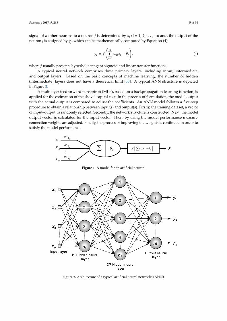
The ANN technique has been developed based on the structure of biological neural networks,where neurons are the backbone of the structure. The inspiration for an artificial neuron arises from abiological neuron; so that, an artificial neuron can send signals to other neurons. Then, it collects thesesignals, and when fired, it transmits a signal to all of the connected neurons [49]. Figure 1 graphicallyshows a typical artificial neuron.
From Figure 1, the transfer function is shown by f ; the activation threshold of the neuron j isdetermined by θj; the connection weight between the ith and jth neurons is assigned by wij; the input
Symmetry 2017, 9, 298 5 of 14
signal of n other neurons to a neuron j is determined by xi (I = 1, 2, . . . , n); and, the output of theneuron j is assigned by yj, which can be mathematically computed by Equation (4):
yi = f
(n
∑i=1
wijxi − θj
), (4)
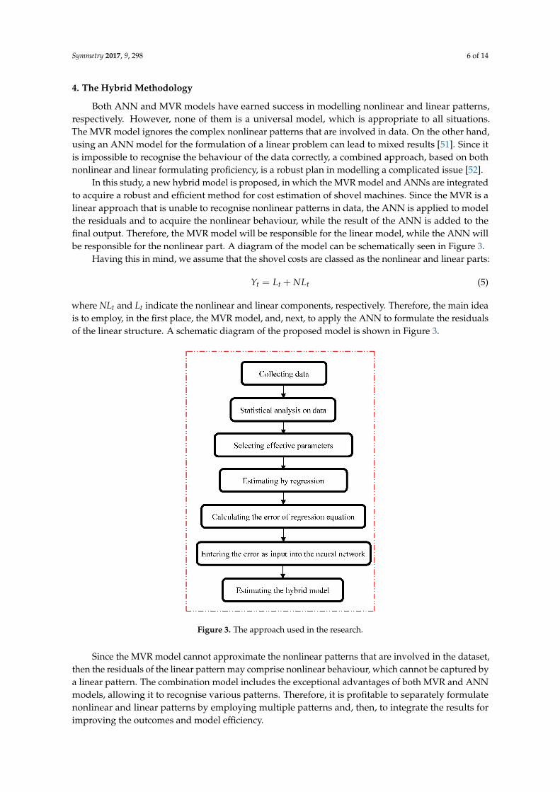
where f usually presents hyperbolic tangent sigmoid and linear transfer functions.A typical neural network comprises three primary layers, including input, intermediate,
and output layers. Based on the basic concepts of machine learning, the number of hidden(intermediate) layers does not have a theoretical limit [50]. A typical ANN structure is depictedin Figure 2.
A multilayer feedforward perceptron (MLP), based on a backpropagation learning function, isapplied for the estimation of the shovel capital cost. In the process of formulation, the model outputwith the actual output is compared to adjust the coefficients. An ANN model follows a five-stepprocedure to obtain a relationship between input(s) and output(s). Firstly, the training dataset, a vectorof input–output, is randomly selected. Secondly, the network structure is constructed. Next, the modeloutput vector is calculated for the input vector. Then, by using the model performance measure,connection weights are adjusted. Finally, the process of improving the weights is continued in order tosatisfy the model performance.
Symmetry 2017, 9, 298 5 of 13
A typical neural network comprises three primary layers, including input, intermediate, and output layers. Based on the basic concepts of machine learning, the number of hidden (intermediate) layers does not have a theoretical limit [50]. A typical ANN structure is depicted in Figure 2.
A multilayer feedforward perceptron (MLP), based on a backpropagation learning function, is applied for the estimation of the shovel capital cost. In the process of formulation, the model output with the actual output is compared to adjust the coefficients. An ANN model follows a five-step procedure to obtain a relationship between input(s) and output(s). Firstly, the training dataset, a vector of input–output, is randomly selected. Secondly, the network structure is constructed. Next, the model output vector is calculated for the input vector. Then, by using the model performance measure, connection weights are adjusted. Finally, the process of improving the weights is continued in order to satisfy the model performance.
Figure 1. A model for an artificial neuron.
Figure 2. Architecture of a typical artificial neural networks (ANN).
4. The Hybrid Methodology
Both ANN and MVR models have earned success in modelling nonlinear and linear patterns, respectively. However, none of them is a universal model, which is appropriate to all situations. The MVR model ignores the complex nonlinear patterns that are involved in data. On the other hand, using an ANN model for the formulation of a linear problem can lead to mixed results [51]. Since it is impossible to recognise the behaviour of the data correctly, a combined approach, based on both nonlinear and linear formulating proficiency, is a robust plan in modelling a complicated issue [52].
In this study, a new hybrid model is proposed, in which the MVR model and ANNs are integrated to acquire a robust and efficient method for cost estimation of shovel machines. Since the MVR is a linear approach that is unable to recognise nonlinear patterns in data, the ANN is applied to model the residuals
Figure 1. A model for an artificial neuron.
Symmetry 2017, 9, 298 5 of 13
A typical neural network comprises three primary layers, including input, intermediate, and output layers. Based on the basic concepts of machine learning, the number of hidden (intermediate) layers does not have a theoretical limit [50]. A typical ANN structure is depicted in Figure 2.
A multilayer feedforward perceptron (MLP), based on a backpropagation learning function, is applied for the estimation of the shovel capital cost. In the process of formulation, the model output with the actual output is compared to adjust the coefficients. An ANN model follows a five-step procedure to obtain a relationship between input(s) and output(s). Firstly, the training dataset, a vector of input–output, is randomly selected. Secondly, the network structure is constructed. Next, the model output vector is calculated for the input vector. Then, by using the model performance measure, connection weights are adjusted. Finally, the process of improving the weights is continued in order to satisfy the model performance.
Figure 1. A model for an artificial neuron.
Figure 2. Architecture of a typical artificial neural networks (ANN).
4. The Hybrid Methodology
Both ANN and MVR models have earned success in modelling nonlinear and linear patterns, respectively. However, none of them is a universal model, which is appropriate to all situations. The MVR model ignores the complex nonlinear patterns that are involved in data. On the other hand, using an ANN model for the formulation of a linear problem can lead to mixed results [51]. Since it is impossible to recognise the behaviour of the data correctly, a combined approach, based on both nonlinear and linear formulating proficiency, is a robust plan in modelling a complicated issue [52].
In this study, a new hybrid model is proposed, in which the MVR model and ANNs are integrated to acquire a robust and efficient method for cost estimation of shovel machines. Since the MVR is a linear approach that is unable to recognise nonlinear patterns in data, the ANN is applied to model the residuals
Figure 2. Architecture of a typical artificial neural networks (ANN).
Symmetry 2017, 9, 298 6 of 14
4. The Hybrid Methodology
Both ANN and MVR models have earned success in modelling nonlinear and linear patterns,respectively. However, none of them is a universal model, which is appropriate to all situations.The MVR model ignores the complex nonlinear patterns that are involved in data. On the other hand,using an ANN model for the formulation of a linear problem can lead to mixed results [51]. Since itis impossible to recognise the behaviour of the data correctly, a combined approach, based on bothnonlinear and linear formulating proficiency, is a robust plan in modelling a complicated issue [52].
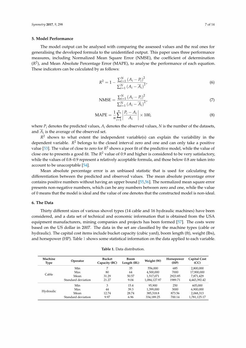
In this study, a new hybrid model is proposed, in which the MVR model and ANNs are integratedto acquire a robust and efficient method for cost estimation of shovel machines. Since the MVR is alinear approach that is unable to recognise nonlinear patterns in data, the ANN is applied to modelthe residuals and to acquire the nonlinear behaviour, while the result of the ANN is added to thefinal output. Therefore, the MVR model will be responsible for the linear model, while the ANN willbe responsible for the nonlinear part. A diagram of the model can be schematically seen in Figure 3.
Having this in mind, we assume that the shovel costs are classed as the nonlinear and linear parts:
Yt = Lt + NLt (5)
where NLt and Lt indicate the nonlinear and linear components, respectively. Therefore, the main ideais to employ, in the first place, the MVR model, and, next, to apply the ANN to formulate the residualsof the linear structure. A schematic diagram of the proposed model is shown in Figure 3.
Symmetry 2017, 9, 298 6 of 13
and to acquire the nonlinear behaviour, while the result of the ANN is added to the final output. Therefore, the MVR model will be responsible for the linear model, while the ANN will be responsible for the nonlinear part. A diagram of the model can be schematically seen in Figure 3.
Having this in mind, we assume that the shovel costs are classed as the nonlinear and linear parts:
= +t t tY L NL (5)
where NLt and Lt indicate the nonlinear and linear components, respectively. Therefore, the main idea is to employ, in the first place, the MVR model, and, next, to apply the ANN to formulate the residuals of the linear structure. A schematic diagram of the proposed model is shown in Figure 3.
Figure 3. The approach used in the research.
Since the MVR model cannot approximate the nonlinear patterns that are involved in the dataset, then the residuals of the linear pattern may comprise nonlinear behaviour, which cannot be captured by a linear pattern. The combination model includes the exceptional advantages of both MVR and ANN models, allowing it to recognise various patterns. Therefore, it is profitable to separately formulate nonlinear and linear patterns by employing multiple patterns and, then, to integrate the results for improving the outcomes and model efficiency.
5. Model Performance
The model output can be analysed with comparing the assessed values and the real ones for generalising the developed formula to the unidentified output. This paper uses three performance measures, including Normalized Mean Square Error (NMSE), the coefficient of determination (R2), and Mean Absolute Percentage Error (MAPE), to analyse the performance of each equation. These indicators can be calculated by as follows:
22 1
21
1 ,−
−−
−
N
i ii=
N
i ii=
(A P )R =
(A A )
(6)
Figure 3. The approach used in the research.
Since the MVR model cannot approximate the nonlinear patterns that are involved in the dataset,then the residuals of the linear pattern may comprise nonlinear behaviour, which cannot be captured bya linear pattern. The combination model includes the exceptional advantages of both MVR and ANNmodels, allowing it to recognise various patterns. Therefore, it is profitable to separately formulatenonlinear and linear patterns by employing multiple patterns and, then, to integrate the results forimproving the outcomes and model efficiency.
Symmetry 2017, 9, 298 7 of 14
5. Model Performance
The model output can be analysed with comparing the assessed values and the real ones forgeneralising the developed formula to the unidentified output. This paper uses three performancemeasures, including Normalized Mean Square Error (NMSE), the coefficient of determination(R2), and Mean Absolute Percentage Error (MAPE), to analyse the performance of each equation.These indicators can be calculated by as follows:
R2 = 1− ∑Ni=1 (Ai − Pi)
2
∑Ni=1 (Ai − Ai)
2 , (6)
NMSE =∑N
i=1 (Ai − Pi)2
∑Ni=1 (Ai − Ai)
2 , (7)
MAPE =1n
n
∑i=1
∣∣∣∣Pi − AiAi
∣∣∣∣× 100, (8)
where Pi denotes the predicted values, Ai denotes the observed values, N is the number of the datasets,and Ai is the average of the observed set.
R2 shows to what extent the independent variable(s) can explain the variability in thedependent variable. R2 belongs to the closed interval zero and one and can only take a positivevalue [53]. The value of close to zero for R2 shows a poor fit of the predictive model, while the value ofclose one to presents a good fit. The R2 value of 0.9 and higher is considered to be very satisfactory,while the values of 0.8–0.9 represent a relatively acceptable formula, and those below 0.8 are taken intoaccount to be unacceptable [54].
Mean absolute percentage error is an unbiased statistic that is used for calculating thedifferentiation between the predicted and observed values. The mean absolute percentage errorcontains positive numbers without having an upper bound [55,56]. The normalized mean square errorpresents non-negative numbers, which can be any numbers between zero and one, while the valueof 0 means that the model is ideal and the value of one denotes that the constructed model is non-ideal.
6. The Data
Thirty different sizes of various shovel types (14 cable and 16 hydraulic machines) have beenconsidered, and a data set of technical and economic information that is obtained from the USAequipment manufacturers, mining companies and projects has been formed [57]. The costs werebased on the US dollar in 2007. The data in the set are classified by the machine types (cable orhydraulic). The capital cost items include bucket capacity (cubic yard), boom length (ft), weight (Ibs),and horsepower (HP). Table 1 shows some statistical information on the data applied to each variable.
Table 1. Data distribution.
MachineType Operator Bucket
Capacity (BC)Boom
Length (BL) Weight (W) Horsepower(HP)
Capital Cost(CC)
Cable
Min 7 35 556,000 685 2,800,000Max 80 64 4,500,000 7000 17,900,000
Mean 31.29 50.57 1,517,071 2923.85 7,871,429Standard deviation 21.27 9.04 1,084,127.97 1989.71 4,443,392.42
Hydraulic
Min 3 15.4 95,900 250 605,000Max 44 39.3 1,399,000 3000 6,900,000
Mean 12.74 28.74 385,318.8 873.56 2,068,313Standard deviation 9.97 6.96 334,189.25 700.14 1,781,125.17
Symmetry 2017, 9, 298 8 of 14
7. The Implementation of the Proposed Model
The 22 data items were randomly used to formulate the model, and, then, other items of the dataset were selected to evaluate the performance of the model. First, by using the MVR model, the linearpattern in the data was extracted as
CC = 1,287,582.06 × D + 129,953.24 × BC + 44,841.31 × BL + 0.12 ×W + 438.241 × HP − 1324,659.59 (9)
Then, the residuals of the MVR model were entered into the neural network as an input.Training minimises the error between the network output and the target output by repeatedly changingthe values of the ANN’s connection weights according to a predetermined algorithm [58].
Different algorithms are developed to model a complex structure that is involved in the dataset.Feed forward back propagation method is the most efficient technique for obtaining good results [59].In this paper, the selected network was based on feedforward backpropagation (as seen in Figure 2).A backpropagation network is a multilinear perceptron that is constructed by three main layers (i) onelayer for connecting independent variables to the formulating system by using nodes, namely inputlayer; (ii) one or more layers for capturing the patterns involved in data by using nodes, namelyintermediate layer(s); and (iii) one layer for connecting dependent variables to the formulating systemwith nodes, namely output layer [60].
Moreover, the training process of the network is fulfilled by utilizing the triangular function,employing the backpropagation algorithm by adjusting the value of weights and bias concerninggradient descent with the momentum, under Matlab software environment.
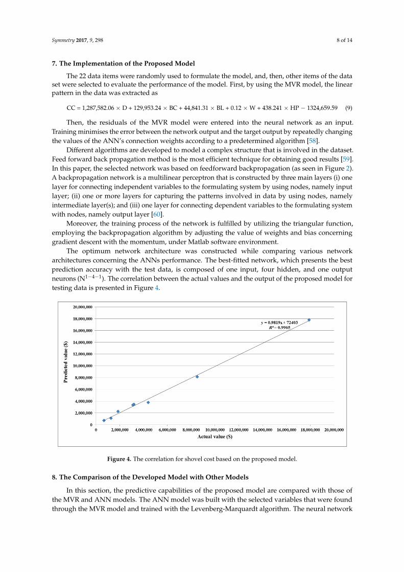
The optimum network architecture was constructed while comparing various networkarchitectures concerning the ANNs performance. The best-fitted network, which presents the bestprediction accuracy with the test data, is composed of one input, four hidden, and one outputneurons (N1−4−1). The correlation between the actual values and the output of the proposed model fortesting data is presented in Figure 4.
Symmetry 2017, 9, 298 8 of 13
Different algorithms are developed to model a complex structure that is involved in the dataset. Feed forward back propagation method is the most efficient technique for obtaining good results [59]. In this paper, the selected network was based on feedforward backpropagation (as seen in Figure 2). A backpropagation network is a multilinear perceptron that is constructed by three main layers (i) one layer for connecting independent variables to the formulating system by using nodes, namely input layer; (ii) one or more layers for capturing the patterns involved in data by using nodes, namely intermediate layer(s); and (iii) one layer for connecting dependent variables to the formulating system with nodes, namely output layer [60].
Moreover, the training process of the network is fulfilled by utilizing the triangular function, employing the backpropagation algorithm by adjusting the value of weights and bias concerning gradient descent with the momentum, under Matlab software environment.
The optimum network architecture was constructed while comparing various network architectures concerning the ANNs performance. The best-fitted network, which presents the best prediction accuracy with the test data, is composed of one input, four hidden, and one output neurons (N1−4−1). The correlation between the actual values and the output of the proposed model for testing data is presented in Figure 4.
Figure 4. The correlation for shovel cost based on the proposed model.
8. The Comparison of the Developed Model with Other Models
In this section, the predictive capabilities of the proposed model are compared with those of the MVR and ANN models. The ANN model was built with the selected variables that were found through the MVR model and trained with the Levenberg-Marquardt algorithm. The neural network model used is composed of five input, eight hidden, and one output neurons (N5−8−1). The results of different models used for testing data are presented in Table 2.
The performance measures of the proposed and other models for testing a data set are presented in Table 3. It can be seen that the NMSE value for the proposed model is 0.0035, which is smaller than those obtained by using MVR and ANN, making 0.0059 and 0.0076, respectively.
The MAPE value for the proposed model is 9.59%, which is also dramatically smaller than those obtained by ANN and MVR, and making 17.44% and 20%, respectively. The R2 value for the proposed model is 0.9965, which is bigger than those that are yielded by MVR and ANN and making 0.9941 and 0.9924, respectively. The experimental results presented in Table 2 show that the hybrid models are more accurate. This conclusion can be derived because the hybrid models integrate linear and nonlinear information for predicting, while the individual model uses only linear or nonlinear information for modeling.
Figure 4. The correlation for shovel cost based on the proposed model.
8. The Comparison of the Developed Model with Other Models
In this section, the predictive capabilities of the proposed model are compared with those ofthe MVR and ANN models. The ANN model was built with the selected variables that were foundthrough the MVR model and trained with the Levenberg-Marquardt algorithm. The neural network
Symmetry 2017, 9, 298 9 of 14
model used is composed of five input, eight hidden, and one output neurons (N5−8−1). The results ofdifferent models used for testing data are presented in Table 2.
Table 2. The comparison of different models.
Case Actual MVR ANN Proposed Model
1 680,000 120,755.6 815,732.3 716,660.32 1,263,000 120,2621 1,299,821 1,115,8283 1,850,000 2,338,051 2,145,405 2,293,9474 4,400,000 3,903,419 5,124,051 3,802,9855 3,200,000 3,528,523 3,719,688 3,470,7806 8,500,000 7,865,014 9,298,305 8,150,0037 3,100,000 3,431,278 4,803,671 3,378,5038 17,900,000 16,661,424 18,551,802 17,801,455
The performance measures of the proposed and other models for testing a data set are presentedin Table 3. It can be seen that the NMSE value for the proposed model is 0.0035, which is smaller thanthose obtained by using MVR and ANN, making 0.0059 and 0.0076, respectively.
Table 3. Performance measures of the proposed model and other models for testing data.
Model R2 NMSE MAPE
Proposed model 0.9965 0.0035 9.59%ANN 0.9924 0.0076 17.44%MVR 0.9941 0.0059 20%
The MAPE value for the proposed model is 9.59%, which is also dramatically smaller thanthose obtained by ANN and MVR, and making 17.44% and 20%, respectively. The R2 value for theproposed model is 0.9965, which is bigger than those that are yielded by MVR and ANN and making0.9941 and 0.9924, respectively. The experimental results presented in Table 2 show that the hybridmodels are more accurate. This conclusion can be derived because the hybrid models integrate linearand nonlinear information for predicting, while the individual model uses only linear or nonlinearinformation for modeling.
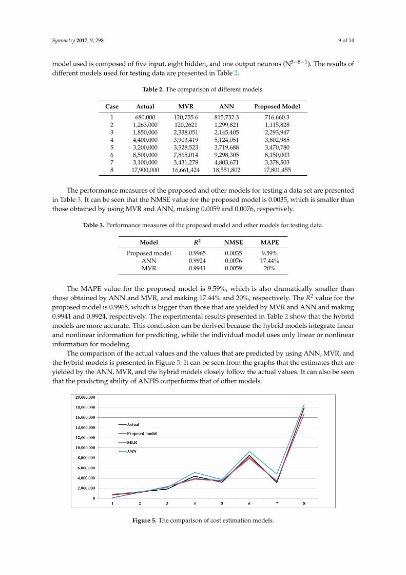
The comparison of the actual values and the values that are predicted by using ANN, MVR, andthe hybrid models is presented in Figure 5. It can be seen from the graphs that the estimates that areyielded by the ANN, MVR, and the hybrid models closely follow the actual values. It can also be seenthat the predicting ability of ANFIS outperforms that of other models.
Symmetry 2017, 9, 298 9 of 13
Table 2. The comparison of different models.
Case Actual MVR ANN Proposed Model 1 680,000 120,755.6 815,732.3 716,660.3 2 1,263,000 120,2621 1,299,821 1,115,828 3 1,850,000 2,338,051 2,145,405 2,293,947 4 4,400,000 3,903,419 5,124,051 3,802,985 5 3,200,000 3,528,523 3,719,688 3,470,780 6 8,500,000 7,865,014 9,298,305 8,150,003 7 3,100,000 3,431,278 4,803,671 3,378,503 8 17,900,000 16,661,424 18,551,802 17,801,455
Table 3. Performance measures of the proposed model and other models for testing data.
Model R2 NMSE MAPE Proposed model 0.9965 0.0035 9.59%
ANN 0.9924 0.0076 17.44% MVR 0.9941 0.0059 20%
The comparison of the actual values and the values that are predicted by using ANN, MVR, and the hybrid models is presented in Figure 5. It can be seen from the graphs that the estimates that are yielded by the ANN, MVR, and the hybrid models closely follow the actual values. It can also be seen that the predicting ability of ANFIS outperforms that of other models.
The obtained result is also in good agreement with the previous studies [8], which state that, in most cases, the accuracy of the estimation by hybrid procedures would be better than that for pure statistical methods due to the essential property of costs, which are cumulative. To facilitate the cost estimation, it is also possible to apply convex optimization algorithms [61,62] and to compare the results in future works.
Figure 5. The comparison of cost estimation models.
9. Sensitivity Analysis
Sensitivity analysis is a useful tool for determining the relationship between the considered parameters [63]. The most sensitive factors affecting the shovel capital cost is analysed by the cosine amplitude method (CAM). This method is a useful tool for performing sensitivity analysis.
Based on the concepts of the CAM method, the sensitivity for each independent component can be determined through establishing the degree of the relationship (rij) between the shovel capital cost and the considered independent component [56]. The larger the value of CAM, the higher its impact
Figure 5. The comparison of cost estimation models.
Symmetry 2017, 9, 298 10 of 14
The obtained result is also in good agreement with the previous studies [8], which state that, inmost cases, the accuracy of the estimation by hybrid procedures would be better than that for purestatistical methods due to the essential property of costs, which are cumulative. To facilitate the costestimation, it is also possible to apply convex optimization algorithms [61,62] and to compare theresults in future works.
9. Sensitivity Analysis
Sensitivity analysis is a useful tool for determining the relationship between the consideredparameters [63]. The most sensitive factors affecting the shovel capital cost is analysed by the cosineamplitude method (CAM). This method is a useful tool for performing sensitivity analysis.
Based on the concepts of the CAM method, the sensitivity for each independent component canbe determined through establishing the degree of the relationship (rij) between the shovel capitalcost and the considered independent component [56]. The larger the value of CAM, the higher itsimpact on the capital cost. If the shovel capital cost is not related to the independent variable, then,the CAM value is zero. The independent variable plays a positive role the shovel capital cost wherethe CAM value is non-negative and plays a negative role in the shovel capital cost where the CAMvalue is non-positive.
Let n be the number of independent variables represented as an array X = {x1, x2, . . . , xn}, whileeach of its elements, xi, in the data array X, is itself a vector of length m, and can be expressed as:
Xi = {xi1, xi2, xi3, . . . , xim}, (10)
Thus, each of the data pairs can be viewed as a point in m dimensional space, where each pointrequires m coordinates for a complete description [64]. Each element of the relation, rij, results from apairwise comparison of two data samples. The strength of the relationship between the data samples,xi and xj, is given by the membership value, expressing this strength:
rij =∑m
k=1 xikxjk√∑m
k=1 X2ik∑m
k=1 X2jk
, 0 ≤ rij ≤ 1. (11)
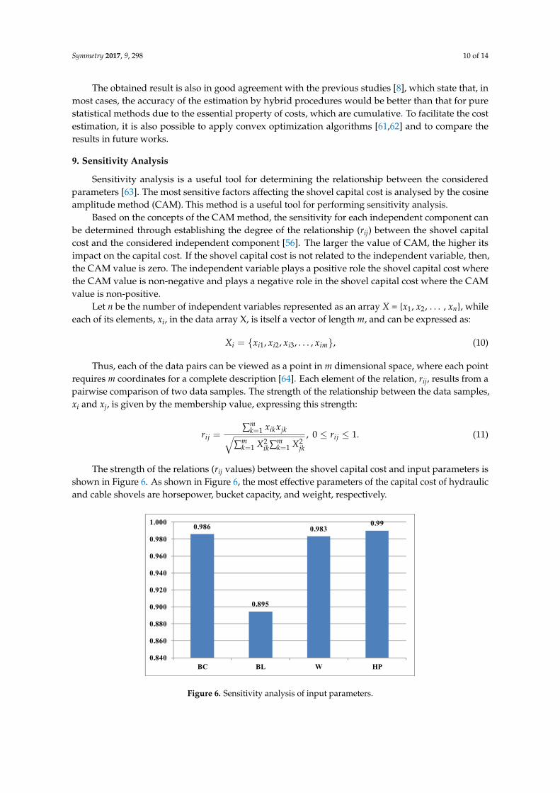
The strength of the relations (rij values) between the shovel capital cost and input parameters isshown in Figure 6. As shown in Figure 6, the most effective parameters of the capital cost of hydraulicand cable shovels are horsepower, bucket capacity, and weight, respectively.
Symmetry 2017, 9, 298 10 of 13
on the capital cost. If the shovel capital cost is not related to the independent variable, then, the CAM value is zero. The independent variable plays a positive role the shovel capital cost where the CAM value is non-negative and plays a negative role in the shovel capital cost where the CAM value is non-positive.
Let n be the number of independent variables represented as an array X = {x1, x2, ..., xn}, while each of its elements, xi, in the data array X, is itself a vector of length m, and can be expressed as:
, (10)
Thus, each of the data pairs can be viewed as a point in m dimensional space, where each point requires m coordinates for a complete description [64]. Each element of the relation, rij, results from a pairwise comparison of two data samples. The strength of the relationship between the data samples, xi and xj, is given by the membership value, expressing this strength:
. (11)
The strength of the relations (rij values) between the shovel capital cost and input parameters is shown in Figure 6. As shown in Figure 6, the most effective parameters of the capital cost of hydraulic and cable shovels are horsepower, bucket capacity, and weight, respectively.
Figure 6. Sensitivity analysis of input parameters.
10. Conclusions
Despite the fact that there are many different prediction models, the improvement of prediction accuracy is still an acute problem that is facing decision makers in many areas. Multivariable regression (MVR) models are among the most popular linear models in predicting. Although various techniques have been widely used with the aim of constructing more accurate models, they cannot recognise nonlinear patterns in the existing data. On the other hand, artificial neural networks (ANNs) are well-known as the useful tools for pattern recognition, clustering, and, mainly, prediction with a high degree of accuracy, but it is hardly reasonable to use the ANNs blindly to model linear problems. The hybrid methods, which decompose a problem into its linear and nonlinear constituent parts, refer to the most efficient models.
In this paper, the hybridisation of the MVR and ANN models is proposed to overcome their limitations mentioned above and to yield a more accurate predictive model that is generated by individual methods. In the proposed model, the unique capability of the MVR model has been utilised in linear modelling to recognise the existing linear structure in data, and, then, an ANN is applied to model the nonlinear forms, using the preprocessed data. The results obtained demonstrate that the proposed model is superior to the individual models regarding three indices, and can yield more accurate data. Moreover, MVR provides the excellent initial approximation of the error due to
{ }1 2 3, , ,...,i i i i imX x x x x=
1
2 21 1
, 0 1m
ik jkkij ijm m
ik jkk k
x xr r
X X
=
= =
= ≤ ≤
0.986
0.895
0.9830.99
0.840
0.860
0.880
0.900
0.920
0.940
0.960
0.980
1.000
BC BL W HP
Figure 6. Sensitivity analysis of input parameters.

Symmetry 2017, 9, 298 11 of 14
10. Conclusions
Despite the fact that there are many different prediction models, the improvement of predictionaccuracy is still an acute problem that is facing decision makers in many areas. Multivariable regression(MVR) models are among the most popular linear models in predicting. Although various techniqueshave been widely used with the aim of constructing more accurate models, they cannot recognisenonlinear patterns in the existing data. On the other hand, artificial neural networks (ANNs) arewell-known as the useful tools for pattern recognition, clustering, and, mainly, prediction with a highdegree of accuracy, but it is hardly reasonable to use the ANNs blindly to model linear problems.The hybrid methods, which decompose a problem into its linear and nonlinear constituent parts, referto the most efficient models.
In this paper, the hybridisation of the MVR and ANN models is proposed to overcome theirlimitations mentioned above and to yield a more accurate predictive model that is generated byindividual methods. In the proposed model, the unique capability of the MVR model has been utilisedin linear modelling to recognise the existing linear structure in data, and, then, an ANN is appliedto model the nonlinear forms, using the preprocessed data. The results obtained demonstrate thatthe proposed model is superior to the individual models regarding three indices, and can yield moreaccurate data. Moreover, MVR provides the excellent initial approximation of the error due to nonlinearpart as the initial data of the ANN. Therefore, this fact enables the reduction computation time ofthe ANN.
It should be noted that the proposed methodology could be only employed for complex systems.Therefore, it is appropriate for a dataset with at least one nonlinear pattern that is involvedin information.
Author Contributions: The individual contribution and responsibilities of the authors were as follows:Abdolreza Yazdani-Chamzini and Edmundas Kazimieras Zavadskas designed the research,Abdolreza Yazdani-Chamzini collected and analyzed the data and the obtained results, performed thedevelopment of the paper. Edmundas Kazimieras Zavadskas, Jurgita Antucheviciene and Romualdas Bausysprovided extensive advice throughout the study, regarding the research design, methodology, findings andrevised the manuscript. All the authors have read and approved the final manuscript.
Conflicts of Interest: The authors declare no conflict of interest.
References
1. Devi, L.P.; Palaniappan, S. A study on energy use for excavation and transport of soil during buildingconstruction. J. Clean. Prod. 2017, 164, 543–556. [CrossRef]
2. Atkinson, T. Selection and sizing of excavating equipment. In SME Mining Engineering Handbook; Society forMining, Metallurgy, and Exploration: Littleton, CO, USA, 1992; pp. 1311–1333.
3. Tatiya, R.R. Surface and Underground Excavations—Methods, Techniques and Equipment; Taylor & FrancisGroup plc: London, UK, 2005.
4. Huang, J.; Dong, Z.; Quan, L.; Jin, Z.; Lan, Y.; Wang, Y. Development of a dual displacement controlledcircuit for hydraulic shovel swing motion. Autom. Constr. 2015, 57, 166–174. [CrossRef]
5. Elevli, S.; Elevli, B. Performance measurement of mining equipments by utilizing OEE. Acta Montan. Slovaca2010, 15, 95–101.
6. Lashgari, A.; Yazdani-Chamzini, A.; Fouladgar, M.M.; Zavadskas, E.K.; Shafiee, S.; Abbate, N. Equipmentselection using fuzzy multi criteria decision making model: Key study of Gole Gohar iron mine. Inz. Econ.2012, 23, 125–136. [CrossRef]
7. Sayadi, A.R.; Lashgari, A.; Fouladgar, M.M.; Skibniewski, M. Estimating capital and operational costs ofbackhoe shovels. J. Civ. Eng. Manag. 2012, 18, 378–385. [CrossRef]
8. Mutmansky, J.M.; Suboleski, S.C.; O’Hara, T.A.; Prasad, K.V.K. Cost comparisons. In SME Mining EngineeringHandbook, 2nd ed.; Hartman, H.L., Ed.; Society for Mining, Metallurgy, and Exploration: Littleton, CO, USA,1992; pp. 2070–2089.
9. Anon. Estimating Preproduction and Operating Costs of Small Underground Deposits (CANMET); CanadianGovernment Publishing Centre: Ottawa, ON, Canada, 1986.
Symmetry 2017, 9, 298 12 of 14
10. Mular, A.L.; Poulin, R. CAPCOSTS: A Handbook for Estimating Mining and Mineral Processing Equipment Costsand Capital Expenditures and Aiding Mineral Project Evaluations; CIM Bulletin Special, 47; Canadian Institute ofMining and Metallurgy: Montréal, QC, Canada, 1998.
11. Mular, A.L. Mining and Mineral Processing Equipment Costs and Preliminary Capital Cost Estimation; CIM BulletinSpecial, 25; Canadian Institute of Mining and Metallurgy: Montreal, QC, Canada, 1982.
12. Lanz, T.; Noakes, M. Cost Estimation Handbook for the Australian Mining Industry; Australasian Institute ofMining and Metallurgy (Aus IMM): Carlton South, Australia, 1993.
13. USBM. US Bureau of Mines Cost Estimating System Handbook, Mining and Beneficiation of Metallic and NonmetallicMinerals Expected Fossil Fuels in the United States and Canada; United States Bureau of Mines: Denver, CO,USA, 1987; pp. 10–87.
14. Mohutsiwa, M.; Musingwini, C. Parametric estimation of capital costs for establishing a coal mine: SouthAfrica case study. J. South. Afr. Inst. Min. Metall. 2015, 115, 789–797. [CrossRef]
15. Sayadi, A.R.; Lashgari, A.; Paraszczak, J. Hard-rock LHD cost estimation using single and multipleregressions based on principal component analysis. Tunn. Undergr. Space Technol. 2012, 27, 133–141.[CrossRef]
16. O’Hara, T.A. Quick guide to the evaluation of ore bodies. CIM Bull. 1998, 88, 34–43.17. O’Hara, T.A. Mine Evaluation, Mineral Industry Costs; Hoskins, J.R., Ed.; Northwest Mining Association:
Spokane, WA, USA, 1982; pp. 89–99.18. O’Hara, T.A. Quick Guide to Mine Operating Costs and Revenue; Paper No. 186; CIM Annual General Meeting:
Toronto, ON, Canada, 1987.19. O’Hara, T.A.; Suboleski, C.S. Costs and Cost Estimation. In SME Mining Engineering Handbook; Society for
Mining, Metallurgy, and Exploration: Littleton, CO, USA, 1992; Volume 1, pp. 405–424.20. Camm, T.W. Simplified cost models for pre-feasibility mineral evaluations. Min. Eng. 1994, 46, 559–562.21. Rudenno, V. The Mining Valuation Handbook: Australian Mining and Energy Valuation for Investors and
Management; Australian Print Group: Victoria, Australia, 1998.22. Sayadi, A.R.; Khademi, J.; Rahimi, M.A. Estimating the energy costs of mine equipment using an information
system. In Proceedings of the 24th International Mining Congress and Exhibition of Turkey, Antalya, Turkey,14–17 April 2015; pp. 9–18.
23. Wei, Y.; Qiu, J.; Shi, P.; Chadli, M. Fixed-order piecewise-affine output feedback controller forfuzzy-affine-model-based nonlinear systems with time-varying delay. IEEE Trans. Circuits Syst. I Regul. Pap.2017, 64, 945–958. [CrossRef]
24. Wei, Y.; Qiu, J.; Karimi, H.R. Fuzzy-affine-model-based memory filter design of nonlinear systems withtime-varying delay. IEEE Trans. Fuzzy Syst. 2017, PP, 1. [CrossRef]
25. Singh, V.; Gupta, I.; Gupta, H.O. ANN-based estimator for distillation using Levenberg-Marquardt approach.Eng. Appl. Artif. Intell. 2007, 20, 249–259. [CrossRef]
26. Yamamura, S. Clinical application of artificial neural network (ANN) modeling to predict pharmacokineticparameters of severely ill patients. Adv. Drug Deliv. Rev. 2003, 55, 1233–1251. [CrossRef]
27. Lian-Guo, W.; Zhi-Kang, Z.; Yin-Long, L.; Hong-Bo, Y.; Sheng-Qiang, Y.; Jian, S.; Jin-Yao, Z. Combined ANNprediction model for failure depth of coal seam floors. Min. Sci. Technol. 2009, 19, 684–688.
28. Fast, M.; Assadi, M.; De, S. Development and multi-utility of an ANN model for an industrial gas turbine.Appl. Energy 2009, 86, 9–17. [CrossRef]
29. Lee, J.; Sanmugarasa, K.; Blumenstein, M.; Loo, Y.C. Improving the reliability of a Bridge ManagementSystem (BMS) using an ANN-based Backward Prediction Model (BPM). Autom. Constr. 2008, 17, 758–772.[CrossRef]
30. Jalali-Heravi, M.; Asadollahi-Baboli, M.; Mani-Varnosfaderani, A. Shuffling multivariate adaptive regressionsplines and adaptive neuro-fuzzy inference system as tools for QSAR study of SARS inhibitors. J. Pharm.Biomed. Anal. 2009, 50, 853–860. [CrossRef] [PubMed]
31. Verlinden, B.; Duflou, J.R.; Collin, P.; Cattrysse, D. Cost estimation for sheet metal parts using multipleregression and artificial neural networks: A case study. Int. J. Prod. Econ. 2008, 111, 484–492. [CrossRef]
32. Mesroghli, S.; Jorjani, E.; Chelgani, S.C. Estimation of gross calorific value based on coal analysis usingregression and artificial neural networks. Int. J. Coal Geol. 2009, 79, 49–54. [CrossRef]
33. Sahoo, G.B.; Schladow, S.G.; Reuter, J.E. Forecasting stream water temperature using regression analysis,artificial neural network, and chaotic non-linear dynamic models. J. Hydrol. 2009, 378, 325–342. [CrossRef]
Symmetry 2017, 9, 298 13 of 14
34. Gu, Y.; Wu, L.; Tang, S. A fuzzy neutral-network-driven weighting system for electric shovel. In Advances inNeural Networks—ISNN 2008; Sun, F., Zhang, J., Tan, Y., Cao, J., Yu, W., Eds.; Lecture Notes in ComputerScience; Springer: Berlin/Heidelberg, Germany, 2008; Volume 5264, pp. 526–532.
35. Guo, J.; Zhao, X.; Guo, J.; Yuan, X.; Dong, S.; Xiong, Z. Model updating of suspended-dome using artificialneural networks. Adv. Struct. Eng. 2017, 20, 1727–1743. [CrossRef]
36. Du, Y.; Chen, Z.; Zhang, C.; Cao, X. Research on axial bearing capacity of rectangular concrete-filled steeltubular columns based on artificial neural networks. Front. Comput. Sci. 2017, 11, 863–873. [CrossRef]
37. Gardner, B.J.; Gransberg, D.D.; Rueda, J.A. Stochastic conceptual cost estimating of highway projects tocommunicate uncertainty using bootstrap sampling. ASCE-ASME J. Risk Uncertain. Eng. Part A Civ. Eng.2017, 3. [CrossRef]
38. El-Gohary, K.M.; Aziz, R.F.; Abdel-Khalek, H.A. Engineering approach using ANN to improve and predictconstruction labor productivity under different influences. J. Constr. Eng. Manag. 2017, 143. [CrossRef]
39. Cao, M.S.; Pan, L.X.; Gao, Y.F.; Novak, D.; Ding, Z.C.; Lehky, D.; Li, X.L. Neural network ensemble-basedparameter sensitivity analysis in civil engineering systems. Neural Comput. Appl. 2017, 28, 1583–1590.[CrossRef]
40. Abdeljaber, O.; Avci, O.; Kiranyaz, S.; Gabbouj, M.; Inman, D.J. Real-time vibration-based structural damagedetection using one-dimensional convolutional neural networks. J. Sound Vib. 2017, 388, 154–170. [CrossRef]
41. Benali, A.; Boukhatem, B.; Hussien, M.N.; Nechnech, A.; Karray, M. Prediction of axial capacity of pilesdriven in non-cohesive soils based on neural networks approach. J. Civ. Eng. Manag. 2017, 23, 393–408.[CrossRef]
42. Yousefi, V.; Yakhchali, S.H.; Khanzadi, M.; Mehrabanfar, E.; Šaparauskas, J. Proposing a neural networkmodel to predict time and cost claims in construction projects. J. Civ. Eng. Manag. 2016, 22, 967–978.[CrossRef]
43. Ustinovichius, L.; Peckiene, A.; Popov, V. A model for spatial planning of site and building using BIMmethodology. J. Civ. Eng. Manag. 2017, 23, 173–182. [CrossRef]
44. Wang, W.C.; Bilozerov, T.; Dzeng, R.J.; Hsiao, F.Y.; Wang, K.C. Conceptual cost estimations using neuro-fuzzyand multi-factor evaluation methods for building projects. J. Civ. Eng. Manag. 2017, 23, 1–14. [CrossRef]
45. Monjezi, M.; Rezaei, M.; Varjani, A.Y. Prediction of rock fragmentation due to blasting in Gol-E-Gohar ironmine using fuzzy logic. Int. J. Rock Mech. Min. Sci. 2009, 46, 1273–1280. [CrossRef]
46. Bourquin, J.; Schmidli, H.; Hoogevest, P.; Leuenberger, H. Advantages of Artificial Neural Networks (ANNs)as alternative modelling technique for data sets showing non-linear relationships using data from a galenicalstudy on a solid dosage form. Eur. J. Pharm. Sci. 1998, 7, 5–16. [CrossRef]
47. Malinowski, P.; Ziembicki, P. Analysis of district heating network monitoring by neural networksclassification. J. Civ. Eng. Manag. 2006, 12, 21–28.
48. He, X.; Xu, S. Process Neural Networks Theory and Applications; Springer: Berlin/Heidelberg, Germany, 2007.49. Engelbrecht, A.P. Computational Intelligence: An Introduction; John Wiley & Sons, Ltd.: Hoboken, NJ, USA, 2002.50. Sumathi, S.; Paneerselvam, S. Computational Intelligence Paradigms: Theory & Applications Using MATLAB;
Taylor and Francis Group, LLC: Oxford, UK, 2010.51. Khashei, M.; Bijari, M. A novel hybridization of artificial neural networks and ARIMA models for time series
forecasting. Appl. Soft Comput. 2011, 11, 2664–2675. [CrossRef]52. Zhang, G.P. Time series forecasting using a hybrid ARIMA and neural network model. Neurocomputing 2003,
50, 159–175. [CrossRef]53. Farid, M.; Hossein Abadi, M.M.; Yazdani-Chamzini, A.; Yakhchali, S.H.; Basiri, M.H. Developing a new
model based on neuro-fuzzy system for predicting roof fall in coal mines. Neural Comput. Appl. 2013, 23,129–137. [CrossRef]
54. Nash, J.E.; Sutcliffe, J.V. River flow forecasting through conceptual models, I. A discussion of principles.J. Hydrol. 1970, 10, 282–290. [CrossRef]
55. Razani, M.; Yazdani-Chamzini, A.; Yakhchali, S.H. A novel fuzzy inference system for predicting roof fallrate in underground coal mines. Saf. Sci. 2013, 55, 26–33. [CrossRef]
56. Yazdani-Chamzini, A.; Yakhchali, S.H.; Volungeviciene, D.; Zavadskas, E.K. Forecasting gold price changesby using adaptive network fuzzy inference system. J. Bus. Econ. Manag. 2012, 13, 994–1010. [CrossRef]
57. Info Mine: Mining Cost Service Indexes. Available online: http://www.infomine.com (accessed on 26 June 2015).
Symmetry 2017, 9, 298 14 of 14
58. Wang, W.; Van Gelder, P.H.A.J.M.; Vrijling, J.K.; Ma, J. Forecasting daily streamflow using hybrid ANNmodels. J. Hydrol. 2006, 324, 383–399. [CrossRef]
59. Srinivas, Y.; Raj, A.S.; Oliver, D.H.; Muthuraj, D.; Chandrasekar, N. A robust behavior of Feed forward backpropagation algorithm of Artificial Neural Networks in the application of vertical electrical sounding datainversion. Geosci. Front. 2012, 3, 729–736. [CrossRef]
60. Basheer, I.A.; Hajmeer, M. Artificial neural networks: Fundamentals, computing, design, and application.J. Microbiol. Methods 2000, 43, 3–31. [CrossRef]
61. Wei, Y.; Qiu, J.; Karimi, H.R.; Ji, W. A novel memory filtering design for semi-Markovian jump time-delaysystems. IEEE Trans. Syst. Man Cybern. 2017, PP, 1–13. [CrossRef]
62. Qiu, J.; Wei, Y.; Karimi, H.R.; Gao, H. Reliable Control of Discrete-Time Piecewise-Affine Time-Delay Systemsvia Output Feedback. IEEE Trans. Reliab. 2017, 57, 1491–1550. [CrossRef]
63. Ross, T.J. Fuzzy Logic with Engineering Applications, 3rd ed.; John Wiley & Sons Ltd.: Hoboken, NJ, USA, 2010.64. Yazdani-Chamzini, A.; Razani, M.; Yakhchali, S.H.; Zavadskas, E.K.; Turskis, Z. Developing a fuzzy model
based on subtractive clustering for road header performance prediction. Autom. Constr. 2013, 35, 111–120.[CrossRef]
© 2017 by the authors. Licensee MDPI, Basel, Switzerland. This article is an open accessarticle distributed under the terms and conditions of the Creative Commons Attribution(CC BY) license (http://creativecommons.org/licenses/by/4.0/).