A model for optimizing the assembly and disassembly of electronic

IEEE TRANSACTIONS ON ELECTRONICS PACKAGING MANUFACTURING, VOL. 22, NO. 2, APRIL 1999 105

A Model for Optimizing the Assemblyand Disassembly of Electronic Systems

Peter A. Sandborn,Member, IEEE,and Cynthia F. Murphy

Abstract—This paper presents a methodology that incorporatessimultaneous consideration of economic and environmental meritduring the virtual prototyping phase of electronic product design.A model that allows optimization of a product life cycle, whichincludes primary assembly, disassembly, and secondary assemblyusing a mix of new and salvaged components, is described.Optimizing this particular life cycle scenario is important forproducts that are leased to customers or subject to producttake-back laws. Monte Carlo simulation is used to account foruncertainty in the data, and demonstrates that high-level designand process decisions may be made with a few basic metricsand without highly specific data sets for every material andcomponent used in a product. A web-based software tool hasbeen developed that implements this methodology.

Index Terms—Design-for-environment, design-to-cost, disas-sembly, electronics product take-back, end of life, recycling,virtual prototyping.

NOMENCLATURE

Quantities associated with specific process steps and the entireunit assembly:

Buy back fraction Fraction of the primary assemblycost paid to reacquire primary as-semblies for recovery (per assem-bly).

Cost Cost of performing a single assem-bly process step (per unit assem-bly).

Cost Allocated buy back cost (per as-sembly).

Cost Cumulative cost of all precedingassembly and test steps (per unitassembly).

Cost Cost of manufacturing the primaryassembly (per unit assembly).

Cost Cost of performing a single teststep (per unit assembly).

Fraction returned Fraction of the primary unit assem-blies returned for recovery that aresalvageable.

Manuscript received August 31, 1998; revised February 5, 1999.P. A. Sandborn is with CALCE Electronic Products and Systems Center,

University of Maryland, College Park, MD 20742 USA.C. F. Murphy is with Microelectronics and Computer Technology Corpo-

ration (MCC), Austin, TX 78759 USA.Publisher Item Identifier S 1521-334X(99)05845-0.

Number of primaryunit assemblies Total number of primary unit as-

semblies to be manufactured.Number of secondary

unit assemblies Total number of secondary unit as-semblies to be manufactured.

Pass fraction Fraction of unit assemblies that arepassed by a test step.

Quality Cumulative probability of defectsnot being introduced to the unit as-sembly as a result of all precedingassembly steps.

Quality Probability that the unit assemblyis not defective at the conclusionof an assembly step.

Scrap Fraction of unit assemblies en-tering the th test step that arescrapped by the th test step.

ScrapCum Cumulative fraction of the unit as-semblies that started the assemblyprocess that have been scrappedafter the th test step.

Secondary build ratio Ratio of secondary to primary unitassemblies manufactured.

Test effectiveness Probability of a test step accuratelyidentifying a defect in a part or unitassembly.

Used Cumulative material used by allpreceding process steps (per unitassembly).

Used Material used by one assembly step(per unit assembly).

Waste Total material wasted after a teststep (per unit assembly).

Waste Total material wasted prior to a teststep (per unit assembly).

Waste Material wasted by one assemblystep (per unit assembly).

Quantities associated with specific parts (compo-nents/subcomponents of the unit assembly):

Cost Cost of attaching a single instanceof a part.

Cost Cost of a single instance of a new(not salvaged) part.

Cost Cost of testing a single instanceof a part.

1521–334X/99$10.00 1999 IEEE

106 IEEE TRANSACTIONS ON ELECTRONICS PACKAGING MANUFACTURING, VOL. 22, NO. 2, APRIL 1999

CostAvg Average cost per single instanceof a part (combination of new andsalvaged parts).

CostAvg Average cost per single instanceof a part recovered from salvagedunit assemblies.

Defects Probability of a defect occurringwhen attaching a single instanceof a part to the assembly.Fraction of parts in the secondaryassembly that came from salvagedprimary assemblies.

Pass fraction Fraction of salvaged parts that arepassed by a test step.

Quality Probability that the current disas-sembly step does not produce adefect in the part being removed.

Quality Cumulative probability of defectsnot being introduced to a part ateach of the preceding assemblysteps.

Quality Probability that a new part is notdefective.

Quality Probability that a component isnot defective after primary life,prior to disassembly.

Quality Probability that a component isnot defective after primary life,prior to disassembly.

QualityAvg Average probability that a part isnot defective (combination of newand salvaged parts).

QualityAvg Average probability that a part re-covered from a primary assemblyand retested is not defective.

Quantity Quantity (number of instances) ofa specific part assembled by anassembly step.

Used Material used when attaching oneinstance of a part.

Used Material used when fabricatingone instance of a part.

UsedAvg Average material used when in-cluding one instance of a part inthe unit assembly.

Waste Material wasted when attachingone instance of a part.

Waste Material wasted when fabricatingone instance of a part.

WasteAvg Average material wasted when in-cluding one instance of a part inthe unit assembly.

1These quantities are the effective quantities per part, averaged over a largenumber of parts. New and salvaged parts are assumed to be tested to the samequality level.

I. INTRODUCTION

M OST products are optimized for manufacturability, andcosts are minimized under the assumption of only a

single or “primary” life. When the primary life of the productis over, the original equipment manufacturer (OEM) of theproduct is rarely involved with the product again. With theadvent of more stringent product take-back laws in Europeand those on the horizon in the United States [1], OEM’s ofmany products are being forced to contend with a significantpercentage of the products being returned to the OEM at theend of the product’s primary life. OEM’s also contend with thereturn of products when the product is leased to the customerfor a finite period of time. Under these circumstances, theOEM must consider the cost associated with end of life (EOL)scenarios when performing design tradeoffs and consideringthe product’s life cycle costs. Possible EOL scenarios includeresale, remanufacturing, recycling, disposal, and refurbishing.

An increasing number of products are being designed withthe secondary lives taken into account, e.g., photocopiers[2], telephones, video cassettes recorders, and televisions [3].For the purposes of the analysis presented here, a secondarylife is considered to be the reuse of some or all of thecomponents in the primary assembly to build a second iden-tical product; any of the primary components that are notreused in the secondary assembly are disposed of. The uni-versal application of this approach, not considered in thispaper, is the reuse of components in many products includingidentical, similar, or perhaps significantly different products.The challenge is to determine, on an application specificbasis, what subset of components should be reused and whatsubset should be disposed of in order to minimize systemcosts. Several interdependent issues must be considered toproperly determine the optimum component reuse scenario,including assembly costs, disassembly costs; defects intro-duced in the assembly, disassembly, and primary life use ofthe product; and the waste stream associated with the lifecycle.

Two bodies of existing work are relevant to this paper.The first focuses on cost modeling associated with EOLstrategies and the second is aimed at production planningand inventory control. EOL strategies that involve disassemblyhave been modeled many different ways. Approaches include,“scorecards” [4]; life cycle assessment (LCA) [5]; cost-benefitanalysis [6]; activity-based costing (ABC) [7]; decision trees[8]; and high-level financial models [9]. An excellent review ofdisassembly analysis methods appears in [4]. All of these ap-proaches have merit and have been successfully demonstrated.With the exception of financial models, these methods areusually applied to the disassembly process in isolation, i.e., noattempt is made to concurrently model the primary assemblyand the EOL approach to optimize over a broader portion ofthe product life cycle. In the case of financial models, the entirelife cycle is modeled, however, the assembly, disassembly, andtesting costs are often characterized as single values, and themodels do not include a treatment of specific component yieldsor address how the component yields are modified by primaryuse or disassembly processes.

SANDBORN AND MURPHY: OPTIMIZING THE ASSEMBLY AND DISASSEMBLY OF ELECTRONIC SYSTEMS 107

TABLE IINPUTS TO THE MODEL

The second class of existing work falls at the opposite endof the spectrum from the EOL cost models summarized above.These models treat the broader product life cycle, but at theexpense of application-specific manufacturing and disassemblydetails. Several authors have developed rigorous models forproduction/inventory systems that include remanufacturingand disposal, for examples see [10] and [11]. The relevantconcepts included in these efforts are their concurrent treat-ment of primary product manufacturing and remanufacturing,and the inclusion of production issues such as inventory levels,ordering information, time value of money, and lead time.

In the model presented in this paper, actual process modelsthat automatically adapt to changes in component mix andcomponent yields are used for assembly and disassemblymodeling. In addition, material use and waste inventories aregenerated as a result of the process models. The model inthis paper also optimizes over the entire primary assembly,disassembly, and secondary assembly life cycle. The objectiveof the model presented herein is similar to the work presentedin [3]; however, this model is specifically designed to optimizecomponent selection. We suggest that the work presented inthis paper provides application-specific manufacturing cost,yield, and waste input to the existing high-level financial andcost-benefit models for “remanufacture” EOL scenarios, or asthe core of a production/inventory model.

The methodology and model presented in this paper aretargeted for use during “virtual prototyping” of electronicproducts. Virtual prototyping takes place at the earliest phasesof the system design, prior to the start of traditional CADactivities [12]. Virtual prototyping starts with requirementsand constraints, and results in a system specification forhow to build the system (bill of materials, technologies,design rules, and materials). One of the characteristics of thevirtual prototyping phase of the design process is that detaileddescriptive data about the product and the manufacturingprocesses associated with creating it are not well defined. Toobtain meaningful results, we use a Monte Carlo modelingapproach that accommodates the characterization of inputdata as probability distributions. As a result, the outputs

obtained from the models are also probability distributions.This approach allows us to draw valid design conclusionsfrom uncertain design inputs.

II. M ODEL

The model used for this analysis considers four stages inthe life cycle of a product:

1) material and component acquisition;2) primary assembly and test of the product using all new

parts;3) return and disassembly of the product after primary use;4) secondary assembly and test of an identical product

using a mixture of salvaged and new parts.

A. Formulation

The basic inputs to the model are listed in Table I. Thesecondary assembly uses the same process inputs as theprimary assembly process.

The outputs of the model are cost, quality (yield), theamount of waste material generated, and the amount of mate-rial contained in the product. Standard accounting methods areused to accumulate cost and quality through the primary as-sembly processes. Test and/or inspection steps in the assemblyprocesses are characterized by test efficiencies that account fortest escapes (defective parts that are not identified during test).In addition, defects introduced to components, other than thecomponent being disassembled, at each disassembly processstep can be modeled. If, for example, one part is salvaged onlyby destroying another, the probability of introducing defectsto the destroyed part during disassembly would be 100%.

After completion of the disassembly process, componentsmay either be disposed of, or salvaged and used in a secondarybuild of the product. The secondary assembly uses salvagedcomponents supplemented with new components, the mix ofwhich is driven by:

2 In this model, we assume that the test activities do not erroneously rejectgood parts.


1) the ratio of the quantity of secondary products built tothe number of original (primary) products built;

2) the fraction of the original product which is availablefor salvage;

3) the fraction of each individual component that are suc-cessfully salvaged during the disassembly process.

The cost and quality associated with a primary or secondarycomponent assembly step are given by the following relations.Assuming only one type of part is attached per process step, thecost of an assembly process step associated with a componentis

Cost (Quantity)(Cost CostAvg

(1)

The cost of the partCostAvg being assembled in (1)is either Cost (primary assembly) or is given by (2)for the secondary assembly

CostAvg (Cost

(CostAvg (2)

where is the fraction of parts in the secondary assemblythat came from salvaged primary assembliesis derivedbelow). In this model, the cost of a part salvaged from arecovered primary assembly and retested is only the cost oftesting a single instance of the partCost i.e., it doesnot contain a component cost. This is appropriate because,the cost of obtaining the entire used primary assembly fromthe customer and performing all required disassembly is usedas the starting point for the secondary assembly process andcontained within this cost is the cost of obtaining individualsalvaged components. Note, even if the OEM purchases thecomponents of interest back from an asset manager or broker,the broker sets the price of the salvaged component basedon obtaining the whole assembly from the customer andperforming the disassembly.

The fraction of parts in the secondary assembly that comefrom salvaged primary assemblies is computed using

fraction returned pass fraction

secondary build ratio(3)

Where “min” indicates that the smaller of the two quantitieswithin the brackets in (3) is used. As denoted in (3), the valueof is not allowed to exceed one, i.e., it is assumed that takeback is not legislated, and therefore, products whose parts arenot required for secondary assemblies are not bought backor disassembled. The ratio of secondary to primary builds isgiven by

secondary build rationumber of secondary unit assembliesnumber of primary unit assemblies

(4)

The formulations of (3) and (4) are most accurate for matureproducts with constant annual production or products withshort primary lives ( year), i.e., the approximations areless accurate for products whose annual production rates vary

significantly and whose primary lives are multiple years. Thefraction of salvaged parts that pass the test is given by

pass fraction

Quality Quality

Quality (5)

where the interpretation of test effectiveness is the probabilityof the test or inspection activity successfully identifying adefect in a part.

The assembly cost for the primary build is computed usingonly (1). Equations (1)–(5) are used to compute the cost of aprocess step that assembles a component to the system duringthe secondary build.

The quality of the system after an assembly step is given by

Quality QualityAvg

Defects (6)

During the primary assembly, the part qualityQualityAvg is given by Quality the

probability that a new component is not defective. During thesecondary assembly, the part quality is given by

QualityAvg Quality

QualityAvg (7)

The quality of a part salvaged from a recovered primaryassembly and retested is given by

QualityAvg

Quality Quality

Quality (8)

We also have a need to accumulate materials that are part ofthe product and materials that are wasted during the fabricationand assembly processes. We inventory the materials in theproduct and the material wasted and normalize the inventoryto a single product. The quantity of material used and wastedby a process step is given by

Used Quantity UsedAvg Used (9a)

Waste Quantity WasteAvg Waste

(9b)

The material added to the product for a part in (9a) is either(primary assembly) or is given by (10a) for

the secondary assembly. Equation (10b) gives the analogousrelations for material waste

UsedAvg Used (10a)

WasteAvg Waste (10b)

Note, unlike (2), (10) contains no second term multiplied bythe fraction of salvaged parts. In (10), all materials used in, or

3The quality predicted by (8) is higher than the quality intuitively foundif the test effectiveness referred to the probability that defective parts areidentified by the test, instead of the probability that defects are identifiedby the tests. Equation (8) is derived by accounting for the possibility that adefective part could have more than one defect, but that the identification ofany defects, not necessarily all defects, is enough to scrap the part, see [13].


wasted by, fabricating a salvaged part were already accountedfor in the primary assembly the first time the part was acquired.

Test operations during assembly have a unique effect onthe cost, quality, and waste materials (they do not affect thematerials used per assembly). The effective cost of a test step(per unit assembly) is given by

CostCost Cost

pass faction(11)

where is the cumulative cost of the assemblyup to but not including the test step. The pass fraction appearsin the denominator of (11) so that all the money spent onassemblies that do not pass the test is properly reallocated overthe assemblies that pass the test. The fraction of assembliesthat are passed by a test operation is similar to (5)

pass fraction

Quality (12)

The quality of assemblies passed by the test step is given by

Quality Quality

(13)

Test steps do not modify the material content of the assembly,i.e., they neither add nor remove material from assemblies thatthey pass. However, since test steps scrap defective assemblies,the materials in the scrapped assemblies must be reallocatedover the waste inventories associated with all the passedassemblies that continue through the process. The total wasteper assembly is modified in the following way,

Waste

Waste

Used (14)

It is also useful to accumulate the fraction of assemblies thatbegin the assembly process that are scrapped by test stepsthroughout the process. The fraction of assemblies entering the

th test step that are scrapped by theth test step is given by

Scrap pass fraction (15)

The cumulative scrap after theth test step is given by

ScrapCum ScrapCum Scrap

ScrapCum (16)

ScrapCum represents the fraction of the assemblies thatstarted the assembly process that have been scrapped afterthe th test step.

The model is not presently designed to accommodate reworkprocesses. A rework operation that followed a test step wouldrepair some of the scrapped assemblies, resulting in a costrebate and a reduction in the waste allocated to each assembly.

Buy back cost is defined as the cost of obtaining the usedprimary assembly from the customer. It is a combination ofpossible payment to the customer and any administrative orhandling costs required to obtain the primary assembly andreturn it to the factory. Two buy back options are presently

supported. The model will either assume that every primaryassembly is repurchased, or that only the number of primaryassemblies necessary to accommodate the desired numberof secondary assemblies are repurchased. In the first case(all primaries repurchased), the allocated buy back cost perassembly is given by

Costbuy back fraction Cost

secondary build ratio(17a)

if only the minimum number of primary assemblies arerepurchased

Costbuy back fraction Cost

fraction returned(17b)

Cost is added to the disassembly cost associated witha single primary assembly and used as the starting cost for asecondary assembly.

The model, as currently constructed, assumes that the pri-mary and secondary builds are identical products. Whilenot shown or discussed here, the model could easily berestructured to accommodate a secondary build that producesa similar or a completely different product.

B. Uncertainty Analysis

The target for the model presented in this paper is the“virtual prototyping” of an electronic product or system.Virtual prototyping is performed at the earliest phases of thedesign process before detailed physical design (layout androuting) is done, and inputs are often little more than a bill ofmaterials and packaging technology choices. Because minimalinformation is available at this point in the design, and theinformation that is available includes substantial uncertainties,a careful treatment of those uncertainties is necessary to obtainmeaningful analysis results.

In order to facilitate making design and process decisionswith only a few basic metrics and without highly specific datainput sets for every material and component used in a product,the present model treats uncertainties by allowing each input tothe equations outlined in the previous section to be optionallyrepresented as a probability distribution rather than a singlefixed value. Supported distributions include normal, lognor-mal, triangular, and uniform. For example, in the case of thequality of an incoming part, experience with the supplier andthe part suggests a most likely value for the incoming yield, butdifferent shipments of parts may have yields that are slightlyhigher or lower. If distributed values are entered, a MonteCarlo analysis is performed. During the analysis, the modelwill randomly select values within the defined distributionsfor a specified number of samples, or as many samples as arenecessary to meet a specified confidence level.

A triangular distribution (Fig. 1) is included as an optionbecause both the minimum and maximum values that canbe produced by the distribution are controllable [14] (theanalysis reported in [15] also used triangular distributions).This control is important when modeling inputs where it doesnot make sense to have any samples in a distribution thatare less than zero (which applies to most of the quantitiesmodeled in this paper) or greater than one (or 100%), which


Fig. 1. Example triangular distribution that can be used to describe inputdata.

applies to all yield and quality values. Using another type ofdistribution (normal for example) to represent a yield with amost likely value of 98% would always result in some samplesthat have values greater than 100% causing the analysis resultsto be skewed. Alternatively, using a normal distribution anddisallowing nonphysical sample values, results in effectivelyusing a distribution that is not a valid probability distribution(i.e., the area under the distribution is not one). There areoften known external constraints to the values as well, such asmaximum allowable cost imposed by a purchasing department.For these reasons the triangular distribution is very useful.

If one or more of the input values are defined as a probabilitydistribution, one or more of the final metrics that describethe system will be a probability distribution rather than asingle value. The width of the resulting distribution providesa measure of the sensitivity of the computed metric to theuncertainties in the data inputs. We chose to treat uncertaintiesusing a Monte Carlo method because of its ease of applicationto our set of equations and its inherent generality. Other relatedefforts that use Monte Carlo approaches include uncertaintymodeling associated with environmental performance scoring[15], and activity-based disassembly cost modeling [7]. Alter-native approaches to treating uncertainties in input data havethe advantage of being computationally faster, but are notas general; these approaches include embedding probabilisticdistribution factors within the analysis [16].

C. Implementation

The model was implemented as a web-based software toolusing Java. The tool is designed to be accessed over Internetor Intranet connections. This allows for both internal andexternal sharing of data and information, such as betweensupplier and manufacturer. Several examples from the tooldata input interface are shown in Fig. 2. A process, similar inconstruction to the one shown in Fig. 2(b), can be defined fordisassembly. The disassembly process need not be related tothe assembly process. The distributions for input data can bedefined independently (i.e., each input can have its own uniquedistribution). Fig. 3 shows an example output from the analysis

tool. Each output is potentially represented by a distributionlike the one shown in Fig. 3.

III. EXAMPLE ANALYSIS

A flat panel display (FPD) was selected to demonstrate themethodology outlined in Section II; however, this methodol-ogy is not limited to this particular electronic product or evento electronic products in general. The implementation of themodel presented in this paper is bounded by what is withinthe control of a single manufacturer, but the methodology (andmodel) could be expanded to capture the entire life cycle of theproduct. For the sake of simplicity, this example assumes thatthe only end of life (EOL) activity is reuse of componentswithin an identical product design. In actual use, the modelcould be expanded to include other secondary products andother EOL processes, including materials recycling.

A. Description

A flat panel display (FPD) was selected for demonstratingthis methodology for a number of reasons. First, it provides anopportunity to examine a product that is expected to increasedramatically in market share, but that has undergone relativelylittle EOL assessment. Second, the Microelectronics and Com-puter Technology Corporation (MCC) has conducted detailedstudies of FPD’s, which provides a sound data foundationfor this analysis [17]. Third, high intrinsic value of certainFPD components (e.g., IC devices and liquid-crystal displayassemblies) make this a reasonable target for future efforts torecover value at EOL. A preliminary disassembly analysis ofthis FPD appeared in [18].

Component description and data was derived from an actualteardown of an FPD [17]. In the case of the FPD beinganalyzed, the bill of materials actually consists of well over100 different parts. However, for the purpose of simplifyingthe analysis, the product was divided into 11 high-levelcomponents and the data combined to reflect those divisions.

Portions of the FPD were grouped to capture componentsreflecting the sub-system level at which they might be pur-chased. These components or sub-components are typicallysimple to assemble and disassemble (using screws and clamps)and therefore might realistically be salvaged intact for reuse.If the analysis was focused on disassembly for recycling orfor reuse in a completely different product, the componentswould be grouped differently.

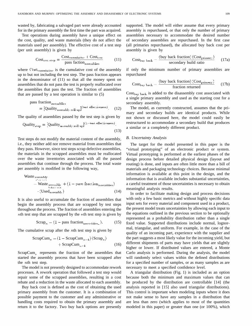
Fig. 4 illustrates the rough layout of the components usedin this analysis. Fig. 5 is a photograph of the interior of theactual FPD. Table II shows the list of components used in theFPD assembly, with the most likely values for the four basicinputs used.

The cost and composition (mass) of the components arelikely to be known at the time of purchase. However, there maystill be some fluctuation. These inputs were therefore enteredwith 10% triangular distributions. Although the analysisshown here lumps all materials together and gives a cumulativemass, in actual practice the amount of materials of interestwould be inventoried separately.


(a)

(b)

Fig. 2. Example user interface for entering inputs into the modeling tool. (a) Component input table. The buttons (labeled with “T” for triangulardistribution) are associated with the input field to their left. Pressing on these buttons provides the user with the option of including distributiondata.(b) Assembly process input table.

The quality of the component may or may not be known.Typically a minimum quality will be specified by the supplierand a most likely value can be estimated by the manufacturer

given any prior experience with the product. In this analysis,the values given in Table II are entered as the most likelyvalue (based on engineering knowledge for this general part


Fig. 3. Example results output interface for the modeling tool. Distributions may be plotted for any of the result fields.

Fig. 4. Schematic layout of flat panel display (FPD) components used inthis analysis.

type), with an upper bound of 100% and a lower bound thatmakes the distribution symmetric.

The waste generated in producing the product may or maynot be known; even if it is documented, the data may notbe made available from the supplier. Regardless, educatedguesses can typically be made for different product families(injection-molded plastic, PWB’s, IC’s, etc.). The accuracyof these values will depend upon the type of data generallyavailable and/or the ability to generate data using predictivemodels. For the analysis shown, the most likely value hasbeen entered based on the type and mass of component (orparts of the component) and the triangular distribution is setat 25%.

B. Primary Assembly Analysis

Consider only the primary assembly of the FPD first.Performing an analysis with the data described above (10 000samples evaluated) gives the results shown in Table III.

Table III shows that even when the values of waste forincoming components have up to a25% error, the finalresult has a relatively low error (10% at the 95% confidencelevel). This is partially due to the use of values for processwaste generation from within the company (i.e., during theassembly process) over which the manufacturer has controland for which there is high confidence data.

While Table III is a useful illustration of data confidence, themodel may also be used to optimize waste (or other metrics)when there are tradeoffs in selecting a particular component.For example, suppose a supplier offers a component with


Fig. 5. Photograph of the flat panel display.

TABLE IIINPUTS TO THE FPD ANALYSIS

TABLE IIIOUTPUTS THROUGH PRIMARY ASSEMBLY

lower incoming waste, but lower guaranteed quality. Since thelower quality will result in increased scrap, the designer mightwish to determine the amount of component waste reductionrequired to achieve an overall waste reduction for the product.An example of this type of tradeoff analysis for the backlight

assembly portion of the FPD is presented in Fig. 6. Averageincoming waste for the backlight assembly is plotted versusthe cumulative FPD waste for two different quality levels. Thegraph shows that incoming waste for the backlight assemblymust drop to less than 85% of the original backlight assembly


TABLE IVHIGH QUALITY VERSUS LOW COST ASSEMBLY COMPARISON

Fig. 6. Cumulative FPD waste versus the incoming waste for the backlightassembly for two different backlight assembly incoming qualities.

(assuming a 99% to 95% change in incoming quality) in orderto decrease the overall waste generation for the FPD.

The model may also be used exclusively within the designand manufacturing environment. An example of two differentassembly options is used to demonstrate this application.Assume that there are two assembly lines available. One costsan average of $1.50 per step (labor, equipment, and materials).The second costs an average of $3.00 per step but results in twoorders of magnitude increase in quality (i.e., 100 ppm defectsdrops to 1 ppm). As in the example given in material and com-ponent acquisition, only the primary assembly is considered.A comparison of the two assembly lines appears in Table IV.

In this case, three of the four metrics improved by going tothe higher quality assembly, primarily because of decreasedscrap. The outgoing quality increases slightly and the numberof units that must begin production decreases by more than5%. Although assembly costs increase by $15, the final costof producing a flat panel decreases by $89. Total waste dropsby 2% (less scrap from test steps). The material consumed doesnot change because the same amount of material is present ina “passed” assembly in both cases.

C. Disassembly and Secondary Assembly Analysis

The end-of-life scenario modeled in this paper is a combina-tion of remanufacture and disposal that examines a secondary

build of the same FPD using components from the originalbuild. After the primary units are repurchased or otherwisereacquired by the OEM at some fraction of the originalcost (for this analysis assumed to be 5%), the product isdisassembled. Since these particular components are fairlysimply assembled with screws and clamps, the disassembly isassumed to be equally simple with an average cost of $1.50 percomponent and greater than 95% yields. It was also assumedthat the individual components were in good working orderat the time of return with 85% of the electronics functioningand 90% of the display components still usable. The ability toavoid using poor quality components in the secondary product,is reasonably good, with test efficiencies ranging from 80 to90%. The ratio of secondary to primary builds is 0.25.

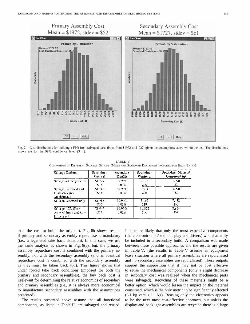
Given the assumptions above, the four basic metrics wereexamined for both the primary and secondary build. Thecost distributions at the 99% confidence level (3) indicatethat there is a clear economic advantage to using reclaimedcomponents. Assuming all the primary assemblies are repur-chased, the average cost drops from $1972 per unit to $1727per unit (Fig. 7), when buy back and disassembly costs areallocated to the secondary assemblies. The outgoing quality isapproximately unchanged at 99.95%. Total cumulative wasteis reduced from 12.7 to 2.2 kg and material consumed dropsfrom 9.0 to 1.1 kg. It can be seen from this example thathighly specific data and exact numbers may not be requiredfor basic business decisions. Given the above assumptions anddata distributions, it appears that salvage of components fromthis FPD is worth further consideration. In a real situation,finalization of the design and manufacturing strategy wouldrequire more detailed and specific data, but the initial analysis,gives the business unit reason to pursue a more detailed life-cycle assessment.

One of the advantages of the methodology presented inthis paper is the ability to perform sensitivity analyzes. Inorder to demonstrate this, the cost to build a flat paneldisplay from salvaged parts is plotted against the buy-back cost[Fig. 8(a)]. Error bars (1 ) are also plotted. The results showthat if buy back costs exceed 8% of the primary assemblycost (and all primary assemblies are repurchased), that asecondary assembly using salvaged parts is not economical.The economics of secondary assembly are considerably betterif only enough primary assemblies are repurchased to satisfythe secondary assembly requirements (even with 20% buy-back costs, the cost to build a refurbished FPD may be lower


Fig. 7. Cost distributions for building a FPD from salvaged parts drops from $1972 to $1727, given the assumptions stated within the text. The distributionsshown are for the 99% confidence level (3�).

TABLE VCOMPARISON OF DIFFERENT SALVAGE OPTIONS (MEAN AND STANDARD DEVIATIONS INCLUDED FOR EACH ENTRY)

than the cost to build the original). Fig. 8b shows resultsif primary and secondary assembly repurchase is mandatory(i.e., a legislated take back situation). In this case, we usethe same analysis as shown in Fig. 8(a), but, the primaryassembly repurchase cost is combined with the primary as-sembly, not with the secondary assembly (and an identicalrepurchase cost is combined with the secondary assemblyas they must be taken back too). This figure shows thatunder forced take back conditions (imposed for both theprimary and secondary assemblies), the buy back cost isirrelevant for determining the relative economics of secondaryand primary assemblies (i.e., it is always more economicalto manufacture secondary assemblies with the assumptionspresented).

The results presented above assume that all functionalcomponents, as listed in Table II, are salvaged and reused.

It is more likely that only the most expensive components(the electronics and/or the display and drivers) would actuallybe included in a secondary build. A comparison was madebetween these possible approaches and the results are givenin Table V; (the results in Table V assume an equipmentlease situation where all primary assemblies are repurchasedand no secondary assemblies are repurchased). These outputssupport the supposition that it may not be cost effectiveto reuse the mechanical components (only a slight decreasein secondary cost was realized when the mechanical partswere salvaged). Recycling of these materials might be abetter option, which would lessen the impact on the materialconsumed, which is the only metric to be significantly affected(3.1 kg versus 1.1 kg). Reusing only the electronics appearsto be the next most cost-effective approach, but unless thedisplay and backlight assemblies are recycled there is a large


(a)

(b)

Fig. 8. Secondary assembly cost of the FPD versus the primary assemblybuy back cost. Error bars represent 1�. (a) primary assembly repurchase isoptional, (b) primary and secondary assembly repurchase is mandatory.

negative impact in the amount of materials consumed (7.4 kg).A final decision on the best strategy requires a more detailedanalysis, but this high level assessment highlights the areas ofconcern and indicates where more detailed data and processinformation are required.

IV. CONCLUSION

The approach presented in this paper is not intended to beas accurate as a full and detailed life-cycle assessment andshould not be interpreted as a replacement for such. However,it does demonstrate the “80/20 rule,” which says that 80%accuracy can be obtained with 20% of the effort and data. It is

also a means of introducing nonenvironmental experts, such asthose in the design and business community, to the inclusion ofenvironmental merit into their decision making process. Thismethodology can be used to make high-level decisions andillustrates the point that a full life-cycle assessment is notnecessarily needed for every product, nor does the productneed to be defined in final detail.

Cost is typically one of the best known or most easilyestimated metrics. Unfortunately it is often not included in life-cycle assessments or DFE. Any uncertainty in the data inputsand corresponding error in the estimation can be captured byusing Monte Carlo simulation. As seen in the example of theprimary and secondary flat panel display builds, even witha 10% error for all inputs, the final error (at 2 or 95%confidence) is only $105 out of $1973 or 5% for the primarybuild and $124 out of $1727 or 7% for the secondary build.This metric is absolutely critical in the implementation of DFEinto the business environment. As pointed out in [15], MonteCarlo analysis is not intended to model partial information orhigher-order uncertainty, and therefore, does not take the placeof critical model inputs that may not be known. However,the use of Monte Carlo analysis allows the analyst to bracketand understand the error and potential risk associated with nothaving detailed data.

Minimum quality of incoming parts is typically specifiedby the supplier and maximum quality is theoretically always100%. In order to use a triangular distribution and MonteCarlo simulation to account for error, the user needs only toestimate the most likely value for the quality of an incomingcomponent or material. The quality of a process step must becalculated by combining the amount of production scrap foreach component with the number of field failures. These twoquantities can then be used to estimate test effectiveness. Inthe present analysis, test effectiveness is entered in order topredict scrap and field failures. The quality metric is expectedto be most useful when making comparisons and tradeoffs, asin the assembly example. In these cases, relative values areoften as valuable as absolute values for decision making.

If sales of the product occur over a significant periodof time (i.e., many months or years), then “time value ofmoney” may be a relevant contributor to life cycle costs intradeoff analyzes that consider product take back. Consider thefollowing simple example: an OEM must either purchase allthe parts to satisfy the entire production run for a product up-front before production begins, or gradually over time duringproduction. In the up-front purchase case, the real cost to theOEM of the parts is the amount paid for the parts plus the“opportunity cost” associated with the up-front payment, i.e.,the money to make the up-front payment was either borrowedat some interest rate and can not be repaid until the productsare sold, or equivalently, the money for the up-front paymentis wrapped up in products yet to be sold instead of in the bankearning interest. Whether interest is paid or interest is lost,the opportunity cost must be considered when computing thelife cycle cost of the product. In the second case, the OEMmay have to contend with inflation that increases the part costover time. In both cases, remanufacturing leads to additionalpotential savings because it requires the purchase of a smaller


inventory of parts, thus tying up less money in unsold productsand/or creating less exposure to inflation effects. To properlytreat the time value of money, a production/inventory model(e.g., [10] or [11]) that includes production volumes, anddetailed time lines for primary and secondary manufacturingand product is necessary. This is an analysis which is outsidethe scope of the model presented here.

Waste is typically the least characterized of the metricspresented in the model. For the purpose of demonstratingthe methodology, all waste was lumped together. In an actualproduct design, it would be desirable to categorize the differenttypes of waste, such as by disposal method. The amountof waste generated per product may often be inaccurate andpotentially underestimated because it is common to combinewaste for the entire facility. The analysis in this paper madehigh level assumptions about the amount of waste producedin manufacturing components of certain types. Developmentof more detailed data modules and/or predictive modules forelectronic components will be critical for correctly accountingfor this metric.

Material use is of most interest when the inventory resultsare incorporated into an impact analysis. In this paper, thematerial use metric was kept very simple. As in the case ofwaste, more module and model development for electronicproducts is needed. However, as in the case of waste, theremay be many high level decisions that can be made by simplytracking a small number of materials of interest or concern.

ACKNOWLEDGMENT

The authors wish to thank C. Mizuki, G. Pitts, and P.Gilchrist, MCC, P. Spletter, Nu Thena Systems, and J. Smith,Battelle, for their useful discussions and contributions associ-ated with this work, and the MCC Low Cost Portables Projectfor providing the details of the flat panel display used for theexample analysis in this paper.

REFERENCES

[1] J. A. Stuart, M. K. Low, D. J. Williams, L. J. Turbini, and J. C.Ammons, “Challenges in determining electronics equipment take-backlevels,” IEEE Trans. Comp., Packag., Manufact. Technol. C, vol. 21, pp.225–232, July 1998.

[2] V. Berko-Boateng, J. Azar, E. De Jong, and G. A. Yander, “Asset recyclemanagement—A total approach to product design for the environment,”in Proc. IEEE Int. Symp. Electron. Environ., 1993, pp. 138–144.

[3] J. A. Stuart, L. J. Turbini, and J. C. Chumley, “Investigation of electronicassembly design alternatives through production modeling of life cycleimpacts, costs, and yield,”IEEE Trans. Comp., Packag., Manufact.Technol. C, vol. 20, pp. 317–326, Oct. 1997.

[4] T. A. Hanft and E. Kroll, “Ease-of-disassembly evaluation in design forrecycling,” in Design for X: Concurrent Engineering Imperatives, G. Q.Huang, Ed. London, U.K.: Chapman & Hall, 1996.

[5] R. L. Tummala and B. E. Koenig, “Models for life cycle assessmentof manufactured products,” inProc. IEEE Int. Symp. Electron. Environ.,1994, pp. 94–99.

[6] R. W. Chen, D. Navin-Chandra, and F. B. Prinz, “Cost-benefit analysismodel of product design for recyclability and its application,”IEEETrans. Comp., Packag., Manufact. Technol. A, vol. 17, pp. 502–507,Dec. 1994.

[7] B. A. Bras and J. Emblemevag, “Activity-based costing and uncertaintyin designing for the life-cycle,” inDesign for X: Concurrent EngineeringImperatives, G. Huang, Ed. London, U.K.: Chapmann & Hall, 1996.

[8] M. Simon, “Objective assessment of designs for recycling,” inProc. 9thInt. Conf. Eng. Design, vol. 2, pp. 832–835, 1993.

[9] M. K. Low, D. J. Williams, and C. Dixon, “Manufacturing productswith end-of-life considerations: An economic assessment to the routes ofrevenue generation from mature products,”IEEE Trans. Comp., Packag.,Manufact. Technol. C, vol. 21, pp. 4–10, Jan. 1998.

[10] D. P. Heyman, “Optimal disposal policies for a single-item inventorysystem with returns,”Naval Res. Logist. Quart., vol. 24, pp. 385–405,Feb. 1977.

[11] E. van der Laan and M. Solomon, “Production planning and inventorycontrol with remanufacturing and disposal,”Eur. J. Oper. Res., vol.102, pp. 264–278, 1997.

[12] P. A. Sandborn and M. Vertal, “Analyzing packaging trade-offs dur-ing system design,”IEEE Design Test Comput., vol. 15, pp. 10–19,July–Sept. 1998.

[13] T. W. Williams and N. C. Brown, “Defect level as a function of faultcoverage,”IEEE Trans. Comput., vol. C-30, pp. 987–988, Dec. 1981.

[14] C. F. Murphy, M. Abadir, and P. Sandborn, “Economic analysis oftest and known good die or multichip assemblies,”J. Electron. Testing(JETTA), pp. 151–166, 1997.

[15] E. Regnier and W. F. Hoffman III, “Uncertainty model for productenvironmental performance sorting,” inProc. IEEE Int. Symp. Electron.Environ., 1998, pp. 207–212.

[16] E. Zussman, A. Kriwet, and G. Seliger, “Disassembly-oriented assess-ment methodology to support design for recycling,”Annals Int. Inst.Prod. Eng. Res., vol. 43, no. 1, pp. 9–14, 1994.

[17] R. Nolan, “MCC low cost portables report: MCC-DTA-025-96 (P),”Microelectron. Comput. Technol. Corp., 1996.

[18] C. F. Murphy, C. Mizuki, and P. A. Sandborn, “Implementation ofDFE in the electronics industry using simple metrics for cost, quality,and environmental merit,” inProc. IEEE Int. Symp. Electron. Environ.,1998, pp. 219–224.

Peter A. Sandborn (M’87) received the B.S. degree in engineering physicsfrom the University of Colorado, Boulder, in 1982, and the M.S. degree inelectrical science and the Ph.D. degree in electrical engineering, both fromthe University of Michigan, Ann Arbor, in 1983 and 1987, respectively.

He is an Associate Professor in the CALCE Electronic Products andSystems Center (EPSC), University of Maryland, College Park, where hisinterests include technology tradeoff analysis for electronic packaging, systemlife cycle and risk economics, hardware/software codesign, and design tooldevelopment. Prior to joining the University of Maryland, he was a founderand Chief Technical Officer of Savantage, Austin, TX, and a Senior Memberof Technical Staff at the Microelectronics and Computer Technology Corpora-tion, Austin. He is the author of over 50 technical publications and one bookon multichip module design.

Dr. Sandborn is an Associate Editor of the IEEE TRANSACTIONS ON

ELECTRONICS PACKAGING MANUFACTURING.

Cynthia F. Murphy received the B.S. degree in geology from the College ofWilliam and Mary, Williamsburg, VA and the M.S. degree in geology fromthe University of North Carolina, Chapel Hill.

She is a Senior Member of Technical Staff and a Project Managerwith the Environmental Programs Division, Microelectronics and ComputerTechnology Corporation (MCC), Austin TX. During her 11 years at MCC,she has worked in the areas of environmentally conscious manufacture ofelectronics and in a variety of technologies related to the manufacture of highperformance electronics. Much of her focus has been on the economic analysisof electronics systems and she has authored and co-authored numerous papersin this area. In addition, she has worked in reliability and process assessmentof multichip modules and their components. Prior to joining MCC, she wasemployed by Motorola in the Semiconductor Products Sector. She spent fouryears working as a Process Engineer and then as a Product Engineer. Inboth job functions her primary responsibilities centered on data collection andstatistical analysis.

Documents

A model for optimizing the assembly and disassembly of electronic