A model for a time and frequency Granger causality measure

A model for a time and frequency Granger causalitymeasure for intracranial electroencephalogram data

Olivier Renaud

Joint work with Sezen Cekic and Didier Grandjean

http://www.unige.ch/fapse/mad – Dept. of Psychology – University of Geneva

MathStatNeuro workshop, Nice, September 2015

O. Renaud Nice 2015 Time-Frequency Granger Causality 1

http://www.unige.ch/fapse/mad

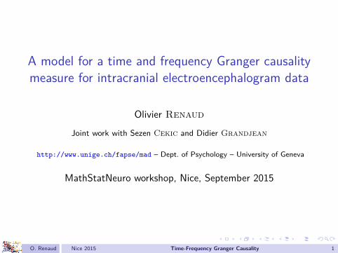
All others must bring data

0 200 400 600 800 1000 1200−200

−100

0

100

200

0 200 400 600 800 1000 1200−300

−200

−100

0

100

200

300


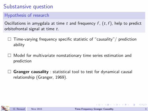
Substansive questionHypothesis of researchOscillations in amygdala at time t and frequency f , (t, f ), help to predictorbitofrontal signal at time t.

Time-varying frequency specific statistic of “causality”/ predictionability

Model for multivariate nonstationary time series estimation andprediction

Granger causality : statistical tool to test for dynamical causalrelationship (Granger, 1969).


Granger causalityAxiomatic impositionCause necessarily precedes its effect in time.

DefinitionIf a signal X “Granger-causes” another signal Y , then past values of Xshould contain information that helps to predict Y above and beyond theinformation contained in past values of Y alone ((Granger, 1969)).

→ Causality in the Wiener-Granger sense is based on the statisticalpredictability of one time series based on knowledge of one other.

• Simple and interpretable method• Can it be time and frequency specific ?


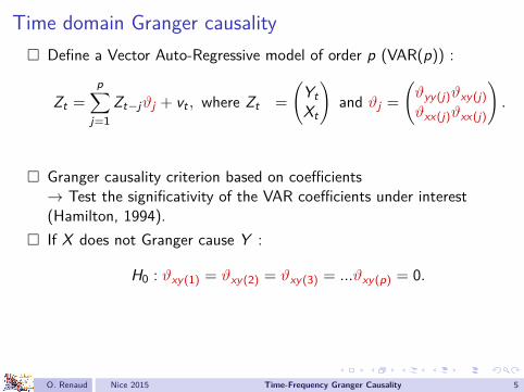
Time domain Granger causality Define a Vector Auto-Regressive model of order p (VAR(p)) :

Zt =p∑

j=1Zt−jϑj + vt , where Zt =

(YtXt

)and ϑj =

(ϑyy(j)ϑxy(j)ϑxx(j)ϑxx(j)

).

Granger causality criterion based on coefficients→ Test the significativity of the VAR coefficients under interest(Hamilton, 1994).

If X does not Granger cause Y :

H0 : ϑxy(1) = ϑxy(2) = ϑxy(3) = ...ϑxy(p) = 0.


Frequency domain Granger causality Spectral decomposition of the time domain statistics by Fourier

transform of the VAR model (Geweke, 1982, 1984).• Geweke-Granger causality statistic (Geweke, 1984)

• Partial Directed Coherence (Baccalà and Sameshima, 2001)

• Directed Transfer Function (Kaminski and Blinowska, 1991)


Time-varying Granger causality Neuroscience data : intrinsically nonstationary→ Characteristic of interest !→ Statistic of causality that catches the dynamic of the causalitypattern through time

Practically → the density pt(Zt |Z t−pt−1 ) different for each time.

→ VAR model that evolves in time.

Two widely used approaches to estimate a time varying VAR model

• Windowing approach - assumes locally stationarity• Adaptive estimation approach - assumes slowly varying

parameters


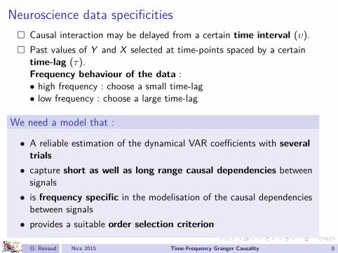
Neuroscience data specificities Causal interaction may be delayed from a certain time interval (υ). Past values of Y and X selected at time-points spaced by a certain

time-lag (τ).Frequency behaviour of the data :• high frequency : choose a small time-lag• low frequency : choose a large time-lag

We need a model that :

• A reliable estimation of the dynamical VAR coefficients with severaltrials• capture short as well as long range causal dependencies between

signals• is frequency specific in the modelisation of the causal dependencies

between signals• provides a suitable order selection criterion


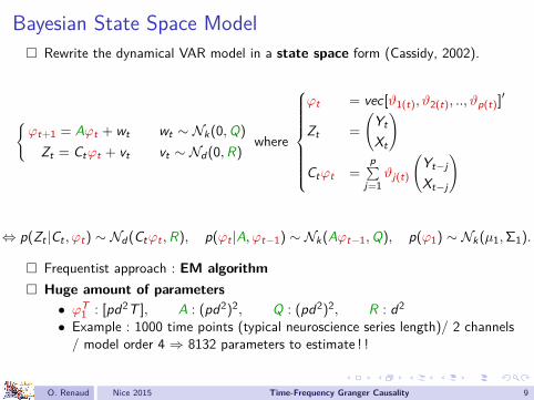
Bayesian State Space Model Rewrite the dynamical VAR model in a state space form (Cassidy, 2002).

ϕt+1 = Aϕt + wt wt ∼ Nk(0,Q)

Zt = Ctϕt + vt vt ∼ Nd (0,R)where

ϕt = vec[ϑ1(t), ϑ2(t), .., ϑp(t)]′

Zt =(

Yt

Xt

)

Ctϕt =p∑

j=1ϑj(t)

(Yt−j

Xt−j

)

⇔ p(Zt |Ct , ϕt) ∼ Nd (Ctϕt ,R), p(ϕt |A, ϕt−1) ∼ Nk(Aϕt−1,Q), p(ϕ1) ∼ Nk(µ1,Σ1).

Frequentist approach : EM algorithm Huge amount of parameters

• ϕT1 : [pd2T ], A : (pd2)2, Q : (pd2)2, R : d2

• Example : 1000 time points (typical neuroscience series length)/ 2 channels/ model order 4 ⇒ 8132 parameters to estimate ! !


Variational Bayes Bayesian approach → Ωb

1 = A,Q,R random Target quantity : posterior distribution p(ϕT

1 ,Ωb1 |ZT

1 )→ Intractable integral of very high dimension

Variational approximationPosterior density p(ϕT

1 ,Ωb1 |ZT

1 ) → approximated by a variational posteriordensity

p(ϕT1 ,Ωb

1 |ZT1 ) ≈ q(ϕT

1 ,Ωb1 |ZT

1 ).

Find the distribution q(ϕT1 ,Ωb

1 |ZT1 ) that minimizes the KL-divergence

between p(ϕT1 ,Ωb

1 |ZT1 ) and q(ϕT

1 ,Ωb1 |ZT

1 )

KL(q(ϕT

1 ,Ωb1 |ZT

1 )‖p(ϕT1 ,Ωb

1 |ZT1 ))

=⟨log q(ϕT

1 ,Ωb1 |ZT

1 )p(ϕT

1 ,Ωb1 |ZT

1 )

⟩q(ϕT

1 ,Ωb1 |ZT

1 )

〈.〉 : expectation, subscript : density used for this expectation.


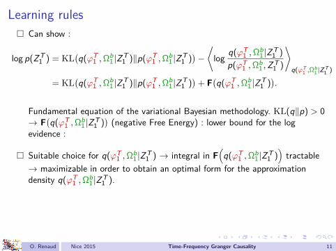
Learning rules Can show :

log p(ZT1 ) = KL

(q(ϕT

1 ,Ωb1 |ZT

1 )‖p(ϕT1 ,Ωb

1 |ZT1 ))−⟨log q(ϕT

1 ,Ωb1 |ZT

1 )p(ϕT

1 ,Ωb1 ,ZT

1 )

⟩q(ϕT

1 ,Ωb1 |ZT

1 )

= KL(q(ϕT

1 ,Ωb1 |ZT

1 )‖p(ϕT1 ,Ωb

1 |ZT1 ))

+ F(q(ϕT

1 ,Ωb1 |ZT

1 )).

Fundamental equation of the variational Bayesian methodology. KL(q‖p) > 0→ F

(q(ϕT

1 ,Ωb1 |ZT

1 ))(negative Free Energy) : lower bound for the log

evidence :

Suitable choice for q(ϕT1 ,Ωb

1 |ZT1 ) → integral in F

(q(ϕT

1 ,Ωb1 |ZT

1 ))tractable

→ maximizable in order to obtain an optimal form for the approximationdensity q(ϕT

1 ,Ωb1 |ZT

1 ).


Mean-field approximation Assumption underlying the variational Bayes methodology :

q(ϕT1 ,Ωb

1 |ZT1 ) = q(ϕT

1 |ZT1 )

b∏j=1

q(Ωj |ZT1 ).

Free energy (model evidence lower bound) can be rewritten

F(q(ϕT

1 |ZT1 ), q(Ω1|ZT

1 ), . . . , q(Ωb|ZT1 )).

→ Mean field approximation may have minor to major impacts on theresulting inference depending on the model at hand


Variational EM algorithm Maximizing the functional F

(q(ϕT

1 |ZT1 ), q(Ω1|ZT

1 ), . . . , q(Ωb|ZT1 ))

(calculus of variations)→ Iterative optimal forms for q(ϕT

1 |ZT1 ), q(Ω1|ZT

1 ), . . . , q(Ωb|ZT1 ).

q∗(ϕT1 |ZT

1 )(l+1) ∝ exp⟨log p(ϕT

1 |Ωb1 ,ZT

1 )⟩(l)

q(Ωb1 |ZT

1 ),

q∗(Ωm|ZT1 )(l+1) ∝ exp

⟨log p(Ωb

1 |ϕT1 ,ZT

1 )⟩(l)

−Ωm,

where 〈.〉(l)−Ωmis the expectation over all the distributions at iteration (l)

except q(Ωm|ZT1 )(l) (Beal, 2003; Ostwald et al., 2014).

TheoremIf the complete-data likelihood p(ϕT

1 ,ZT1 |Ωb

1) is part of the exponential family[...] and if the hidden and parameter priors distributions p(ϕT

1 ) and p(Ωb1) are

conjugate to this complete-data likelihood, the corresponding variationalapproximate posterior distributions that maximize F, q∗(ϕT

1 |ZT1 ) and q∗(Ωb

1 |ZT1 ),

are of the same distributional form than respectively the prior distributions p(ϕT1 )

and p(Ωb1).


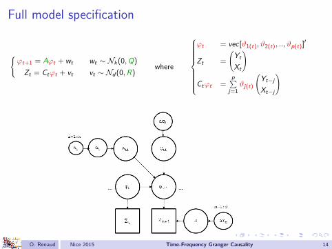
Full model specification

ϕt+1 = Aϕt + wt wt ∼ Nk(0,Q)

Zt = Ctϕt + vt vt ∼ Nd (0,R)where

ϕt = vec[ϑ1(t), ϑ2(t), .., ϑp(t)]′

Zt =(

Yt

Xt

)

Ctϕt =p∑

j=1ϑj(t)

(Yt−j

Xt−j

)


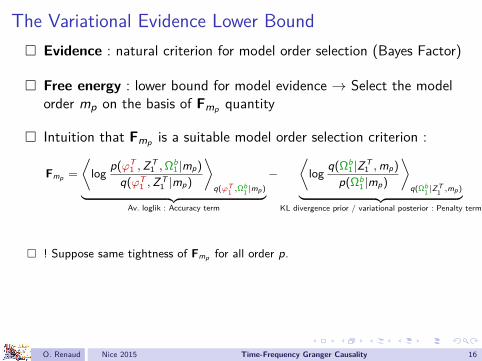
The Variational Evidence Lower Bound Evidence : natural criterion for model order selection (Bayes Factor)

Free energy : lower bound for model evidence → Select the modelorder mp on the basis of Fmp quantity

Intuition that Fmp is a suitable model order selection criterion :

Fmp =⟨

log p(ϕT1 , Z T

1 , Ωb1 |mp)

q(ϕT1 , Z T

1 |mp)

⟩q(ϕT

1 ,Ωb1 |mp)︸︷︷︸

Av. loglik : Accuracy term

−⟨

log q(Ωb1 |Z T

1 , mp)p(Ωb

1 |mp)

⟩q(Ωb

1 |ZT1 ,mp)︸︷︷︸

KL divergence prior / variational posterior : Penalty term

! Suppose same tightness of Fmp for all order p.


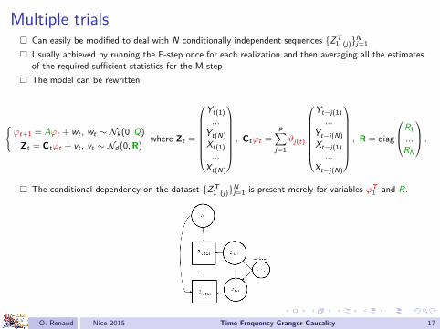
Multiple trials Can easily be modified to deal with N conditionally independent sequences ZT

1 (j)Nj=1 Usually achieved by running the E-step once for each realization and then averaging all the estimates

of the required sufficient statistics for the M-step The model can be rewritten

ϕt+1 = Aϕt + wt , wt ∼ Nk(0,Q)Zt = Ctϕt + vt , vt ∼ Nd (0,R)

where Zt =

Yt(1)...

Yt(N)Xt(1)...

Xt(N)

, Ctϕt =

p∑j=1

ϑj(t)

Yt−j(1)...

Yt−j(N)Xt−j(1)...

Xt−j(N)

, R = diag

R1...RN

.

The conditional dependency on the dataset ZT1 (j)Nj=1 is present merely for variables ϕT

1 and R.


Bayesian State Space Multiscale ModelWe have A reliable estimation of the dynamical VAR coefficients in a several

trials situation A suitable model order selection criterion

We need to capture short- and long-range causal dependencies between signals

(better than υ and τ parameters) to be frequency specific in the modelisation of the causal

dependencies between signals

⇒ Bayesian State Space Multiscale Model


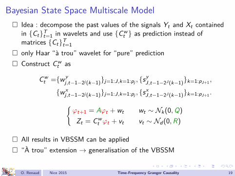
Bayesian State Space Multiscale Model Idea : decompose the past values of the signals Yt and Xt contained

in CtTt=1 in wavelets and use Cwt as prediction instead of

matrices CtTt=1 only Haar “à trou” wavelet for “pure” prediction Construct Cw

t as

Cwt =wy

j,t−1−2j (k−1)j=1:J,k=1:pj , syJ,t−1−2J (k−1)k=1:pJ+1 ,

wxj,t−1−2j (k−1)j=1:J,k=1:pj , sx

J,t−1−2J (k−1)k=1:pJ+1 .ϕt+1 = Aϕt + wt wt ∼ Nk(0,Q)Zt = Cw

t ϕt + vt vt ∼ Nd (0,R)

All results in VBSSM can be applied “À trou” extension → generalisation of the VBSSM


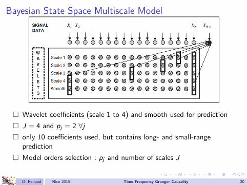
Bayesian State Space Multiscale Model

Wavelet coefficients (scale 1 to 4) and smooth used for prediction J = 4 and pj = 2 ∀j only 10 coefficients used, but contains long- and small-range

prediction Model orders selection : pj and number of scales J


Bayesian State Space Multiscale ModelMultiresolution methodology benefits :

• Wavelets coefficients wj directly related to a specific frequency band→ frequency specific in the modelisation of the causal relationship• Capture short and long-range dependencies between signals with

only few parameters→ Avoids the choice of the time interval (υ) time-lag τ• Simple and suitably interpretable time-varying Granger causalitystatistic (Chicharro, 2011)


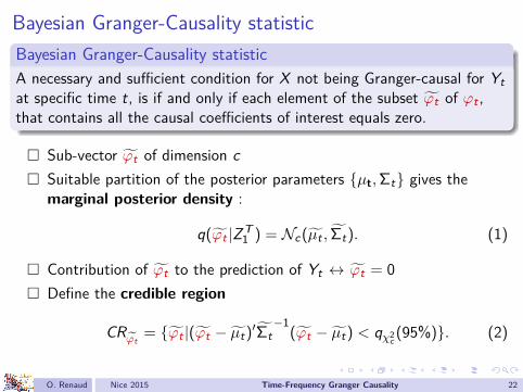
Bayesian Granger-Causality statisticBayesian Granger-Causality statisticA necessary and sufficient condition for X not being Granger-causal for Ytat specific time t, is if and only if each element of the subset ϕt of ϕt ,that contains all the causal coefficients of interest equals zero.

Sub-vector ϕt of dimension c Suitable partition of the posterior parameters µt,Σt gives the

marginal posterior density :

q(ϕt |ZT1 ) = Nc(µt , Σt). (1)

Contribution of ϕt to the prediction of Yt ↔ ϕt = 0 Define the credible region

CRϕt= ϕt |(ϕt − µt)′Σt

−1(ϕt − µt) < qχ2c (95%). (2)


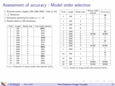
Assessment of accuracy : Model order selection Bivariate system, lengths 500; 1000; 2000, Trials 1; 10 ϕT

1 Markovian Estimation performed for orders p = 1 : 10 Results based on 100 simulations

Trials Length Model order True model selected1 500 1 83%1 500 2 95%1 500 4 96%1 500 8 97%1 1000 1 87%1 1000 2 100%1 1000 4 97%1 1000 8 99%1 2000 1 89%1 2000 2 99%1 2000 4 100%1 2000 8 98%10 500 1 89%10 500 2 98%10 500 4 100%10 500 8 100%

Table: Proportion of correct model order selection by Fmp

Trials Length Model order Wrong model Occurrenceselected

1 500 1 2 163 1

1 500 2 3 34 2

1 500 4 5 4

1 500 8 5 26 1

1 1000 1 2 131 1000 2 NONE NONE1 1000 4 5 31 1000 8 6 11 2000 1 2 111 2000 2 3 11 2000 4 NONE NONE

1 2000 8 4 17 1

10 500 1 2 83 3

10 500 2 3 14 1

10 500 4 NONE NONE10 500 8 NONE NONE

Table: Details on wrong model order selections by Fmp .


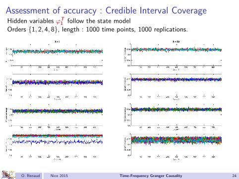
Assessment of accuracy : Credible Interval CoverageHidden variables ϕT

1 follow the state modelOrders 1, 2, 4, 8, length : 1000 time points, 1000 replications.


Assessment of accuracy : Credible Interval CoverageHidden variables ϕT

1 evolve slowly & deterministicallyOrders 1, 2, 4, 8, length : 1000 time points, 1000 replications.


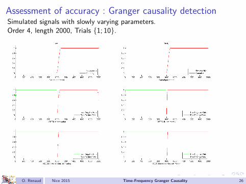
Assessment of accuracy : Granger causality detectionSimulated signals with slowly varying parameters.Order 4, length 2000, Trials 1; 10.


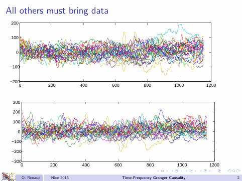
All others must bring data

0 200 400 600 800 1000 1200−200

−100

0

100

200

0 200 400 600 800 1000 1200−300

−200

−100

0

100

200

300


Application iEEG data recorded during psychological experimental situations in

four epileptic pharmaco-resistant patients

Recordings localized within the amygdala and medial orbito-frontalcortex

Study the dynamics of neuronal processes within and between theseregions in response to emotional prosody exposure (Christen andGrandjean, 2010)

Two experimental conditions : anger and neutral

A significant Granger causality from signal 1 to signal 2 at frequency f andat time t means that the energy of signal 1 at frequency f significantlyimproves the prediction of the value of signal 2 at time t.


ApplicationP-values in log10 scale for the overall causality statistic and for each scale.For anger and neutral.


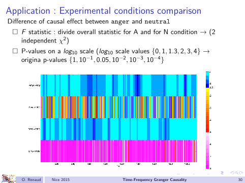
Application : Experimental conditions comparisonDifference of causal effect between anger and neutral

F statistic : divide overall statistic for A and for N condition → (2independent χ2)

P-values on a log10 scale (log10 scale values 0, 1, 1.3, 2, 3, 4 →origina p-values 1, 10−1, 0.05, 10−2, 10−3, 10−4


Application : Discussion Multiple testing : the frequency dimension

• → Hierarchically testing• → usually relaxed in Neuroscience (GCC, PDC, DTF)

Multiple testing : the time dimension

• Threshold : α level but take into account periods of significanceonly if they are sustained enough

• Bonferroni correction (too conservative)• Cluster mass test (Maris and Oostenveld, 2007)


ReferencesBaccalà, L. A. and K. Sameshima (2001). Partial directed coherence : a new concept in neural structure determination. Biological cybernetics 84(6), 463–474.Beal, M. (2003). Variational Algorithms for Approximate Bayesian Inference. Ph. D. thesis, University College London, London.Cassidy, M.J. Penny, W. (2002). Bayesian nonstationary autoregressive models for biomedical signal analysis. Biomedical Engineering, IEEE Transactions on 49(10), 1142–1152.Cekic, S. (2010). Lien entre activité neuronale des sites cérébraux de l’amygdale et du cortex orbito-frontal en réponse à une prosodie émotionnelle : investigation par la Granger-causalité.

Master Thesis, Université de Genève.Chicharro, D. (2011). On the spectral formulation of granger causality. Biological cybernetics 105(5-6), 331–347.Christen, A. and D. Grandjean (2010). Temporal dynamics of amygdala and orbitofrontal responses to emotional prosody using intracerebral local field potentials in humans. In Speech

Prosody, Volume 100874, Chicago, pp. 1–4.Ding, M., S. L. Bressler, W. Yang, and H. Liang (2000). Short-window spectral analysis of cortical event-related potentials by adaptive multivariate autoregressive modeling : data

preprocessing, model validation, and variability assessment. Biological cybernetics 83(1), 35–45.Geweke, J. (1982). Measurement of Linear Dependence and Feedback Between Multiple Time Series. Journal of the American Statistical Association 77(378), 304–313.Geweke, J. F. (1984). Measures of Conditional Linear Dependence and Feedback Between Time Series. Journal of the American Statistical Association 79(388), 907–915.Granger, C. W. J. (1969). Investigating Causal Relations by Econometric Models and Cross-spectral Methods. Econometrica 37(3), 424–438.Hamilton, J. D. (1994). Time series analysis, Volume 2. Princeton university press Princeton.Huang, A., M. P. Wand, et al. (2013). Simple marginally noninformative prior distributions for covariance matrices. Bayesian Analysis 8(2), 439–452.Kaminski, M. and K. Blinowska (1991). A new method of the description of the information flow in the brain structures. Biological cybernetics 65(3), 203–210.Maris, E. and R. Oostenveld (2007). Nonparametric statistical testing of eeg-and meg-data. Journal of neuroscience methods 164(1), 177–190.Menictas, M. and M. P. Wand (2013). Variational inference for marginal longitudinal semiparametric regression. Stat 2(1), 61–71.Ostwald, D., E. Kirilina, L. Starke, and F. Blankenburg (2014). A tutorial on variational bayes for latent linear stochastic time-series models. Journal of Mathematical Psychology 60, 1–19.Renaud, O., J.-L. Starck, and F. Murtagh (2003). Prediction based on a multiscale decomposition. International Journal of Wavelets, Multiresolution and Information Processing 1(2),

217–232.Schlögl, A. (2000). The electroencephalogram and the adapdative autoregressive model : theory and applications. Ph. D. thesis, University of Graz, Graz.Schlögl, A., S. Roberts, and G. Pfurtscheller (2000). A criterion for adaptive autoregressive models. In Proceedings of the 22 nd IEEE International Conference on Engineering in Medicine

and Biology, pp. 1581–1582.


Documents

A model for a time and frequency Granger causality measure