Embed Size (px)
Citation preview
A Model-Based Process for Evaluating Cluster
Building Blocks
Laura Keys
Electrical Engineering and Computer SciencesUniversity of California at Berkeley
Technical Report No. UCB/EECS-2010-117
http://www.eecs.berkeley.edu/Pubs/TechRpts/2010/EECS-2010-117.html
August 18, 2010

Copyright © 2010, by the author(s).All rights reserved.
Permission to make digital or hard copies of all or part of this work forpersonal or classroom use is granted without fee provided that copies arenot made or distributed for profit or commercial advantage and that copiesbear this notice and the full citation on the first page. To copy otherwise, torepublish, to post on servers or to redistribute to lists, requires prior specificpermission.
Acknowledgement
Thanks to Randy H. Katz for direction and guidance on this project and toDavid Culler for his valuable input. Many thanks to the indispensible AlbertGoto and Jon Kuroda for their fast, effective help in getting systems up andkeeping them running, Stephen Dawson-Haggerty for his help in dealingwith various power meters, Yanpei Chen for initially laying the groundworkfor investigating power-efficiency in Hadoop, John Davis and SuzanneRivoire for their part in the initial cluster comparison and modeling work,Ken Lutz and the SIGCluster group for their efforts in creating an energy-proportional cluster on which to conduct research, and all the LoCal-ersand affiliates who gave feedback and encouragement along the way. Thiswork was made possible by a fellowship from NDSEG.
A Model-Based Process for Evaluating
Cluster Building Blocks
Laura Keys
August 18, 2010
Abstract
Traditional servers account for more than 1.5% of the US electricity use though
spend their lives largely underutilized or idle. Because a large portion of power in
a data center is due directly or indirectly to servers, power savings in a data center
environment can be achieved simply by using lower power hardware in place of these
traditional servers. However, deciding which hardware to use in place of servers is
complicated because lower power typically equates to lower performance and because
different cluster owners use different metrics of success in quantifying cluster perfor-
mance. In this project report I present measurements from several single-machine
and system benchmarks for both interactive and batch jobs and develop predictive
models for power and performance within a cluster. Accurately predicting power to
within 10% based on OS-reported metrics requires similar training and testing bench-
marks, while predicting performance within a heterogeneous web server is simple and
straightforward. I also introduce a Cluster Visualizer for comparing potential cluster
configurations based on the actual benchmark measurements and different metrics of
value, ultimately making the decision about which hardware platform to build a cluster
from less complicated.
1 Introduction
Organizations ranging from Google to university research groups to the Federal government
have come to rely on data centers for their service hosting needs. In total these US data
centers consumed 61 billion KWh in 2006, more than the electricity consumed by all the
color televisions in the US during the same period, with an expected doubling of energy
usage by 2011 [18]. While HVAC, lighting, and other infrastructure are responsible for a
1

portion of this energy usage, as encompassed by the PUE (Power Usage Effectiveness) met-
ric, servers themselves consume an ever-increasing amount of energy per year, accounting
for 1.5% of national electricity use within the US as of 2007. To reduce server energy usage
by up to 80%, the EPA suggests some “best practices” and “state-of-the-art” solutions that
include adopting “energy-efficient” servers (servers that attain high performance per ex-
pended energy), employing aggressive server and storage consolidation, and enabling power
management within the data center down to the application level [18].
Aggressive power management within servers is a promising direction because, despite
their high energy usage, servers tend to operate at low utilizations. A survey from Google
showed that most servers tend to spend their time being utilized between 30 to 50% [2].
While this low level of utilization is reasonable in order to attain good performance and
response times, these servers generally draw a disproportionately large amount of energy
for such low utilization. In energy-proportional machines, in which power consumption
corresponds directly to resource consumption, we would expect these machines to use 30 to
50% of their maximum power. However, we do not see this being the case in server-class
machines today, with idle high-performance servers typically drawing upwards of 50 to 70%
of their maximum power.
Power consumption varies between different classes of machines; traditionally, embedded
systems have always considered power as a first-class constraint because they have an energy
supply limited by battery capacity, so they exhibit low idle power when not in use, whereas
servers have only recently started to take power into consideration. Many servers may have
been designed to support various low-power S-states between “on” and “off” but cannot
actually take advantage of these low power states due to a combination of board design and
operating system settings.
Thus, it appears that one could attain energy savings simply from switching to lower
power hardware, though this lower power often comes with a performance hit. System
designers, particularly at the server level, do not typically consider energy-savings as a first-
level constraint because it is a complicated matter, impacted by both hardware and software
use. The first complication is that power and energy are two different quantities, despite
their terms often being used interchangeably. Power is an instantaneous rate of electricity
consumption, typically reported in Watts or Kilowatts. Energy is the total amount of power
consumed integrated over some time period, reported in Joules or Kilowatt-hours. Thus,
a high-power server that consumes twice the power of a mobile node but completes a task
twice as fast will consume the same amount of energy for this task as the mobile node.
2
The second complication is that low power often equates to low performance in the
computing world. While a cluster composed entirely of small embedded processors would
have a very small power footprint, it would probably offer very low performance, a tradeoff
which is not in the best interests of a business that cannot afford to lose customers because
the company’s website took too long to load. Thus, traditional servers are the norm for a
company trying to err on the conservative side of offering too much performance. However,
there is now some interest in replacing traditional server nodes with high-performing low-
power nodes.
This project report makes the following contributions: it compares performance and
power-efficiency across a variety of workloads, including both interactive and batch jobs,
for three different computing platforms, presents linear models for predicting power and
performance within a real application, and introduces a GUI for comparing potential new
clusters. Section 2 discusses related work in building and modeling power-efficient clusters.
Section 3 presents three different types of hardware, four benchmarks, and the results of
running the benchmarks across single-node systems of each hardware type. Section 4 then
describes the two-step process for predictive power modeling and the results of this modeling
for single-machine systems of these hardware types. Section 5 also predicts performance for
a web server application. Section 6 discusess limitations and improvements for predictive
power modeling. Finally, Section 7 introduces a GUI for visualizing the tradeoffs between
power and performance of potential heterogeneous clusters composed of these underlying
hardware types.
2 Related Work
A power-efficient cluster is one that attains some high level of work per unit of power
consumed. The first step to building a power-efficient cluster is to select the most power-
efficient building blocks, though there has been much debate about what these building
blocks actually are. The authors of FAWN present a system composed of low-power, low-
performance nodes and advocate for building clusters out of so-called “wimpy” or embedded
nodes [1]. Interestingly, their design does not arise out of an attempt to obtain energy-
proportionality and power-efficiency but instead out of the desire to create a more balanced
system in which CPU speed can once again be matched by I/O capabilities. Lim et al.
use simulation to select the best out of six different systems according to the metric of
performance per dollar [14]. The cost part of this metric incorporates both up-front hardware
3
costs as well as longterm power and cooling costs. They also conjecture that higher powered
CPUs may be required for CPU- and I/O-intensive workloads that would otherwise saturate
CPU capacity in an embedded node. Keys et al. build and measure energy in homogeneous
clusters consisting of different classes of hardware and conclude that mobile nodes and high-
end servers provide the greatest power-efficiency [11]. They advocate that future clusters
be built out of high performing mobile nodes.
Blade servers such as CEMS, a blade-based design of dual core Athlon desktop-class
processors, have been proposed as a power-efficient cluster platform [6]. However, while
highly efficient in terms of power density, it is this same density that often requires blade
systems to have costly custom cooling solutions, as the rack power is higher than that in
traditional servers. Substituting embedded processors in place of these desktop machines
does not seem to be a silver bullet either. Reddi et al. demonstrate that embedded processors
targeting the web search application space jeopardize quality of service because they do
not have enough processing head room to absorb spikes in the workload without extensive
overprovisioning and underutilization, though they acknowledge that smaller cores lower the
total cost of ownership for a cluster [15].
A variant on the idea of power-efficiency is energy-proportionality. Barosso defines
energy-proportionality as energy consumption that is proportional to the usage of some
underlying resource. Thus, an energy-proportional cluster is one that uses an amount of
energy that is proportional to its compute resources used. (A power-efficient cluster, on
the other hand, would be one that can attain some high number of requests per expended
Watt.) Building energy-proportional clusters relies on either underlying energy-proportional
hardware, of which none currently exists, or the ability to fake this proportionality by
turning machines on and off as workload dictates. However, data center operators and
system administrators are generally averse to the notion of turning machines on and off
frequently, so the experiments in this project report emphasize power-efficiency instead of
energy-proportionality because it is more applicable to current data center operating con-
ditions.
Additionally, power-efficiency has been used as a way of linking the amount of completed
work to the total amount of energy used by a computing task. JouleSort uses the metric
of “records sorted per Joule” to compare hardware setups for distributed sorts, but this
metric is easily adapted for different workloads [17]. For instance, distributed sorts could
compare total records sorted for some amount of energy, while web servers might compare
the average number of requests served or transactions processed per Watt. Any of these
4

metrics can be easily understood and compared for a particular application.
Much attention has been paid to energy-proportional clusters acting specifically as web
servers. Guerra et al. present a theoretical analysis of the potential power savings of an
energy-proportional web server cluster [5]. They simulate a web server with homogeneous
back-end nodes that can be turned on and off, generate request interarrival times with a
Pareto distribution, and present the tradeoff that shorter interarrival times and stricter
deadlines require higher energy consumption. Another study actually builds such a het-
erogeneous, “on-and-off” system out of power-efficient blade servers and traditional servers
and attempts to minimize the power consumed per request within a web server by op-
timizing configuration and request distribution [7]. The creators of the NapSAC system
build a power-efficient cluster out of mobile-class nodes, create a power-aware load balancer
and scheduler, and compare simple scheduling algorithms’ potential power savings while
maintaining SLA times [12].
Alongside energy-proportional solutions for interactive jobs are studies and analyses of
how to improve energy use due to background, distributed batch-computing jobs, generally
studied through the open-source Hadoop implementation of MapReduce. Leverich and
Kozyrakis explore the arena of turning off underutilized nodes in a cluster to reduce power;
however the distributed file system in Hadoop complicates these matters, so they add the
notion of a “covering subset” of machines to ensure file availability in the course of turning
machines off [13]. Chen et al. instrument a Hadoop cluster with a power meter to explore
configuration effects on power such as the number of clusters used for a job and the amount
of replication within a distributed file system [3]. They predict energy usage for a given
Hadoop job based solely on the size of input data for the three phases of the job.
Estimating the energy used by a given job on a certain cluster configuration requires
knowing the relationship between power used by the underlying hardware and its resources
utilized. For these modeling purposes, prediction for power is considered “accurate” for
error amounts less than 10%. Previous modeling was done strictly based on processor power,
sometimes including the memory subsystem; such a model works as an approximation for
how power is consumed within a system and is a better predictor than assuming constant
power draw [9][8][10].
However, since the processor only accounts for a part of the total power usage in a sys-
tem, considering only processor power falls short of the goal of model accuracy. This error is
even more noticeable at the cluster level where errors in the single-machine model are com-
pounded and cause wide deviations between processor-based models and actual full-cluster
5
power numbers. These previous, detailed models rely on hardware performance counters for
their accuracy, which severely limits portability since these performance counters are not
standardized across hardware and are notoriously poorly documented.
Recent studies have turned to a full-system modeling approach to model single-machine
systems. Heath et al. use OS-reported metrics about CPU, memory, and disk utilization
within servers to derive their full-system models, making them portable to different hardware
and easier to implement than hardware performance counter-based models [7]. Economou
et al. use similar OS-reported metrics to model blade and Itanium servers [4].
Rivoire et al. compare the accuracy of different modeling schemes of varying complex-
ity [16]. Their baseline power model predicts constant power use and fares worse than the
other models, which include a linear CPU-only model, a non-linear CPU-only model, and a
CPU and disk utilization model, each of which uses software OS-reported utilization metrics;
additionally, they compare these models against a CPU and disk software model that also
incorporates four hardware performance counters. While the performance counters gener-
ally predicted most accurately across a few different hardware platforms, in a few instances
the non-linear CPU-only model performed best, and all the non-baseline models had close
results, meaning that hardware performance counters are not necessary to obtain accurate
power models.
3 Cluster Building Block Comparisons
I benchmark three different types of hardware, each taken from one of three different classes
of machines. The benchmarks include SpecPower to exercise the platforms at different CPU
utilization levels, a real application (web server), and a job to exercise the whole system
including disk and network (synthetic).
3.1 Hardware
From the high-performance server class, I use an Intel Xeon 5550 quad-core Nehalem server,
which runs at 2.67 GHz and features 8GB RAM with a single hard disk drive. This server is
one of four Nehalem servers housed in the same box with shared fans, so power measurements
presented later in the report show a worst-case scenario in which three of the four processors
are turned off and cannot help amortize the cost of the fans powering on.
From the mobile-class, I use Intel Atom 320 dual-core processors, which run at 1.6 GHz
and are coupled with 2 GB RAM and a hard drive. While very low power on their own,
6
Node TypeProcessor Nameplate
Power (W)
System Max Power
(W)System Idle Power (W)
Server 95 229.4 196.7
Mobile 8 33.9 26.3
Embedded 0.5 4.2 3.4
Table 1: Node Power
these processors are paired with an Intel Development Board that contributes significantly
to the overall power use, largely in part due to the memory controller. Both the Atom and
Xeon machines run Ubuntu Linux.
From the embedded class, I use BeagleBoard systems, which feature an ARMv7 proces-
sor and approximately 245 MB of available memory. I use BeagleBoards that have their
USB port enabled, which increases the power used by around 2 Watts. BeagleBoards also
have a power management module available for use that could potentially cut their power
use further, but I do not enable this power management. These embedded machines run
Angstrom Linux.
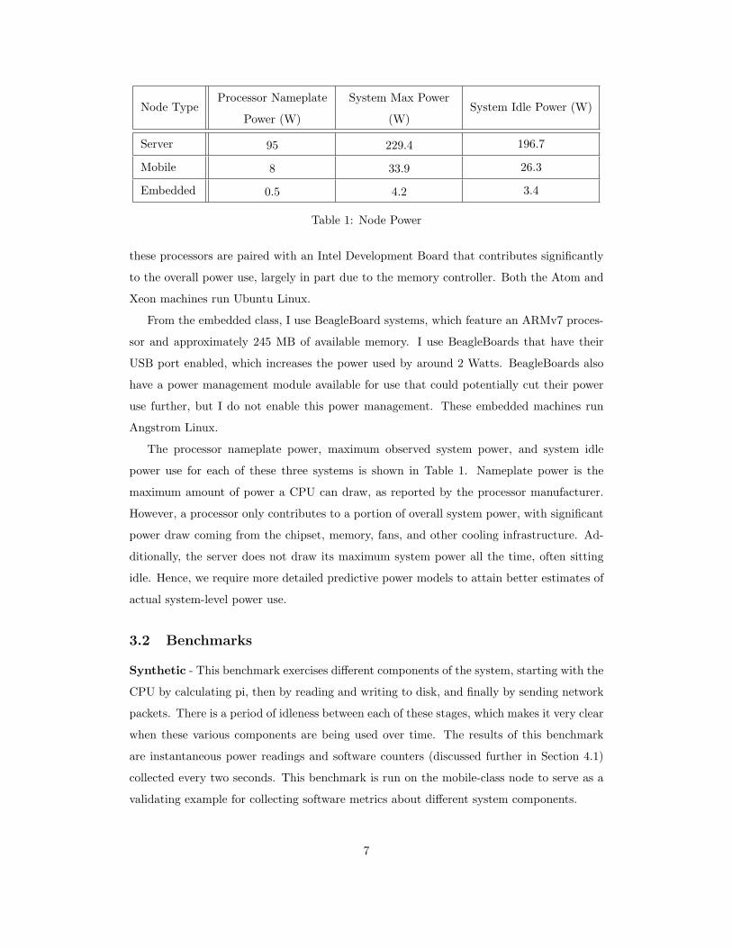
The processor nameplate power, maximum observed system power, and system idle
power use for each of these three systems is shown in Table 1. Nameplate power is the
maximum amount of power a CPU can draw, as reported by the processor manufacturer.
However, a processor only contributes to a portion of overall system power, with significant
power draw coming from the chipset, memory, fans, and other cooling infrastructure. Ad-
ditionally, the server does not draw its maximum system power all the time, often sitting
idle. Hence, we require more detailed predictive power models to attain better estimates of
actual system-level power use.
3.2 Benchmarks
Synthetic - This benchmark exercises different components of the system, starting with the
CPU by calculating pi, then by reading and writing to disk, and finally by sending network
packets. There is a period of idleness between each of these stages, which makes it very clear
when these various components are being used over time. The results of this benchmark
are instantaneous power readings and software counters (discussed further in Section 4.1)
collected every two seconds. This benchmark is run on the mobile-class node to serve as a
validating example for collecting software metrics about different system components.
7
SpecPower - This benchmark exercises the CPU at all different levels of utilization, from
100% down to active idle, and returns power and performance numbers. It is a Java-based
workload with many optimizations available on a per-platform basis, though I use the same
unoptimized program for each platform. This benchmark is run only on the mobile and
server nodes, as there is not currently a good Java installation available for the ARMv7
embedded platform. These results are not considered reportable by the SPEC corporation,
as I do not use SPEC-compliant power and temperature sensors.
Web Server - This benchmark is a real application meant to exercise a web server to its
limits. It uses autobench and httperf to send requests for a 122K web page at increasing
rates to the server under test. The results it gives include average response times, number of
requests received, and number of errors. This test is run across all three hardware platforms,
with the most focus given to the mobile and embedded nodes’ results, the reasons for
which will be discussed further in Section 4.2. Each server-under-test runs lighttpd to serve
its pages, a lighter-weight alternative to Apache. In actual, highly-trafficed web servers,
dynamic requests are generally filled by page caches that return static copies of the most
frequently accessed pages, as is done in this benchmark which makes only static requests.
Batch Sort - This benchmark uses a Hadoop MapReduce distributed sort to represent batch
jobs. The sort occurs over two main stages, a Map and a Reduce phase, with sorted data
sent to other nodes over the network. As such, this benchmark is very network intensive.
The total amount of data sorted depends on the number of nodes involved, with 10 GB of
data allotted per worker or slave node. One node in the cluster must act as the master node
in addition to its role as a worker node, which adds a minimal amount of CPU overhead to
the node with a double-role [3].
3.3 Benchmark Results
The results of the synthetic benchmark show that software counters are indeed good mea-
sures of when a system resource is being utilized. As shown in Figure 1, the CPU test occurs
between seconds 9 and 20 where the CPU line reaches and maintains its peak throughout
the test. The write to disk part of the test occurs at second 26, and the network packets
are sent between seconds 36 and 40. Memory stays constant throughout the whole test, and
network packets are frequently sent and received in small numbers throughout the whole
test as one would expect from a node maintaining its network presence. In addition to the
scripted disk test, there are small numbers of disk writes made frequently throughout the
8
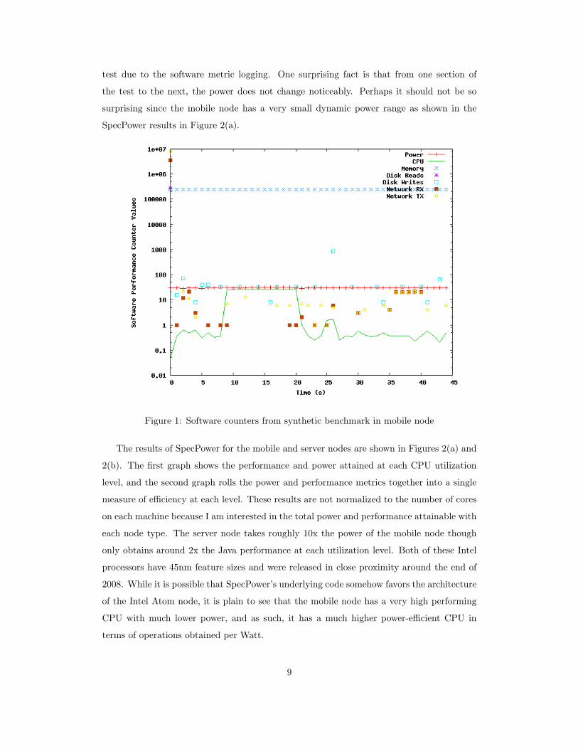
test due to the software metric logging. One surprising fact is that from one section of
the test to the next, the power does not change noticeably. Perhaps it should not be so
surprising since the mobile node has a very small dynamic power range as shown in the
SpecPower results in Figure 2(a).
Figure 1: Software counters from synthetic benchmark in mobile node
The results of SpecPower for the mobile and server nodes are shown in Figures 2(a) and
2(b). The first graph shows the performance and power attained at each CPU utilization
level, and the second graph rolls the power and performance metrics together into a single
measure of efficiency at each level. These results are not normalized to the number of cores
on each machine because I am interested in the total power and performance attainable with
each node type. The server node takes roughly 10x the power of the mobile node though
only obtains around 2x the Java performance at each utilization level. Both of these Intel
processors have 45nm feature sizes and were released in close proximity around the end of
2008. While it is possible that SpecPower’s underlying code somehow favors the architecture
of the Intel Atom node, it is plain to see that the mobile node has a very high performing
CPU with much lower power, and as such, it has a much higher power-efficient CPU in
terms of operations obtained per Watt.
9

Unfortunately, SpecPower results can only be shown for the server and mobile class
devices, as the embedded device is ARMv7-based hardware, which at the time of this writing
does not as yet have a Java implementation. As such, one can only speculate what its CPU
performance and efficiency curves would look like.
Figure 3 shows the response time versus request rate of running the web server application
on each platform. The average response times for each platform are very low until the
platform reaches its respective saturation point or “knee” of operation, in which the server
becomes overloaded, sending response times rocketing. The embedded node can service
up to about 100 requests/second before being overloaded, while the mobile node has its
knee around 500 requests/second, and the Nehalem server responds well until at least 800
requests/second.
4 Power Modeling
The methodology for predictive power modeling is shown in Figure 4. The first step in the
modeling process is a training phase in which a benchmark runs while a collection process
gathers relevant software performance counters and power measurements. These counters
and measurements feed into a statistics program which calculates a linear model that best
fits the input data points. The second testing step is to use these models to predict larger
cluster power usage in an actual web server application. While running the application, I
again collect the software performance counters, but this time, no power meter is needed.
The counters feed into the linear model calculated in the training step and output power
predictions.
4.1 Predicting Mobile Power for Interactive Jobs
While running each of the benchmarks, I periodically collected information from software
counters kept by Linux. Every two seconds I scraped counts for the CPU usage, memory
usage, disk reads and writes (all from /proc/stat), and packets received and transmitted
via the network (netstat) from the time since the last measurement, in addition to the ac-
tual power readings. A significant advantage over using more hardware-based performance
counters is that these software ones are available on every system. While performance coun-
ters really give a better idea of what the underlying hardware is doing (and thus where the
power is actually being consumed), they differ from platform to platform and are notoriously
10
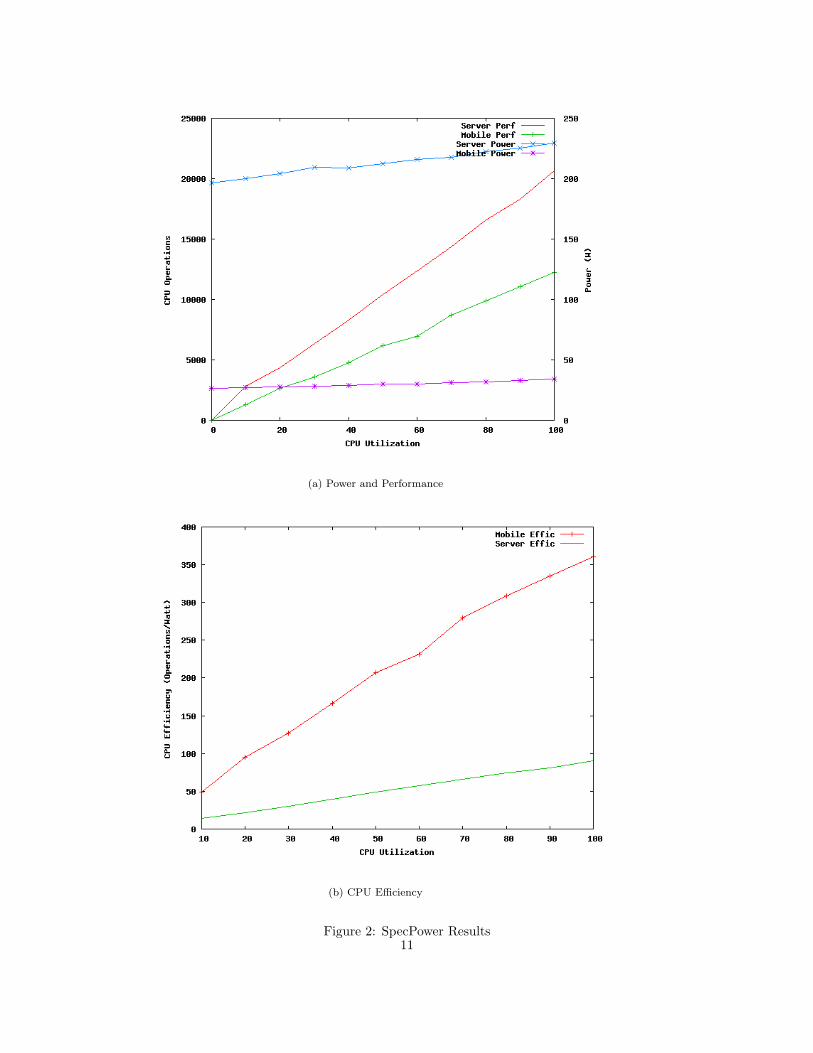
(a) Power and Performance
(b) CPU Efficiency
Figure 2: SpecPower Results11
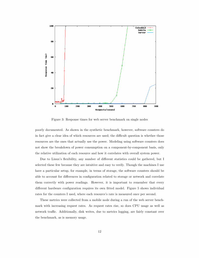
Figure 3: Response times for web server benchmark on single nodes
poorly documented. As shown in the synthetic benchmark, however, software counters do
in fact give a clear idea of which resources are used; the difficult question is whether those
resources are the ones that actually use the power. Modeling using software counters does
not show the breakdown of power consumption on a component-by-component basis, only
the relative utilization of each resource and how it correlates with overall system power.
Due to Linux’s flexibility, any number of different statistics could be gathered, but I
selected these few because they are intuitive and easy to verify. Though the machines I use
have a particular setup, for example, in terms of storage, the software counters should be
able to account for differences in configuration related to storage or network and correlate
them correctly with power readings. However, it is important to remember that every
different hardware configuration requires its own fitted model. Figure 5 shows individual
rates for the counters I used, where each resource’s rate is measured once per second.
These metrics were collected from a mobile node during a run of the web server bench-
mark with increasing request rates. As request rates rise, so does CPU usage as well as
network traffic. Additionally, disk writes, due to metrics logging, are fairly constant over
the benchmark, as is memory usage.
12
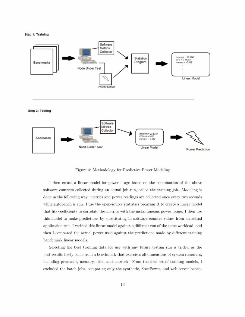
Figure 4: Methodology for Predictive Power Modeling
I then create a linear model for power usage based on the combination of the above
software counters collected during an actual job run, called the training job. Modeling is
done in the following way: metrics and power readings are collected once every two seconds
while autobench is run. I use the open-source statistics program R to create a linear model
that fits coefficients to correlate the metrics with the instantaneous power usage. I then use
this model to make predictions by substituting in software counter values from an actual
application run. I verified this linear model against a different run of the same workload, and
then I compared the actual power used against the predictions made by different training
benchmark linear models.
Selecting the best training data for use with any future testing run is tricky, as the
best results likely come from a benchmark that exercises all dimensions of system resources,
including processor, memory, disk, and network. From the first set of training models, I
excluded the batch jobs, comparing only the synthetic, SpecPower, and web server bench-
13
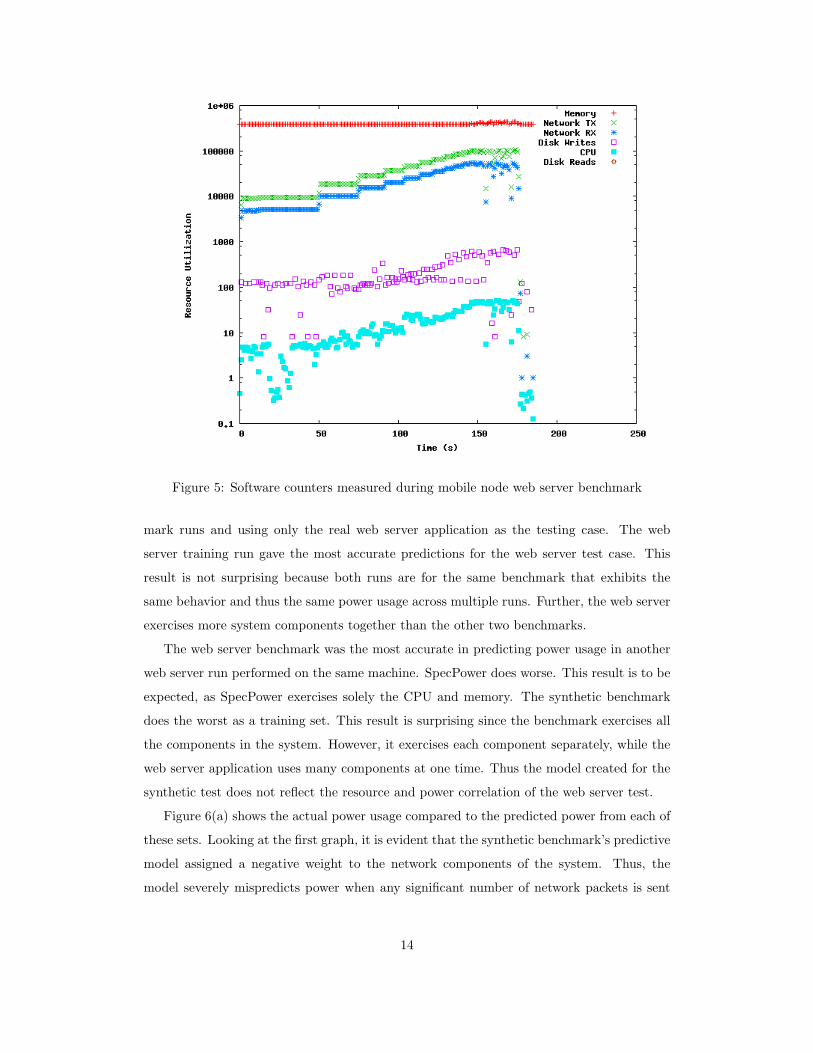
Figure 5: Software counters measured during mobile node web server benchmark
mark runs and using only the real web server application as the testing case. The web
server training run gave the most accurate predictions for the web server test case. This
result is not surprising because both runs are for the same benchmark that exhibits the
same behavior and thus the same power usage across multiple runs. Further, the web server
exercises more system components together than the other two benchmarks.
The web server benchmark was the most accurate in predicting power usage in another
web server run performed on the same machine. SpecPower does worse. This result is to be
expected, as SpecPower exercises solely the CPU and memory. The synthetic benchmark
does the worst as a training set. This result is surprising since the benchmark exercises all
the components in the system. However, it exercises each component separately, while the
web server application uses many components at one time. Thus the model created for the
synthetic test does not reflect the resource and power correlation of the web server test.
Figure 6(a) shows the actual power usage compared to the predicted power from each of
these sets. Looking at the first graph, it is evident that the synthetic benchmark’s predictive
model assigned a negative weight to the network components of the system. Thus, the
model severely mispredicts power when any significant number of network packets is sent
14

or received. Likewise, SpecPower assigned its CPU variable the wrong amount of weight
for a web server test. That is, in a workload that is not strictly-CPU based, its predictions
are inaccurate. The web server prediction is reasonably accurate, falling within 10% of
accuracy of each measured point, which also shows that the web server workload provides
fairly consistent power usage each time it is run.
4.2 Predictions Across Other Architectures
I conducted the same experiments as above on the server and embedded nodes to see if
similar trends arose in the power predictions. The server node shows a large dynamic power
range, stressing the accuracy of the modeling approach. Unfortunately either the underlying
queueing system used by lighttpd or the pen load balancer seems to be a limiting bottleneck
to performance. Thus according to the reported software counters, the server node could
not be pushed beyond more than 10% of its CPU capacity by the web requests to show the
maximum power range.
The different training benchmarks show similar results to those in the mobile node case.
Figure 7(a) shows the results of the different benchmarks’ predictions for the web server
test. SpecPower does the worst in this case. This result is not surprising since the server
node has a much more powerful and power-hungry CPU, meaning that a change in CPU
level can signal a big change in power and should thus be assigned a large coefficient in
the power model. However, a CPU-only benchmark does not work for a network and I/O
utilizing job like the autobench. The synthetic benchmark does not do very well either, again
because it does not utilize individual components at the same time. The web server training
benchmark does remarkably well at predicting the power usage of another web server run.
This result suggests that to get decent power predictions with this software counter setup,
we need to train and test with the same benchmarks.
The embedded board exhibits a dynamic power range of less than one Watt throughout
the entire course of the web server run, as shown in Figure 8. As such, I did not do any
power prediction for the embedded board and instead focus the rest of the power modeling
work on the mobile and server nodes.
15

(a) Actual vs. predicted power
(b) Actual vs. predicted, close-up
Figure 6: Power model comparisons for mobile node web server benchmark16
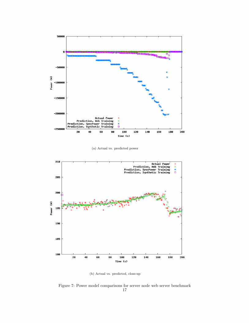
(a) Actual vs. predicted power
(b) Actual vs. predicted, close-up
Figure 7: Power model comparisons for server node web server benchmark17
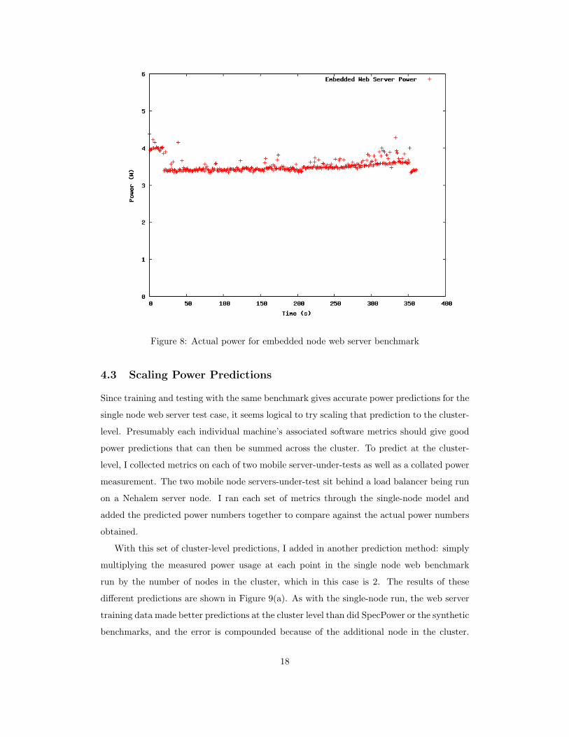
Figure 8: Actual power for embedded node web server benchmark
4.3 Scaling Power Predictions
Since training and testing with the same benchmark gives accurate power predictions for the
single node web server test case, it seems logical to try scaling that prediction to the cluster-
level. Presumably each individual machine’s associated software metrics should give good
power predictions that can then be summed across the cluster. To predict at the cluster-
level, I collected metrics on each of two mobile server-under-tests as well as a collated power
measurement. The two mobile node servers-under-test sit behind a load balancer being run
on a Nehalem server node. I ran each set of metrics through the single-node model and
added the predicted power numbers together to compare against the actual power numbers
obtained.
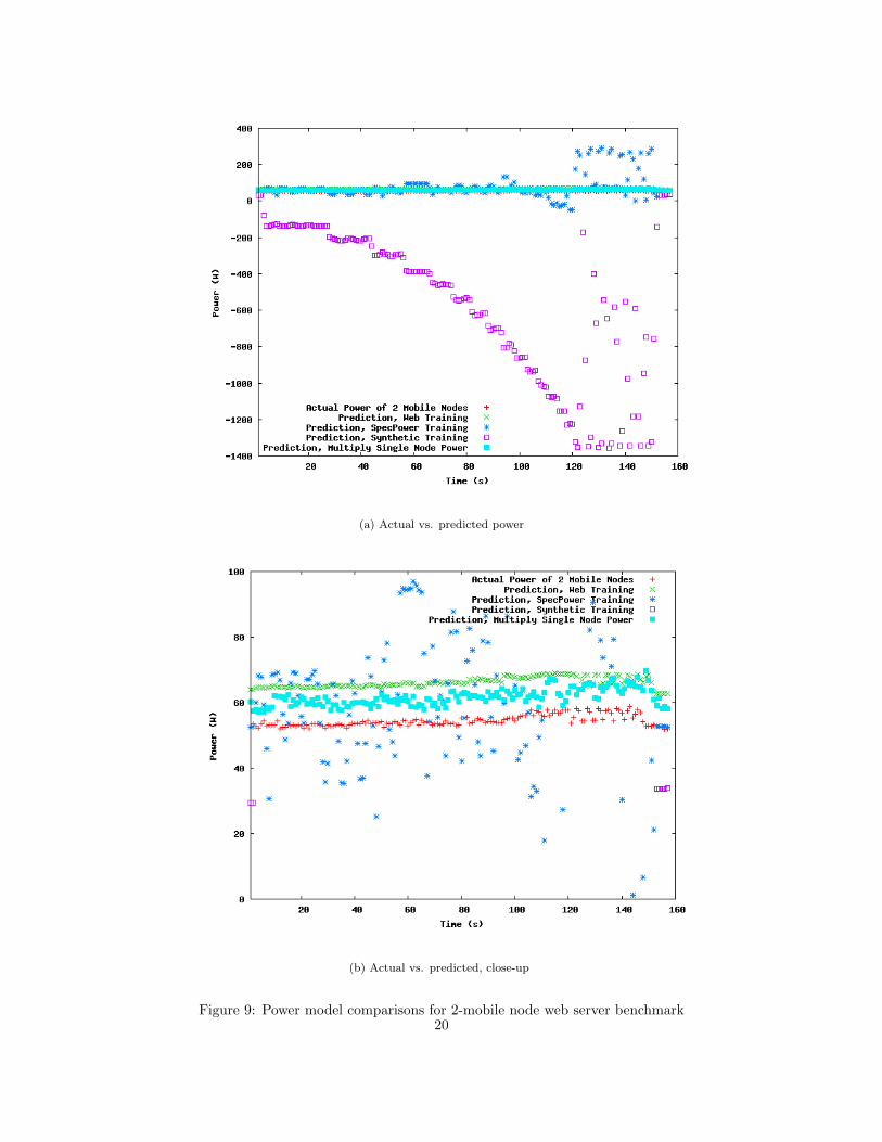
With this set of cluster-level predictions, I added in another prediction method: simply
multiplying the measured power usage at each point in the single node web benchmark
run by the number of nodes in the cluster, which in this case is 2. The results of these
different predictions are shown in Figure 9(a). As with the single-node run, the web server
training data made better predictions at the cluster level than did SpecPower or the synthetic
benchmarks, and the error is compounded because of the additional node in the cluster.
18

However, the simple method of multiplying single node power by 2 performed even better
than the web server prediction did. While the web server prediction falls within 15 to 20%
of the actual power use, the multiply method reaches within 6 to 10% of accuracy at each
point.
In this particular use case, requests are being distributed round-robin, thus causing ho-
mogeneous cluster nodes to have equal resource usage at all times. Workload runs with
homogeneous resource usage across machines, and no modeling is necessary; total cluster
usage can be simply extracted by multiplying out a single node’s power usage. However,
applications with unequal distribution or servers dedicated to running different applications
would need individual power measurements. Batch jobs often distribute tasks across hetero-
geneous machines or with heterogeneous work allocations to each machine and thus provide
a good test case for predicting power based on individual machine’s software counters.
19
(a) Actual vs. predicted power
(b) Actual vs. predicted, close-up
Figure 9: Power model comparisons for 2-mobile node web server benchmark20

4.4 Power Prediction for Batch Jobs
To see how power modeling fares with batch jobs, I run a 10 GB sort across a single
Hadoop node and then scale it up with a sort across two Hadoop slaves nodes with one
slave doubling as a master, collecting software metrics on each machine along with a collated
power measurement.
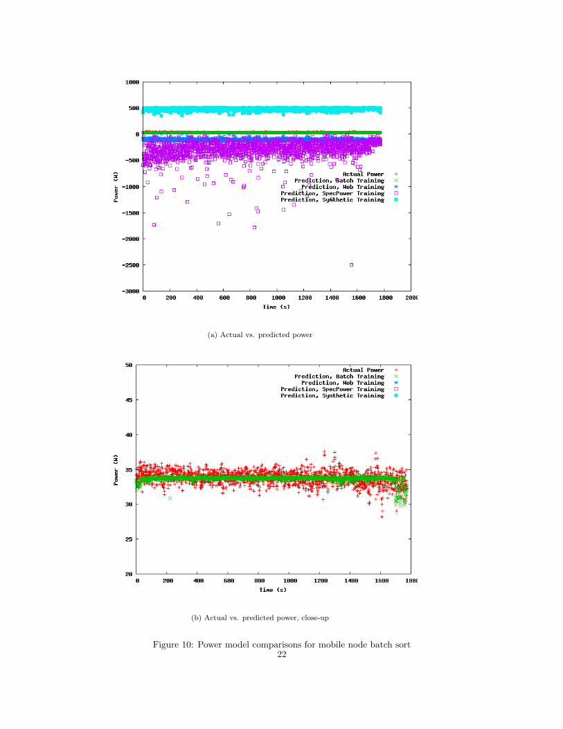
The first batch run was done on a single mobile node. Figure 10(a) shows the actual
and predicted power values from different training benchmarks against a batch run as the
testing benchmark. As with the interactive jobs, SpecPower and the synthetic benchmark
provide poor predictions for the sort job, though the web server application also joins the
ranks in predicting poorly for this job. Figure 10(b) shows that only the batch job does the
trick of predicting power accurately, hitting the average power usage throughout the whole
test and falling within a few Watts of accuracy at every point. However, since the mobile
node only has a small dynamic power range, it is prudent to consider the server node with
a wider power range as well.
The server node exhibits the same behavior, however, with Figure 11(b) showing how
closely the batch training job predicts a different batch testing run with none of the other
three benchmarks even coming close. Additionally, this figure clearly shows the different
power usage for the Map and Reduce phases of the job, with the Map stage completing
around 400 seconds into the run.
To test power prediction at the cluster level for batch jobs, I ran a sort across one server
node and one mobile node together, with the server node acting as the combined master
and slave node. While two servers would have had a greater power range, the shared fan
infrastructure of the servers described earlier would not have allowed for clean predictions,
so I used two completely separate nodes that also happen to be heterogeneous.
The results in Figure 12(a) show a slightly different profile than any previous ones. While
the batch training job from individual nodes comes closest in accuracy for its cluster-level
predictions, the results are not nearly as close as in scaling up the interactive job. So what
changed? In this case, the answer is network traffic.
21
(a) Actual vs. predicted power
(b) Actual vs. predicted power, close-up
Figure 10: Power model comparisons for mobile node batch sort22
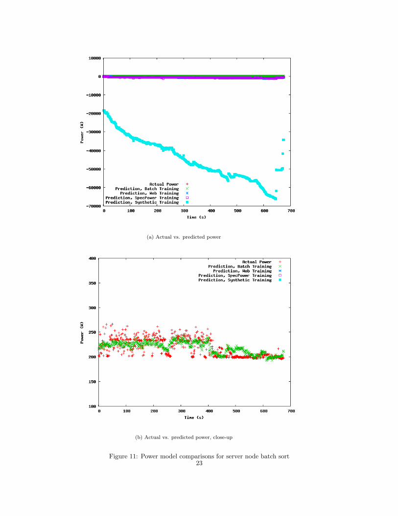
(a) Actual vs. predicted power
(b) Actual vs. predicted power, close-up
Figure 11: Power model comparisons for server node batch sort23
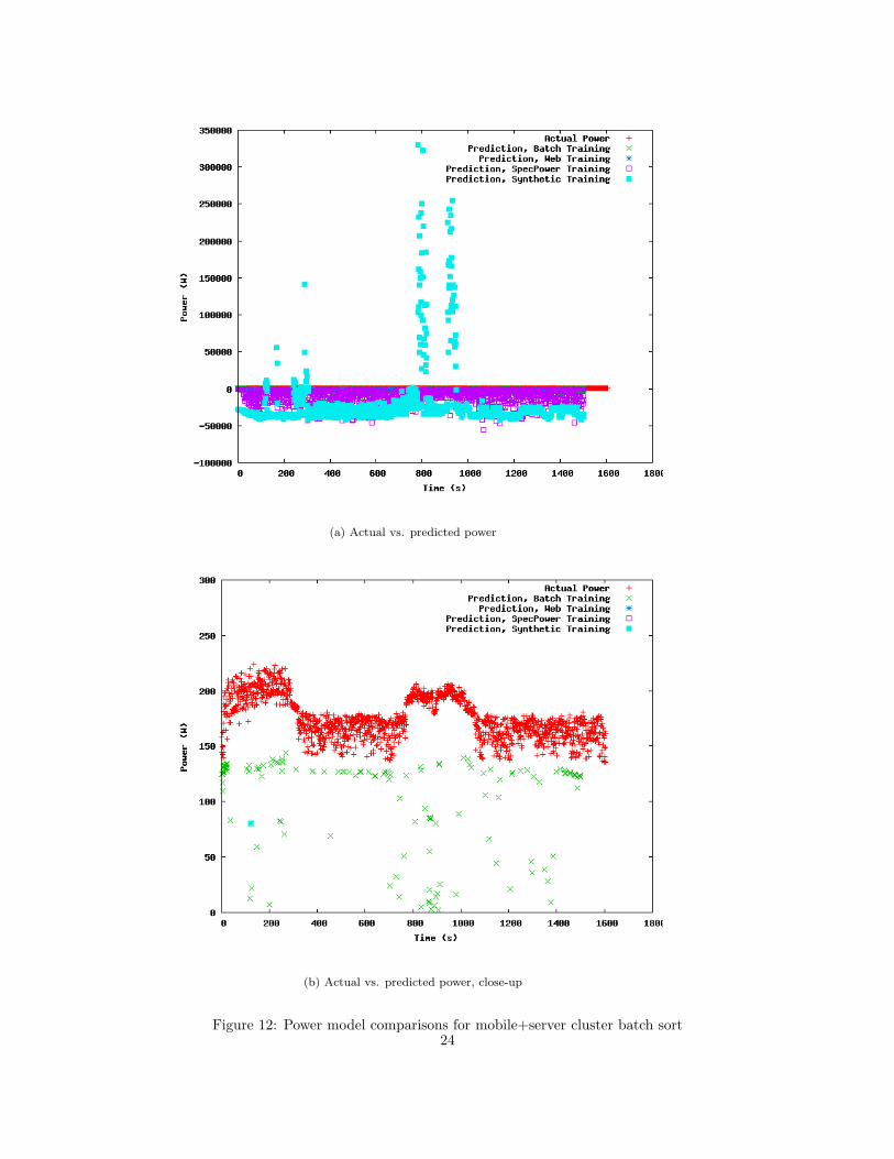
(a) Actual vs. predicted power
(b) Actual vs. predicted power, close-up
Figure 12: Power model comparisons for mobile+server cluster batch sort24
The single node sort jobs created power models without doing any of the requisite net-
work sending and shuffling associated with a multi-node cluster sort. As such, even though
each node was doing exactly the same work with an added sending step, the power pre-
dictions are different. In essence, scaling up a batch sort from a single node to multiple
nodes is almost like running two different programs, at least from the perspective of utilized
resources. When interactive web server tasks are load balanced across multiple machines,
each machine does the same thing it did as a single node without additional steps.
Based on scaling up both interactive and batch job power predictions, there is a big
conclusion we can draw about power modeling using Linux software counters: to get accurate
power predictions, it is important that the training program be very similar to the testing
program. If the profile of resource utilization of any parameter in the linear model changes
significantly from training to testing, the results will be very skewed. In the case of the
batch job, since the server node was responsible for dealing with the network shuffling part
of the sort, its network packets soared, while its overall power didn’t change that much from
its original power use. However, the linear model for the single-node Hadoop server scenario
assigned a coefficient value to the network activity that assumed a low level of network
traffic, so the prediction is totally off in a true multi-node system.
5 Modeling Web Server Performance
In scaling up a cluster, we must consider both how power scales and also how performance is
affected by the addition of nodes. In the case of the real web server application, performance
is measured by average response time, which could be particularly affected by the addition
of heterogeneous nodes.
I used the afore-described web server setup with autobench and lighttpd to fetch a given
file at increasing rates to find the “knee” of a cluster, or the rate at which the response time
increases exponentially, in addition to the average response times. The architecture for the
load balanced web server is shown in Figure 13. Each machine under test sits behind the
open-source load balancer pen on a Nehalem server, and the web workload is generated on an
additional machine. Pen adds minimal overhead at the request rates sent to the individual
machines.
25
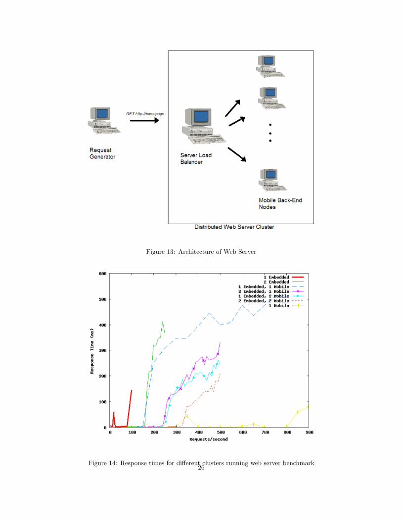
Figure 13: Architecture of Web Server
Figure 14: Response times for different clusters running web server benchmark26

As shown in Figure 14, response time is largely determined by the “weakest,” lowest-
performing member of the cluster. Cluster setups with embedded nodes have their knees at
much lower rates than those without embedded nodes. Additionally, clusters with embedded
nodes have higher knees as their overall cluster size increases. The new cluster knee will
occur at n * {the knee rate of the weakest node}, with the knee’s slope increasing more
gradually the more nodes n there are in the cluster. This knee makes sense because in a
round robin style cluster, one out of every n requests are being sent to each node, meaning the
earliest individual node to reach its knee rate k will occur at the overall cluster request rate
of n * k. Even though the weakest machine’s response time will be increasing exponentially,
the remaining n-1 nodes help to reduce the average response times slightly, meaning that
sufficiently large numbers of machines can help hide the latency imposed by a low-performing
machine.
For higher numbers of n, the slope of the knee will increasingly lessen as the weakest
machine gets requests less often in round-robin mode, though this cannot be shown for
sufficiently high number of requests due to limitations of the load balancer, as discussed in
Section 6.
The average response time reported by httperf can be approximated as follows: the
average response time at a given rate is the average of the response times across all the
machines in the cluster for the rate at 1/nth the total cluster workload rate, that is, at the
incoming rate each individual machine sees.
For a given rate r and n total machines,
avgR(r) =∑n
i Ri( rn )
n(1)
Figure 15 shows the average response time prediction using Equation 1 versus the actual
average response times for two different cluster setups. The first cluster setup is composed
of two embedded nodes, and the second is one embedded node and two mobile nodes. The
predicted response times very closely approximate the actual response times, though the
slope of the actual response times seems a bit smoother than the slopes of the predicted
times. This discrepancy requires further study though is likely due to the presence of a
load balancer, with overloaded nodes able to empty their queues slightly during micro- or
millisecond delays introduced by the load balancer, thus reducing the average response time
by a few milliseconds.
27
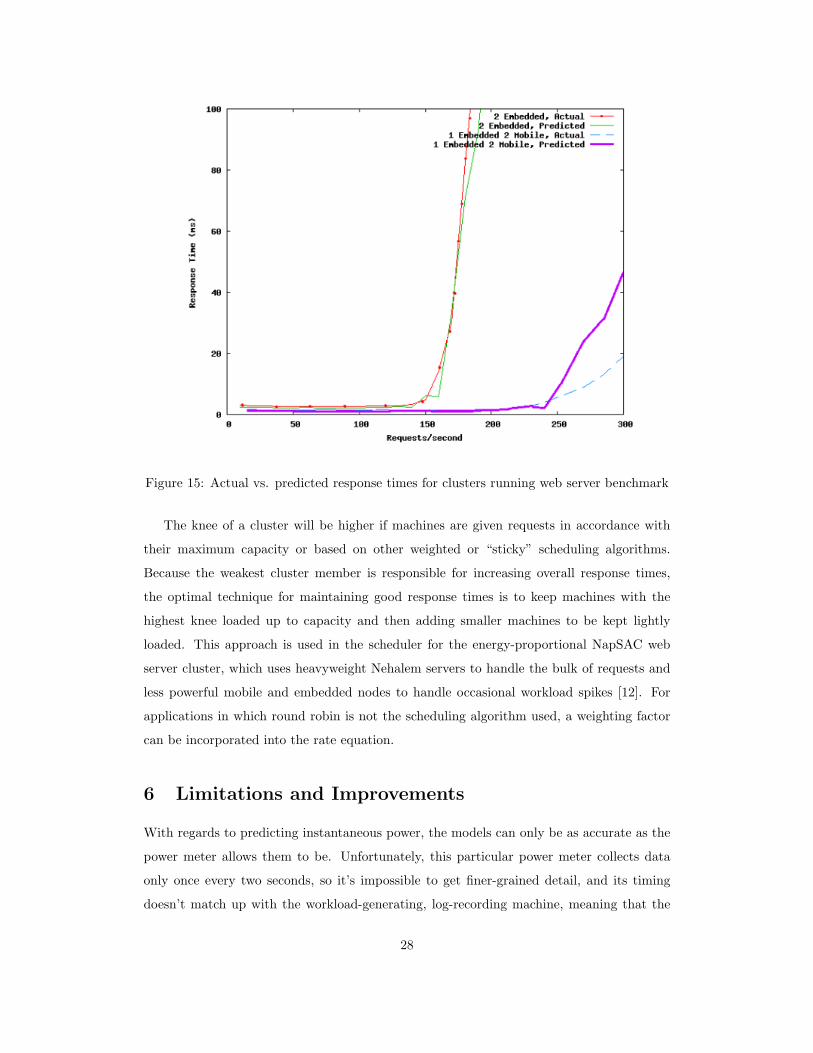
Figure 15: Actual vs. predicted response times for clusters running web server benchmark
The knee of a cluster will be higher if machines are given requests in accordance with
their maximum capacity or based on other weighted or “sticky” scheduling algorithms.
Because the weakest cluster member is responsible for increasing overall response times,
the optimal technique for maintaining good response times is to keep machines with the
highest knee loaded up to capacity and then adding smaller machines to be kept lightly
loaded. This approach is used in the scheduler for the energy-proportional NapSAC web
server cluster, which uses heavyweight Nehalem servers to handle the bulk of requests and
less powerful mobile and embedded nodes to handle occasional workload spikes [12]. For
applications in which round robin is not the scheduling algorithm used, a weighting factor
can be incorporated into the rate equation.
6 Limitations and Improvements
With regards to predicting instantaneous power, the models can only be as accurate as the
power meter allows them to be. Unfortunately, this particular power meter collects data
only once every two seconds, so it’s impossible to get finer-grained detail, and its timing
doesn’t match up with the workload-generating, log-recording machine, meaning that the
28

number of metrics and power readings do not match up exactly, which makes it difficult to
create an accurate model as some readings must be thrown out. Synching up the CPU and
power meter is sadly out of my hands, as I do not know of any way to calibrate the timing
on this power meter. The description of the power meter as taking readings “every two
seconds” is fairly generous, as it does not seem to maintain a reliable two second interval,
with variations of milliseconds building up with each measurement. I can only assume that
the actual Watt measurements it provides are accurate at all levels, as I have not physically
calibrated it myself.
Improving the actual power model for predictions where nodes are not equally utilized
could entail splitting up the model into two parts, one to handle the high end of the CPU
spectrum and the other to handle the lower half, based on some empirically discovered
inflection point. Additionally, different methods of measuring the CPU utilization or mea-
suring at longer intervals is also possible, though the latter option doesn’t seem to help
much due to the afore-mentioned power meter limitations. Realistically, improvements to
power modeling simply cannot happen without first finding a top-notch power meter.
Non-linear models, particularly within certain components like the CPU, seem to be
pointed at by work by Rivoire et al. Also, CPU utiilization on multicore machines is
measured based on average combined utilization across all cores, so different cores are at
different utilization levels. It would be possible to add additional counters for each core, but
the models using similar training and testing workloads are accurate enough without these
individual counters.
Turning to performance modeling, the load balancer is itself a limitation. It has an
inherent limit to how many requests it can handle, based on operating system settings,
link capacity, and CPU capabilities of the hosting machine. Ideal load balancing allows
us to find the knee of cluster operations, but available load balancers often fall short of
this expectation without significant tinkering and recompiling of the OS. We are ultimately
limited by the underlying machine running the load balancer, so the solution to this problem
is to use a high-performing machine to load balance, or better yet, to use many machines
together as a load balancer. Finding the actual cluster knee would require a much higher
performing node, so I conducted my load balancing experiments with the smaller capacity
embedded and mobile nodes and hope that their behavior generalizes to the server class.
It is impossible to do any experiments over 850 requests/second, though it is hard to say
whether this limit is due more to the load balancer’s lack of robustness or the actual server
node itself (though the overhead associated with using the load balancer appears to be fairly
29
minimal at low request rates).
7 Visualizer
7.1 A Tool for Visualizing Energy-Aware Configurations
The above benchmarks and tests show that cluster energy usage varies drastically depending
on the individual components it is composed of due to different power and performance
capabilities of the individual cluster building blocks. To make it easier to see these differences
before actually having to physically build and test a cluster, I present a Cluster Visualizer
GUI.
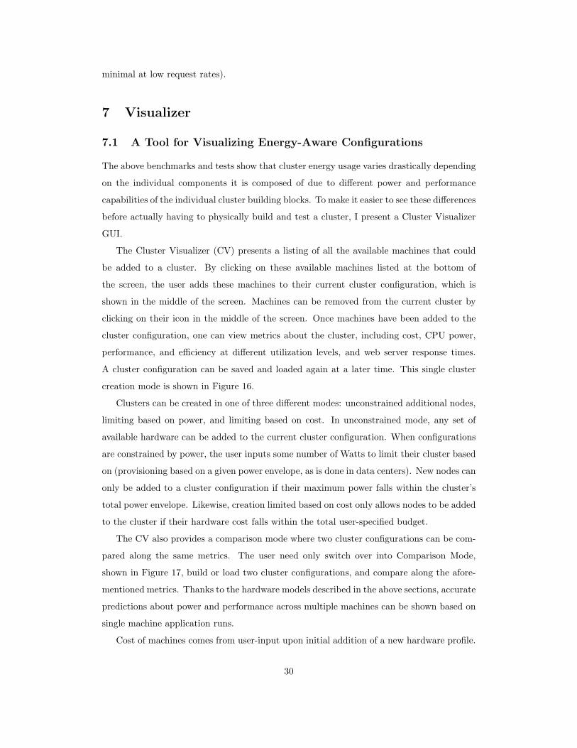
The Cluster Visualizer (CV) presents a listing of all the available machines that could
be added to a cluster. By clicking on these available machines listed at the bottom of
the screen, the user adds these machines to their current cluster configuration, which is
shown in the middle of the screen. Machines can be removed from the current cluster by
clicking on their icon in the middle of the screen. Once machines have been added to the
cluster configuration, one can view metrics about the cluster, including cost, CPU power,
performance, and efficiency at different utilization levels, and web server response times.
A cluster configuration can be saved and loaded again at a later time. This single cluster
creation mode is shown in Figure 16.
Clusters can be created in one of three different modes: unconstrained additional nodes,
limiting based on power, and limiting based on cost. In unconstrained mode, any set of
available hardware can be added to the current cluster configuration. When configurations
are constrained by power, the user inputs some number of Watts to limit their cluster based
on (provisioning based on a given power envelope, as is done in data centers). New nodes can
only be added to a cluster configuration if their maximum power falls within the cluster’s
total power envelope. Likewise, creation limited based on cost only allows nodes to be added
to the cluster if their hardware cost falls within the total user-specified budget.
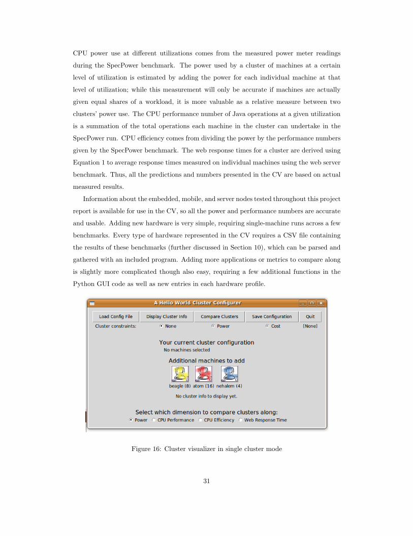
The CV also provides a comparison mode where two cluster configurations can be com-
pared along the same metrics. The user need only switch over into Comparison Mode,
shown in Figure 17, build or load two cluster configurations, and compare along the afore-
mentioned metrics. Thanks to the hardware models described in the above sections, accurate
predictions about power and performance across multiple machines can be shown based on
single machine application runs.
Cost of machines comes from user-input upon initial addition of a new hardware profile.
30
CPU power use at different utilizations comes from the measured power meter readings
during the SpecPower benchmark. The power used by a cluster of machines at a certain
level of utilization is estimated by adding the power for each individual machine at that
level of utilization; while this measurement will only be accurate if machines are actually
given equal shares of a workload, it is more valuable as a relative measure between two
clusters’ power use. The CPU performance number of Java operations at a given utilization
is a summation of the total operations each machine in the cluster can undertake in the
SpecPower run. CPU efficiency comes from dividing the power by the performance numbers
given by the SpecPower benchmark. The web response times for a cluster are derived using
Equation 1 to average response times measured on individual machines using the web server
benchmark. Thus, all the predictions and numbers presented in the CV are based on actual
measured results.
Information about the embedded, mobile, and server nodes tested throughout this project
report is available for use in the CV, so all the power and performance numbers are accurate
and usable. Adding new hardware is very simple, requiring single-machine runs across a few
benchmarks. Every type of hardware represented in the CV requires a CSV file containing
the results of these benchmarks (further discussed in Section 10), which can be parsed and
gathered with an included program. Adding more applications or metrics to compare along
is slightly more complicated though also easy, requiring a few additional functions in the
Python GUI code as well as new entries in each hardware profile.
Figure 16: Cluster visualizer in single cluster mode
31
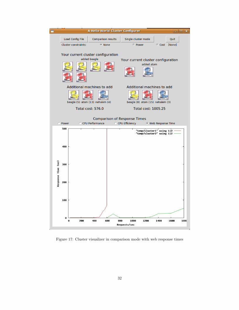
Figure 17: Cluster visualizer in comparison mode with web response times
32
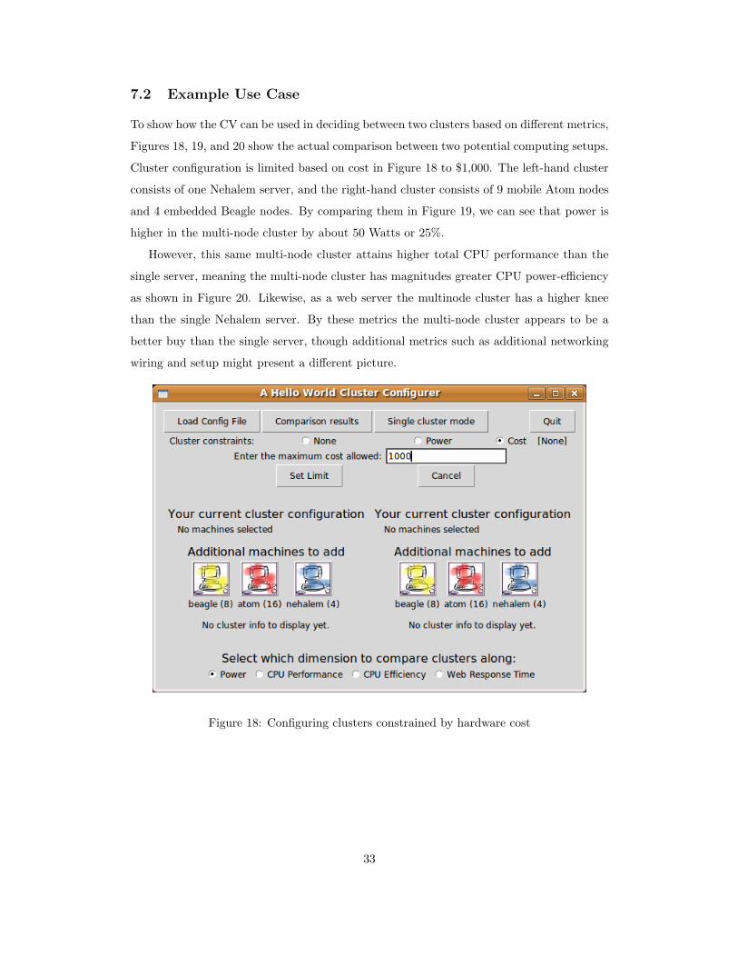
7.2 Example Use Case
To show how the CV can be used in deciding between two clusters based on different metrics,
Figures 18, 19, and 20 show the actual comparison between two potential computing setups.
Cluster configuration is limited based on cost in Figure 18 to $1,000. The left-hand cluster
consists of one Nehalem server, and the right-hand cluster consists of 9 mobile Atom nodes
and 4 embedded Beagle nodes. By comparing them in Figure 19, we can see that power is
higher in the multi-node cluster by about 50 Watts or 25%.
However, this same multi-node cluster attains higher total CPU performance than the
single server, meaning the multi-node cluster has magnitudes greater CPU power-efficiency
as shown in Figure 20. Likewise, as a web server the multinode cluster has a higher knee
than the single Nehalem server. By these metrics the multi-node cluster appears to be a
better buy than the single server, though additional metrics such as additional networking
wiring and setup might present a different picture.
Figure 18: Configuring clusters constrained by hardware cost
33
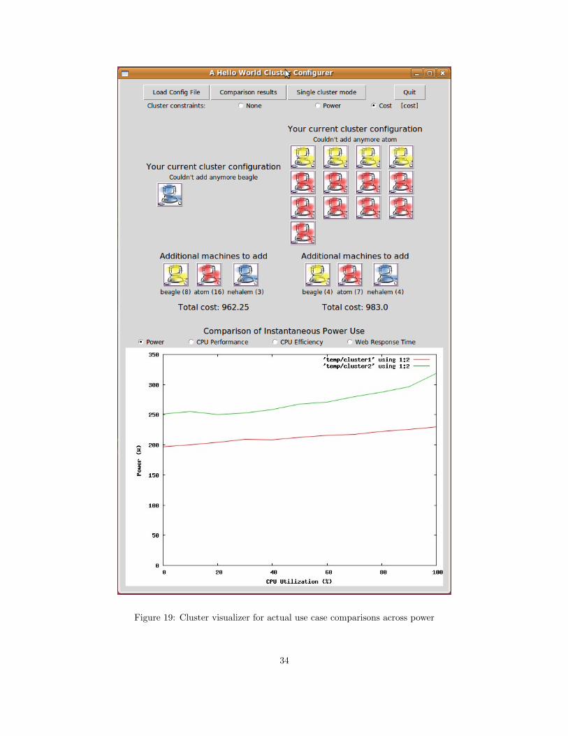
Figure 19: Cluster visualizer for actual use case comparisons across power
34
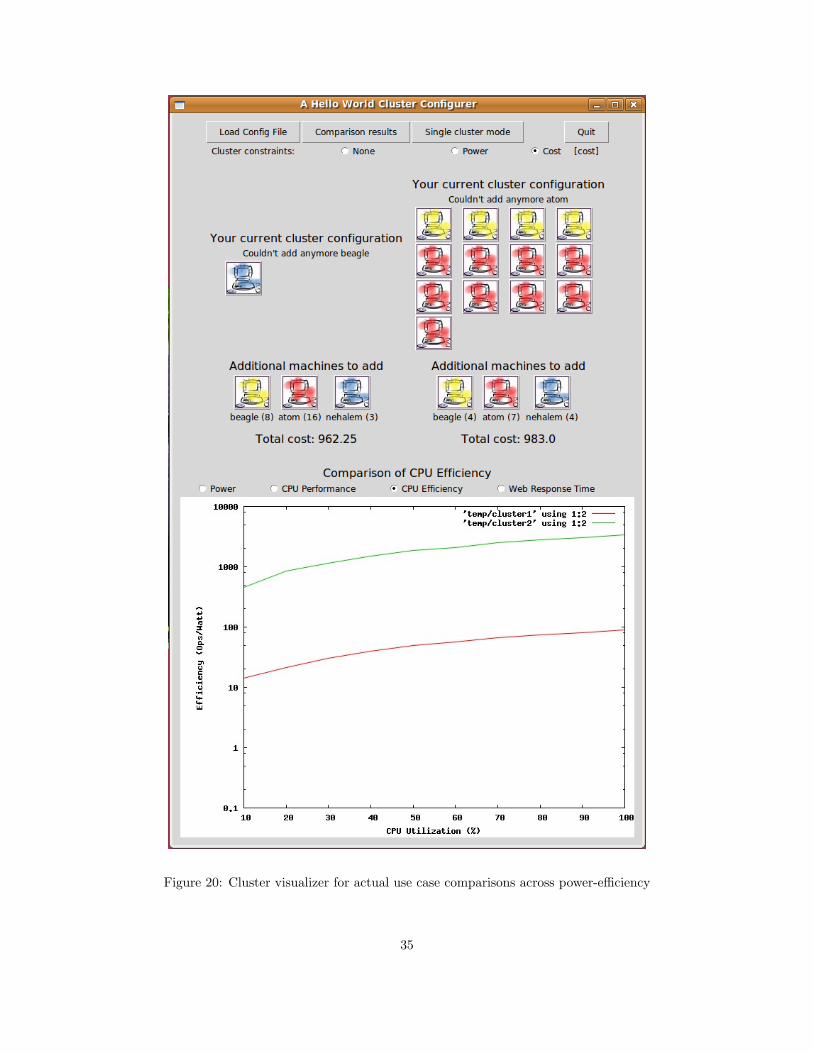
Figure 20: Cluster visualizer for actual use case comparisons across power-efficiency
35

8 Conclusion
Servers in distributed computing environments spend around half their time being lightly
utilized or idle, but they consume more than half of their maximum power in these periods
of low utilization. Thus, power savings in a data center can be achieved without turning ma-
chines off simply by replacing these traditional servers with lower power hardware that will
waste less power when idling. However, deciding which hardware to use in place of servers
is a difficult decision partly because lower power typically equates to lower performance and
also because different cluster owners use different metrics of success in quantifying cluster
performance.
I compared three very different types of hardware across a few benchmarks: an ARM-
based embedded board, an Intel Atom mobile node, and a Xeon server. A selection of
single-machine benchmarks helped build up a profile of each type of hardware, including
the CPU-intensive SpecPower, a full-system synthetic benchmark, the web server autobench,
and a MapReduce batch sort. Comparing the three systems across power use, traditional
performance, efficiency, and response times, the mobile node exhibited the highest efficiency
by using considerably lower power than the traditional server while still being able to main-
tain reasonable performance.
From these single-machine benchmark runs, I created a linear hardware model that in-
corporates OS-reported metrics about CPU, memory, disk, and network utilization for each
machine type and compared the power predictions from these models against homogeneous
clusters of each machine type. Ultimately, this software-based modeling method seems to
give accurate results only when the type of workload being predicted very closely matches
the training workload on which the model was based. Additionally, I modeled the per-
formance of heterogeneous clusters acting as a load-balanced web server and found that
average response time is easily and accurately modeled based on single-machine runs for
each hardware type in the cluster.
I also presented a Cluster Visualizer GUI for comparing potential clusters consisting of
different types of machines. These imaginary clusters can be created without any restrictions
or can be constrained based on a power envelope or on a limit of the monetary cost of the
hardware. Two clusters can be compared side-by-side based on power use at different
levels of resource utilization, traditional performance numbers, power efficiency based on
operations per Watt, or average response times when acting as a web server. All numbers
in the visualizer come from the benchmarks I ran and were verified against scaled-up cluster
runs of the same benchmarks and thus are representative of real performance and power
36
achievable within a homogeneous cluster. This visualizer makes it easier to compare new
sets of hardware to traditional servers along different axes to see if the alternative hardware
can obtain the same level of service previously offered by the servers.
9 Acknowledgements
This project could not have been seen to completion without the assistance and support of
numerous individuals and groups. Thanks to Randy H. Katz for direction and guidance on
this project and to David Culler for his valuable input. Many thanks to the indispensible
Albert Goto and Jon Kuroda for their fast, effective help in getting systems up and keeping
them running. Further thanks go out to Stephen Dawson-Haggerty for his help in dealing
with various power meters, to Yanpei Chen for initially laying the groundwork for investi-
gating power-efficiency in Hadoop, to John Davis and Suzanne Rivoire for their part in the
initial cluster comparison and modeling work, and to Ken Lutz and the SIGCluster group
for their efforts in creating an energy-proportional cluster on which to conduct research.
Final thanks to all the LoCal-ers and others who gave feedback and encouragement along
the way. This work was made possible by a fellowship from NDSEG.
References
[1] D. Andersen, J. Franklin, et al., “FAWN: a fast array of wimpy nodes,” in Proc. of the
22nd ACM Symp. on Operating Systems Principles (SOSP), Big Sky, MT, Oct. 2009.
[2] L.A. Barroso, U. Hoelzle, “The case for energy-proportional computing,” IEEE Com-
puter, vol. 40, no. 12, Dec. 2007, pp. 33-37.
[3] Y. Chen, L. Keys, R. Katz, “Towards Energy Efficient MapReduce,” Technical report,
University of California at Berkeley, August 2009.
[4] D. Economou, S. Rivoire, et al., “Full-system power analysis and modeling for server
environments,” in Proceedings of the Workshop on Modeling, Benchmarking, and Sim-
ulation (MoBS), June 2006.
[5] R. Guerra, J. Leite, G. Fohler, “Attaining Soft Real-Time Constraint and Energy-
Efficiency in Web Servers,” in ACM Symposium on Applied Computing (SAC), 2008.
37

[6] J. Hamilton, “CEMS: low-cost, low-power servers for internet-scale services,” in Proc. of
the 4th Bienneial Conference on Innovative Data Systems Research (CIDR, Asilomar,
CA, Jan. 2009.
[7] T. Heath, B. Diniz, et al, “Energy conservation in heterogeneous server clusters,” in
Proceedings of the Symposium on Principles and Practice of Parallel Programming
(PPoPP), June 2005.
[8] C. Isci and M. Martonosi, “Runtime power monitoring in high-end processors: Method-
ology and empirical data,” in Proc. of the International Symposium on Microarchitec-
ture (MICRO-36), Dec. 2003.
[9] R. Joseph and M. Martonosi, “Run-time power estimation in high performance micro-
processors,” in Proc. of the International Symposium on Low-Power Electronics and
Design (ISLPED), Aug. 2001.
[10] I. Kadayif, T. Chinoda, et al., “vEC: Virtual energy counters,” in Proc. of the ACM
SIGPLAN/SIGSOFT Workshop on Program Analysis for Software Tools and Engineer-
ing (PASTE), June 2001.
[11] L. Keys, S. Rivoire, J. Davis, “The Search for Energy Efficient Cluster Building Blocks”,
in Workshop on Energy Efficient Design (WEED), Saint-Malo, France, June 2010.
[12] A. Krioukov, P. Mohan, S. Alspaugh, L. Keys, D. Culler, R. Katz, “NapSAC: De-
sign and Implementation of a Power Proportional Web Server Cluster,” in First ACM
SIGCOMM Workshop on Green Networking, New Delhi, India, August 2010.
[13] J. Leverich and C. Kozyrakis, “On the energy (in)efficiency of Hadoop clusters,” in
Proc. of the 2nd Workshop on Power-Aware Computing and Systems (HotPower), Big
Sky, MT, Oct. 2009.
[14] K. Lim, P. Ranganathan, et al., “Understanding and designing new server architectures
for emerging warehouse-computing environments,” in Proc. of the 35th Intl. Symp. on
Computer Architecture (ISCA), Beijing, China, June 2008.
[15] V.J. Reddi, B. Lee, et al., “Web search using small cores: quantifying the price of
efficiency,” Microsoft Research Technical Report MSR-TR-2009-105, Aug. 2009.
[16] S. Rivoire, “A Comparison of High-Level Full-System Power Models,” in Proc. of the
1st Workshop on Power-Aware Computing and Systems (HotPower), 2008.
38

[17] S. Rivoire, M.A. Shah, P. Ranganathan, C. Kozyrakis, “JouleSort: A Balanced Energy-
Efficiency Benchmark,” in ACM SIGMOD, Beijing, China, June 2007.
[18] US Environmental Protection Agency (EPA), ENERGY STAR Program, “Report to
Congress on Server and Data Center Energy Efficiency”, Public Law 109-431, August
2007.
10 Appendix
The hardware presented in the cluster is easily configurable, and new machine types can be
easily added through the included Python script.
The inputs to the CV are a .profile CSV for each type of hardware available. Each line
in the .profile for a piece of hardware is preceded by a tag for its associated benchmark.
The following formats are used for each benchmark or other information:
SpecPower
cpu:<utilization>,<number of operations>,<power>,<operations per Watt>
Web Server
web:<rate>,<resp time>
Number of machines of this hardware type
total machines=<number machines>
Hardware Cost
cost=<amount>
To obtain results for SpecPower entries, you should collect power measurements while
you run the included SpecPower run-all script on a machine of the new hardware type you
would like to add. After the run is complete, you will need to locate the Results folder and
find the ssj-*-.raw file. Save that somewhere handy, along with the file where you collected
all the power measurements.
Web server entries can be obtained by running the included autobench script. In the
autobench script, you should set the command line option “–file=¡filename¿” to a file name
of your choice. Save that file somewhere handy after the run is complete.
After running the SpecPower and autobench tests, you should run the create-profile.py
script and then input the locations of the necessary files when asked for them. The script
39

will parse your files and add them to the new hardware .profile, which will be used the next
time you open the CV GUI.
40