A Model-Based Frequency Constraint for Mining …michael.hahsler.net/research/nbd_dami2005/NBD_print.pdf · Both rely only on the conﬁdence measure deﬁned for association rules

Data Mining and Knowledge Discovery, 13, 137–166, 2006c© 2006 Springer Science + Business Media, LLC. Manufactured in the United States.

DOI: 10.1007/s10618-005-0026-2

A Model-Based Frequency Constraint for MiningAssociations from Transaction DataMICHAEL HAHSLER [email protected] University of Economics and Business Administration,

Received April 19, 2005; Accepted October 20, 2005

Published online: 12 May 2006

Abstract. Mining frequent itemsets is a popular method for finding associated items in databases. For thismethod, support, the co-occurrence frequency of the items which form an association, is used as the primaryindicator of the associations’s significance. A single, user-specified support threshold is used to decided ifassociations should be further investigated. Support has some known problems with rare items, favors shorteritemsets and sometimes produces misleading associations.

In this paper we develop a novel model-based frequency constraint as an alternative to a single, user-specifiedminimum support. The constraint utilizes knowledge of the process generating transaction data by applying asimple stochastic mixture model (the NB model) which allows for transaction data’s typically highly skeweditem frequency distribution. A user-specified precision threshold is used together with the model to find localfrequency thresholds for groups of itemsets. Based on the constraint we develop the notion of NB-frequentitemsets and adapt a mining algorithm to find all NB-frequent itemsets in a database. In experiments withpublicly available transaction databases we show that the new constraint provides improvements over a singleminimum support threshold and that the precision threshold is more robust and easier to set and interpret bythe user.

Keywords: Data mining, associations, interest measures, mixture models, transaction data.

1. Introduction

Mining associations (i.e., set of associated items) in large databases has been underintense research since Agrawal et al. (1993) presented Apriori, the first algorithm usingthe support-confidence framework to mine frequent itemsets and association rules.Theenormous interest in associations between items is due to their direct applicabilityfor many practical purposes. Beginning with discovering regularities in transaction datarecorded by point-of-sale systems to improve sales, associations are also used to analyzeWeb usage patterns (Srivastava et al., 2000), for intrusion detection (Luo and Bridges,2000), for mining genome data (Creighton and Hanash, 2003), and for many otherapplications.

An association is a set of items found in a database which provides useful andactionable insights into the structure of the data. For most current applications sup-port is used to find potentially useful associations. Support is a measure of sig-nificance defined as the relative frequency of an association in the database. Themain advantages of using support are that it is simple to calculate, no assump-tions about the structure of mined data are required, and support possesses the aso-called downward closure property (Agrawal and Srikant, 1994) which makesa more efficient search for all frequent itemsets in a database possible. However,

138 HAHSLER

support has also some important shortcomings. Some examples found in the litera-ture are:

• Silverstein et al. (1998) argue with the help of examples that the definition of associ-ation rules (using support and confidence) can produce misleading associations. Theauthors suggest using statistical tests instead of support to find reliable dependenciesbetween items.

• Support is prone to the rare item problem (Liu et al., 1999) where associationsincluding items with low support are discarded although they might represent valuableinformation.

• Support favors smaller itemsets while longer itemsets could still be interesting, evenif they are less frequent (Seno and Karypis, 2001). In order to find longer itemset, onewould have to lower the support threshold which would lead to an explosion of thenumber of short itemsets found.

Statistics provides a multitude of models which proved to be extremely helpful todescribe data frequently mined for associations (e.g., accident data, market research dataincluding market baskets, data from medical and military applications, and biometricaldata (Johnson et al., 1993)). For transaction data, many models build on mixtures ofcounting processes which are known to result in extremely skewed item frequencydistributions with very few relatively frequent items while most items are infrequent.This is especially problematic since support’s rare item problem affects the majority ofitems in such a database. Although the effects of skewed item frequency distributionsin transaction data are sometimes discussed (e.g. by Liu et al. (1999) or Xiong et al.(2003)), most current approaches neglect knowledge about statistical properties of thegenerating processes which underlie the mined databases.

The contribution of this paper is that we address the shortcomings of a single, user-specified minimum support threshold by departing from finding frequent itemsets. In-stead we propose a model-based frequency constraint to find NB-frequent itemsets. Forthis constraint we utilizes knowledge of the process which underlies transaction data byapplying a simple stochastic baseline model (an extension of the NB model) which isknown for its wide applicability. A user-specified precision threshold is used to identifylocal frequency thresholds for groups of associations based on evaluating observed de-viations from a baseline model. The proposed model-based constraint has the followingproperties:

1. It reduces the problem with rare items since the used stochastic model allows forhighly skewed frequency distributions.

2. It is able to produce longer associations without generating an enormous number ofshorter, spurious associations since the support required by the model is set locallyand decreases with the number of items forming an association.

3. Its precision threshold parameter can be interpreted as a predicted error rate. Thismakes communicating and setting the parameter easier for domain experts. Also, theparameter seems to be less dependent on the structure of the database than support.

The rest of the paper is organized as follows: In the next section we review thebackground of mining associations and some proposed alternative frequency constraints.

A MODEL-BASED FREQUENCY CONSTRAINT 139

In Section 3 we develop the model-based frequency constraint, the concept of NB-frequent itemsets, and show that the chosen model is useful to describe real-wordtransaction data. In Section 4 we present an algorithm to mine all NB-frequent itemsetsin a database. In Section 5 we investigate and discuss the behavior of the model-basedconstraint using several real-world and artificial transaction data sets.

2. Background and related work

The problem of mining associated items (frequent itemsets) from transaction data wasformally introduced by Agrawal et al. (1993) for mining association rules as:Let I ={i1, i2, . . . , in} be a set of n distinct literals called items and D = {t1, t2, . . . , tm} a setof transactions called the database. Each transaction in D contains a subset of the itemsin I. A rule is defined as an implication of the from X −→ Y where X, Y ⊆ I andX ∩ Y = ∅. The sets of items (for short itemsets) X and Y are called antecedent andconsequent of the rule. An itemset which contains k items is said to have length or sizek and is called a k-itemset. An itemset which is produced by adding a single item toanother itemset is called a 1-extension of the latter itemset.

Constraints on various measures of significance and interest can be used to selectinteresting associations and rules. Agrawal et al. (1993) define the measures support andconfidence for association rules.

Definition 1 (Support). Support is defined on itemset Z ⊆ I as the proportion oftransactions in which all items in Z are found together in the database:

supp(Z ) = freq(Z )

|D| ,

where freq(Z ) denotes the frequency of itemset Z (number of transactions in which Zoccurs) in database D, and |D| is the number of transactions in the database.

Confidence is defined for a rule X −→ Y as the ratio supp(X ∪ Y )/supp(X ). Sinceconfidence is not a frequency constraints we will only discuss support in the following.

An itemset Z is only considered significant and interesting in the association ruleframework if the constraint supp(Z ) ≥ σ holds, where σ is a user-specified minimumsupport. Itemsets which satisfy the minimum support constraint are called frequentitemsets since their occurrence frequency surpasses a set frequency threshold, hencethe name frequency constraint. Some authors refer to frequent itemsets also as largeitemsets (Agrawal et al., 1993) or covering sets (Mannila et al., 1994).

The rational for minimum support is that items which appear more often in thedatabase are more important since, e.g. in a sales setting they are responsible for a highersales volume. However, this rational breaks down when some rare but expensive itemscontribute most to the store’s overall earnings. Not finding associations for such itemsis known as support’s rare item problem (Liu et al., 1999). Support also systematicallyfavors smaller itemsets (Seno and Karypis, 2001). By adding items to an itemset theprobability of finding such longer itemsets in the database can only decrease or, in rarecases, stay the same. Consequently, longer itemsets are less likely to meet the minimumsupport. Reducing minimum support to find longer itemsets normally results in an

140 HAHSLER

explosion of the number of small itemsets found, which makes this approach infeasiblefor most applications.

For all but very small or extremely sparse databases, finding all frequent itemsetsis computationally very expensive since the search space for frequent itemsets growsexponentially with the number of items. However, the minimum support constraintpossesses a special property called downward closure (Agrawal and Srikant, 1994) (alsocalled anti-monotonicity (Pei et al., 2001)) which can be used to make more efficientsearch possible. A constraint is downward closed (anti-monotone) if, and only if, foreach itemset which satisfies the constraint all subsets also satisfy the constraint. Thefrequency constraint minimum support is downward closed since if set X is supportedat a threshold σ , also all its subsets Y ⊂ X , which can only have a higher or thesame support as X, must be supported at the same threshold. This property impliesthat (a) an itemset can only satisfy a downward closed constraint if all its subsetssatisfy the constraint and that (b) if an itemset is found to satisfy a downward closedconstraint all its subsets need no inspection since they must also satisfy the constraint.These facts are used by mining algorithms to reduce the search space which is oftenreferred to as pruning or finding a border in the lattice representation of the searchspace.

Driven by support’s problems with rare items and skewed item frequency distributions,some researchers proposed alternatives for mining associations. In the following we willreview some approaches which are related to this work.

Liu et al. (1999) try to alleviate the rare item problem. They suggest mining itemsetswith individual minimum item support thresholds assigned to each item. Liu et al. (1999)showed that after sorting the items according to their minimum item support a sortedclosure property of minimum item support can be used to prune the search space. Aopen research question is how to determine the optimal values for the minimum itemsupports, especially in databases with many items where a manual assignment is notfeasible.

Seno and Karypis (2001) try to reduce support’s tendency to favor smaller itemsetsby proposing a minimum support which decreases as a function of itemset length.Since this invalidates the downward closure of support, the authors develop a propertycalled smallest valid extension, which can be exploited for pruning the search space.As a proof of concept, the authors present results using a linear function for support.However, an open question is how to choose an appropriate support function and itsparameters.

Omiecinski (2003) introduced several alternative interest measures for associationswhich avoid the need for support entirely. Two of the measures are any- and all-confidence. Both rely only on the confidence measure defined for association rules.Any-confidence is defined as the largest confidence of a rule which can be generatedusing all items from an itemset. The author states that although finding all itemsetswith a set any-confidence would enable us to find all rules with a given minimumconfidence, any-confidence cannot be used efficiently as a measure of interestingnesssince minimum confidence is not downward closed. The all-confidence measure isdefined as the smallest confidence of all rules which can be produced from an set ofassociated items. Omiecinski shows that a minimum constraint on all-confidence isdownward closed and, therefore, can be used for efficient mining algorithms withoutsupport.


Another family of approaches is based on using statistical methods to mine associa-tions. The main idea is to identify associations as significant deviations from a baselinegiven by the assumption that items occur statistically independent from each other. Thesimplest measure to quantify this deviation is interest (Brin et al., 1997) which is oftenalso called lift. Interest for a rule X −→ Y is defined as P(X ∪ Y )/(P(X )P(Y )), wherethe denominator is the baseline probability, the expected probability of the itemset underindependence. Interest is usually calculated by the ratio robs/rexp which are the observedand the expected occurrence counts of the itemset. The ratio is close to one if the itemsetsX and Y occur together in the database as expected under the assumption that they are in-dependent. A value greater than one indicates a positive correlation between the itemsetsand values lesser than one indicate a negative correlation. To smooth away noise for lowcounts in the interest ratio, DuMouchel and Pregibon (2001) developed the empiricalBayes Gamma-Poisson shrinker. However, the interest ratio is not a frequency constraintand does not possess the downward closure property needed for efficient mining.

Silverstein et al. (1998) suggested mining dependence rules using the χ2 test forindependence between items on 2 × 2 contingency tables. The authors use the factthat the test statistic can only increase with the number of items to develop miningalgorithms which rely on this upward closure property. DuMouchel and Pregibon (2001)pointed out that more important than the test statistic is the test’s p-value. Due to theincreasing number of degrees of freedom of the χ2 test the p-value can increase ordecrease with itemset size, which invalidates the upward closure property. Furthermore,Silverstein et al. (1998) mention that a significant problem of the approach is the normalapproximation used in the χ2 test. This can skew results unpredictably for contingencytables with cells with low expectation.

First steps towards the approach presented in this paper were made with two projectsconcerned with finding related items for recommendation systems (Geyer-Schulz et al.,2002, 2003). The used algorithms were based on the logarithmic series distribution(LSD) model which is a simplification of the NB model used in this paper. Also thealgorithms were restricted to find only 2-itemsets. However, the projects showed thatthe approach described in this paper produces good results for real-world applications.

3. Developing a model-based frequency constraint

In this section we build on the idea of discovering associated items with the help ofobserved deviations of co-occurrences from a baseline which is based on independencebetween all items. This is similar to how interest (lift) uses the expected probability ofitemsets under independence to identify dependent itemsets. In contrast to lift and othersimilar measure, we will not estimate the degree of deviation at the level of an individualitemset. Rather, we will evaluate the deviation for the set of all possible 1-extensionsof an itemset together to find a local frequency constraint for these extensions. A 1-extension of an k-itemset is an itemset of size k + 1 which is produced by adding anadditional item to the k-itemset.

3.1. A simple stochastic baseline model

A suitable stochastic item occurrence model for the baseline frequencies needs todescribe the occurrence of independent items with different usage frequencies in a robust

142 HAHSLER

items

trans

actio

ns

i1 i2 i3 ... in

t1

t2

t3

t4 .

.. t

m-1

tm

items

tran

sact

ions

i1 i2 i3 ... in

t1

t2

t3 t4 ... tm-1

tm

0 1 0 ... 1 51 0 0 ... 0 20 1 0 ... 0 10 0 0 ... 0 1. . . .. . . .. . . .1 0 0 ... 1 30 0 1 ... 1 2

. . .

freq 99 201 7 ... 411 50614

timesize

(a) (b)

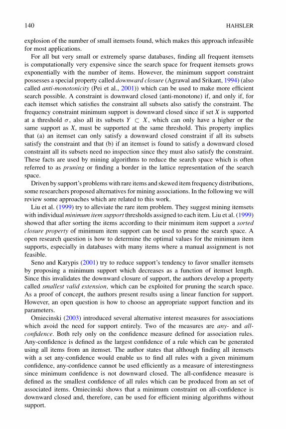
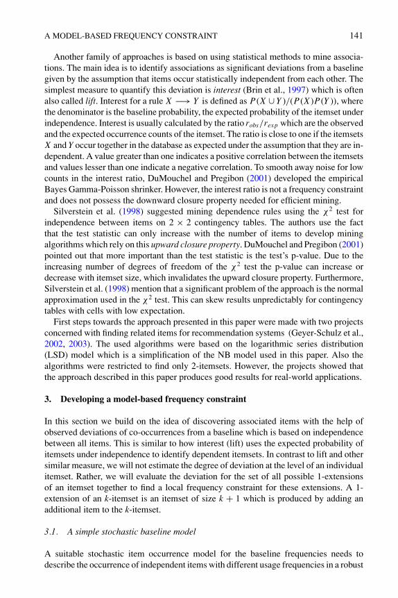
Figure 1. Representation of an example database as (a) sequence of transactions and (b) the incidencematrix.

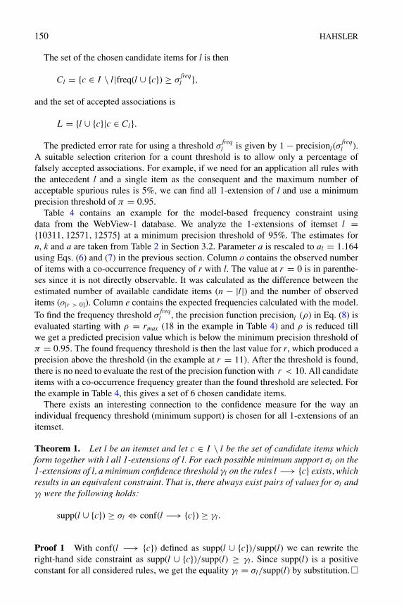
and mathematically tractable way. For the model we consider the occurrence of itemsI = {i1, i2, . . . , in} in a database with a fixed number of m transactions. An exampledatabase is depicted in Figure 1. For the example we use m = 20,000 transactionsand n = 500 items. To the left we see a graphical representation of the database asa sequence of transactions over time. The transactions contain items depicted by thebars at the intersections of transactions and items. The typical representation used fordata mining is the m × n incidence matrix in Figure 1(b). Each row sum representsthe size of a transaction and the column sums are the frequencies of the items in thedatabase. The total sum represents the number of incidences (item occurrences) inthe database. Dividing the number of incidences by the number of transactions givesthe average transaction size (for the example, 50, 614/20,000 = 2.531) and dividingthe number of incidences by the number of items gives the average item frequency(50,614/500 = 101.228).

In the following we will model the baseline for the distribution of the items’ frequencycounts freq in Figure 1(b). For the baseline we suppose that each item in the databasefollows an independent (homogeneous) Poisson process with an individual latent rate λ.Therefore, the frequency for each item in the database is a value drawn from the Poissondistribution with its latent rate. We also assume that the individual rates are randomlydrawn from a suitable distribution defined by the continuous random variable �. Thenthe probability distribution of R, a random variable which gives the number of times anarbitrarily chosen item occurs in the database, is given by

Pr [R = r ] =∫ ∞

0

e−λλr

r !dG�(λ), r = 0, 1, 2, . . . , λ > 0. (1)

This Poisson mixture model results from the continuous mixture of Poisson distribu-tions with rates following the mixing distribution G�.

Heterogeneity in the occurrence frequencies between items is accounted for by theform of the mixing distribution. A commonly used and very flexible mixing distribution


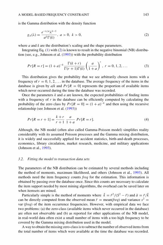
is the Gamma distribution with the density function

g�(λ) = e−λ/aλk−1

ak�(k), a > 0, k > 0, (2)

where a and k are the distribution’s scaling and the shape parameters.Integrating Eq. (1) with (2) is known to result in the negative binomial (NB) distribu-

tion (see, e.g., Johnson et al. (1993)) with the probability distribution

Pr [R = r ] = (1 + a)−k �(k + r )

�(r + 1)�(k)

(a

1 + a

)r

, r = 0, 1, 2, . . . (3)

This distribution gives the probability that we see arbitrarily chosen items with afrequency of r = 0, 1, 2, . . . in the database. The average frequency of the items in thedatabase is given by a/k and Pr [R = 0] represents the proportion of available itemswhich never occurred during the time the database was recorded.

Once the parameters k and a are known, the expected probabilities of finding itemswith a frequency of r in the database can be efficiently computed by calculating theprobability of the zero class by Pr [R = 0] = (1 + a)−k and then using the recursiverelationship (see Johnson et al. (1993))

Pr [R = r + 1] = k + r

r + 1

a

1 + aPr [R = r ]. (4)

Although, the NB model (often also called Gamma-Poisson model) simplifies realityconsiderably with its assumed Poisson processes and the Gamma mixing distribution,it is widely and successfully applied for accident statistics, birth-and-death processes,economics, library circulation, market research, medicine, and military applications(Johnson et al., 1993).

3.2. Fitting the model to transaction data sets

The parameters of the NB distribution can be estimated by several methods includingthe method of moments, maximum likelihood, and others (Johnson et al., 1993). Allmethods need the item frequency counts freq for the estimation. This information isobtained by passing over the database once. Since this counts are necessary to calculatethe item support needed by most mining algorithms, the overhead can be saved later onwhen itemsets are mined.

Particularly simple is the method of moments where k = r2/(S2 − r ) and a = r/kcan be directly computed from the observed mean r = mean(freq) and variance s2 =var (freq) of the item occurrence frequencies. However, with empirical data we facetwo problems: (a) the zero-class (available items which never occurred in the database)are often not observable and (b) as reported for other applications of the NB model,in real-world data often exist a small number of items with a too high frequency to becovered by the Gamma mixing distribution used in the model.

A way to obtain the missing zero-class is to subtract the number of observed items fromthe total number of items which were available at the time the database was recorded.

144 HAHSLER

The number of available items can be obtained from the provider of the database.If the total number of available items is unknown, the size of the zero-class can beestimated together with the parameters of the NB distribution. The standard procedurefor this type of estimation problem is the Expectation Maximization (EM) algorithm(Dempster et al., 1977). This procedure iteratively estimates missing values using theobserved data and the model using intermediate values of the parameters, and then usesthe estimated data and the observed data to update the parameters for the next iteration.The procedure stops when the parameters stabilize. For our estimation problem theprocedure is computationally very inexpensive. Each iteration involves only to calculaten(1+ a)−k to estimate the count for the missing zero-class and then applying the methodof moments (see above) to update the parameter estimates a and k. As we will see inthe examples later in this section, the EM algorithm usually only needs a small numberof iteration to estimate the needed parameters. Therefore, the computational cost ofestimation is insignificant compared to the time needed to count the item frequencies inthe database.

The second estimation problem are outliers with too high frequencies. These outlierswill distort the mean and the variance and thus will lead to a model which grosslyoverestimates the probability of seeing items with high frequencies. For a more robustestimate, we can trim a suitable percentage of the items with the highest frequencies.A suitable percentage can be found by visual comparison of the empirical data and theestimated model or by minimizing the χ2-value of the goodness-of-fit test.

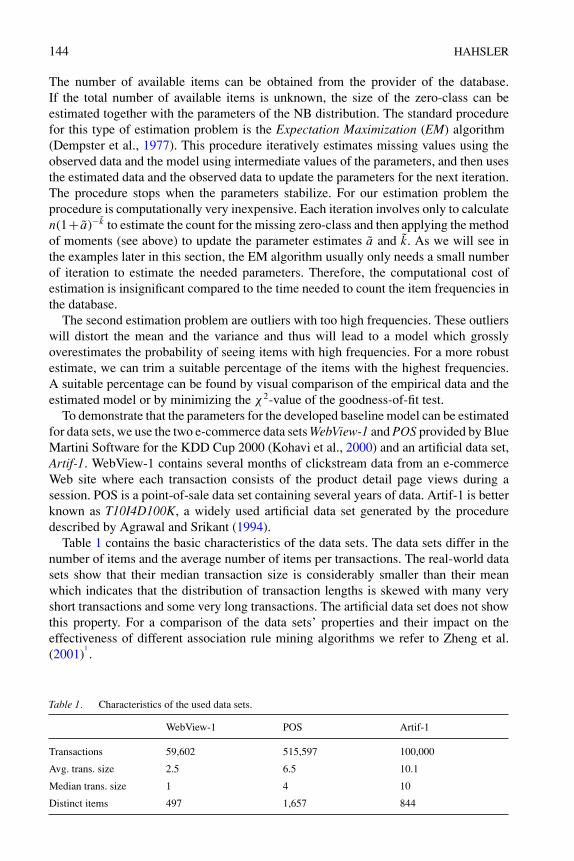
To demonstrate that the parameters for the developed baseline model can be estimatedfor data sets, we use the two e-commerce data sets WebView-1 and POS provided by BlueMartini Software for the KDD Cup 2000 (Kohavi et al., 2000) and an artificial data set,Artif-1. WebView-1 contains several months of clickstream data from an e-commerceWeb site where each transaction consists of the product detail page views during asession. POS is a point-of-sale data set containing several years of data. Artif-1 is betterknown as T10I4D100K, a widely used artificial data set generated by the proceduredescribed by Agrawal and Srikant (1994).

Table 1 contains the basic characteristics of the data sets. The data sets differ in thenumber of items and the average number of items per transactions. The real-world datasets show that their median transaction size is considerably smaller than their meanwhich indicates that the distribution of transaction lengths is skewed with many veryshort transactions and some very long transactions. The artificial data set does not showthis property. For a comparison of the data sets’ properties and their impact on theeffectiveness of different association rule mining algorithms we refer to Zheng et al.(2001)

1.

Table 1. Characteristics of the used data sets.

WebView-1 POS Artif-1

Transactions 59,602 515,597 100,000

Avg. trans. size 2.5 6.5 10.1

Median trans. size 1 4 10

Distinct items 497 1,657 844


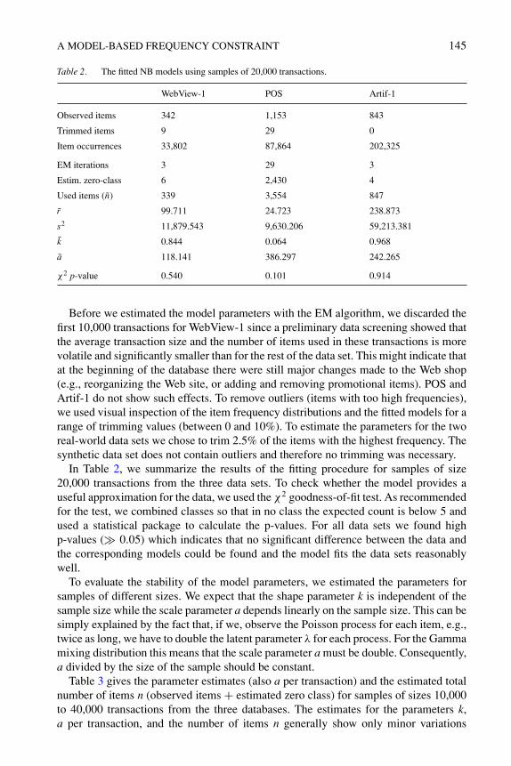
Table 2. The fitted NB models using samples of 20,000 transactions.

WebView-1 POS Artif-1

Observed items 342 1,153 843

Trimmed items 9 29 0

Item occurrences 33,802 87,864 202,325

EM iterations 3 29 3

Estim. zero-class 6 2,430 4

Used items (n) 339 3,554 847

r 99.711 24.723 238.873

s2 11,879.543 9,630.206 59,213.381

k 0.844 0.064 0.968

a 118.141 386.297 242.265

χ2 p-value 0.540 0.101 0.914

Before we estimated the model parameters with the EM algorithm, we discarded thefirst 10,000 transactions for WebView-1 since a preliminary data screening showed thatthe average transaction size and the number of items used in these transactions is morevolatile and significantly smaller than for the rest of the data set. This might indicate thatat the beginning of the database there were still major changes made to the Web shop(e.g., reorganizing the Web site, or adding and removing promotional items). POS andArtif-1 do not show such effects. To remove outliers (items with too high frequencies),we used visual inspection of the item frequency distributions and the fitted models for arange of trimming values (between 0 and 10%). To estimate the parameters for the tworeal-world data sets we chose to trim 2.5% of the items with the highest frequency. Thesynthetic data set does not contain outliers and therefore no trimming was necessary.

In Table 2, we summarize the results of the fitting procedure for samples of size20,000 transactions from the three data sets. To check whether the model provides auseful approximation for the data, we used the χ2 goodness-of-fit test. As recommendedfor the test, we combined classes so that in no class the expected count is below 5 andused a statistical package to calculate the p-values. For all data sets we found highp-values ( 0.05) which indicates that no significant difference between the data andthe corresponding models could be found and the model fits the data sets reasonablywell.

To evaluate the stability of the model parameters, we estimated the parameters forsamples of different sizes. We expect that the shape parameter k is independent of thesample size while the scale parameter a depends linearly on the sample size. This can besimply explained by the fact that, if we, observe the Poisson process for each item, e.g.,twice as long, we have to double the latent parameter λ for each process. For the Gammamixing distribution this means that the scale parameter a must be double. Consequently,a divided by the size of the sample should be constant.

Table 3 gives the parameter estimates (also a per transaction) and the estimated totalnumber of items n (observed items + estimated zero class) for samples of sizes 10,000to 40,000 transactions from the three databases. The estimates for the parameters k,a per transaction, and the number of items n generally show only minor variations

146 HAHSLER

Table 3. Estimates for the NB-model using samples of different sizes.

Name Sample size k aa pertransaction n

WebView-1 10,000 0.933 58.274 0.0058 325

WebView-1 20,000 0.844 118.140 0.0059 339

WebView-1 40,000 0.868 218.635 0.0055 395

POS 10,000 0.060 178.200 0.0178 3,666

POS 20,000 0.064 386.300 0.0193 3,554

POS 40,000 0.064 651.406 0.0163 3,552

Artif-1 10,000 0.975 123.313 0.0123 845

Artif-1 20,000 0.968 242.265 0.0121 847

Artif-1 40,000 0.967 493.692 0.0123 846

over different sample sizes of the same data set. We analyzed the reason for the highjump of the estimated number of items from 339 for 20,000 transactions to 395 for40,000 transactions in WebView-1. We found evidence in the database that after thefirst 20,000 transactions the number of different items in the database starts to grow byabout 10 items every 5,000 transactions. However, this fact does not seem to influencethe stability of the estimates of the parameters k and a. The stability enables us to usemodel parameters estimated for one sample size for samples of different sizes.

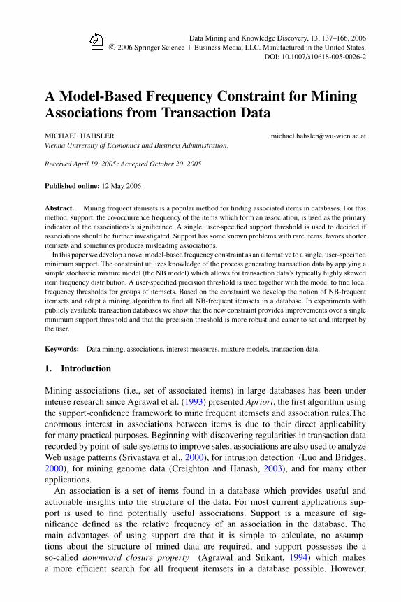
Applied to associations, Eq. (3) in the section above gives the probability distributionof observing single items (1-itemsets) with a frequency of r. Let σ freq = σm, wherem is the number of transactions in the database, be the frequency threshold equivalentto the minimum support σ . Then the expected number of 1-itemsets which satisfy thefrequency threshold σ freq is given by

n Pr [R ≥ σ freq],

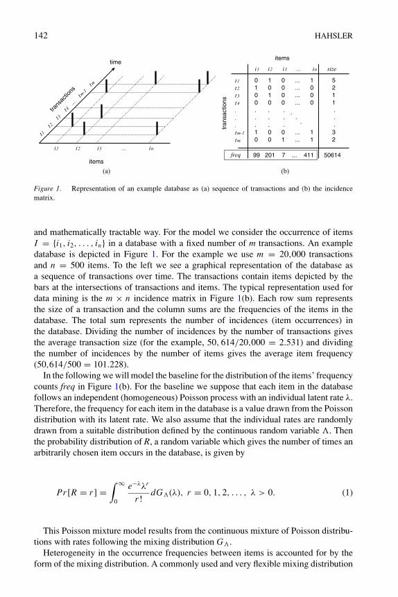
where n is the number of available items. In Figure 2 we show for the data sets thenumber of frequent 1-itemsets predicted by the fitted models (solid line) and the actualnumber (dashed line) by a varying minimum support constraint. For easier comparisonwe show relative support for the plots. In all three plots we can see how the models fitthe skewed support distributions.

3.3. Extending the baseline model to k-itemsets

After only considering 1-itemsets, we show how the model developed above can be ex-tended to provide a baseline for the distribution of support over all possible 1-extensionsof an itemset.

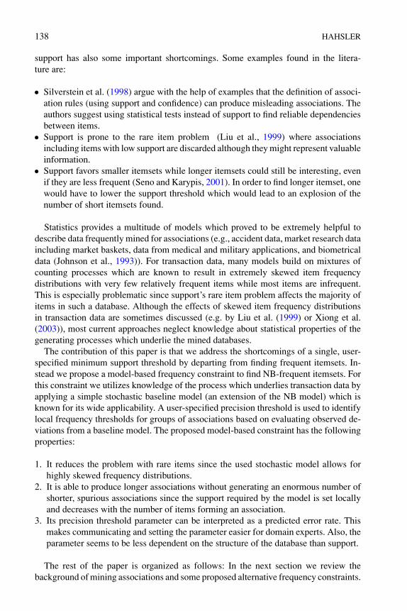
We start with 2-itemsets before we generalize to itemsets of arbitrary length.Figure 3 shows an example of the co-occurrence frequencies of all items (occurrenceof 2-itemsets) in transactions organized as an n × n matrix. The matrix is symmetricaround the main diagonal which contains the count frequencies of the individual itemsfreq(i1), freq(i2), . . . , freq(in). By adding the count values for each row or for each


0.000 0.005 0.010 0.015 0.020 0.025 0.030

050

100

150

200

250

300

Minimum support

Num

ber

of fr

eque

nt 1

–ite

mse

ts

WebView–1NB model

0.00 0.01 0.02 0.03 0.04 0.05

020

040

060

080

010

00

Minimum support

Num

ber

of fr

eque

nt 1

–ite

mse

ts

POSNB model

0.00 0.02 0.04 0.06 0.08 0.10

020

040

060

080

0

Minimum support

Num

ber

of fr

eque

nt 1

–ite

mse

ts

Artif–1NB model

Figure 2. Actual versus predicted number of frequent items by minimum support.

i1

items

i2

i3

in

...

i1 i2 i3 in...

99

32

32 0 12

201 3 134

0 3 7 6

40 134 6 411

item

s

211 599 37 2321

211

599

37

2321

...

...

...

...

...

... ... ... ... ...

Figure 3. A n × n matrix for counting 2-itemsets in the database.

column, we get in the margins of the matrix the number of incidences in all transactionswhich contain the respective item.

For example, to build the model for all 1-extensions of item i2, we only need theinformation in the box in Figure 3. It contains the frequency counts for all 1-extensionsof i2 plus freq(i2) in cell (2, 2). Note, that these counts are only affected by transactionswhich contain item i2. If we select all transactions which contain item i2, we get a sampleof size freq(i2) = 201 from the database. For the baseline model with only independentitems, the co-occurrence counts in the sample follow again Poisson processes. Following

148 HAHSLER

the model in Section 3.1 we canobtain a new random variable Ri2 which models theoccurrences of an arbitrarily chosen 1-extensions of i2.

After presenting the idea for the 1-extensions of a single item, we now turn tothe general case of building a baseline model for all 1-extensions of an associa-tion l of arbitrary length. We denote the number of items in l by k. Thus l is a k-itemset for which exactly n–k different 1-extensions exist. All 1-extensions of l canbe generated by joining l with all possible single items c ∈ I \ l. The items c willbe call candidate items. In the baseline model all candidate items are independentfrom the items in l. Consequently, the set of all transactions which contain l repre-sent a sample of size freq(l), which is random with respect to the candidate items.Following the developed model also the baseline for the number of candidate itemswith frequency r in the sample has a NB distribution. More precisely, the counts forthe 1-extensions of l can be modeled by a random variable Rl with the probabilitydistribution

Pr [Rl = r ] = (1 + al )−k �(k + r )

�(r + 1)�(k)

(al

1 + al

)r

for r = 0, 1, 2, . . . (5)

The distribution’s shape parameter k is not affected by sample size and we can usethe estimate k from the database. However, the parameter a is linearly dependent on thesample size (see Section 3.2 above). To obtain al , we have to rescale a, estimated fromthe database, for the sample size freq(l).

To rescale a we could use the proportion of the transactions in the sample relative tothe size of the database which was used to estimate a. In Section 3.2 above, we showedthat for estimating the parameter for different sample sizes gives a stable value for aper transaction. A problem with applying transaction-based rescaling is that the moreitems we include in l, the smaller the number of remaining items per transaction gets.This would reduce the effective transaction length and the estimated model would notbe applicable. Therefore, we will ignore the concept of transactions for the followingand treat the data set as a series of incidences (occurrences of items). For the baselinemodel this is unproblematic since the mixture model never used the information thatitems occur together in transactions. At the level of incidences, we can rescale a by theproportion of incidences in the sample relative to the total number of incidences in thedatabase from which we estimated the parameter. We do this in two steps:

1. We calculate a′, the parameter per incidence, by dividing the parameter obtainedfrom the database by the total number of incidences in the database.

a′ = a∑t∈D |t | (6)

2. We rescale the parameter for itemset l by multiplying a′ with the number of incidencesin the sample (transactions which contain l) excluding the occurrences of the itemsin l.

al = a′ ∑{t∈D|t⊃l}

|t \ l| (7)


For item i2 in the example in Figure 3, the rescaled parameter can be easily calculatedfrom the sum of incidences for the item (599) in the n × n matrix together with thethe sum of incidences (50,614) in the total incidence matrix (see Figure 1 above inSection 3.1) by a′ = a/50614 and ai2 = a′ · 599.

3.4. Deriving a model-based frequency constraint for NB-frequent itemsets

The NB distribution with the parameters rescaled for itemset l provides a baseline forthe frequency distribution of the candidate items in the transactions which contain l,i.e., the number of different itemsets l ∪ {c} with c ∈ I \ l we would expect per supportcount, if all items were independent. If in the database some item candidates are relatedto the items in l, the transactions that contain l cannot be considered a random samplefor these items. These related items will have a higher frequency in the sample thanexpected by the baseline model.

To find a set L of non-random 1-extensions of l (extensions with item candidates witha too high co-occurrence frequency), we need to identify a frequency threshold σ

freql ,

where accepting item candidates with a frequency count r ≥ σfreql separates associated

items best from items which co-occur often by pure chance. For this task we need todefine a quality measure on L, the set of accepted 1-extensions. Precision is a possiblequality measure which is widely used by the machine learning community (Kohavi andProvost, 1988) and is defined as the proportion of correctly predicted positive cases inall predicted positive cases. Using the baseline model and observed data, we can predictprecision for different values of the frequency threshold.

Definition 2 (Predicted precision). Let L be the set of all 1-extensions of a knownassociation l which are generated by joining l with all candidate items c ∈ I \ l whichco-occurrence with l in at least ρ transactions. For set L we define the predicted precisionas

precisionl(ρ) =(o[r≥ρ] − e[r≥ρ]

)/o[r≥ρ] if o[r≥ρ] ≥ e[r≥ρ] and o[r≥ρ] > 0

0 otherwise.(8)

o[r ≥ ρ] is the observed and e[r≥ρ] is the expected number of candidate items whichhave a co-occurrence frequency with itemset l of r ≥ ρ. The observed number iscalculated as the sum of observations with count r by o[r≥ρ] = ∑rmax

r=ρ or , where rmax

is the highest observed co-occurrence. The expected number is given by the baselinemodel as e[r≥ρ] = (n − |l|)Pr [Rl ≥ ρ], where n − |l| is the number of possiblecandidate items for pattern l.

Predicted precision together with a precision threshold π can be used to form a model-based constraint on accepted associations. The smallest possible frequency threshold for1-extensions of l, which satisfies the set minimum precision threshold π , can be foundby

σfreql = argminρ{precisionl(ρ) ≥ π}. (9)

150 HAHSLER

The set of the chosen candidate items for l is then

Cl = {c ∈ I \ l|freq(l ∪ {c}) ≥ σfreql },

and the set of accepted associations is

L = {l ∪ {c}|c ∈ Cl}.

The predicted error rate for using a threshold σfreql is given by 1 − precisionl(σ

freql ).

A suitable selection criterion for a count threshold is to allow only a percentage offalsely accepted associations. For example, if we need for an application all rules withthe antecedent l and a single item as the consequent and the maximum number ofacceptable spurious rules is 5%, we can find all 1-extension of l and use a minimumprecision threshold of π = 0.95.

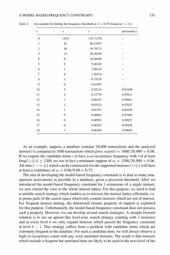
Table 4 contains an example for the model-based frequency constraint usingdata from the WebView-1 database. We analyze the 1-extensions of itemset l ={10311, 12571, 12575} at a minimum precision threshold of 95%. The estimates forn, k and a are taken from Table 2 in Section 3.2. Parameter a is rescaled to al = 1.164using Eqs. (6) and (7) in the previous section. Column o contains the observed numberof items with a co-occurrence frequency of r with l. The value at r = 0 is in parenthe-ses since it is not directly observable. It was calculated as the difference between theestimated number of available candidate items (n − |l|) and the number of observeditems (o[r > 0]). Column e contains the expected frequencies calculated with the model.To find the frequency threshold σ

freql , the precision function precisionl (ρ) in Eq. (8) is

evaluated starting with ρ = rmax (18 in the example in Table 4) and ρ is reduced tillwe get a predicted precision value which is below the minimum precision threshold ofπ = 0.95. The found frequency threshold is then the last value for r, which produced aprecision above the threshold (in the example at r = 11). After the threshold is found,there is no need to evaluate the rest of the precision function with r < 10. All candidateitems with a co-occurrence frequency greater than the found threshold are selected. Forthe example in Table 4, this gives a set of 6 chosen candidate items.

There exists an interesting connection to the confidence measure for the way anindividual frequency threshold (minimum support) is chosen for all 1-extensions of anitemset.

Theorem 1. Let l be an itemset and let c ∈ I \ l be the set of candidate items whichform together with l all 1-extensions of l. For each possible minimum support σl on the1-extensions of l, a minimum confidence threshold γl on the rules l −→ {c} exists, whichresults in an equivalent constraint. That is, there always exist pairs of values for σl andγl were the following holds:

supp(l ∪ {c}) ≥ σl ⇔ conf(l −→ {c}) ≥ γl .

Proof 1 With conf(l −→ {c}) defined as supp(l ∪ {c})/supp(l) we can rewrite theright-hand side constraint as supp(l ∪ {c})/supp(l) ≥ γl . Since supp(l) is a positiveconstant for all considered rules, we get the equality γl = σl/supp(l) by substitution.�


Table 4. An example for finding the frequency threshold at π = 0.95 (found at r = 11).

r o e precision(r)

0 (183) 176.71178 –

1 81 80.21957 –

2 48 39.78173 –

3 13 20.28450 –

4 6 10.48480 –

5 0 5.46345 –

6 1 2.86219 –

7 0 1.50516 –

8 1 0.79378 –

9 0 0.41955 –

10 0 0.22214 0.92108

11 2 0.11779 0.95811

12 1 0.06253 0.96661

13 1 0.03323 0.97632

14 1 0.01767 0.98109

15 0 0.00941 0.97986

16 0 0.00501 0.98927

17 0 0.00267 0.99428

18 1 0.00305 0.99695

As an example, suppose a database contains 20,000 transactions and the analyzeditemset l is contained in 1600 transactions which gives supp(l) = 1600/20,000 = 0.08.If we require the candidate items c to have a co-occurrence frequency with l of at leastfreq(l ∪ {c}) ≥ 1200, we use in fact a minimum support of σl = 1200/20,000 = 0.06.All rules l −→ {c} which can be constructed for the supported itemsets l ∪{c} will haveat least a confidence of γl = 0.06/0.08 = 0.75.

The aim of developing the model-based frequency constraint is to find as many non-spurious associations as possible in a database, given a precision threshold. After weintroduced the model-based frequency constraint for 1-extensions of a single itemset,we now extend the view to the whole itemset lattice. For this purpose, we need to finda suitable search strategy which enables us to traverse the itemset lattice efficiently, i.e.to prune parts of the search space which only contain itemsets which are not of interest.For frequent itemset mining, the downward closure property of support is exploitedfor this purpose. Unfortunately, the model-based frequency constraint does not possesssuch a property. However, we can develop several search strategies. A straight forwardsolution is to use an apriori-like level-wise search strategy (starting with 1-itemsets)and in every level k we only expand itemsets which passed the frequency constraintat level k − 1. This strategy suffers from a problem with candidate items which areextremely frequent in the database. For such a candidate item, we will always observe ahigh co-occurrence count with any, even unrelated itemsets. The result is that itemsetswhich include a frequent but unrelated item are likely to be used in the next level of the

152 HAHSLER

algorithm and possibly will be expanded even further. In transaction databases with avery skewed item frequency distribution this leads to many spurious associations andcombinatorial explosion.

Alternatively, since each k-itemset can be produced from k different (k − 1)-subsets(checked at level k − 1) plus the corresponding candidate item, it is also possible torequire that for all (k−1)-subsets the corresponding candidate item passes the frequencyconstraint. This strategy makes intuitively sense since for associated items one expectsthat each item in the set is associated with the rest of the itemsets and thus shouldpass the constraint. It also solves the problem with extremely frequent candidate itemssince it is very unlikely that all unrelated and less frequent items pass by chance thepotentially high frequency constraint for the extremely frequent item. Furthermore, thisstrategy prunes the search space significantly since an itemset is only used for expansionif all subsets passed the frequency constraint. However, the strategy has a problem withincluding a relatively infrequent item into a set consisting of more frequent items. It isless likely that the infrequent item as the candidate item meets the frequency constraintset by the more frequent itemset, even if it is related. Therefore it is possible that itemsetsconsisting of related items with varying frequencies are missed.

A third solution is to used a trade-off between the problems and pruning effects of thetwo search strategies by requiring for a fraction θ (between one and all) of the subsetswith their candidate items to pass the frequency constraint. We now formally introducethe concept of NB-frequent itemsets which can be used to implement all three solutions:

Definition 3 (NB-frequent itemset). A k-itemset l ′ with k > 1 is a NB-frequentitemset if, and only if, at least a fraction θ (at least one) of its (k − 1)-subsets l ∈{l ′ \ {c}|c ∈ l ′} are NB-frequent itemsets and satisfy freq(l ∪{c}) ≥ σ

freql . The frequency

thresholds σfreql are individually chosen for each itemset l using Eq. (9) with a user-

specified precision threshold π . All itemsets of size 1 are per definition NB-frequent.

This definition clearly shows that NB-frequency in general is not downward closedsince only a fraction θ of the (k − 1)-subsets of a NB-frequent set of size k are requiredto be also NB-frequent. Only the special case with θ = 1 offers downward closure, butsince the definition of NB-frequency is recursive, we can only determine if an itemsetis NB-frequent if we first evaluate all its subsets. However, the definition enables us tobuild algorithms which find all NB-frequent itemsets in a bottom-up search (expandingfrom 1-itemsets) and even to prune the search space. The magnitude of pruning dependson the setting for parameter θ .

Conceptually, mining NB-frequent itemsets with the extreme values 0 and 1 for θ issimilar to using Omiecinski’s (2003) any-confidence and all-confidence. In Theorem 1we showed that the minimum support σl chosen for NB-frequent itemsets l ∪ {c} isequivalent to choosing a minimum on confidence γl = σl/supp(l) for the rules l −→ {c}.An itemset passes a threshold on any-confidence if at least one rule can be constructedfrom the itemset which has a confidence value greater or equal of the threshold. This issimilar to mining NB-frequent itemsets with θ = 0, where to accept itemset l ∪ {c} asingle combination conf(l −→ {c}) ≥ γl suffices.

For all-confidence, all rules which can be constructed from an itemset must havea confidence greater or equal than a threshold. This is similar to mining NB-frequentitemsets with θ = 1 where we require conf(l −→ {c}) ≥ γl for all possible combination.


Note, that in contrast to all- and any-confidence, we do not use a single threshold formining NB-frequent itemsets, but an individual threshold is chosen by the model for eachitemset l.

4. A mining algorithm for NB-frequent itemsets

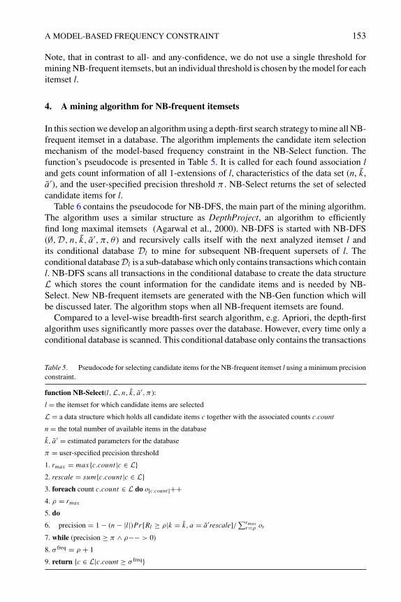
In this section we develop an algorithm using a depth-first search strategy to mine all NB-frequent itemset in a database. The algorithm implements the candidate item selectionmechanism of the model-based frequency constraint in the NB-Select function. Thefunction’s pseudocode is presented in Table 5. It is called for each found association land gets count information of all 1-extensions of l, characteristics of the data set (n, k,a′), and the user-specified precision threshold π . NB-Select returns the set of selectedcandidate items for l.

Table 6 contains the pseudocode for NB-DFS, the main part of the mining algorithm.The algorithm uses a similar structure as DepthProject, an algorithm to efficientlyfind long maximal itemsets (Agarwal et al., 2000). NB-DFS is started with NB-DFS(∅,D, n, k, a′, π, θ ) and recursively calls itself with the next analyzed itemset l andits conditional database Dl to mine for subsequent NB-frequent supersets of l. Theconditional databaseDl is a sub-database which only contains transactions which containl. NB-DFS scans all transactions in the conditional database to create the data structureL which stores the count information for the candidate items and is needed by NB-Select. New NB-frequent itemsets are generated with the NB-Gen function which willbe discussed later. The algorithm stops when all NB-frequent itemsets are found.

Compared to a level-wise breadth-first search algorithm, e.g. Apriori, the depth-firstalgorithm uses significantly more passes over the database. However, every time only aconditional database is scanned. This conditional database only contains the transactions

Table 5. Pseudocode for selecting candidate items for the NB-frequent itemset l using a minimum precisionconstraint.

function NB-Select(l,L, n, k, a′, π ):

l = the itemset for which candidate items are selected

L = a data structure which holds all candidate items c together with the associated counts c.count

n = the total number of available items in the database

k, a′ = estimated parameters for the database

π = user-specified precision threshold

1. rmax = max{c.count |c ∈ L}2. rescale = sum{c.count |c ∈ L}3. foreach count c.count ∈ L do o[c.count]++4. ρ = rmax

5. do

6. precision = 1 − (n − |l|)Pr [Rl ≥ ρ|k = k, a = a′rescale]/∑rmax

r=ρ or

7. while (precision ≥ π ∧ ρ−− > 0)

8. σ freq = ρ + 1

9. return {c ∈ L|c.count ≥ σ freq}

154 HAHSLER

Table 6. Pseudocode for a recursive depth-first search algorithm for NB-frequent itemsets.

algorithm NB-DFS (l,Dl , n, k, a′, π, θ ):

l = a NB-frequent itemset

Dl = a conditional database only containing transactions which include l

n = the number of all available items in the database

k, a′ = estimated parameters for the database

π = user-specified precision threshold

θ = user-specified required fraction of NB-frequent subsets

L = data structure for co-occurrence counts

1. L = ∅2. foreach transaction t ∈ Dl do begin

3. foreach candidate item c ∈ t \ l do begin

4. if c ∈ L then c.count++

5. else add new counter c.count = 1 to L6. end

7. end

8. if l �= ∅ then selected candidates C = NB-Select (l,L, n, k, a′, π )

9. else initial run candidates are C = {c ∈ L}10. delete or save data structure L11. L = NB − Gen(l, C, θ )

12. foreach new NB-frequent itemset l ′ ∈ L do begin

13. Dl ′ = {t ∈ Dl |t ⊇ l ′}14. L = L ∪ NB-DFS(l ′,Dl ′ , n, k, a′, π, θ )

15. end

16. return L

that include the itemset which is currently expanded. Note, that this conditional databasecontains all information needed to find all NB-frequent supersets of the expandeditemset. As this itemset grows longer, the conditional database gets quickly smaller. Ifthe original database is too large to fit into main memory, a conditional databases will fitinto the memory after the expanded itemset grew in size. This will make the subsequentscans very fast.

The generation function NB-Gen has a similar purpose as candidate generation insupport-based algorithms: It controls what parts of the search space are pruned. There-fore, a suitable candidate generation strategy is crucial for the performance of the miningalgorithm. As already discussed, NB-frequency does not possess the downward closureproperty which would allow pruning in the same way as for minimum support. However,the definition of NB-frequent itemsets provides us with a way to prune the search space.From the definition we know that in order for a k-itemset to be NB-frequent at leasta proportion θ of its (k − 1)-subset have to be NB-frequent and produce the itemsettogether with an accepted candidate item. Since for each k-itemset exist k differentsubsets of size k − 1, we only need to continue the depth-first search for the k-itemset,


Table 7. Pseudocode for the generation function for NB-frequent itemsets.

function NB-Gen (l, C, θ ))

l = a NB-frequent itemset

C = the set of candidate items chosen by NB-Select for l

θ = a user-specified parameter

R = a global repository containing for each traversed itemset l′ of size k an entry l′.frequent which is trueif l′ was already determined to be NB-frequent, and a counter l′.count to keep track of the number ofNB-frequent (k − 1)-subsets for which l′ was already accepted as a candidate.

1. L = {l ∪ {c}|c ∈ C}2. foreach candidate itemset l ′ ∈ L do begin

3. if l ′ /∈ R then add l′ with l′.frequent = false and l ′.count = 0 to R4. if l ′.frequent == true then delete l′ from L

5. else begin

6. l ′.count++7. if l ′.count < θ |l ′| then delete l′ from L

8. else l ′. frequent = true

9. end

10. end

11. return L

for which we already found at least kθ NB-frequent (k − 1)-subset. This has a pruningeffect on the search space size.

We present the pseudocode for the generation functions in Table 7. The function iscalled for each found NB-frequent itemset l individually and gets the set of acceptedcandidate items and the parameter θ . To enforce θ for the generation of a new NB-frequent itemset l ′ of size k, we need the information of how many different NB-frequentsubsets of size k − 1 also produce l ′. And, at the same time, we need to make sure thatno part of the lattice is traversed more than once. Other depth-first mining algorithms(e.g., FP-Growth or DepthProject) solve this problem by using special representationsof the database (frequent pattern tree structures (Han et al., 2004) or a lexicographictree (Agarwal et al., 2000)). These representations ensure that no part of the searchspace can be traversed more than once. However, these techniques only work for frequentitemsets using the downward closed minimum support constraint. To enforce the fractionθ for NB-frequent itemsets and to ensure that itemsets in the lattice are only traversedonce by NB-DFS, we use a global repository R. This repository is used to keep track ofthe number of times a candidate itemset was already generated and of the itemsets whichwere already traversed. This solution was inspired by the implementation of closed andmaximal itemset filtering implemented for the Eclat algorithm by Borgelt (2003).

5. Experimental results

In this section we analyze the properties and the effectiveness of mining NB-frequentitemsets. To compare the performance of NB-frequent itemsets with existing methodswe use frequent itemsets and itemsets generated using all-confidence as benchmarks. We

156 HAHSLER

chose frequent itemsets since a single support value represents the standard in miningassociation rules. All-confidence was chosen because of its promising properties and itsconceptual similarity with mining NB-frequent itemsets with θ = 1.

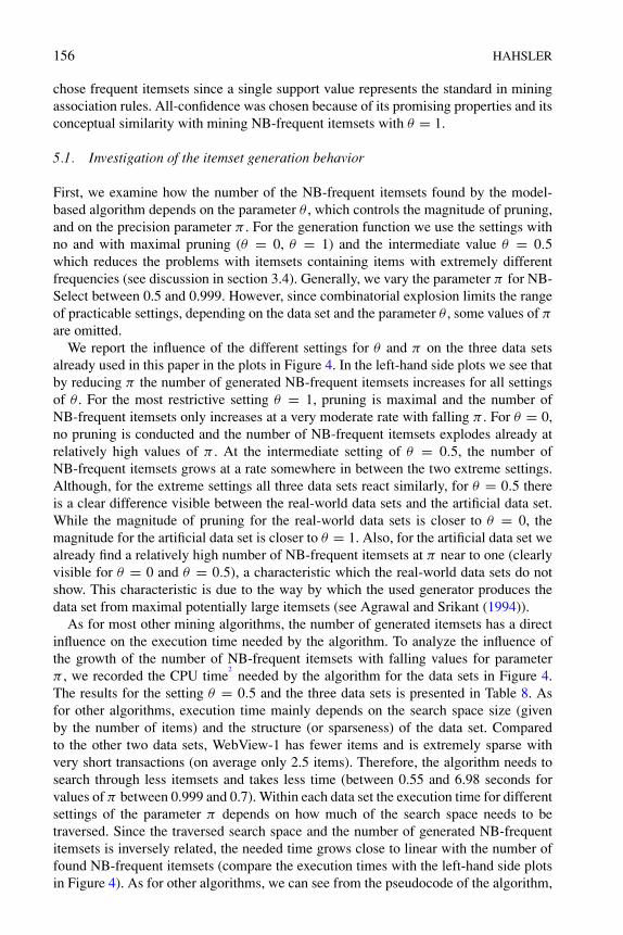
5.1. Investigation of the itemset generation behavior

First, we examine how the number of the NB-frequent itemsets found by the model-based algorithm depends on the parameter θ , which controls the magnitude of pruning,and on the precision parameter π . For the generation function we use the settings withno and with maximal pruning (θ = 0, θ = 1) and the intermediate value θ = 0.5which reduces the problems with itemsets containing items with extremely differentfrequencies (see discussion in section 3.4). Generally, we vary the parameter π for NB-Select between 0.5 and 0.999. However, since combinatorial explosion limits the rangeof practicable settings, depending on the data set and the parameter θ , some values of π

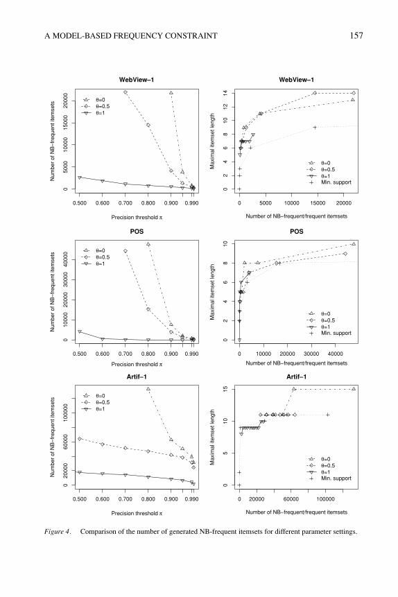
are omitted.We report the influence of the different settings for θ and π on the three data sets

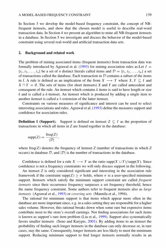
already used in this paper in the plots in Figure 4. In the left-hand side plots we see thatby reducing π the number of generated NB-frequent itemsets increases for all settingsof θ . For the most restrictive setting θ = 1, pruning is maximal and the number ofNB-frequent itemsets only increases at a very moderate rate with falling π . For θ = 0,no pruning is conducted and the number of NB-frequent itemsets explodes already atrelatively high values of π . At the intermediate setting of θ = 0.5, the number ofNB-frequent itemsets grows at a rate somewhere in between the two extreme settings.Although, for the extreme settings all three data sets react similarly, for θ = 0.5 thereis a clear difference visible between the real-world data sets and the artificial data set.While the magnitude of pruning for the real-world data sets is closer to θ = 0, themagnitude for the artificial data set is closer to θ = 1. Also, for the artificial data set wealready find a relatively high number of NB-frequent itemsets at π near to one (clearlyvisible for θ = 0 and θ = 0.5), a characteristic which the real-world data sets do notshow. This characteristic is due to the way by which the used generator produces thedata set from maximal potentially large itemsets (see Agrawal and Srikant (1994)).

As for most other mining algorithms, the number of generated itemsets has a directinfluence on the execution time needed by the algorithm. To analyze the influence ofthe growth of the number of NB-frequent itemsets with falling values for parameterπ , we recorded the CPU time

2needed by the algorithm for the data sets in Figure 4.

The results for the setting θ = 0.5 and the three data sets is presented in Table 8. Asfor other algorithms, execution time mainly depends on the search space size (givenby the number of items) and the structure (or sparseness) of the data set. Comparedto the other two data sets, WebView-1 has fewer items and is extremely sparse withvery short transactions (on average only 2.5 items). Therefore, the algorithm needs tosearch through less itemsets and takes less time (between 0.55 and 6.98 seconds forvalues of π between 0.999 and 0.7). Within each data set the execution time for differentsettings of the parameter π depends on how much of the search space needs to betraversed. Since the traversed search space and the number of generated NB-frequentitemsets is inversely related, the needed time grows close to linear with the number offound NB-frequent itemsets (compare the execution times with the left-hand side plotsin Figure 4). As for other algorithms, we can see from the pseudocode of the algorithm,


WebView–1

Precision threshold π

Num

ber

of N

B–

freq

uent

item

sets

0.500 0.600 0.700 0.800 0.900 0.990

050

0010

000

1500

020

000

θ=0θ=0.5θ=1

0 5000 10000 15000 20000

02

46

810

1214

WebView–1

Number of NB–frequent/frequent itemsetsM

axim

al it

emse

t len

gth

θ=0θ=0.5θ=1Min. support

POS


Num

ber

of N

B–

freq

uent

item

sets

0.500 0.600 0.700 0.800 0.900 0.990

010

000

2000

030

000

4000

0 θ=0θ=0.5θ=1

0 10000 20000 30000 40000

02

46

810

POS

Number of NB– frequent/frequent itemsets

Max

imal

item

set l

engt

h


Artif–1


Num

ber

of N

B–

freq

uent

item

sets

0.500 0.600 0.700 0.800 0.900 0.990

020

000

6000

010

0000

θ=0θ=0.5θ=1

0 20000 60000 100000

05

1015

Artif–1

Number of NB–frequent/frequent itemsets

Max

imal

item

set l

engt

h


Figure 4. Comparison of the number of generated NB-frequent itemsets for different parameter settings.

158 HAHSLER

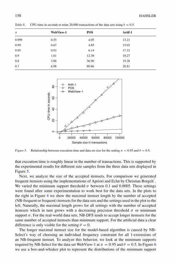
Table 8. CPU-time in seconds to mine 20,000 transactions of the data sets using θ = 0.5.

π WebView-1 POS Artif-1

0.999 0.55 4.05 13.21

0.99 0.67 4.85 15.03

0.95 0.92 6.14 17.32

0.9 1.61 12.38 18.27

0.8 3.88 36.90 19.28

0.7 6.98 80.66 20.81

Sample size in transactions

CP

U–

time

in s

econ

ds

020

4060

80

0 20000 40000 60000 80000 100000

Artif–1POSWebView–1

Figure 5. Relationship between execution time and data set size for the setting π = 0.95 and θ = 0.5.

that execution time is roughly linear in the number of transactions. This is supported bythe experimental results for different size samples from the three data sets displayed inFigure 5.

Next, we analyze the size of the accepted itemsets. For comparison we generatedfrequent itemsets using the implementations of Apriori and Eclat by Christian Borgelt

3.

We varied the minimum support threshold σ between 0.1 and 0.0005. These settingswere found after some experimentation to work best for the data sets. In the plots tothe right in Figure 4 we show the maximal itemset length by the number of accepted(NB-frequent or frequent) itemsets for the data sets and the settings used in the plot to theleft. Naturally, the maximal length grows for all settings with the number of accepteditemsets which in turn grows with a decreasing precision threshold π or minimumsupport σ . For the real-world data sets, NB-DFS tends to accept longer itemsets for thesame number of accepted itemsets than minimum support. For the artificial data a cleardifference is only visible for the setting θ = 0.

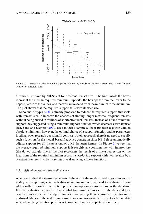
The longer maximal itemset size for the model-based algorithm is caused by NB-Select’s way of choosing an individual frequency constraint for all 1-extensions ofan NB-frequent itemset. To analyze this behavior, we look at the minimum supportsrequired by NB-Select for the data set WebView-1 at π = 0.95 and θ = 0.5. In Figure 6we use a box-and-whisker plot to represent the distributions of the minimum support


2 3 4 5 6 7 8 9

0.00

10.

003

0.00

7

WebView–1, π=0.95, θ=0.5

Itemset size

Req

uire

d m

in. s

uppo

rt (

log)

0.00

015

Regression line

Figure 6. Boxplot of the minimum support required by NB-Select forthe 1-extensions of NB-frequentitemsets of different size.

thresholds required by NB-Select for different itemset sizes. The lines inside the boxesrepresent the median required minimum supports, the box spans from the lower to theupper quartile of the values, and the whiskers extend from the minimum to the maximum.The plot shows that the required support falls with itemset size.

Seno and Karypis (2001) already proposed to reduce the required support thresholdwith itemset size to improve the chances of finding longer maximal frequent itemsetswithout being buried in millions of shorter frequent itemsets. Instead of a fixed minimumsupport they suggested using a minimum support function which decreases with itemsetsize. Seno and Karypis (2001) used in their example a linear function together with anabsolute minimum, however, the optimal choice of a support function and its parametersis still an open research question. In contrast to their approach, there is no need to specifysuch a function for the model-based frequency constraint since NB-Select automaticallyadjusts support for all 1-extensions of a NB-frequent itemset. In Figure 6 we see thatthe average required minimum support falls roughly at a constant rate with itemset size(the dotted straight line in the plot represents the result of a linear regression on thelogarithm of the required minimum supports). Reducing support with itemset size by aconstant rate seems to be more intuitive than using a linear function.

5.2. Effectiveness of pattern discovery

After we studied the itemset generation behavior of the model-based algorithm and itsability to accept longer itemsets than minimum support, we need to evaluate if theseadditionally discovered itemsets represent non-spurious associations in the database.For the evaluation we need to know what true associations exist in the data and thencompare how effective the algorithm is in discovering these itemsets. Since for mostreal-world data sets the underlying associations are unknown, we resort to artificial datasets, where the generation process is known and can be completely controlled.

160 HAHSLER

To generate artificial data sets we use the popular generator developed by Agrawaland Srikant (1994). To evaluate the effectiveness of association discovery, we need toknow all associations which were used to generate the data set. In the original version ofthe generator only the associations with the highest occurrence probability are reported.Therefore, we adapted the code of the generator so that all used associations (calledmaximal potentially large itemsets) are reported. We generated two artificial data setsusing this modified generator. Both data sets consist of |D| = 100,000 transactions, theaverage transaction size is |T | = 10, the number of items is N = 1,000, and for thecorrelation and corruption levels we use the default values (0.5 for both).

The first data set, Artif-1, represents the standard data set T10I4D100K presentedby Agrawal and Srikant (1994) and which is used for evaluation in many papers. Forthis data set |L| = 2,000 maximal potentially large itemsets with an average size of|I | = 4 are used.

For the second data set, Artif-2, we decrease the average association size to |I | = 2.This will produce more maximal potentially large itemsets of size one. These 1-itemsetsare not useful associations since they do not provide information about dependenciesbetween items. They can be considered noise in the generated database and, therefore,make finding longer associations more difficult. A side effect of reducing the averageassociation size is that the chance of using longer maximal potentially large itemsets forthe database generation is reduced. To work against this effect, we double their number to|L| = 4,000.

For the experiments, we use for both data sets the first 20,000 transactions for miningassociations. To analyze how the effectiveness is influenced by the data set size, we alsoreport results for sizes 5,000 and 80,000 for Artif-2. For the model-based algorithm weestimated the parameters of the model from the data sets and then mined NB-frequentitemsets with the settings 0, 0.5 and 1 for θ . For each of the three settings for θ , wevaried the parameter π between 0.999 and 0.1 (0.999, 0.99, 0.95, 0.9, 0.8 and in 0.1 stepsdown to 0.1). Because of combinatorial explosion discussed in the previous section, weonly used π ≥ 0.5 for θ = 0.5 and π ≥ 0.8 for θ = 0.

For comparison with existing methods we mined frequent itemsets at minimumsupport levels between 0.1 and 0.0005 (0.01, 0.005, 0.004, 0.003, 0.002, 0.0015, 0.0013,0.001, 0.0007, and 0.0005). And as a second benchmark we generated itemsets usingall-confidence. We varied the threshold on all-confidence between 0.01 and 0.6 (0.6,0.5, 0.4, 0.3, 0.2, 0.1, 0.05, 0.04, 0.03, 0.02, 0.01). The used minimum support levelsand all-confidence thresholds were found after some experimentation to cover a widearea of the possible true positives/false positives combinations for the data sets.

To compare the ability to discover associations which were used to generate theartificial data sets, we counted the true positives (itemsets and their subsets discoveredby the algorithm which were used in the data set generation process) and false positives(mined itemsets which were not used in the data set generation process). This informationtogether with the total number of all positives in the database (all itemsets used togenerate a data set) is used to calculate precision (the ratio of the number of truepositives by the number of all instances classified as positives) and recall (the ratio ofthe number of true positives by the total number of positives in the data). Precision/recallplots, a common evaluation tool in information retrieval and machine learning, are thenused to visually inspect the algorithms’ effectiveness over their parameter spaces.


0.0 0.2 0.4 0.6 0.8 1.0

0.0

0.2

0.4

0.6

0.8

1.0

Artif–1, 20000 trans.

Recall

Pre

cisi

on

θ=0θ=0.5θ=1Min. SupportAll–confidence

0.0 0.2 0.4 0.6 0.8 1.0

0.0

0.2

0.4

0.6

0.8

1.0


Recall

Pre

cisi

on


0.0 0.2 0.4 0.6 0.8 1.0

0.0

0.2

0.4

0.6

0.8

1.0


Recall

Pre

cisi

on


0.0 0.2 0.4 0.6 0.8 1.0

0.0

0.2

0.4

0.6

0.8

1.0


Recall

Pre

cisi

on


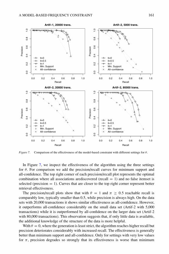
Figure 7. Comparison of the effectiveness of the model-based constraint with different settings for θ .

In Figure 7, we inspect the effectiveness of the algorithm using the three settingsfor θ . For comparison we add the precision/recall curves for minimum support andall-confidence. The top right corner of each precision/recall plot represents the optimalcombination where all associations arediscovered (recall = 1) and no false itemset isselected (precision = 1). Curves that are closer to the top right corner represent betterretrieval effectiveness.

The precision/recall plots show that with θ = 1 and π ≥ 0.5 reachable recall iscomparably low, typically smaller than 0.5, while precision is always high. On the datasets with 20,000 transactions it shows similar effectiveness as all-confidence. However,it outperforms all-confidence considerably on the small data set (Artif-2 with 5,000transactions) while it is outperformed by all-confidence on the larger data set (Artif-2with 80,000 transactions). This observation suggests that, if only little data is available,the additional knowledge of the structure of the data is more helpful.

With θ = 0, where the generation is least strict, the algorithm reaches higher recall butprecision deteriorates considerably with increased recall. The effectiveness is generallybetter than minimum support and all-confidence. Only for settings with very low valuesfor π , precision degrades so strongly that its effectiveness is worse than minimum

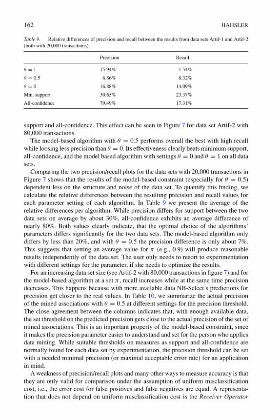
162 HAHSLER

Table 9. Relative differences of precision and recall between the results from data sets Artif-1 and Artif-2(both with 20,000 transactions).

Precision Recall

θ = 1 15.94% 1.54%

θ = 0.5 6.86% 8.32%

θ = 0 16.88% 14.09%

Min. support 30.65% 23.37%

All-confidence 79.49% 17.31%

support and all-confidence. This effect can be seen in Figure 7 for data set Artif-2 with80,000 transactions.

The model-based algorithm with θ = 0.5 performs overall the best with high recallwhile loosing less precision than θ = 0. Its effectiveness clearly beats minimum support,all-confidence, and the model based algorithm with settings θ = 0 and θ = 1 on all datasets.

Comparing the two precision/recall plots for the data sets with 20,000 transactions inFigure 7 shows that the results of the model-based constraint (especially for θ = 0.5)dependent less on the structure and noise of the data set. To quantify this finding, wecalculate the relative differences between the resulting precision and recall values foreach parameter setting of each algorithm. In Table 9 we present the average of therelative differences per algorithm. While precision differs for support between the twodata sets on average by about 30%, all-confidence exhibits an average difference ofnearly 80%. Both values clearly indicate, that the optimal choice of the algorithms’parameters differs significantly for the two data sets. The model-based algorithm onlydiffers by less than 20%, and with θ = 0.5 the precision difference is only about 7%.This suggests that setting an average value for π (e.g., 0.9) will produce reasonableresults independently of the data set. The user only needs to resort to experimentationwith different settings for the parameter, if she needs to optimize the results.

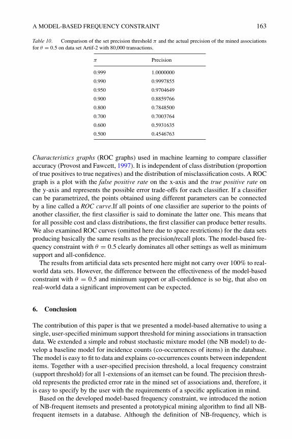
For an increasing data set size (see Artif-2 with 80,000 transactions in figure 7) and forthe model-based algorithm at a set π , recall increases while at the same time precisiondecreases. This happens because with more available data NB-Select’s predictions forprecision get closer to the real values. In Table 10, we summarize the actual precisionof the mined associations with θ = 0.5 at different settings for the precision threshold.The close agreement between the columns indicates that, with enough available data,the set threshold on the predicted precision gets close to the actual precision of the set ofmined associations. This is an important property of the model-based constraint, sinceit makes the precision parameter easier to understand and set for the person who appliesdata mining. While suitable thresholds on measures as support and all-confidence arenormally found for each data set by experimentation, the precision threshold can be setwith a needed minimal precision (or maximal acceptable error rate) for an applicationin mind.

A weakness of precision/recall plots and many other ways to measure accuracy is thatthey are only valid for comparison under the assumption of uniform misclassificationcost, i.e., the error cost for false positives and false negatives are equal. A representa-tion that does not depend on uniform misclassification cost is the Receiver Operator


Table 10. Comparison of the set precision threshold π and the actual precision of the mined associationsfor θ = 0.5 on data set Artif-2 with 80,000 transactions.

π Precision

0.999 1.0000000

0.990 0.9997855

0.950 0.9704649

0.900 0.8859766

0.800 0.7848500

0.700 0.7003764

0.600 0.5931635

0.500 0.4546763

Characteristics graphs (ROC graphs) used in machine learning to compare classifieraccuracy (Provost and Fawcett, 1997). It is independent of class distribution (proportionof true positives to true negatives) and the distribution of misclassification costs. A ROCgraph is a plot with the false positive rate on the x-axis and the true positive rate onthe y-axis and represents the possible error trade-offs for each classifier. If a classifiercan be parametrized, the points obtained using different parameters can be connectedby a line called a ROC curve.If all points of one classifier are superior to the points ofanother classifier, the first classifier is said to dominate the latter one. This means thatfor all possible cost and class distributions, the first classifier can produce better results.We also examined ROC curves (omitted here due to space restrictions) for the data setsproducing basically the same results as the precision/recall plots. The model-based fre-quency constraint with θ = 0.5 clearly dominates all other settings as well as minimumsupport and all-confidence.

The results from artificial data sets presented here might not carry over 100% to real-world data sets. However, the difference between the effectiveness of the model-basedconstraint with θ = 0.5 and minimum support or all-confidence is so big, that also onreal-world data a significant improvement can be expected.

6. Conclusion

The contribution of this paper is that we presented a model-based alternative to using asingle, user-specified minimum support threshold for mining associations in transactiondata. We extended a simple and robust stochastic mixture model (the NB model) to de-velop a baseline model for incidence counts (co-occurrences of items) in the database.The model is easy to fit to data and explains co-occurrences counts between independentitems. Together with a user-specified precision threshold, a local frequency constraint(support threshold) for all 1-extensions of an itemset can be found. The precision thresh-old represents the predicted error rate in the mined set of associations and, therefore, itis easy to specify by the user with the requirements of a specific application in mind.

Based on the developed model-based frequency constraint, we introduced the notionof NB-frequent itemsets and presented a prototypical mining algorithm to find all NB-frequent itemsets in a database. Although the definition of NB-frequency, which is

164 HAHSLER

based on local frequency constraints, does not provide the important downward closureproperty of support, we showed how the search space can be adequately reduced tomake efficient mining possible.

Experiments showed that the model-based frequency constraint automatically reducesthe average needed frequency (support) with growing itemset size. Compared withminimum support it tends to be more selective for shorter itemsets while still acceptinglonger itemsets with lower support. This property reduces the problem of being buriedin a great number of short itemsets when using a relatively low threshold in order toalso find longer itemsets.

Further experiments on artificial data sets indicate that the model-based constraintis more effective in finding non-spurious associations. The largest improvements werefound for noisy data sets or when only a relatively small database is available. Theseexperiments also show that the precision parameter of the model-based algorithm de-pends less than support or any-confidence on the data set. This is a huge advantage andreduces the need for time-consuming experimentation with different parameter settingsfor each new data set.

Finally, it has to be noted that the model-based constraint developed in this paper canonly be used for databases which are generated by a process similar to the developedbaseline model. The developed baseline is a robust and reasonable model for mosttransaction data (e.g., point-of-sale data). For other types of data, different baselinemodels can be developed and can then be incorporated in mining algorithms followingthe outline of this paper.

Acknowledgments

The author wishes to thank Blue Martini Software for contributing the KDD Cup 2000data, Ramakrishnan Srikant from the IBM Almaden Research Center for making thecode for the synthetic transaction data generator available, and to Christian Borgelt forthe free implementations of Apriori and Eclat.

The author especially thanks Andreas Geyer-Schulz and Kurt Hornik for the longdiscussions on modeling transaction data and the anonymous referees for their valuablecomments.

Notes

1. Although the artificial data set in this paper and in Zheng et al. (2001) were produced using the same gen-erator (available at http://www.almaden.ibm.com/software/quest/Resources/), there are minimal variationsdue to differences in the used random number generator initialization.

2. We used a machine with two Intel Xeon processors (2.4 GHz) running Linux (Debian Sarge). The algorithmwas implemented in JAVA and compiled using the gnu ahead-of-time compiler gcj version 3.3.5. CPUtime was recorded using the time command and we report the sum of user and system time.

3. Available at http://fuzzy.cs.uni-magdeburg.de/∼borgelt/software.html

References

Agarwal, R.C., Aggarwal, C.C., and Prasad, V.V.V. 2000. Depth first generation of long patterns. In Proceedingsof the 6th ACM SIGKDD International Conference on Knowledge Discovery and Data Mining, pp. 108–118.


Agrawal, R., Imielinski, T., and Swami, A. 1993. Mining association rules between sets of items in largedatabases. In Proceedings of the ACM SIGMOD International Conference on Management of Data, Wash-ington, DC, pp. 207–216.

Agrawal, R. and Srikant, R. 1994. Fast algorithms for mining association rules in large databases. In Pro-ceedings of the 20th International Conference on Very Large Data Bases, J. B. Bocca, M. Jarke, C. Zaniolo(Eds.) Santiago, Chile, pp. 487–499.

Borgelt, C. 2003. Efficient implementations of apriori and eclat. In Proceedings of the IEEE ICDM Workshopon Frequent Itemset Mining Implementations, B. Goethals, M.J. Zaki (Eds.) Melbourne, FL, USA.

Brin, S., Motwani, R., Ullman, J.D., and Tsur, S. 1997. Dynamic itemset counting and implication rules formarket basket data. In Proceedings of the ACM SIGMOD International Conference on Management ofData, Tucson, Arizona, USA, pp. 255–264.

Creighton, C. and Hanash, S. 2003. Mining gene expression databases for association rules. Bioinformatics,19(1):79–86.

Dempster, A.P., Laird, N.M., and Rubin, D.B. 1977. Maximum likelihood from incomplete data via the EMalgorithm. Journal of the Royal Statistical Society, Series B (Methodological), 39:1–38.

DuMouchel, W. and Pregibon, D. 2001. Empirical bayes screening for multiitem associations. In Proceedingsof the 7th ACM SIGKDD Intentional Conference on Knowledge Discovery in Databases and Data Mining,F. Provost, R. Srikant (Eds.) ACM Press, pp. 67–76.

Geyer-Schulz, A., Hahsler, M., and Jahn, M. 2002. A customer purchase incidence model applied to rec-ommender systems. In WEBKDD 2001—Mining Log Data Across All Customer Touch Points, ThirdInternational Workshop, San Francisco, CA, USA, August 26, 2001, Revised Papers, Lecture Notes inComputer Science LNAI 2356, R. Kohavi, B. Masand, M. Spiliopoulou, J. Srivastava (Eds.) Springer-Verlag, pp. 25–47.

Geyer-Schulz, A., Hahsler, M., Neumann, A., and Thede, A. 2003. Behaviorbased recommender systemsas value-added services for scienti.c libraries. In Statistical Data Mining & Knowledge Discovery, H.Bozdogan, (Ed.) Chapman & Hall/CRC, pp. 433–454.

Han, J., Pei, J., Yin, Y., and Mao, R. 2004. Mining frequent patterns without candidate generation. DataMining and Knowledge Discovery, 8:53–87.

Johnson, N.L., Kotz, S., and Kemp, A.W. 1993. Univariate Discrete Distributions, 2nd edn. New York: JohnWiley & Sons.

Kohavi, R., Brodley, C., Frasca, B., Mason, L., and Zheng, Z. 2000. KDD-Cup 2000 organizers’ report:Peeling the onion. SIGKDD Explorations, 2(2):86–98.

Kohavi, R. and Provost, F. 1988. Glossary of terms. Machine Learning, 30(2–3):271–274.Liu, B., Hsu, W., and Ma, Y. 1999. Mining association rules with multiple minimum supports. In Proceedings

of the 5th ACM SIGKDD International Conference on Knowledge Discovery and Data Mining, pp. 337–341.

Luo, J. and Bridges, S. 2000. Mining fuzzy association rules and fuzzy frequency episodes for intrusiondetection. International Journal of Intelligent Systems, 15(8):687–703.

Mannila, H., Toivonen, H., and Verkamo, A.I. 1994. Efficient algorithms for discovering association rules.In AAAI Workshop on Knowledge Discovery in Databases, U.M. Fayyad, R. Uthurusamy (Eds.) Seattle,Washington: AAAI Press, pp. 181–192,

Omiecinski, E.R. 2003. Alternative interest measures for mining associations in databases. IEEE Transactionson Knowledge and Data Engineering, 15(1):57–69.

Pei, J., Han, J., and Lakshmanan, L.V. 2001. Mining frequent itemsets with convertible constraints. InProceedings of the 17th International Conference on Data Engineering, April 02–06, 2001, Heidelberg,Germany, pp. 433–442.

Provost, F. and Fawcett, T. 1997. Analysis and visualization of classi.er performance: Comparison underimprecise class and cost distributions. In Proceedings of the 3rd International Conference on KnowledgeDiscovery and Data Mining, Heckerman, D., Mannila, H., and Pregibon, D., editors, Newport Beach, CA:AAAI Press, pp. 43–48.

Seno, M. and Karypis, G. 2001. Lpminer: An algorithm for finding frequent itemsets using length decreas-ing support constraint. In Proceedings of the 2001 IEEE International Conference on Data Mining, 29November–2 December 2001, N. Cercone, T.Y. Lin, X. Wu (Eds.) San Jose, California, USA: IEEEComputer Society, pp. 505–512.

Silverstein, C., Brin, S., and Motwani, R. 1998. Beyond market baskets: Generalizing association rules todependence rules. Data Mining and Knowledge Discovery, 2:39–68.

166 HAHSLER

Srivastava, J., Cooley, R., Deshpande, M., and Tan, P.-N. 2000. Web usage mining: Discovery and applicationsof usage patterns from web data. SIGKDD Explorations, 1(2):12–23.

Xiong, H., Tan, P.-N., and Kumar, V. 2003. Mining strong affinity association patterns in data sets with skewedsupport distribution. In Proceedings of the IEEE International Conference on Data Mining, November 19–22, 2003, B. Goethals, M.J. Zaki (Eds.) Melbourne, Florida, pp. 387–394.

Zheng, Z., Kohavi, R., and Mason, L. 2001. Real world performance of association rule algorithms. InProceedings of the 7th ACM SIGKDD International Conference on Knowledge Discovery in Databasesand Data Mining, F. Provost, R. Srikant (Eds.) ACM Press, pp. 401–406.

Documents

A Model-Based Frequency Constraint for Mining …michael.hahsler.net/research/nbd_dami2005/NBD_print.pdf · Both rely only on the conﬁdence measure deﬁned for association rules