Technical Paper 3680

A Model-Based Approach for the Measurementof Eye Movements Using Image Processing

Kwangjae Sung, Ph.D. and Millard F. Reschke, Ph.D.

April 1997

Technical Paper 3680

A Model-Based Approach for the Measurement of EyeMovements Using Image Processing

Kwangjae Sung, Ph.D.Visiting Scientist, University Space Research Association

Millard F. Reschke, Ph.D.Lyndon B. Johnson Space Center

April 1997

ii

This publication is available from the Center for AeroSpace Information, 800 Elkridge Landing Road,Linthicum Heights, MD 21090-2934 (301) 621-0390

iii

Contents

Abstract . . . . . . . . . . . . . . . . . . . . . . . . . . . . . . . . . . . . . . . . . . . . . . . . . . . . . . . . . . . . . . . . . . . . . . . . . . . . . . . . . . . 1

1.0 Introduction............................................................................... 1

2.0 Disk-Fitting Algorithm ... . . . . . . . . . . . . . . . . . . . . . . . . . . . . . . . . . . . . . . . . . . . . . . . . . . . . . . . . . . . . . . . 52.1 Assumptions.............................................................................. 52.2 Derivation of Least Squares Fit . . . . . . . . . . . . . . . . . . . . . . . . . . . . . . . . . . . . . . . . . . . . . . . . . . . . . . . . 62.3 Maximum Search .. . . . . . . . . . . . . . . . . . . . . . . . . . . . . . . . . . . . . . . . . . . . . . . . . . . . . . . . . . . . . . . . . . . . . . . 72.3.1 Comparison Search Method .. . . . . . . . . . . . . . . . . . . . . . . . . . . . . . . . . . . . . . . . . . . . . . . . . . . . . . . . . . . 82.3.2 Look-Up Tables for Relative Pixel Coordinates . . . . . . . . . . . . . . . . . . . . . . . . . . . . . . . . . . . . . 122.3.3 Initial Parameter Vector .. . . . . . . . . . . . . . . . . . . . . . . . . . . . . . . . . . . . . . . . . . . . . . . . . . . . . . . . . . . . . . . . 132.4 Image Threshold .. . . . . . . . . . . . . . . . . . . . . . . . . . . . . . . . . . . . . . . . . . . . . . . . . . . . . . . . . . . . . . . . . . . . . . . . 142.5 Subpixel Interpolation.. . . . . . . . . . . . . . . . . . . . . . . . . . . . . . . . . . . . . . . . . . . . . . . . . . . . . . . . . . . . . . . . . . 152.6 Elliptic Appearance of Pupil . . . . . . . . . . . . . . . . . . . . . . . . . . . . . . . . . . . . . . . . . . . . . . . . . . . . . . . . . . . . 15

3.0 Performance Evaluation.. . . . . . . . . . . . . . . . . . . . . . . . . . . . . . . . . . . . . . . . . . . . . . . . . . . . . . . . . . . . . . . . 173.1 Effect of Random Image Noise .. . . . . . . . . . . . . . . . . . . . . . . . . . . . . . . . . . . . . . . . . . . . . . . . . . . . . . . 173.1.1 Method .. . . . . . . . . . . . . . . . . . . . . . . . . . . . . . . . . . . . . . . . . . . . . . . . . . . . . . . . . . . . . . . . . . . . . . . . . . . . . . . . . . . 173.1.1.1 Pupil Model............................................................................... 183.1.1.2 Random Noises and Blurring .. . . . . . . . . . . . . . . . . . . . . . . . . . . . . . . . . . . . . . . . . . . . . . . . . . . . . . . . . 183.1.1.3 Data Measurement .. . . . . . . . . . . . . . . . . . . . . . . . . . . . . . . . . . . . . . . . . . . . . . . . . . . . . . . . . . . . . . . . . . . . . . 193.1.2 Simulation Results. . . . . . . . . . . . . . . . . . . . . . . . . . . . . . . . . . . . . . . . . . . . . . . . . . . . . . . . . . . . . . . . . . . . . . . 203.2 Performance With Occlusions of the Pupil Area .. . . . . . . . . . . . . . . . . . . . . . . . . . . . . . . . . . . . 223.2.1 Effect of Droopy Eyelid on the Disk-Fitting Algorithm ... . . . . . . . . . . . . . . . . . . . . . . . . . . 223.2.2 Effect of Light Reflection on Disk-Fitting Algorithm................................ 273.2.3 Comparison of Centroid and Disk-Fitting Algorithms With Simulated Artifacts 30

4.0 Implementation and Examples.......................................................... 33

5.0 Conclusions .. . . . . . . . . . . . . . . . . . . . . . . . . . . . . . . . . . . . . . . . . . . . . . . . . . . . . . . . . . . . . . . . . . . . . . . . . . . . . 36

References .. . . . . . . . . . . . . . . . . . . . . . . . . . . . . . . . . . . . . . . . . . . . . . . . . . . . . . . . . . . . . . . . . . . . . . . . . . . . . . . 38

iv

Contents(continued)

Figures1 Artificial pupil images with corresponding NRE surface profiles in

two-dimensional eye position domain......................................................... 9

2 Comparison of two neighboring pupil candidates illustrates a common area S . . . . . . . . . . 11

3 Ratio of the size of areas required to compare two pupil candidates....................... 12

4 Iterations required to converge on optimal pupil model. . . . . . . . . . . . . . . . . . . . . . . . . . . . . . . . . . . . . 14

5 Optimal radius measured by the disk-fitting algorithm when the pupil is an ellipsewith the major radius of 130 .. . . . . . . . . . . . . . . . . . . . . . . . . . . . . . . . . . . . . . . . . . . . . . . . . . . . . . . . . . . . . . . . . . 17

6 Samples of artificially generated pupil images .. . . . . . . . . . . . . . . . . . . . . . . . . . . . . . . . . . . . . . . . . . . . . . 18

7 Artificial pupil images used in the simulation with their corresponding thresholdedbinary image...................................................................................... 20

8 The performances of the disk-fitting method and centroid method are compared........ 21

9 Models of a pupil with partial occlusion from a droopy eyelid............................. 24

10 Measurement errors for pupils with a partial occlusion from a droopy eyelid can bederived by examining the value of ox at the NRE maxima .. . . . . . . . . . . . . . . . . . . . . . . . . . . . . . . . 26

11 Model of pupil occluded by a light reflection centered on the pupil edge .. . . . . . . . . . . . . . . . 27

12 Measurement errors for pupils with a partial occlusion from a light reflection can bederived by examining the value of ox at the NRE maxima .. . . . . . . . . . . . . . . . . . . . . . . . . . . . . . . . 29

13 Artificial pupil images used in the simulation with their corresponding thresholdedbinary image...................................................................................... 31

14 Measurement errors from the disk-fitting algorithm and centroid algorithm during asimulation of horizontal sinusoidal eye movements .. . . . . . . . . . . . . . . . . . . . . . . . . . . . . . . . . . . . . . . . 32

15 Block diagram of the VDAC system .......................................................... 33

16 Snapshots of real video eye images .. . . . . . . . . . . . . . . . . . . . . . . . . . . . . . . . . . . . . . . . . . . . . . . . . . . . . . . . . . 35

17 Measurement chart for the eye images shown in Figure 15(a) . . . . . . . . . . . . . . . . . . . . . . . . . . . . . 35

18 Measurement chart for the eye images shown in Figure 15(b). . . . . . . . . . . . . . . . . . . . . . . . . . . . . 36

1

Abstract

This paper describes a video eye-tracking algorithm which searches for the best fit of the pupil

modeled as a circular disk. The algorithm is robust to common image artifacts such as the droopy

eyelids and light reflections while maintaining the measurement resolution available by the centroid

algorithm. The presented algorithm is used to derive the pupil size and center coordinates, and can

be combined with iris-tracking techniques to measure ocular torsion. A comparison search method

of pupil candidates using pixel coordinate reference lookup tables optimizes the processing

requirements for a least square fit of the circular disk model. This paper includes quantitative

analyses and simulation results for the resolution and the robustness of the algorithm. The

algorithm presented in this paper provides a platform for a noninvasive, multidimensional eye

measurement system which can be used for clinical and research applications requiring the precise

recording of eye movements in three-dimensional space.

1.0 Introduction

Several different measurement techniques have been utilized to study the reflexive and voluntary

control of eye movements, and these methods have had significant diagnostic value in tests of

visual, oculomotor, and vestibular function. However, a survey of the technical limitations and

artifacts inherent in the most commonly used measurement systems explains why most clinical and

research applications have been restricted to the horizontal plane [1, 2]. Recently, considerable

research has been conducted on the neural processes involved in the coding and control of eye

movements in three-dimensional (3D) space. For example, for the vestibular system to stabilize

gaze and ensure clear vision, there must be a spatial coordinate transformation between vestibular

and oculomotor 3-D reference frames to ensure that eye movements compensate for the head

movement stimulus [3]. Most natural visual and vestibular stimuli contain combinations of

transitional, rotational, and tilt components which elicit a different type of compensatory eye

movement. Clearly a multidimensional measurement system is required to adequately characterize

reflex pathways which are involved in the 3D control of eye movements. Indeed, patient data from

various otolith-ocular tests have already demonstrated the diagnostic potential of using a

measurement system with this capability [4].

2

Although the magnetic search coil technique is generally regarded as the most precise measure of

3D eye movements, there are several disadvantages with this method which will continue to limit

its usage with human patients. The scleral contact lens worn by the subject during this procedure

must fit tightly to limit slippage artifacts, and consequently have potential side effects that restrict

the available test time, such as increased intraocular pressure and degradation in visual acuity due

to corneal deformation [5-8]. In addition, the choice of material composition for the surround and

restraint equipment is often constrained to avoid magnetic field distortion artifacts.

Of the other measurement systems available, noninvasive video image recording appears to be the

most practical alternative for multidimensional eye movement analysis. Under proper illumination

which usually uses the infrared light spectrum, the iris image pattern is characterized by high

spatial frequency components of angular direction obtained from the iris muscle striations, whereas

the pupil area consists of a contiguous uniform dark area. Then, characteristics of the iris and

pupil patterns can be used to track horizontal and vertical eye movements, torsion angle and the

pupil radius. Recent advances in video and computer technologies have resolved many of the

image quality and data processing difficulties with this approach. Another practical advantage of

this approach is the ability to record eye images on videotape for later re-analysis. This option

eliminates the risk of failed measurements due to the poor performance of the eye tracking system.

However, a major disadvantage has been sensitivity to image noise and artifacts, and a limited data

sampling rate which is confined by the video frame rate. The problem of limited data sampling rate

could be overcome by using high-speed video even though it adds complexity to the system. The

sensitivity to the image quality is more inherent to the video eye tracking method, and is highly

dependent on the performance of eye image analysis algorithm.

Since the video eye tracking method mostly generates output in the form of image screen

coordinate, the output should be properly calibrated to get data in the form of eye rotation angle.

The design of proper calibration process is an important and difficult issue, and will not be covered

in this paper. This paper presents an algorithm to measure the pupil location and size in the form

of image screen coordinate. All the resolution and accuracy analyses in this paper show the

performance of the algorithm in registering the pupil parameters in the form of image screen

coordinate.

Two main approaches in the eye image analysis algorithm have been either to track small two-

dimensional landmarks in the eye image and directly obtain all parameters of interest, or

alternatively to sequentially track the size and location of pupil first and then obtain torsion

measurements from the iris pattern at some position relative to the pupil center.

3

In the landmark tracking approach, the landmark templates are taken from eye parts with distinctive

patterns such as the iris, blood vessels on sclera, or artificial marks on contact lenses. By tracking

locations of landmarks at two different locations, relative movement of the eyeball can be

measured. Torsion angles can also be measured by calculating angles of two template locations

[9]. This approach is unique in that eye location and counterroll measurements are not separate

processes, and the location of two templates can be used to calculate both eye location and

counterroll simultaneously. A major drawback of this approach is the vulnerability of templates to

eye movements. If torsion angles are not negligible, templates are rotated and changed in

rectilinear coordinates, corrupting cross-correlation calculations. To overcome this problem,

templates should be taken with respect to polar coordinates, the center of which is on the axis of

torsion movements. However, the axis of torsion movement cannot be determined until the

locations of the templates are measured. The only instance when templates from polar coordinates

are available is when the eye is stationary in horizontal and vertical directions so that the fixed

center of the pupil can be used as the axis of counterroll. Another way to overcome the problem is

to use a rotation invariant artificial landmark or a rotation invariant image basis function [10]. The

use of the artificial landmark requires the subject to wear contact lenses, and the image basis

function is computationally expensive, therefore, neither way seems to be practical in noninvasive

video eye tracking applications. Consequently, the landmark tracking method can only be applied

to horizontal and vertical eye movement with very little counterroll, or counterroll movements with

very little horizontal and vertical movements. Even though the method is designed to measure all

three movements, errors are inevitable if horizontal, vertical, and counterroll movements are

present simultaneously.

Many eye image analysis algorithms are adopting sequential measurements of the pupil parameters

and torsion angle with the pupil center as the rotation axis [11-16]. In the sequential measurement

approach, the pupil-tracking process is separated from the torsion calculation process. For this

approach, the resolution of the torsion measurements will depend to a great degree on the accuracy

of each system to locate the pupil center. Even a small error of one or two image pixels in locating

the pupil center could induce the torsion error of a couple of degrees, no matter how advanced the

torsion measuring algorithm is [13]. This paper presents a pupil-tracking algorithm which makes

precise measurement of the pupil center and size, therefore allowing the following torsion

calculation as accurate as it can get.

The pupil-tracking algorithms could be divided into edge-detection and area-detection methods.

Edge-detection methods determine pupil size and position by locating the pupil-iris boundary.

After obtaining multiple edge points around the pupil, the coordinates of the points are usually

either averaged or fitted to an arc to calculate the center of the pupil and its diameter [11, 13].

4

Although the edge detection algorithms are conceptually simple, they are inherently susceptible to

image artifacts that occur in the pupil boundary regions. It is not an easy task to automatically

distinguish corrupted pupil boundary and remove it from the arc-fitting calculation. Even when

successful, the edge-finding operation is susceptible to high-frequency random image noise which

may produce outliers for the arc-fitting calculation.

The area detection algorithms can benefit from a larger signal-to-noise ratio; therefore, the

measurement resolution can be better than the edge detection methods [18]. Most area detection

algorithms published to date have relied primarily on the centroid algorithm which calculates the

center-of-mass of all the black pixels in the thresholded eye images [12, 14-16, 19, 20]. Since the

centroid algorithm assumes that the entire pupil area exclusively becomes black after the

thresholding, it is also subject to measurement error when portions of the pupil are occluded or

when shadows outside the pupil boundary meet the pupil threshold criteria. The case of occluded

pupil frequently happens in real situations when the upper eyelid droops for various reasons and

partly covers the upper part of pupil, or when light reflecting from the anterior surface of the

cornea, called Purkinje image, appears in a nonnegligible size on eye images.

Some systems track the location of the Purkinje image, and use it as a basis of compensating

relative head movement with respect to the video camera [14, 18]. They assumed the Purkinje

images fall inside the pupil boundary, and use another threshold value for detecting the Purkinje

images. Once the sizes and locations are calculated, the image areas occupied by the Purkinje

images are regarded as a part of pupil area, and then the size and location of the pupil are

calculated. The major problem in this approach occurs when the Purkinje image falls on the pupil

boundary and some area of the Purkinje image belongs to the region inside the pupil and another

area belongs to the region outside. In this case, it is very difficult to discriminate them and to

correctly compensate the occluded pupil area. Also, the shape of the Purkinje image can get

severely deformed when it is close to the iris and sclera boundary, since the cornea has a different

curvature than the rest of eyeball. In that case, the size and the location of the Purkinje images can

not be readily determined.

It has been indicated that the edge detection method is sensitive to the high-frequency image noise

[18]. Correspondingly, the area detection method is sensitive to the low frequency image artifacts

such as droopy eyelid and Purkinje images. The pupil tracking algorithm that is introduced in this

paper, which is called the disk-fitting algorithm henceforth, is an alternate area-detection method

which minimizes the effect of image artifacts on the performance of the measurement by adopting a

pupil model. It searches for the best fit of the pupil as a circular disk area. The main advantage of

this approach is its robustness to various kinds of image artifacts, since it is capable of neglecting

5

small occlusions or outliers for the sake of getting the best fit of the entire pupil. The disk-fitting

algorithm can stand alone and be used to derive the pupil size and center coordinates, or can be

combined with iris tracking techniques to derive precise 3-D measurement of eye movements. It

not only measures the size and the location of the pupil correctly, but also makes the succeeding

torsion calculation be as accurate as it can get.

2.0 Disk-Fitting Algorithm

2.1 Assumptions

Under proper illumination, the pupil itself is easily distinguished from the rest of the image by a

substantial margin of brightness. Therefore, the pupil-tracking algorithm is based on a binary

image which is a thresholded version of the original gray-scale image. (The method to choose the

optimal threshold value is described in section 2.4.) For the binary image, pixels which meet the

pupil threshold criteria are designated as black while all others are designated as white. Usually,

eye images are contaminated by image noise and artifacts which corrupt the binary image in various

ways. Random image noise, shadows from uneven illumination, and, more frequently,

obstructions of the pupil from light reflections or eyelids are common sources of the corruption

which result either in pixels outside the pupil area being thresholded (outlier) or pixels inside the

pupil being excluded (occlusion). The robustness of the algorithm to these types of corruption is

examined in detail in section 3.

In the binary eye image, the pupil is assumed to be a black circular disk. Three parameters

represent the pupil: the horizontal and the vertical coordinates of the center point, and the radius.

These three parameters constitute a pupil parameter vector. A circular disk defined by a pupil

parameter vector will be interchangeably called a pupil candidate in this paper. The main role of the

disk-fitting algorithm is to find the optimal pupil candidate which best represents the real pupil in

the binary image in a least-square-fit sense, thus presenting the elements of the corresponding pupil

parameter vector as the location and the size of the pupil.

The disk-fitting algorithm is using two-dimensional area information rather than any particular edge

information since the least-square fitting in the algorithm is based on the whole two-dimensional

image region rather than on selected pupil edge points. The disk-fitting algorithm doesn't depend

on pupil edge points, and the edge finding operation is not required.

6

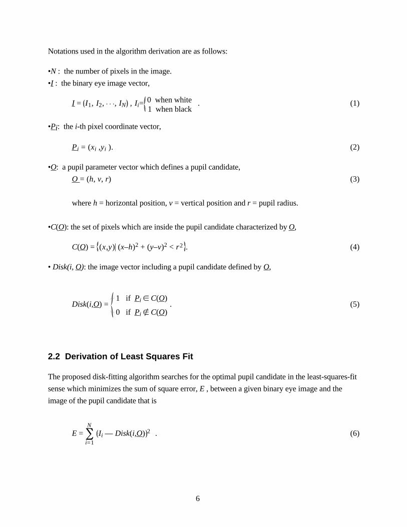
Notations used in the algorithm derivation are as follows:

•N : the number of pixels in the image.

•I : the binary eye image vector,

I = I1, I2, , IN , Ii=0 when white1 when black

. (1)

•Pi: the i-th pixel coordinate vector,

Pi = (xi ,yi ). (2)

•O: a pupil parameter vector which defines a pupil candidate,

O = (h, v, r) (3)

where h = horizontal position, v = vertical position and r = pupil radius.

•C(O): the set of pixels which are inside the pupil candidate characterized by O,

C(O) = (x,y) (x–h)2 + (y–v)2 < r2 . (4)

• Disk(i, O): the image vector including a pupil candidate defined by O,

Disk(i,O) = 1 if Pi Î C(O)

0 if Pi Ï C(O). (5)

2.2 Derivation of Least Squares Fit

The proposed disk-fitting algorithm searches for the optimal pupil candidate in the least-squares-fit

sense which minimizes the sum of square error, E , between a given binary eye image and the

image of the pupil candidate that is

E = Ii — Disk(i,O) 2åi=1

N

. (6)

7

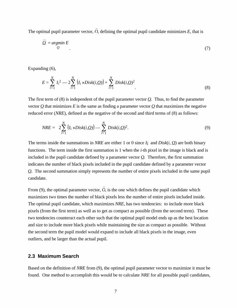
The optimal pupil parameter vector, O, defining the optimal pupil candidate minimizes E, that is

O = argminO

E. (7)

Expanding (6),

E = Ii2å

i=1

N

— 2 Ii ´Disk(i,O)åi=1

N

+ Disk(i,O)2åi=1

N

. (8)

The first term of (8) is independent of the pupil parameter vector O. Thus, to find the parameter

vector O that minimizes E is the same as finding a parameter vector O that maximizes the negative

reduced error (NRE), defined as the negative of the second and third terms of (8) as follows:

NRE = 2 Ii ´Disk(i,O)åi=1

N

— Disk(i,O)2åi=1

N

. (9)

The terms inside the summations in NRE are either 1 or 0 since Ii and Disk(i, O) are both binary

functions. The term inside the first summation is 1 when the i-th pixel in the image is black and is

included in the pupil candidate defined by a parameter vector O. Therefore, the first summation

indicates the number of black pixels included in the pupil candidate defined by a parameter vector

O. The second summation simply represents the number of entire pixels included in the same pupil

candidate.

From (9), the optimal parameter vector, O, is the one which defines the pupil candidate which

maximizes two times the number of black pixels less the number of entire pixels included inside.

The optimal pupil candidate, which maximizes NRE, has two tendencies: to include more black

pixels (from the first term) as well as to get as compact as possible (from the second term). These

two tendencies counteract each other such that the optimal pupil model ends up as the best location

and size to include more black pixels while maintaining the size as compact as possible. Without

the second term the pupil model would expand to include all black pixels in the image, even

outliers, and be larger than the actual pupil.

2.3 Maximum Search

Based on the definition of NRE from (9), the optimal pupil parameter vector to maximize it must be

found. One method to accomplish this would be to calculate NRE for all possible pupil candidates,

8

and to select the corresponding parameter vector of the candidate which generates the maximum

NRE. This method, which will be referred to as the direct search method, is computationally too

expensive to be implemented in practice since the number of all possible pupil candidates could be

enormous depending on the image size. Therefore, we need to optimize the search for the optimal

pupil parameter vector for a practical implementation of the disk-fitting algorithm.

2.3.1 Comparison Search Method

The NRE characteristic on the parameter vector space provides the basis for this optimized search.

Figure 1 illustrates three artificial pupil images and their corresponding NRE surface profiles in

two-dimensional eye position vector space. The radius of the pupil candidates used in calculating

NRE, called the search radius, is set to a specific value in each NRE surface profile. The figure

shows five NRE surface profiles with different search radii corresponding to each artificial pupil

image. The search radii are the correct radius of the pupil, the smaller radii than the correct one by

5 and 10 pixels, and the larger radii by 5 and 10 pixels. NRE surface profile with smaller search

radius is placed on the left in Figure 1 (b), (c), and (d). As shown in the figures, the general shape

of the NRE surface is an inverted cone.

For the artificial image of the pupil A in Figure 1(a) which represent noiseless eye images, the

corresponding NRE surface profiles are shown in Figure 1(b). With the search radii different from

the correct pupil radius, the NRE surface profiles have a plateau on top. The plateau gets higher

and smaller as the search radius gets closer to the true pupil radius. Then, the plateau becomes an

apex when the search radius is the same as the true pupil radius. The location of the apex in the

eye position vector space is the same as the pupil center. The pupil B in Figure 1(a) represents a

pupil with typical image noise and an artifact. The circular disk structure of the pupil is

contaminated by high frequency image noise and a Purkinje image embedded in it. The general

shape of the NRE surface profiles for the pupil B, shown in Figure 1(c), is still an inverted cone

and is very close to the one from the pupil A, even though these are slightly dented. The apex is

formed with the search radius the same as the correct pupil radius, and is located at the pupil

center. Figure 1(d) illustrates the result from a different type of image artifact consisting of three

black lines crossing the pupil in the horizontal direction and one black and one white line crossing

in the vertical direction.

9

Fig. 1(a)

Fig.1(b)

Fig.1(c)

Fig.1(d)

Figure 1. Artificial pupil images with corresponding NRE surface profiles in two-dimensional eyeposition domain. The search radius is assumed to be known: (a) three artificial pupil images, (b)NRE surface profiles for Pupil A, (c) NRE surface profiles for Pupil B, (d) NRE surface profiles forPupil C.

10

This kind of artifact seldom happens in a real situation, but is rather designed to demonstrate the

NRE characteristic. The NRE surface profiles for the pupil C closely resemble the profiles for

other pupils; the difference is the sharp dents introduced by the long and narrow image artifacts.

Again, the apex is formed with the search radius the same as the correct pupil radius, and is located

at the pupil center.

The inverted cone shape of the NRE surface profiles suggests that NRE increases gradually as the

pupil parameter vector is getting closer to the optimal one. This is also apparent when considering

(9) since a pupil candidate closer to the true pupil would include more black pixels and fewer white

pixels. The search for the optimal pupil parameter vector can thus be achieved by comparing the

NRE of the pupil candidate defined by the current parameter vector with those of its neighboring

vectors in the parameter space, and updating the current vector with the one that has the largest

NRE among neighbors. When the current parameter vector reaches the point of having a larger

NRE than its neighbors, that vector is considered to be the optimal pupil parameter vector. This

method of finding the optimal parameter vector by the comparison-update iterations will be referred

to as the comparison search method.

We can compare values of NRE from two adjacent parameter vectors in the parameter space by

inspecting only a small number of pixels. If pupil candidates defined by two parameter vectors

overlap, the common area contributes the same amount to the NRE of both candidates because two

times the number of dark pixels less the total number of pixels is fixed for this region; therefore,

only the data from the non-overlapping area needs to be compared. Figure 2 shows two cases of

overlapping pupil candidates defined by adjacent parameter vectors, where pupil candidate 1 and

pupil candidate 2 have the common area S. The case 1 of Figure 2 shows pupil candidates of the

same radius but with different center locations by d, and the case 2 shows two candidates of the

same center location with different radii by d. Comparison of NRE contributed by S1 and S2 in

the case 1, and S3 in the case 2, determines which candidate has the larger NRE since they are the

marginal areas. If the margin d between two pupil candidates is one pixel, the smallest quantized

step in image domain, then S1, S2, and S3 narrow to an area of just a few pixels. Only these

small number of pixels need to be examined to calculate NRE of marginal areas, and determine

which pupil candidate vector has the larger NRE.

11

Figure 2. Comparison of two neighboring pupil candidates illustrates a common area S. Onlycomparison of the non-overlapping regions, S1 from pupil candidate 1 and S2 from pupil candidate2, is required to compare their relative NRE.

Figure 3 illustrates the relationship between the computational savings from limiting the

comparison to these marginal regions and the size of the pupil. Based on the case 1 of Figure 2, if

the comparison of the entire area is used, every pixel in area S and S1 will be included for pupil

candidate 1, and every pixel in area S and S2 will be included for pupil candidate 2. Since the area

of S1 is equal to the area of S2, the total number of pixels included in the comparison of the entire

area would be equal to two times the sum of area S and area S1. However, by limiting the

comparison to the non-overlapping areas, the number of pixels to be included in the comparison of

two pupil candidates can be reduced to the sum of areas S1 and S2 (which is equivalent to two

times the area of S1). The difference in number of pixels required for these two approaches can be

expressed as a ratio of the size of the area S1 (corresponding to a comparison search of the non-

overlapping regions only) to the size of the area S plus area S1 (representing a search of the entire

pupil regions). As shown in Figure 3, this size ratio becomes smaller as the radius gets larger,

meaning that there are more computational savings for a larger radius. A similar relationship exists

for the case 2 of Figure 2.

12

Figure 3. Ratio of the size of areas required to compare two pupil candidates using only the non-overlapping regions (S1) versus the entire pupil areas (area S+ area S1). As shown, this size ratiovaries as a function of pupil radius.

2.3.2 Look-Up Tables for Relative Pixel Coordinates

Even though only the non-overlapping regions need to be compared, the comparison search

method still requires a large number of calculations to determine which pixels are included in the

marginal areas such as S1, S2, and S3 in Figure 2. However, if the step size d between two

parameter vectors to compare is fixed to a certain value throughout the whole search process, the

process can take advantage of a look-up table specifically designed for comparing pupil candidates

separated by the certain distance. For different geometric relationships between the current and the

neighboring pupil candidates to compare, the relative pixel coordinates in the marginal areas

relative to the center of the current pupil candidate can be predetermined and stored in different

look-up tables. Using these tables, only additions are required to determine the absolute position

of pixels in the marginal areas. Besides reducing the overall number of calculations required, the

absence of multiplication steps in the calculation is a key source of computational savings.

13

The adjacent pupil parameter vectors compared with the current one in a comparison-update

iteration may include all of the 26 surrounding grid points in 3D parameter vector space, or just the

6 surrounding points located along the three major parameter axes (horizontal position, vertical

position, and pupil radius). Both have similar converging paths for the optimal pupil candidate. In

the current system implementation, the 6-neighbor system is used with the look-up tables since it

requires fewer computations.

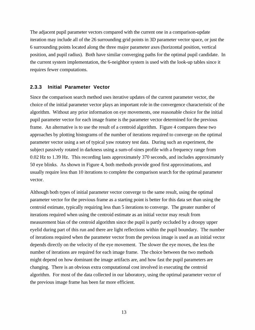
2.3.3 Initial Parameter Vector

Since the comparison search method uses iterative updates of the current parameter vector, the

choice of the initial parameter vector plays an important role in the convergence characteristic of the

algorithm. Without any prior information on eye movements, one reasonable choice for the initial

pupil parameter vector for each image frame is the parameter vector determined for the previous

frame. An alternative is to use the result of a centroid algorithm. Figure 4 compares these two

approaches by plotting histograms of the number of iterations required to converge on the optimal

parameter vector using a set of typical yaw rotatory test data. During such an experiment, the

subject passively rotated in darkness using a sum-of-sines profile with a frequency range from

0.02 Hz to 1.39 Hz. This recording lasts approximately 370 seconds, and includes approximately

50 eye blinks. As shown in Figure 4, both methods provide good first approximations, and

usually require less than 10 iterations to complete the comparison search for the optimal parameter

vector.

Although both types of initial parameter vector converge to the same result, using the optimal

parameter vector for the previous frame as a starting point is better for this data set than using the

centroid estimate, typically requiring less than 5 iterations to converge. The greater number of

iterations required when using the centroid estimate as an initial vector may result from

measurement bias of the centroid algorithm since the pupil is partly occluded by a droopy upper

eyelid during part of this run and there are light reflections within the pupil boundary. The number

of iterations required when the parameter vector from the previous image is used as an initial vector

depends directly on the velocity of the eye movement. The slower the eye moves, the less the

number of iterations are required for each image frame. The choice between the two methods

might depend on how dominant the image artifacts are, and how fast the pupil parameters are

changing. There is an obvious extra computational cost involved in executing the centroid

algorithm. For most of the data collected in our laboratory, using the optimal parameter vector of

the previous image frame has been far more efficient.

14

Figure 4. Iterations required to converge on optimal pupil model using the results from theprevious frame as initial parameters (circle marks) versus the centroid estimate of the current frameas initial parameters (cross marks).

2.4 Image Threshold

Since the disk-fitting algorithm relies on binary images derived from the gray-scale video frames,

establishing the proper threshold is important for the accuracy of the algorithm. Several techniques

have been published for choosing the optimal threshold in various senses of optimality [21]. For

the disk-fitting algorithm, a new optimality criterion is defined to minimize the least-square-fit

error. A binary eye image based on any threshold value has its own optimal parameter vector with

its associated fitting error. The optimal threshold for the disk-fitting algorithm is defined to be the

one that results in the smallest optimal fitting error. In other words, the binary image with the

15

optimal threshold produces smaller least-square-fit error than binary images with other threshold

values on the same gray-scale image.

To find the optimal threshold for a frame of pupil image, the optimal fitting error for every

threshold value must be found and compared. The fitting error is based on the error term E from

(8). This step could be an expensive operation, since up to 256 binary images from a single gray-

scale image (corresponding to 256 different gray levels) might need to be analyzed for the

corresponding optimal pupil parameters and fitting error.

However, given a fairly uniform illumination of the eye, this threshold choosing step is typically

required only once for the very first image frame of the video image frames. Also, searching a

reduced threshold set with a practical range (e.g., 100 to 250) and larger threshold step sizes (e.g.,

5) provides a pseudo-optimal threshold which has been satisfactory for most of the data collected

in our laboratory.

2.5 Subpixel Interpolation

The nature of the comparison search method causes pupil parameter values to be quantized. In the

current implementation of the disk-fitting algorithm, the three resulting parameters (horizontal and

vertical center coordinates and pupil radius) are quantized by the step size of one pixel, the smallest

screen measurement. To achieve a smooth output and a subpixel resolution, we use a quadratic

interpolation of NRE with three points on each major axis in the parameter domain. These three

points are the quantized optimal parameter value itself, the optimal parameter value plus one, and

the optimal parameter value minus one. The quadratic interpolation method has been generating a

satisfactory result, ensuring the final parameter value within a half pixel distance from the

quantized optimal parameter value.

2.6 Elliptic Appearance of Pupil

The algorithm searches for the pupil as a circular disk, and derives pupil sizes and center

coordinates based on this model. However, as the visual axis of the eye deviates from the camera

optical axis, the projection of the 3D ocular anatomy onto the two-dimensional image plane may

cause the shape of the pupil to become an ellipse. In fact, the boundary of the pupil in the image

will always be elliptical except when the eye is looking straight into the camera lens, and the

magnitude of this effect will be dependent on the angle of gaze.

16

Regardless of the radius, the circular disk concentric with an ellipse has a larger overlapped area

with the ellipse than other circular disks of the same radius. If the ellipse is a black pupil, the

concentric circular disk will have larger NRE than other disks of the same radius, since it will

include most black pixels. Thus, the optimal pupil candidate¾the circular disk with the largest

NRE¾will have the same center as the elliptic pupil.

Since an ellipse has two radial distances on its two major axes, the single radius parameter in the

pupil candidate cannot represent the size of an ellipse accurately. However, there is a certain

relationship between two radii of the ellipse and the radius of the optimal pupil candidate. The

radius of the optimal pupil candidate is not larger than the longer radius of the ellipse. If it is

larger, the pupil candidate will include more white pixels with the same number of black pixels,

thus reducing NRE. Also, the radius of the optimal pupil candidate is not smaller than the shorter

radius of the ellipse. If it is smaller, the pupil candidate loses black pixels and total pixels at the

same rate, thus reducing NRE. Therefore, the radius of the optimal pupil candidate falls between

the longer and the shorter radius of the ellipse. Figure 5 shows the optimal radius measured by the

disk-fitting algorithm when the pupil is an ellipse with the major radius of 130. The abscissa of the

graph is the minor radius of the pupil ellipse. The graph is achieved by a computer simulation

using artificial elliptic pupils with the fixed major radius of 130 and the variable minor radius. The

optimal radius by the disk-fitting algorithm is shown to be between the major and the minor radii of

the pupil ellipse. When the minor radius is the same as the major radius, the pupil becomes a

circular disk, and the optimal radius becomes the same as the pupil radius.

The disk-fitting algorithm, therefore, will find the correct center of the elliptic pupil and an

approximated radius of two elliptic pupil radii, even though the algorithm is using the perfect

circular disk model for the pupil.

17

20 40 60 80 100 120

20

40

60

80

100

120

radi

us m

easu

rem

ent

by d

isk-

fittin

g al

gorit

hm

minor radius of elliptic pupil

major radius of elliptic pupil = 130

Figure 5. Optimal radius measured by the disk-fitting algorithm when the pupil is an ellipse withthe major radius of 130. The abscissa of the graph is the minor radius of the pupil ellipse.

3.0 Performance Evaluation

3.1 Effect of Random Image Noise

This section presents the performance of the disk-fitting algorithm. The performance is expressed

in terms of the mean offset of the pupil center measurement and the standard deviation of the radius

measurement with different amounts of random image noise.

3.1.1 Method

We used four-second-long artificial eye images to calculate the mean offset of the pupil center and

the standard deviation of the radius measurement. A computer then adds a certain amount of

random image noise to the original eye images. The disk-fitting algorithm measures the pupil

centers and radii of both the original and the noise-added images. The discrepancy of the two

measurements is used as the error due to the added random image noise.

18

We generate the simulated eye images in four steps:

1. The noiseless eye image is generated.

2. Independent identically distributed (i.i.d.) Gaussian noise is added.

3. The image is blurred.

4. Another i.i.d. Gaussian noise is added.

For each set of parameters defining image fuzziness and image noise, 50 eye images are generated.

We then measure the pupil location and the radius by both the disk-fitting algorithm and the

centroid algorithm for comparison.

3.1.1.1 Pupil Model

The gray-scale artificial eye image P(x,y) is generated by

P x ,y = 50 + 190

x-xo2+ y–yo

2

r

2m+ 1

(10)

where (xo, yo) is the center coordinate and r is the radius. The power m adjusts the fuzziness on

the pupil boundary. The gray-scale eye image in (10) simulates 8-bit-deep images where the pure

black is 255 and the white is 0. With the power m of 10 to 50, (10) generates eye images similar

to real ones, as depicted in Figure 6.

Fig. 6.(a) Fig. 6.(b) Fig. 6.(c)

Figure 6. Samples of artificially generated pupil images using equation (10): (a) when m = 10, (b)when m = 30, (c) when m = 50.

3.1.1.2 Random Noises and Blurring

The first i.i.d. Gaussian random noise is then added to each pixel to simulate the random image

noise in the image-recording phase. Zero mean and different standard deviations are used to

represent different noise conditions. Then, the image is low-pass filtered by a 3-by-3 matrix B

using (11) to make the independent noise correlate in two-dimensional image space.

19

B =k

12 2

12

12 2

12

1 12

12 2

12

12 2

where k = 3 + 2 -1. (11)

Simulating the noise involved in the image grabbing phase by a framegrabber, another i.i.d.

Gaussian is then added after the low pass filtering. The mean is zero and the standard deviation is

set to be one-fourth of the first Gaussian noise, which is added before the low pass filtering.

3.1.1.3 Data Measurement

This simulation includes combinations of 5 different values of the power m and 5 different noise

standard deviations. The power m ranges from 10 through 50 by the step size of 10, and the noise

standard deviation ranges from 8 through 40 by the step size of 8. Figure 7 shows sample images

with the minimum and maximum values for these two variables. For each combination of power

m and noise level, we generate 50 images by using new sets of random noises, and analyze them

by the disk-fitting algorithm and the centroid algorithm. We use two quantities to compare the

resolutions of the two pupil-tracking algorithms: the mean offset of the pupil center measurement

and the standard deviation of the radius measurement.

The mean offset is calculated using (12),

mean offset = 1N

mi—m 2+ ni—n 2åi=1

N

(12)

where (mi, ni) is the measured pupil center coordinate from the i-th image, and (m, n) is the real

pupil center coordinate used in the simulation. N is 50 (the number of images per set). The mean

offset is the average distance between the real pupil center and the measured one. A better

measurement algorithm generates a smaller mean offset.

The other quantity used for comparison is the standard deviation of the radius measurement. Since

the gray-scale pupil model generated by (10) has a smooth edge, the radius of the pupil in the

thresholded binary image varies according to the threshold value used. Therefore, the consistency

of the radius measurement is used to evaluate the performance of the two algorithms to measure the

pupil radius.

20

Fig. 7.(a) Fig. 7.(b) Fig. 7.(c)

Fig. 7.(d) Fig. 7.(e) Fig. 7.(f)

Fig. 7.(g) Fig. 7.(h)

Figure 7. Artificial pupil images used in the simulation with their corresponding thresholded binaryimage: (a, e) m = 50, noise variance = 8; (b, f) m = 50, noise variance = 40; (c, g) m = 10, noisevariance = 8; (d, h) m = 10, noise variance = 40.

3.1.2 Simulation Results

As summarized in Figure 8, the simulation results indicate that both the disk-fitting algorithm and

the centroid algorithm generate almost identical results for images without artifacts but with

variable levels of fuzziness and random noise. As observed from Figure 8(a) and (b), the mean

offset of the center measurement is less than 0.05 pixel unless the image is very fuzzy (small

power m) with high noise variance. The standard deviation of the radius measurement from both

21

algorithms (Figure 8(c) and (d)) is also less than 0.05 pixel for most image sets. Although the

disk-fitting algorithm shows slightly better overall resolution in the pupil center coordinate

measurements, the centroid algorithm shows slightly less variance in the pupil radius

measurements. However, these differences are quite trivial. Therefore, this first simulation

suggests that, for images with only random noise and with no occlusions of the pupil area, the

measurement resolutions of the centroid and the disk-fitting algorithms are almost identical.

Fig. 8.(a) Fig. 8.(b)

Fig. 8.(c) Fig. 8.(d)

Figure 8. The performances of the disk-fitting method and centroid method are compared usingsimulated blurred images and random noise: (a) the mean of center location offset from the disk-fitting algorithm, (b) the mean of center location offset from the centroid algorithm, (c) the standarddeviation of the radius measurement by the disk-fitting algorithm, (d) the standard deviation of theradius measurement by the centroid algorithm.

22

3.2 Performance With Occlusions of the Pupil Area

Although the previous simulation accounts for fuzziness and random noise, eye images are

susceptible to more serious types of artifacts which can result in systematic measurement bias of

the pupil center coordinates or pupil radius. Such errors result from false detection of pixels

outside the true pupil area or missed detection of pixels inside the true pupil area. Two common

examples which lead to missed detection of pixels occur during occlusion of the pupil from either

light reflections or eyelids. Although different techniques have been devised to bypass these

artifacts, the performance of these techniques tends to be case-selective and subject to their own

biases when other artifacts are unaccounted for.

Certainly the robustness of a pupil-tracking algorithm to these common artifacts is critical to avoid

systematic measurement bias. The purpose of this section is therefore to analyze the performance

of the disk-fitting algorithm with two of the most frequently encountered artifacts¾the droopy

upper eyelid and a light reflection in the pupil boundary¾and to compare its performance with the

centroid algorithm using simulated eye images.

3.2.1 Effect of Droopy Eyelid on the Disk-Fitting Algorithm

It is common during routine oculomotor testing for the upper eyelid to partly cover the pupil,

especially during tests conducted in darkness to assess vestibulo-ocular reflexes, or during large

gaze shifts when fixating on targets offset vertically from the normal line of sight. A partly

covered pupil invalidates the basic assumption of the pupil model as a circular disk, and might

introduce an error in the disk-fitting algorithm. If the radius of the pupil was known a priori, this

error would be minimized since the pupil candidate with the correct radius should become

concentric with the pupil in order to include the maximum number of black pixels. However, a

number of neuronal factors can influence pupil dilation and, with the exception of pharmacological

intervention, the pupil radius is seldom constant. Therefore, with a partly occluded pupil, the disk-

fitting algorithm might underestimate the pupil radius parameter and bias the center coordinate

measurement.

Figure 9(a) illustrates this case: The eyelid is represented by the straight line on the pupil, and the

black area is the visible pupil. The pupil candidate of boundary c1 has its center on the y-axis and

extends from the bottom of the real pupil to the bottom of the eyelid. The boundary c2 is for the

real pupil. For a given search radius, the maximum NRE will be obtained when the center of the

pupil candidate is positioned along the vertical y-axis, since a pupil candidate off the axis cannot

include more black pixels than the one on the axis. Also, the bottom of the pupil candidate with the

23

maximum NRE has to meet the bottom of the pupil just like the candidate of boundary c1.

Otherwise, the candidate either misses some black pixels or includes unnecessary white pixels.

Satisfying the above-mentioned conditions, the radius of the optimal pupil candidate is no less than

the radius of boundary c1, since the candidate of boundary c1 will always contain more black

pixels than others with a smaller radius. Likewise, the radius of the optimal candidate is no larger

than the radius of boundary c2 since, otherwise, the total number of pixels would increase without

adding more black pixels. Therefore, the boundary of the optimal pupil candidate for the covered

pupil will be between the boundary c1 and c2. With these guidelines, this analysis focuses on the

behavior of NRE for pupil candidates whose boundaries are between c1 and c2. The center

positions of these candidates reside between (0,-d/2) and (0,0) using the coordinate system

introduced by Figure 9(a), where d is the distance between the top of the pupil and the edge of the

eyelid.

Figure 9(b) is a redrawn version of Figure 9(a) with the orientation change for a more convenient

arithmetic in the analysis. The smaller disk in Figure 9(b) is a pupil candidate whose boundary is

between c1 and c2 (as defined in Figure 9(a)). The true pupil is centered at the coordinate origin,

with the radius r. The left edge of the pupil candidate must meet the left edge of the true pupil at (-

r, 0) to satisfy the condition that the boundary of the optimal pupil candidate be between the

boundaries c1 and c2. The term ox represents the deviation of a candidate pupil center from the

center of the true pupil, and d is the distance from the right edge of the true pupil to the eyelid. A

non-positive d means an uncovered pupil. If d equals r, half of the pupil is covered by the eyelid.

With these structures, ox for candidates of interest whose boundaries are between the boundaries

c1 and c2 will range from 0 to d/2. When ox equals 0, the boundary of the corresponding pupil

candidate coincides with the true pupil boundary, and when ox equals d/2, it coincides with the c1

boundary. For a given amount of pupil cover, d, the measurement error is represented by the

center deviation, ox, of the optimal pupil candidate.

24

Fig. 9.(a) Fig. 9.(b)

Figure 9. Models of a pupil with partial occlusion from a droopy eyelid: (a) normal orientation,illustrating the expected range of pupil candidate sizes from the true pupil (c2) to the one with aminimal pupil radius (c1); (b) 90-degree clockwise rotation of A, showing a pupil candidatecentered at -ox with a pupil boundary between c1 and c2.

When the amount of cover, d, is less than the pupil radius, r, NRE for a pupil candidate centered at

(-ox,0) is

NRE(ox) = 2 p(r–ox)2 – area(S) – p(r–ox)2 (13)

where (r-ox) is the radius of the pupil candidate. The terms inside the large parenthesis represent

the area (or the number) of black pixels, and the area(S) is the size of the occluded area in the

candidate disk. Quantitatively, area(S) is

area(S) = 2 r – ox 2 – x + ox 2 dx

r – d

r – 2ox

= r – ox 2 acosr – d + ox

r – ox – 1

2sin 2acos

r – d + oxr – ox

(14)

for a candidate whose boundary is between c1 and c2 as shown in Figure 9.

25

Figure 10(a) shows NRE for pupil candidates between c1 and c2 as a function of the center

deviation, ox, of the pupil candidate with different amounts of pupil cover, d. The radius of the

true pupil, r, is 10. When the amount of pupil cover, d, is less than about one third of the true

pupil radius, r, the maximum of NRE occurs at ox equal to 0, meaning that the optimal pupil

candidate is concentric with the true pupil. Therefore, the disk-fitting algorithm generates no bias

in the pupil center measurement. For a larger degree of pupil occlusion, the maximum occurs at a

non-zero ox. Derivatives of these curves, shown in Figure 10 (b), show more clearly where these

maxima occur.

An analytic expression of the maximum’s location could be achieved by differentiating (14) with

respect to ox, and calculating the value of ox to make the derivative zero. Due to a calculational

difficulty in achieving this analytic expression, an approximate solution is presented using the zero

crossing points from Figure 10(b). If these zero crossing points are plotted in the (ox, d) plane,

the points approach a straight line which is

ox = 0 for 0£ d <10

310 – 0.1420 – 3.5

d – 3.5 + 0.14 for 103£ d <20

. (15)

The linear approximation (15) is based on the assumption that the radius of the true pupil is 10.

For a general radius of the true pupil, r/10 is inserted into (15), to generate

ox = 0 for 0£ d <r

3r

10 10 – 0.1420 – 3.5

10dr – 3.5 + 0.14 for r

3£ d <2r

. (16)

The generalized linear approximation (16) can be used as an approximation to predict the error

when the radius of the true pupil and the amount of pupil cover are known.

As shown in Figure 10 for a true pupil of size 10, the disk-fitting algorithm generates measurement

bias only when the pupil was occluded by more than 30% of its size. With a smaller occlusion

than 30 %, the disk-fitting algorithm measures the pupil location and size without any bias.

26

Fig. 10.(a)

Fig. 10.(b)

Figure 10. Measurement errors for pupils with a partial occlusion from a droopy eyelid can bederived by examining the value of ox at the NRE maxima. Each line represents a different amountof occlusion (defined by d): (a) the NRE graph for different amounts of occlusion; (b) derivativesof the NRE curves showing more clearly where the maxima occur (crossing the abscissa).

27

3.2.2 Effect of Light Reflection on Disk-Fitting Algorithm

The light reflection on the pupil is a major obstacle for video eye-tracking systems. The first case

to consider is when a light reflection is on the pupil boundary, and then the case will be

generalized. Figure 11 is a pupil model with a light reflection centered on the pupil edge. The

radius of the light reflection is d. With an analogous logic to the one provided in the droopy eyelid

analysis, a similar condition applies to the optimal pupil candidate.

Figure 11. Model of pupil occluded by a light reflection centered on the pupil edge. The dashedboundary depicts a pupil candidate centered at ox which is an indication of measurement error. Inthis case, d refers to the radius of the light reflection.

Using the coordinate system in Figure 11, the center coordinate of the optimal pupil candidate

should be between (0,0) and (-d/2,0), and the left end of the optimal candidate should meet the left

end of the true pupil. Based on these conditions, NRE of pupil candidates whose center (-ox,0) is

located between (0,0) and (-d/2,0) is derived for examining the center measurement bias. NRE of

a pupil candidate whose center is at (-ox,0) can be calculated using (13). The area(S) is the area

(or the number) of white pixels inside the pupil candidate, and can be determined from

area(S) = 2 d2– x – r 2 dx

r – d

x p

+ 2 r – ox 2 – x + ox 2

x p

r – 2ox

dx (17)

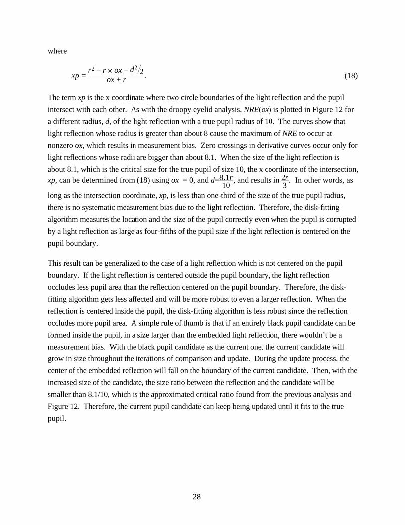
28

where

xp = r2 – r ´ ox – d2

2ox + r . (18)

The term xp is the x coordinate where two circle boundaries of the light reflection and the pupil

intersect with each other. As with the droopy eyelid analysis, NRE(ox) is plotted in Figure 12 for

a different radius, d, of the light reflection with a true pupil radius of 10. The curves show that

light reflection whose radius is greater than about 8 cause the maximum of NRE to occur at

nonzero ox, which results in measurement bias. Zero crossings in derivative curves occur only for

light reflections whose radii are bigger than about 8.1. When the size of the light reflection is

about 8.1, which is the critical size for the true pupil of size 10, the x coordinate of the intersection,

xp, can be determined from (18) using ox = 0, and d=8.1r10

, and results in 2r3

. In other words, as

long as the intersection coordinate, xp, is less than one-third of the size of the true pupil radius,

there is no systematic measurement bias due to the light reflection. Therefore, the disk-fitting

algorithm measures the location and the size of the pupil correctly even when the pupil is corrupted

by a light reflection as large as four-fifths of the pupil size if the light reflection is centered on the

pupil boundary.

This result can be generalized to the case of a light reflection which is not centered on the pupil

boundary. If the light reflection is centered outside the pupil boundary, the light reflection

occludes less pupil area than the reflection centered on the pupil boundary. Therefore, the disk-

fitting algorithm gets less affected and will be more robust to even a larger reflection. When the

reflection is centered inside the pupil, the disk-fitting algorithm is less robust since the reflection

occludes more pupil area. A simple rule of thumb is that if an entirely black pupil candidate can be

formed inside the pupil, in a size larger than the embedded light reflection, there wouldn’t be a

measurement bias. With the black pupil candidate as the current one, the current candidate will

grow in size throughout the iterations of comparison and update. During the update process, the

center of the embedded reflection will fall on the boundary of the current candidate. Then, with the

increased size of the candidate, the size ratio between the reflection and the candidate will be

smaller than 8.1/10, which is the approximated critical ratio found from the previous analysis and

Figure 12. Therefore, the current pupil candidate can keep being updated until it fits to the true

pupil.

29

Fig. 12.(a)

Fig. 12.(b)

Figure 12. Measurement errors for pupils with a partial occlusion from a light reflection can bederived by examining the value of ox at the NRE maxima. Each line represents a different amountof occlusion (defined by d): (a) the NRE graph for different amounts of occlusion; (b) derivativesof the NRE curves showing more clearly where the maxima occur (crossing the abscissa).

30

A light reflection centered on or outside the pupil boundary might shift the location of the apex in

the NRE surface profile if the reflection size is larger than the critical size. A reflection centered

inside the pupil, however, may cause a local maximum in the NRE surface profile depending on

the relative size and location with respect to those of the true pupil. Even when a local maximum

exists in the NRE surface profile, the likelihood of a false convergence on the local maximum is

dependent on the choice of the initial current pupil candidate. Provided an initial search radius

close to the true pupil radius, the comparison search will converge on the true pupil parameters

even with a larger light reflection.

3.2.3 Comparison of Centroid and Disk-Fitting Algorithms With

Simulated Artifacts

To compare the robustness of the disk-fitting algorithm relative to the centroid algorithm, we used

both algorithms to analyze simulated eye images which are generated using a combination of

artifacts. Simulated eye image is created using (10) with a power m for fuzziness control set to 20

and noise standard deviation set to 20. We generated 120 simulated eye images with a pupil at

different locations and three kinds of artifacts at fixed locations. As illustrated in Figure 13, these

artifacts include an upper eyelid partly occluding the upper part of the pupil, three light reflections

of various sizes, and a shadow along the bottom part of the pupil. The different positions of the

artificial pupils simulate a sinusoidal eye movement in the horizontal plane at 0.5 Hz (based on

120 samples over 2 sec) at an amplitude of 15 pixels. The vertical position and the radius are fixed

throughout the simulation.

31

Figure 13. Artificial pupil images used in the simulation with their corresponding thresholdedbinary image: (a)(b) pupil positioned far left, (c)(d) pupil at center, (e)(f) pupil positioned far right.The image size was 120 by 120 pixels. The vertical center coordinate and the radius are set to be 60and 40, respectively, with the origin at the upper left corner. The upper eyelid covers all pixelswhose vertical coordinate is less than 24 (i.e. d = 4). The horizontal center, vertical center, andradius for the reflections are (88, 35, 9), (60, 45, 7) and (20, 65, 5). The maximum width of theshadow is 5 pixels.

Figure 14 depicts the horizontal and vertical measurement errors from both algorithms. As shown

in these graphs, the error from the disk-fitting algorithm is not only substantially smaller than the

centroid algorithm, but was also more homogeneous with no apparent pattern. The centroid

algorithm, on the other hand, is highly sensitive to the artifacts, and the measurement error varies

32

as a function of the pupil position relative to the artifact positions. This error variability could lead

to a wrong scientific interpretation of eye movement data since the magnitude of distortion depends

on the amount of pupil occlusion which can systematically vary with eye position.

horizonta l error in pixel

t ime

Fig. 14.(a)

verti cal error in pixel

t ime

Fig. 14.(b)

Figure 14. Measurement errors from the disk-fitting algorithm and centroid algorithm during asimulation of horizontal sinusoidal eye movements, (a) the errors of horizontal center measurement;(b) the errors of vertical center measurement.

33

The performance analysis using blurred images with random noise (in section 3.1) suggests that

both algorithms have a resolution of approximately 0.05 pixels. The results from this simulation

differ in that the error from the centroid algorithm can be in the order of several pixels when

artifacts either obscure part of the pupil or create shadows in the image. Although the disk-fitting

algorithm also generates slightly larger errors with these more obtrusive artifacts, the superior

performance of this algorithm even with these artifacts is quite compelling. Simulations with these

types of artifacts are more reasonable approximations to what can be expected in actual test

environments.

4.0 Implementation and Examples

We implemented the disk-fitting algorithm using a personal computer system. As illustrated in

Figure 15, the system comprises a personal computer as a host-processing unit, three computer

interface boards (framegrabber board, fast memory board, and digital signal processing board) and

a computer controlled videocassette recorder (VCR). The current system uses off-line image

analysis of videotapes to provide a more flexible programming environment for algorithm

enhancement. Routines to automatically preset threshold parameters and adjust template settings

have enabled the implementation of a batch processing capability. A video time-code inserter

allows the use of a common time-code for synchronization with other signals, such as stimulus

waveforms, which are archived in separate files.

Video Tape

Serial Port

VCR

Framegrabber

Fast Memory

DSP

Serial Port Hard Drive

CPU

HOST COMPUTER

LookUpTables

EyeData

VDACsoftware

Display ControlMonitor

........................................

....

..............................

Figure 15. Block diagram of the VDAC system illustrating the flow of images through the frame-grabber (solid lines), and the flow of software data (dashed lines) and control signals (dotted lines).

34

While analyzing videotapes, the host computer controls the VCR to feed a certain number of

images to the memory board through the framegrabber. The system has currently been

implemented with NTSC format, and it analyzes even and odd fields of the image separately to

support a 60 Hz sampling rate. It then analyzes the images stored in the memory using the disk-

fitting algorithm to track the pupil. Following gray-scale capturing of a video field, the system

creates a binary image by thresholding on the pupil gray-scale level. The disk-fitting algorithm is

used with this binary image to derive the horizontal and vertical coordinates of pupil center and

pupil radius. Look-up tables (described later) are retrieved from computer memory to optimize the

search for optimal pupil parameters. Large step changes in the pupil radius parameter are used to

flag periods during eye blinks as an aid for further data processing. A flexible user interface

allows the user to set up run parameters for batch processing, and to customize the display to

monitor the tracking performance on line.

We can easily expand the system to add other processing steps, such as geometrical correction to

account for elliptical distortions and torsion measurements from the iris pattern. For example, we

currently retain the gray-scale image to derive counterroll measurements. Upon locating the pupil

center, cross-correlations of multiple one-dimensional templates on a partial annulus overlying the

iris are used to calculate ocular torsion [13].

A recent speed test on a Power Macintosh 8100/110 platform showed that it takes less than 1/60th

of a second to track the size and location of the pupil only and slightly more than that to include

torsion calculations. The test proved that the disk-fitting algorithm with a torsion calculation could

be implemented into a real-time system with proper code optimization and modification of image-

handling interfaces.

The system with the disk-fitting algorithm has been used for analyzing video eye images of more

than 30 hours from various experiments of the NASA Neurosciences Laboratory. The quality of

the video eye image varies considerably depending on the type of camera, the subject, and the

operator of each experiment. Figures 16(a) and (b) show two types of video eye images collected

during the experiments. Figure 16(a) is a snapshot of one of the best quality images, and Figure

16(b) is of the worst quality images. Obviously, the counterroll measurement is not possible with

the video eye images like Figure 16(b) since the image is too smeared and no iris pattern is visible.

35

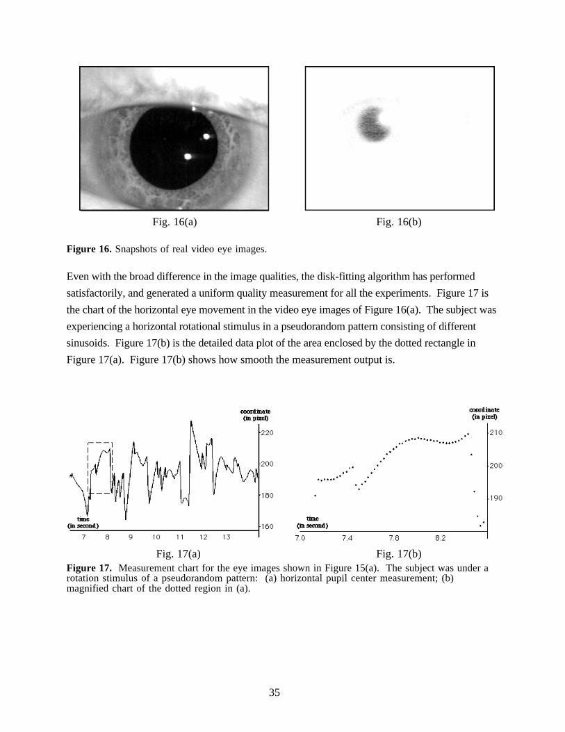
Fig. 16(a) Fig. 16(b)

Figure 16. Snapshots of real video eye images.

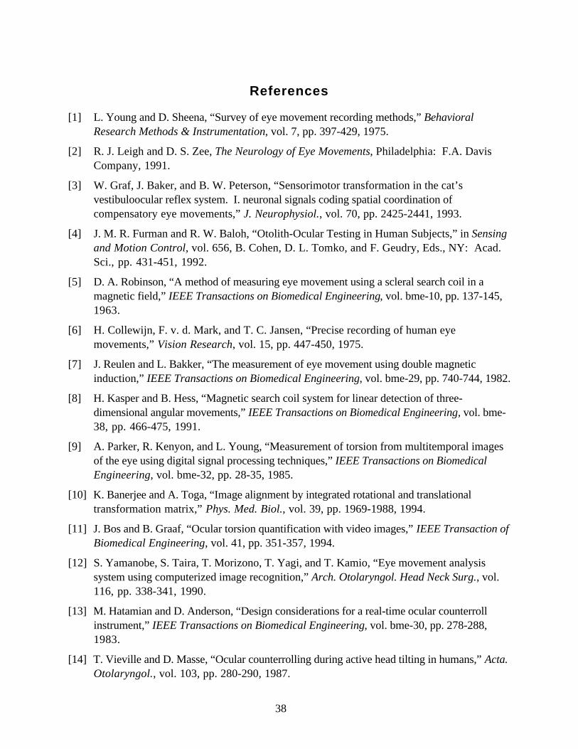
Even with the broad difference in the image qualities, the disk-fitting algorithm has performed

satisfactorily, and generated a uniform quality measurement for all the experiments. Figure 17 is

the chart of the horizontal eye movement in the video eye images of Figure 16(a). The subject was

experiencing a horizontal rotational stimulus in a pseudorandom pattern consisting of different

sinusoids. Figure 17(b) is the detailed data plot of the area enclosed by the dotted rectangle in

Figure 17(a). Figure 17(b) shows how smooth the measurement output is.

Fig. 17(a) Fig. 17(b)Figure 17. Measurement chart for the eye images shown in Figure 15(a). The subject was under arotation stimulus of a pseudorandom pattern: (a) horizontal pupil center measurement; (b)magnified chart of the dotted region in (a).

36

Figure 18 is the chart of the vertical eye movement in the video eye image of Figure 16(b). Figure

18(b) is the detailed version of the dotted area in Figure 18(a). In that experiment, the subject was

looking at the vertically moving targets, and regaining a fixation point time to time. Even though a

large reflection occludes the pupil and the pupil edges are smeared as in Figure 16(b), the disk-

fitting algorithm generated smooth output without a systematic bias.

Fig. 18(a) Fig. 18(b)

Figure 18. Measurement chart for the eye images shown in Figure 15(b). The subject was staring atvertically moving visual targets: (a) vertical pupil center measurement; (b) magnified chart of thedotted region in (a).

5.0 Conclusions

As shown in the performance analysis section, the disk-fitting algorithm is quite robust to common

image artifacts such as the droopy eyelid and light reflections while maintaining the same

measurement resolution with the centroid algorithm, which is about 0.05 pixel. Even when about

30% of the pupil area is occluded, the disk-fitting algorithm can measure the location and size of

the pupil with reasonable accuracy. The disk-fitting algorithm has successfully performed in our

laboratory with a variety of diagnostic test data. We have used it for measurements of pathologic

nystagmus (spontaneous, gaze-evoked, positional), measurements of visual-oculomotor control

(smooth pursuit, optokinetic nystagmus), and with rotational tests of vestibulo-ocular reflex

function. We have further demonstrated the robustness of the algorithm in practice in its ability to

track relatively poor eye video data which other commercial systems have failed to track.

37

Following the precise measurement of the pupil center, iris tracking techniques can then be

implemented to derive torsion position of the eye. In the system implementation in our lab, a

torsion calculation algorithm based on cross calculation of iris mark is incorporated into the disk-

fitting algorithm. The disk-fitting algorithm therefore provides a platform for a non-invasive,

multidimensional eye movement capability which can be used to assess a variety of complex eye

movements. This algorithm should prove especially useful in clinical applications for the diagnosis

of pathology associated with complex neuronal networks involved in the vestibular and oculomotor

reflex pathways, and will enable further scientific investigations and technology development

requiring the precise recording of eye movements in 3D space.

38

References

[1] L. Young and D. Sheena, “Survey of eye movement recording methods,” BehavioralResearch Methods & Instrumentation, vol. 7, pp. 397-429, 1975.

[2] R. J. Leigh and D. S. Zee, The Neurology of Eye Movements, Philadelphia: F.A. DavisCompany, 1991.

[3] W. Graf, J. Baker, and B. W. Peterson, “Sensorimotor transformation in the cat’svestibuloocular reflex system. I. neuronal signals coding spatial coordination ofcompensatory eye movements,” J. Neurophysiol., vol. 70, pp. 2425-2441, 1993.

[4] J. M. R. Furman and R. W. Baloh, “Otolith-Ocular Testing in Human Subjects,” in Sensingand Motion Control, vol. 656, B. Cohen, D. L. Tomko, and F. Geudry, Eds., NY: Acad.Sci., pp. 431-451, 1992.

[5] D. A. Robinson, “A method of measuring eye movement using a scleral search coil in amagnetic field,” IEEE Transactions on Biomedical Engineering, vol. bme-10, pp. 137-145,1963.

[6] H. Collewijn, F. v. d. Mark, and T. C. Jansen, “Precise recording of human eyemovements,” Vision Research, vol. 15, pp. 447-450, 1975.

[7] J. Reulen and L. Bakker, “The measurement of eye movement using double magneticinduction,” IEEE Transactions on Biomedical Engineering, vol. bme-29, pp. 740-744, 1982.

[8] H. Kasper and B. Hess, “Magnetic search coil system for linear detection of three-dimensional angular movements,” IEEE Transactions on Biomedical Engineering, vol. bme-38, pp. 466-475, 1991.

[9] A. Parker, R. Kenyon, and L. Young, “Measurement of torsion from multitemporal imagesof the eye using digital signal processing techniques,” IEEE Transactions on BiomedicalEngineering, vol. bme-32, pp. 28-35, 1985.

[10] K. Banerjee and A. Toga, “Image alignment by integrated rotational and translationaltransformation matrix,” Phys. Med. Biol., vol. 39, pp. 1969-1988, 1994.

[11] J. Bos and B. Graaf, “Ocular torsion quantification with video images,” IEEE Transaction ofBiomedical Engineering, vol. 41, pp. 351-357, 1994.

[12] S. Yamanobe, S. Taira, T. Morizono, T. Yagi, and T. Kamio, “Eye movement analysissystem using computerized image recognition,” Arch. Otolaryngol. Head Neck Surg., vol.116, pp. 338-341, 1990.

[13] M. Hatamian and D. Anderson, “Design considerations for a real-time ocular counterrollinstrument,” IEEE Transactions on Biomedical Engineering, vol. bme-30, pp. 278-288,1983.

[14] T. Vieville and D. Masse, “Ocular counterrolling during active head tilting in humans,” Acta.Otolaryngol., vol. 103, pp. 280-290, 1987.

39

[15] S. Moore, I. Curthoys, and S. McCoy, “VTM-an image processing system for measuringocular torsion,” Computer Methods and Programs in Biomedicine, vol. 35, pp. 219-230,1991.

[16] H. Scherer, W. Teiwes, and A. Clarke, “Measuring three dimensions of eye movement indynamic situations by means of videooculography,” Acta.Otolaryngol., vol. 111, pp. 182-187, 1991.

[17] K. Sung and D. Anderson, “Analysis of two video eye tracking algorithms,” presented atIEEE EMBS conference, Orlando, FL, 1991.

[18] G. Myers, K. Sherman, and L. Stark, “Eye monitor,” in IEEE Computer Magazine, vol.March, 1991, pp. 14-21.

[19] R. Hall, “Image processing algorithms for eye movement monitoring,” Computers andBiomedical Research, vol. 16, pp. 563-579, 1983.

[20] D. Ott, F. Gehle, and R. Eckmiller, “Video-oculographic measurement of 3- dimensional eyerotations,” J. Neuroscience Methods, vol. 35, pp. 229-234, 1990.

[21] Sahoo, T., Soltani, S., Wong, A., Chen, Y., "A Survey of Thresholding Techniques," inComputer Vision, Graphics, and Image Processing, vol. 41, pp. 233-260, 1988.