Embed Size (px)
Citation preview
A MODEL AND FINITE ELEMENT IMPLEMENTATION
FOR THE THERMO-MECHANICAL ANALYSIS OF
POLYMER COMPOSITES EXPOSED TO FIRE
Z. Zhang and S.W. Case
Materials Response Group, Department of Engineering Science & Mechanics
Virginia Polytechnic Institute and State University
225 Norris Hall, Blacksburg, VA 24061 USA
J. Lua
Global Engineering and Materials, Inc.
33 Wood Avenue South, Suite 600, Iselin, NJ 08830 USA
SUMMARY
A three-dimensional model is developed to predict the thermo-mechanical response of
polymer composites with a wide temperature range. Effects of viscoelasticity,
decomposition, and gas pressure in the solid are included. The model is incorporated
into the commercial software ABAQUS.
Keywords: Polymer composites; Thermo-mechanical response; Model; Finite element;
Fire; Viscoelasticity; Decomposition
OVERVIEW
Increased utilization of composite materials in situations where fire is a concern requires
the ability to predict the structural-mechanical response of composites subjected to
different fire scenarios. Thermal models based on different assumption were proposed
by Henderson [1-4]. Looyeh [5] included the gas pressure effect in the deformation
equation and Sullivan [6] extended the thermal model with decomposition into the
three-dimensional world. The mechanical properties of composites during and after
intense fire exposure were investigated in [7-9], while studies [10-12] focused on
compression creep rupture behavior of composites subjected to relatively low levels of
heat flux. The incremental form of the viscoelastic constitutive equation for numerical
implementation was developed in [13].
In this work, a three-dimensional model to predict the thermo-mechanical behaviour of
polymer composites over temperature ranges from below the glass transition
temperature to temperatures above the decomposition temperature is presented. The
decomposition reaction and the storage of decomposition gases in the solid are
considered in the heat transfer equation and the gas diffusion equation. The effects of
viscoelasticity and decomposition are included in the material constitutive equation. The

model is incorporated into the commercial software ABAQUS by the UMAT and
UMATHT subroutines. The code is verified and validated by comparing its results with
other numerical results and experimentally measured data.
MODEL DEVELOPMENT AND FINITE ELEMENT IMPLEMENTATION
There are four governing equations in the model: the heat transfer equation, the
decomposition equation, the gas diffusion equation, and the material constitutive
equation.
The thermal part of the model is based on [2, 5, 6] and is described by Eq. (1-3) where
m is the remaining solid mass, gm is the mass of gas, V is the control volume, pC is
the specific heat of solid, pgC is the specific heat of gas, iγ and (1 )i ig isk k kφ φ= + −
(i=1,2,3) are the permeability and thermal conductivity of composites in three
coordinate directions, igk , isk , and φ are the thermal conductivity of gases, the thermal
conductivity of solids, and the porosity of composites, µ is the viscosity of
decomposition gas, r
T
pT
h Q C dT= + ∫ is enthalpy of solid, Q is heat of decomposition,
r
T
g pgT
h C dT= ∫ is enthalpy of gas, A is pre-exponential factor, E is activation energy,
R is gas constant, n is order of reaction, 0m is initial mass, and fm is final mass. The
thermal properties of the solid material, the porosity, and the permeability are assumed
to be functions of temperature and decomposition factor. The decomposition factor F
is defined by ( ) ( )0/f fF m m m m= − − .
For the stress analysis, the material is assumed to be composed of virgin material and
char material. The material constitutive equation is given by Eq. (4). The viscoelasticity
of virgin material is described by the first term on the right hand side of Eq. (4) where
( )'m
jε ξ is the mechanical strain given by Eq. (5) in which t
jε is total strain, th
jε is
thermal strain, jα is the coefficient of thermal expansion, T is the temperature, and rT
is the reference temperature. Further, each of the stiffness quantities of virgin material is
expanded in a Prony series Eq. (6) where M is the number of Prony series terms and ξ is the temperature-reduced time defined by Eq. (7) in which Ta is temperature shift
factor. The second term on the right hand side of Eq. (4) represents the contribution of
char material. Since the stiffness of char material is assumed to be very small, this term
is neglected.
In solving these governing equations Eq. (1-4), we must determine strains, temperature,
remaining solid mass, and gas pressure. In order to implement the model into ABAQUS,
two overlaid layers of elements are employed. These elements have their displacement
degrees of freedom fixed to each other at the nodes. The solution procedure employs

one UMAT subroutine and one UMATHT subroutine applied to the first layer to define
the constitutive, decomposition, and heat transfer equations. Another UMATHT
subroutine is applied to the second layer to solve the gas diffusion equation.
NUMERICAL VERIFICATION AND EXPERIMENTAL VALIDATION
Temperature Validation
To verify the analysis implementation, we first assume there is no accumulation of
decomposition gases in the solid material. In this case, the thermal part of the model is
reduced to the model presented in [1]. In order to compare with results from the one-
dimensional model, we assume all gases flow in only one direction in three-dimensional
model. The reduced heat transfer equation is given by Eq. (8). The validation problem
consists of a sample with a heat flux applied to one side surface. Results are validated
by comparing temperature profiles obtained with those measured experimentally, as
well as those developed analytically in [14]. Fig. 1 shows the good match of
temperature history curves at the exposed surface, the middle face, and the unexposed
surface.
Gas Pressure Validation
Another validation analysis for the one-sided heating test presented in [4] was
conducted by employing two overlaid layers of elements. One UMAT and one
UMATHT were applied on the first layer to implement the constitutive equation, the
decomposition equation, and the heat transfer equation, while another UMATHT was
applied on the second layer to implement the gas diffusion equation. The geometry
model of this problem is shown in Fig. 2. There are 60 elements along 3cm thickness.
Thermal conductivity and permeability in three directions are set to be the same value.
The temperature and pressure boundary conditions on the exposed and unexposed
surface, as well as the material properties, are the same as shown in [4]. The boundary
conditions on the other surfaces are the thermal insulation and the pressure insulation
defined as zero pressure gradients with respect to the corresponding coordinates. Both
the porosity and permeability are calculated by the rule of mixture as a function of
decomposition factor. Fig. 3 shows the comparison of pressure history curves at two
different positions along the thickness. It is found that the peak of the predicted pressure
at the position close to the exposed surface is lower than the numerical results and
measured data presented in the reference. For the position away from the exposed
surface, the predicted pressure peak is closer to the measured data than the numerical
results from the reference. The peak differences between Henderson calculated results
and the predicted pressure of this model are caused by the different permeability models
and the assumption of thermochemical expansion.
Parametric Studies of Porosity and Permeability
The effects of porosity and permeability are investigated by comparing temperature
history curves at different positions and pressure distribution curves along the thickness
at different moments. There are five different setting cases for porosity and permeability

as listed in Table 1. The data in the first case are the same as data in [2]. The final
permeability increases by one order of magnitude in the second case. The third case has
larger final porosity than the second case. The porosity is set to be zero and the final
permeability is very large in the fourth case. The model used in the fifth case assumes
there is no accumulation of decomposition gases in the solid material.
Fig. 4 shows the temperature history curves obtained from the first three cases.
Permeability affects temperature little even the permeability difference reaches one
order of magnitude, while porosity has a stronger influence on temperature results.
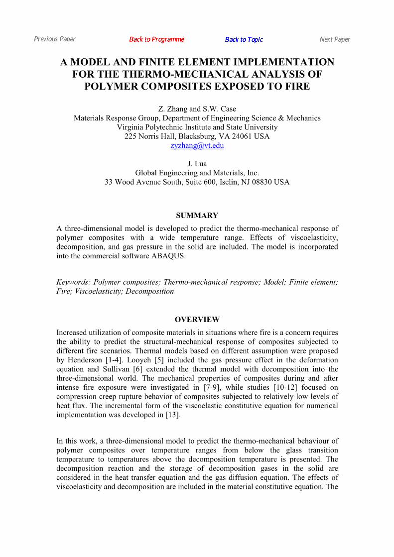
From the pressure curves in Fig. 5, we can see that pressure decreases with increasing
permeability for the same porosity, since larger permeability leads to less accumulation
of gases and the pressure is hard to build up. Pressure also decreases with increasing
porosity for the same permeability. The reason is that larger porosity makes the gas
volume increase and pressure drop. If we assume zero porosity and very large
permeability like the setting in the fourth case, there is little accumulation of the gases
in solid and the gage pressure inside the solid would keep zero. So that there is little
pressure influence on temperature and the temperature profiles are very close to the
temperature prediction from the model assuming no accumulation of decomposition
gases as shown in Fig. 6.
Validation of One-sided Heat Flux Experiments
The viscoelastic constitutive equation in the model is implemented into ABAQUS by
UMAT subroutine and has been verified before the validation problem by comparing
the shear strain obtained from this model to the theoretical results for the pure shear
creep test.
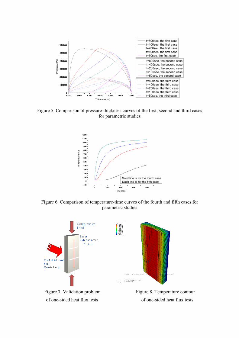
The compression creep rupture tests subject to the one-sided heat flux as shown in Fig.
7 were simulated. A heater is employed to apply a heat flux to one side of the sample
after the compressive load is ramped to the target constant value. Material properties
were measured in [15]. The test samples were the warp aligned coupons with 10 layers
in [10] and the laminate coupons [0/+45/90/45/0]s in [12]. In these tests, the temperature
is not high enough to cause significant decomposition so that viscoelasticity dominates
the mechanical behavior and the decomposition can be neglected. In this case, the
material constitutive equation can be reduced to Eq. (9).
The time and temperature dependent compression strength model of [10] is used to
calculate the compression strength in Eq. (10). Considering the material is the woven
glass fiber composite, the failure condition at each integration point is defined as Eq.
(11) where cX is the compression strength. Once the failure condition is satisfied, the
stiffness at the point is decreased to a very small value and there is no stress at the point.
Fig. 8 shows the temperature contour and Fig. 9 compares the predicted temperature at
the hot and cold surface with experimentally measured data for 5kW/m2 heat flux. The

predicted compression strain on the cold surface is compared with the measured data for
the different stress levels and the same heat flux as shown in Fig. 10. Since the
progressive failure analysis is included in the code, the compression strain increases
dramatically as the measured data at the end of the tests. The measured and predicted
times-to-failure are organized in Table 2 and plotted in Fig. 11. It is found that there is
very good agreement between the measured and predicted failure times.
CONCLUSIONS
A three-dimensional model for the prediction of thermo-mechanical response of
polymer composites was incorporated into ABAQUS by the UMAT and UMATHT
subroutines. The thermal part of the model was validated by comparing the predicted
temperature and pressure with other numerical results and experimentally measured data.
Parametric studies of porosity and permeability were conducted. It is found that the
permeability affects temperature little though the porosity has a stronger influence on
temperature. The gas pressure decreases with increasing permeability and porosity. The
one-sided heat flux tests with temperature lower than the decomposition temperature
were simulated. The mechanical part of the model was validated by comparing the
predicted temperature at the hot and cold surface, the predicted compression strain on
the cold surface, and the predicted time-to-failure with the measured data. Future efforts
will focus on the validation of the model for the one-sided heat flux tests with the
intense heating and the occurrence of significant decomposition.
0 500 1000 1500 2000 2500 3000
0
100
200
300
400
500
0 500 1000 1500 2000 2500 3000
0
100
200
300
400
500
0 500 1000 1500 2000 2500 3000
0
100
200
300
400
500
Temperature (
0C)
Time (sec)
Calculated temperature at cold face from the paper (x=9.0mm)
Calculated temperature at middle face from the paper (x=4.5mm)
Calculated temperature at hot face from the paper (x=0.0mm)
Measured temperature at cold face from the paper (x=9.0mm)
Measured temperature at middle face from the paper (x=4.5mm)
Measured temperature at hot face from the paper (x=0.0mm)
q=25kw/m2
Calculated temperature at cold face from the model (x=9.0mm)
Calculated temperature at middle face from the model (x=4.5mm)
Calculated temperature at hot face from the model (x=0.0mm)
Figure 1. Comparison of temperature history curves at the exposed surface, the middle
face, and the unexposed surface in the temperature validation study

Figure 2. Geometric model of the pressure validation problem
-100 0 100 200 300 400 500 600 700 800 900
0
1
2
3
4
5
6
7
8
9
10
Henderson experimental data
Henderson predicted pressure
Predicted pressure from this model
Gas pressure (P/Patm)
Time (sec)
-100 0 100 200 300 400 500 600 700 800 900
0
1
2
3
4
5
6
7
8
9
10
11
12
13
14
15
16
Henderson experimental data
Henderson predicted pressure
Predicted pressure from this model
Gas pressure (P/Patm)
Time (sec)
X=0.6cm X=2.25cm
Position close to the exposed surface Position away from the exposed surface
Figure 3. Comparison of pressure history curves at two different positions
0 200 400 600 800
0
200
400
600
800
1000
1200
0 200 400 600 800
0
100
200
300
400
500
600
700
800
900
1000
1100
1200
0 200 400 600 800
0
100
200
300
400
500
600
700
800
900
1000
1100
1200
x=0.1cm, the first case
x=2.0cm, the first case
x=2.5cm, the first case
x=2.9cm, the first case
Temperature (0C)
Time (sec)
x=0.1cm, the second case
x=2.0cm, the second case
x=2.5cm, the second case
x=2.9cm, the second case
x=0.1cm, the third case
x=2.0cm, the third case
x=2.5cm, the third case
x=2.9cm, the third case
Figure 4. Comparison of temperature-time curves of the first, second and third cases for
parametric studies
0.000 0.005 0.010 0.015 0.020 0.025 0.030
0
1000000
2000000
3000000
4000000
5000000
6000000
0.000 0.005 0.010 0.015 0.020 0.025 0.030
0
1000000
2000000
3000000
4000000
5000000
6000000
0.000 0.005 0.010 0.015 0.020 0.025 0.030
0
1000000
2000000
3000000
4000000
5000000
6000000
Pressure (Pa)
Thickness (m)
t=800sec, the first case
t=400sec, the first case
t=200sec, the first case
t=100sec, the first case
t=50sec, the first case
t=800sec, the second case
t=400sec, the second case
t=200sec, the second case
t=100sec, the second case
t=50sec, the second case
t=800sec, the third case
t=400sec, the third case
t=200sec, the third case
t=100sec, the third case
t=50sec, the third case
Figure 5. Comparison of pressure-thickness curves of the first, second and third cases
for parametric studies
0 200 400 600 800
-100
0
100
200
300
400
500
600
700
800
900
1000
1100
1200
0 200 400 600 800
-100
0
100
200
300
400
500
600
700
800
900
1000
1100
1200
Temperature (C)
Time (sec)
Solid line is for the fourth case
Dash line is for the fifth case
Figure 6. Comparison of temperature-time curves of the fourth and fifth cases for
parametric studies
Figure 7. Validation problem Figure 8. Temperature contour
of one-sided heat flux tests of one-sided heat flux tests

0 500 1000 1500
20
40
60
80
100
120
140
0 500 1000 1500
20
40
60
80
100
120
140
0 500 1000 1500
20
40
60
80
100
120
140
0 500 1000 1500
20
40
60
80
100
120
140
0 500 1000 1500
20
40
60
80
100
120
140
0 500 1000 1500
20
40
60
80
100
120
140
Predicted temperature at the cold surface
Predicted temperature at the hot surface
Temperature (C)
Time (sec)
Measured temperature at the hot surface
Measured temperature at the cold surface
Figure 9. Comparison of temperature at the hot and cold surface for 5kW/m2 heat flux
0 500 1000 1500 2000 2500 3000
-0.020
-0.015
-0.010
-0.005
0.000
0 500 1000 1500 2000 2500 3000
-0.020
-0.015
-0.010
-0.005
0.000
Predicted at 53.2MPa
Predicted at 56.0MPa
Predicted at 63.3MPa
Predicted at 81.8MPa
Predicted at 109.2MPa
Compression strain
Time (sec)
Measured at 53.2MPa
Measured at 56.0MPa
Measured at 63.3MPa
Measured at 81.8MPa
Measured at 109.2MPa
Figure 10. Comparison of compression strain on the cold surface for 5kW/m
2 heat flux
Figure 11. Comparison of the measured and predicted failure times

Table 1. Different cases of porosity and permeability for parametric studies
Case
number
Initial
porosity
Final
porosity
Initial permeability
(m2)
Final permeability
(m2)
1 0.113 0.274
2 0.113 0.274
3 0.113 0.6
4 0 0
5 Model in [1] assuming no accumulation of decomposition gases in the
solid material
Table 2. Comparison of the measured and predicted failure times
Warp-alinged samples
Heat Flux
(kW/m2)
5 10
Compression
Stress (MPa)
53.2 56.0 63.6 81.8 109.2 8.6 15.2 30.0 43.5 120.9
Measured Failure
Time (sec)
2957 1430 821 490 360 563 259 190 168 120
Predicted Failure
Time (sec)
1300 1220 1200 670 430 520 440 345 310 160
Heat Flux (kW/m2) 15
Compression Stress (MPa) 7.9 29.7 57.8 57.8 88.1
Measured Failure Time (sec) 568 120 95 132 87
Predicted Failure Time (sec) 230 185 148 160 124
Quasi-isotropic laminates
Test 1 2 3 4 5 6 7 8 9 10
Measured
Failure
13206 10823 3957 295 669 686 923 900 3300 5012
182.6 10−× 161.14 10−×
182.6 10−×151.14 10−×
182.6 10−× 151.14 10−×
182.6 10−× 01.14 10×

Time (sec)
Predicted
Failure
Time (sec)
5100 5400 2600 520 440 640 750 1080 1300 2800
[ ]
( ) 01
1
321
321
=∂∂
−+∇•
∂∂
+∂∂
+∂∂
−
∂∂
+∂∂
+∂∂
•∇−∂∂
+
t
mhh
VT
z
P
y
P
x
PC
RT
PM
z
Tk
y
Tk
x
Tk
t
TCmmC
V
gpg
pggp
kji
kji
µγ
µγ
µγ
(1)
( / )
0 0
1n
f E RTm mm
A em t m
−− ∂= −
∂ (2)
0
1321 =
∂
∂+
∂∂
+
∂∂
+∂∂
+∂∂
•∇−t
m
t
m
Vz
P
y
P
x
P g
g kjiµγ
µγ
µγ
ρ (3)
( )
0
( )( ) 1 ( ) ( )
m
jv c m
i ij ij jF C d FCξ ε ξ
σ ξ ξ ξ ξ ε ξξ
′∂′ ′= − − +
′∂∫ (4)
( )m t th t
j j j j j rT Tε ε ε ε α= − = − − (5)
/
1
( ) ijm
Mv
ij ij ijm
m
C C C eξ τξ −
∞=
= +∑ (6)
0
1( )
t
T
t da
ξ ξ τ= = ∫ (7)
( ) 011
321 =∂∂
−+∂∂
+
∂∂
+∂∂
+∂∂
•∇−∂∂
t
mhh
Vx
TCm
z
Tk
y
Tk
x
Tk
t
TmC
Vgpggp
ɺkji (8)
0
( )( ) ( )
m
jv
i ijC dξ ε ξ
σ ξ ξ ξ ξξ
′∂′ ′= −
′∂∫ (9)
111
12
/3( , ) ( , ) 1
7 1
n
nnk MC Yc k kt T G t T n
n
φ γσ
−− = + −
(10)
1 2max( , )cX σ σ< (11)

ACKNOWLEDGEMENTS
The authors would like to acknowledge the support of the Office of Naval Research
under the Naval International Cooperative Opportunities in Science and Technology
Program and Global Engineering and Materials, Inc. The opinions presented here are
those of the authors.
References
1. Henderson, J.B. Wiebelt, J.A. and Tant, M.R.. “A Model for the Thermal
Response of Polymer Composite Materials with Experimental Verification.”
Journal of Composite Materials 19(6) (1985): 579-595.
2. Henderson, J.B. and Wiebelt, J.A.. “A Mathematical Model to Predict the
Thermal Response of Decomposing, Expanding Polymer Composites.” Journal
of Composite Materials 21(4) (1987): 373-393.
3. Henderson, J.B. and Wiebelt, J.A.. “A numerical study of the thermally-induced
response of decomposing, expanding polymer composites” Waerme- und
Stoffuebertragung 22(5) (1988): 275-284.
4. Florio, J., Jr. Henderson, J.B. Test F.L. and Hariharan, R.. “A study of the
effects of the assumption of local-thermal equilibrium on the overall thermally-
induced response of a decomposing, glass-filled polymer composite.”
International Journal of Heat and Mass Transfer 34(1) 1991: 135-147.
5. Looyeh, M.R.E. Salamon, A. Jihan, S. and McConnachie, J.. “Modelling of
Reinforced Polymer Composites Subject to Thermo-mechanical Loading.”
International Journal for Numerical Methods in Engineering 63 (2005): 898-
925.
6. Sullivan, R.M. and Salamon, N.J.. “A Finite Element Method for the
Thermochemical Decomposition of Polymer Materials – I. Theory.”
International Journal of Engineering Science 30(4) (1992) 431-441.
7. Mouritz, A.P. and Mathys, Z.. “Post-fire Mechanical Properties of Glass-
reinforced Polyester Composites.” Composites Science and Technology 61(4)
(2001): 475-490.
8. Mouritz, A.P. and Mathys, Z.. “Mechanical Properties of Fire-damaged Glass-
reinforced Phenolic Composites.” Fire and Materials 24(2) (2000): 67-75.
9. Gibson, A.G. Wright, P.N.H. and Wu, Y.S.. “The Integrity of Polymer
Composites During and After Fire.” Journal of Composite Materials 38(15)
(2004): 1283-1307.
10. Boyd, S.E. Case, S.W. and Lesko, J.J.. “Compression Creep Rupture Behavior
of a Glass/vinyl Ester Composite Subject to Isothermal and One-sided Heat Flux
Conditions.” Composites Part A 38(6) 2007: 1462-1472.
11. Boyd, S.E. Lesko, J.J. and Case, S.W.. “Compression Creep Rupture Behavior
of a Glass/vinyl ester Composite Laminate Subject to Fire Loading Conditions.”
Composites Science and Technology 67(15-16) (2007): 3187-3195.

12. Bausano, J.V. Lesko, J.J. and Case, S.W.. “Composite Life under Sustained
Compression and One Sided Simulated Fire Exposure: Characterization and
Prediction.” Composites Part A 37(7) (2006): 1092-1100.
13. Zocher, M.A. Groves, S.E. and Allen, D.H.. “A Three-dimensional Finite
Element Formulation for Thermoviscoelastic Orthotropic Media.” International
Journal for Numerical Methods in Engineering 40(12) 1997: 2267-2288.
14. Feith, S. Mathys, Z. Gibson, A.G. and Mouritz, A.P.. “Modelling the
compression strength of polymer laminates in fire.” Composites Part A 38(11)
(2007): 2354-2365.
15. Boyd, S.E. Lesko, J.J. and Case, S.W.. “The Thermo-viscoelastic, Viscoplastic
Characterization of Vetrotex 324/Derakane 510A-40 through Tg.” Journal of
Engineering Materials and Technology, Transactions of the ASME 128(4)
(2006): 586-594.