Embed Size (px)
Citation preview

A Model for Interactive Computation:
Applications to Speech Research
by
Michael K. McCandless
B.S., Massachusetts Institute of Technology (1992)
S.M., Massachusetts Institute of Technology (1994)
Submitted to the Department of Electrical Engineering
and Computer Science
in partial ful�llment of the requirements for the degree of
Doctor of Philosophy in Electrical Engineering and Computer Science
at the
MASSACHUSETTS INSTITUTE OF TECHNOLOGY
June 1998
c Massachusetts Institute of Technology 1998. All rights reserved.
Author . . . . . . . . . . . . . . . . . . . . . . . . . . . . . . . . . . . . . . . . . . . . . . . . . . . . . . . . . . . . . .
Department of Electrical Engineering and Computer Science
May 18, 1998
Certi�ed by. . . . . . . . . . . . . . . . . . . . . . . . . . . . . . . . . . . . . . . . . . . . . . . . . . . . . . . . . .
James R. Glass
Principal Research Scientist
Thesis Supervisor
Accepted by . . . . . . . . . . . . . . . . . . . . . . . . . . . . . . . . . . . . . . . . . . . . . . . . . . . . . . . . .
Arthur C. Smith
Chairman, Departmental Committee on Graduate Students

A Model for Interactive Computation:
Applications to Speech Research
by
Michael K. McCandless
Submitted to the Department of Electrical Engineering
and Computer Science
on May 18, 1998, in partial ful�llment of the
requirements for the degree of
Doctor of Philosophy in Electrical Engineering and Computer Science
Abstract
The speech research community has developed numerous toolkits to support ongoing
research (e.g., Sapphire, Spire, Waves, HTK, CSLU Tools, LNKNet). While such
toolkits contain extensive and useful functionality, they o�er limited user interactiv-ity under the pre-compute and browse paradigm: images are �rst pre-computed inentirety, then displayed, at which point the user is able to super�cially browse them,
by scrolling, placing cursors and marks, etc. Such isolation of computation fromuser-interaction limits what speech researchers are able to explore and learn.
This thesis proposes a novel speech toolkit architecture, called MUSE, that en-
ables highly interactive tools by integrating computation with interaction and displayinto a seamless architecture. MUSE, embedded in the Python language, allows the
programmer to abstractly express a tool's functionality without concern as to detailsof the tool's implementation. At run-time, MUSE combines incremental computation,lazy-evaluation, change propagation and caching to enable interactivity.
MUSE tools exhibit a powerful continuous user interface, o�ering real-time re-sponse to a continuous series of actions taken by the user. In addition, MUSE's
incremental computation model enables new forms of interaction. One tool allowsthe user to interactively \edit" a spectrogram; a lexical access tool allows the user tophonetically transcribe an utterance in any order and view a real-time word graph
of matches; a Gaussian mixture tool illustrates �tting a model to data using the
K-Means and EM algorithms.
Because Sapphire is one of the more interactive speech toolkits, I directly compare
MUSE and Sapphire on the basis of six proposed metrics of interactivity (high cov-
erage, rapid response, pipelining, backgrounding, exibility and scalability). MUSE
demonstrates faster response times to change, and, unlike Sapphire, does not degrade
with longer utterances. Such scalability allows MUSE users to e�ectively interact with
very long utterances. Further, MUSE's adaptable memory model can quickly trade o�
memory usage and response time: on one example tool where Sapphire consumes 56
MB of memory and o�ers a 61 msec response time, MUSE can be con�gured between26 MB/30 msec and 9.3 MB/471 msec. These results demonstrate that MUSE is a
viable architecture for creating highly interactive speech tools.
Thesis Supervisor: James R. GlassTitle: Principal Research Scientist

Acknowledgments
The process of creating a doctoral thesis is wonderfully interactive and involves many
people. I wish to thank my thesis advisor, James Glass, for his support and level-
minded, long-sighted thinking while my ideas were gyrating. I also wish to thank the
other members of my thesis committee, Hal Abelson, Eric Grimson, and Je� Marcus,
for having the patience to read through several long drafts and for their attentive and
relevant feedback. The feedback from Stephanie Sene� and Lee Hetherington was
also very helpful. In addition, I am fortunate to have found a soul mate, Jane Chang,
willing to spend hours as a sounding board, helping me work out my ideas.
Exploration is not possible without proper tools; I have grown to appreciate, and
will sorely miss, the extraordinary research environment at SLS. The breadth of per-
sonal interests and expertise, as well as the state-of-the-art computational resources,
were particularly enabling contributors to my research. I wish to thank all past and
present members of SLS for their help over the years. I especially thank Victor Zue
for having the foresight, vision, skills and wherewithal to successfully shape all of theunique aspects of SLS.
Sometimes the best way to make progress is to take spontaneous breaks, talking
about completely unrelated and often more interesting subject matters than one'sdoctoral thesis. Fortunately, others in SLS seem to feel the same way; I wish to
thank the group members who were willing to engage in such diverse extracurriculardiscussions, especially my o�ce mate, Michelle Spina, and also the omni-presentRaymond Lau.
Finally, my family has helped me all along the way, both well before and duringmy stay at MIT. In particular, I thank my parents, Victor, Stephanie, Bill, Helen,and my siblings, Greg, Soma, Tim, Cory, and Melanie.
This research was supported by DARPA under contracts N66001-94-C-6040 andN66001-96-C-8526 monitored through Naval Command, Control and Ocean Surveil-
lance Center.
Michael McCandless
mailto: [email protected]
http://www.mikemccandless.com
Cambridge, Massachusetts
May 15, 1998
4

Contents
1 Introduction 11
1.1 Overview . . . . . . . . . . . . . . . . . . . . . . . . . . . . . . . . . . 11
1.2 An Example . . . . . . . . . . . . . . . . . . . . . . . . . . . . . . . . 16
1.3 Thesis Contributions . . . . . . . . . . . . . . . . . . . . . . . . . . . 17
2 Interactivity 21
2.1 Overview: Why Interactive? . . . . . . . . . . . . . . . . . . . . . . . 21
2.1.1 Interface . . . . . . . . . . . . . . . . . . . . . . . . . . . . . . 232.2 Metrics . . . . . . . . . . . . . . . . . . . . . . . . . . . . . . . . . . . 242.3 Example: Scrolling . . . . . . . . . . . . . . . . . . . . . . . . . . . . 28
2.4 Implementation Di�culties . . . . . . . . . . . . . . . . . . . . . . . . 30
3 Background 32
3.1 Human-Computer Interaction . . . . . . . . . . . . . . . . . . . . . . 32
3.2 Programming Languages . . . . . . . . . . . . . . . . . . . . . . . . . 333.3 Scripting Languages . . . . . . . . . . . . . . . . . . . . . . . . . . . 343.4 Imperative versus Declarative . . . . . . . . . . . . . . . . . . . . . . 35
3.5 Speech Toolkits . . . . . . . . . . . . . . . . . . . . . . . . . . . . . . 373.5.1 SPIRE . . . . . . . . . . . . . . . . . . . . . . . . . . . . . . . 383.5.2 ISP . . . . . . . . . . . . . . . . . . . . . . . . . . . . . . . . . 39
3.5.3 Sapphire . . . . . . . . . . . . . . . . . . . . . . . . . . . . . . 403.5.4 Entropic's ESPS/waves+ . . . . . . . . . . . . . . . . . . . . . 41
3.6 MUSE . . . . . . . . . . . . . . . . . . . . . . . . . . . . . . . . . . . 42
4 MUSE Speech Toolkit 45
4.1 Overview . . . . . . . . . . . . . . . . . . . . . . . . . . . . . . . . . . 454.1.1 An Analogy . . . . . . . . . . . . . . . . . . . . . . . . . . . . 48
4.2 Architecture . . . . . . . . . . . . . . . . . . . . . . . . . . . . . . . . 494.2.1 Variables . . . . . . . . . . . . . . . . . . . . . . . . . . . . . . 49
4.2.2 Run-Time Change . . . . . . . . . . . . . . . . . . . . . . . . 51
4.2.3 Built-in Functions . . . . . . . . . . . . . . . . . . . . . . . . . 544.2.4 Execution . . . . . . . . . . . . . . . . . . . . . . . . . . . . . 54
4.2.5 MUSE/Python Interface . . . . . . . . . . . . . . . . . . . . . 554.2.6 Available Functions and Datatypes . . . . . . . . . . . . . . . 57
4.3 Implementation . . . . . . . . . . . . . . . . . . . . . . . . . . . . . . 58
5
4.3.1 MUSE Variables . . . . . . . . . . . . . . . . . . . . . . . . . 61
4.3.2 Built-in Functions . . . . . . . . . . . . . . . . . . . . . . . . . 66
4.3.3 Integration with Tk . . . . . . . . . . . . . . . . . . . . . . . . 70
4.3.4 Example Scenario . . . . . . . . . . . . . . . . . . . . . . . . . 71
4.4 Summary . . . . . . . . . . . . . . . . . . . . . . . . . . . . . . . . . 75
5 Evaluation 76
5.1 Example MUSE Tools . . . . . . . . . . . . . . . . . . . . . . . . . . 77
5.1.1 Speech Analysis . . . . . . . . . . . . . . . . . . . . . . . . . . 77
5.1.2 Mixture Diagonal Gaussian Training . . . . . . . . . . . . . . 78
5.1.3 Lexical Analysis . . . . . . . . . . . . . . . . . . . . . . . . . . 81
5.1.4 Spectral Slices . . . . . . . . . . . . . . . . . . . . . . . . . . . 85
5.1.5 Long Utterance Browser . . . . . . . . . . . . . . . . . . . . . 88
5.2 Objective Evaluation . . . . . . . . . . . . . . . . . . . . . . . . . . . 91
5.2.1 Methodology . . . . . . . . . . . . . . . . . . . . . . . . . . . 93
5.2.2 High Coverage . . . . . . . . . . . . . . . . . . . . . . . . . . . 955.2.3 Rapid Response . . . . . . . . . . . . . . . . . . . . . . . . . . 965.2.4 Pipelining . . . . . . . . . . . . . . . . . . . . . . . . . . . . . 102
5.2.5 Backgrounding . . . . . . . . . . . . . . . . . . . . . . . . . . 1055.2.6 Scalability . . . . . . . . . . . . . . . . . . . . . . . . . . . . . 1065.2.7 Adaptability . . . . . . . . . . . . . . . . . . . . . . . . . . . . 107
5.3 Summary . . . . . . . . . . . . . . . . . . . . . . . . . . . . . . . . . 113
6 Programming MUSE 114
6.1 The Programmer . . . . . . . . . . . . . . . . . . . . . . . . . . . . . 114
6.1.1 Tk . . . . . . . . . . . . . . . . . . . . . . . . . . . . . . . . . 1156.1.2 Memory Management . . . . . . . . . . . . . . . . . . . . . . . 1166.1.3 Spectral Slice Tool . . . . . . . . . . . . . . . . . . . . . . . . 116
6.1.4 Waveform Window . . . . . . . . . . . . . . . . . . . . . . . . 1176.1.5 Spectral Slices Window . . . . . . . . . . . . . . . . . . . . . . 1286.1.6 Windowed Waveform Window . . . . . . . . . . . . . . . . . . 129
6.1.7 Control Window . . . . . . . . . . . . . . . . . . . . . . . . . 1296.1.8 Summary . . . . . . . . . . . . . . . . . . . . . . . . . . . . . 129
6.2 System Programmer . . . . . . . . . . . . . . . . . . . . . . . . . . . 130
6.2.1 New Datatypes . . . . . . . . . . . . . . . . . . . . . . . . . . 1316.2.2 New Functions . . . . . . . . . . . . . . . . . . . . . . . . . . 133
6.2.3 Summary . . . . . . . . . . . . . . . . . . . . . . . . . . . . . 135
7 Conclusions 136
7.1 Analysis . . . . . . . . . . . . . . . . . . . . . . . . . . . . . . . . . . 136
7.2 Sapphire Comparison . . . . . . . . . . . . . . . . . . . . . . . . . . . 139
7.3 Discussion and Future Work . . . . . . . . . . . . . . . . . . . . . . . 142
7.3.1 Backgrounding and Pipelining . . . . . . . . . . . . . . . . . . 143
7.3.2 Run-Time Uncertainty . . . . . . . . . . . . . . . . . . . . . . 144
7.3.3 Incremental Computation and Lazy Evaluation . . . . . . . . 146
6

7.3.4 Constraints . . . . . . . . . . . . . . . . . . . . . . . . . . . . 147
7.3.5 Editing Outputs . . . . . . . . . . . . . . . . . . . . . . . . . . 148
7.4 Conclusions . . . . . . . . . . . . . . . . . . . . . . . . . . . . . . . . 149
7

List of Figures
1-1 An interactive FFT, LPC and Cepstrum spectral slice tool. . . . . . . 18
1-2 Series of snapshots of the spectral-slice tool. . . . . . . . . . . . . . . 19
4-1 MUSE program to compute a spectrogram image from a waveform. . 52
4-2 The dependency graph corresponding to the MUSE spectrogram pro-
gram in Figure 4-1. . . . . . . . . . . . . . . . . . . . . . . . . . . . . 624-3 Python code implementing the complete o fft built-in function. . . . 67
4-4 MUSE program to compute a spectrogram image from a waveform. . 72
5-1 A spectrogram editor. . . . . . . . . . . . . . . . . . . . . . . . . . . 795-2 Series of snapshots of the spectrogram editor. . . . . . . . . . . . . . 80
5-3 An interactive one-dimensional Gaussian mixture training tool. . . . . 825-4 Series of snapshots of the Gaussian mixture tool. . . . . . . . . . . . . 83
5-5 Series of snapshots of the Gaussian mixture tool. . . . . . . . . . . . . 845-6 An interactive lexical-access tool. . . . . . . . . . . . . . . . . . . . . 865-7 Series of snapshots of the lexical access tool. . . . . . . . . . . . . . . 87
5-8 An interactive FFT, LPC and Cepstrum spectral slice tool. . . . . . . 895-9 Series of snapshots of the spectral-slice tool. . . . . . . . . . . . . . . 905-10 An interactive tool allowing browsing of very long utterances. . . . . 92
5-11 The speech analysis tool used to evaluate the interactivity of MUSEand Sapphire. . . . . . . . . . . . . . . . . . . . . . . . . . . . . . . . 94
5-12 Average response time for 1000 scrolling trials for MUSE. . . . . . . . 985-13 Average response time for 1000 scrolling trials for Sapphire. . . . . . 995-14 Average response time for 500 trials changing the window duration for
MUSE. . . . . . . . . . . . . . . . . . . . . . . . . . . . . . . . . . . . 100
5-15 Average response time for 100 trials changing the window duration forSapphire. . . . . . . . . . . . . . . . . . . . . . . . . . . . . . . . . . 101
5-16 Average response time for 1000 trials changing the time-scale for MUSE.1025-17 Average response time for 500 trials changing the time-scale for Sapphire.103
5-18 MUSE memory consumption for the speech analysis tool as a function
of utterance length. . . . . . . . . . . . . . . . . . . . . . . . . . . . . 1085-19 Sapphire memory consumption for the speech analysis tool as a func-
tion of utterance length. . . . . . . . . . . . . . . . . . . . . . . . . . 1095-20 The degradation of MUSE response-time to scrolling as a function of
utterance length. . . . . . . . . . . . . . . . . . . . . . . . . . . . . . 110
8

5-21 The correlation between Sapphire's response time to scrolling and ut-
terance duration. . . . . . . . . . . . . . . . . . . . . . . . . . . . . . 111
5-22 The tradeo� of average response time for scrolling versus memory us-
age, for the MUSE speech analysis tool. . . . . . . . . . . . . . . . . . 112
6-1 An interactive FFT, LPC and Cepstrum spectral slice tool. . . . . . . 118
6-2 Source code (lines 1{49) for spectral slice tool. . . . . . . . . . . . . . 119
6-3 Source code (lines 50{99) for spectral slice tool. . . . . . . . . . . . . 120
6-4 Source code (lines 100{149) for spectral slice tool. . . . . . . . . . . . 121
6-5 Source code (lines 150{199) for spectral slice tool. . . . . . . . . . . . 122
6-6 Source code (lines 200{249) for spectral slice tool. . . . . . . . . . . . 123
6-7 Source code (lines 250{285) for spectral slice tool. . . . . . . . . . . . 124
6-8 Source code (lines 286{332) for spectral slice tool. . . . . . . . . . . . 125
6-9 An example dendrogram. . . . . . . . . . . . . . . . . . . . . . . . . . 134
9
List of Tables
4.1 Datatypes supported in the speech toolkit. . . . . . . . . . . . . . . . 59
4.2 Computation functions provided in the speech toolkit. . . . . . . . . . 60
4.3 Graphics and caching functions. . . . . . . . . . . . . . . . . . . . . . 61
7.1 Summary of the metric-based evaluation of MUSE and Sapphire. . . . 137
10
Chapter 1
Introduction
Interactive tools are an important component in the speech research environment,
where ideas and approaches are constantly changing as we learn more about the nature
of human speech. Such tools are excellent for educational purposes, allowing students
to experience, �rst-hand, the nature of diverse and complex speech algorithms and
gain valuable insight into the characteristics of di�erent methods of speech processing.
Interactive tools are also valuable for seasoned speech researchers, allowing them to
understand strengths and weaknesses of their speech systems and to test new ideas
and search for breakthroughs.
1.1 Overview
While there are numerous toolkits that allow a speech researcher to construct cus-
tomized tools, tools based on these toolkits provide limited user-interactivity. For
the most part, speech toolkits, such as Waves+ [9], SPIRE [41] ISP [20], HTK [8],
and LNKNet [21], model user-interactivity as two separate steps: �rst precompute
the necessary signals and images, then display the signals and images, allowing the
user to browse them. The computations and interactions allowed during display and
interaction are typically super�cial: browse the image, measure values, overlay cur-
sors and marks, etc. This separation fundamentally limits what the user is able to
explore, restricting interactivity to cursory browsing of completed, one-time compu-
11

tations. If the user wants to browse very large signals, or wishes to frequently change
the parameters or structure of the computation, this separation inhibits interactivity.
A notable exception is the Sapphire [16] speech toolkit, which e�ectively integrates
computation and user interaction into a centralized computation model. However,
Sapphire is limited by an overly-coarse model for run-time change and computation:
whole signals must be recomputed in response to even slight changes in inputs. As a
consequence, the tools based on Sapphire still primarily fall under the \pre-compute
and browse" paradigm.
A clear reason for limited interactivity in existing speech toolkits is that imple-
menting interactive tools in modern programming languages is very di�cult, requiring
substantial expertise and experience. One must learn about modern graphics libraries
(e.g., Java's AWT, the Microsoft Foundation Classes, X Windows), GUI toolkits,
events and callback functions, caching, threaded computation and more. Speech
algorithms are already di�cult enough to implement; the demands of providing in-
teractivity only compounds it. The consequence is that students and researchers,
despite being the most quali�ed to know what functionality they need in an inter-
active tool, cannot a�ord to build their own highly interactive tools. The primary
motivation for research in this area is to empower speech students and researchers to
e�ectively build their own highly interactive, customized speech tools.
In this thesis I design and build a speech toolkit, called MUSE, that enables
the creation of highly interactive speech research tools. Such tools do not separate
computation from interaction, and allow the user to manipulate quantities with the
continuous user interface. With such an interface, as the user continuously changes
any value, the tool provides real-time and continuous feedback.
MUSE aims to simplify the process of building such tools by shifting the burden
of providing run-time interactivity away from the programmer and into MUSE's run-
time system, without unduly sacri�cing programmer expressibility. Like Sapphire,
MUSE is a declarative model, allowing the programmer to apply MUSE functions to
MUSE variables, and leaving run-time details to MUSE's run-time system. However,
MUSE introduces the notion of incremental computation: a variable may change in a
12

minor way, resulting in small amounts of computation. This increases the complexity
of MUSE's implementation, but also results in novel forms of interactivity. MUSE
includes many functions and datatypes for various aspects of speech research.
I �rst lay the necessary groundwork for interactivity, by distinguishing the com-
putational nature of interactivity from a related aspect of the tool, the interface.
In Chapter 2, I propose six end-user metrics to measure the extent of a tool's in-
teractivity: high coverage, rapid response, adaptability, scalability, pipelining and
backgrounding. I claim that each of these is important in an interactive tool and
describe how modern interactive software, such as Xdvi and Netscape, re ect these
characteristics. The problem of interface design and prototyping has received sub-
stantial attention by the computer science community, with the availability of a great
many interface builders, GUI Toolkits, widget-sets and other systems [23]. However,
the problem of �lling in the back-end computations of an interactive tool has received
little attention. Modern programming languages like Java have addressed this issue
to some extent with excellent support for threaded programming and rich object hi-
erarchies for managing and automating certain common aspects of interactivity (for
example the Abstract Windowing Toolkit). This thesis focuses only on the compu-
tational requirements of a tool's back-end, and relies on an existing interface toolkit
(Python/Tk) for interface construction.
Next, I provide a background analysis of existing tools used by speech researchers.
In each case, I describe the capabilities of the toolkit, in particular with respect to
the extent of interactivity which they enable. This chapter concludes by motivating
the need for a speech toolkit focusing on interactivity and setting MUSE's design in
contrast to that of existing speech toolkits.
MUSE separates the creation of an interactive tool into two nearly independent
steps: how does the programmer express the functionality of an interactive tool,
and how are such expressions subsequently implemented in an interactive fashion.
I therefore describe MUSE in two corresponding steps: the abstract architecture,
which is the form of expression or abstraction presented to the programmer, and the
implementation or run-time system, which executes abstract expressions.
13

MUSE is embedded in Python, an e�cient object-oriented scripting language.
Using MUSE, the programmer applies MUSE functions to MUSE variables. Compu-
tation is not performed at the time of function application; instead, a large depen-
dency graph, expressing functional relationships among MUSE variables, is recorded
and later consulted for performing actual computation. At any time, the running
program may change a MUSE variable, either by wholly replacing its value, or by
incrementally changing only a part of its value (e.g., adding a new edge to a graph);
this is usually in response to actions taken by the tool's user. When such a change
occurs, MUSE will propagate the change to all impacted variables, and subsequently
automatically recompute their values. Of all existing speech toolkits, MUSE is most
similar to Sapphire [16]1, developed in the Spoken Language Systems group at MIT;
a detailed comparison of the two is presented in Chapter 7.
One unique aspect of MUSE relative to other declarative models is incremental
computation, whereby an abstract datatype, such as a collection of time-marks, is
characterized not only by the value it represents but also by how its value may
incrementally change over time. For example, a collection of time marks could be
altered by adding a new mark or changing or deleting an existing one. Functions
that have been applied to a time marks variable, for example the frame-based FFT
function, must react to such incremental changes by propagating changes on their
inputs to the corresponding incremental changes on their outputs. This aspect of
MUSE is inspired by the observation that it frequently requires only a small amount
of computation to respond to a small change in a value, and few speech toolkits
(e.g., Sapphire) are able to take advantage of this, despite the clear opportunity for
improved interactivity2.
Chapter 6 describes some of the programmatic concerns of MUSE, from the point
of view of both a programmer creating a MUSE tool and a system programmer
wishing to extend MUSE with new functionality. The full source code of one of the
1In fact, MUSE was inspired by some of Sapphire's strengths and limitations.2However, creating functions to incrementally compute can be di�cult; the word-spotting func-
tion, described in Chapter 4, is especially complex.
14

example tools is shown and analyzed.
The MUSE architecture allows the programmer to e�ectively ignore many run-
time details of implementing interactivity; the corresponding cost is that the imple-
mentation must \�ll in" these details by choosing a particular execution policy. There
are in general many implementations which might execute MUSE programs; this the-
sis explores one approach that combines the three computational techniques of lazy
evaluation, caching, and synchronous change propagation. This results in an e�-
cient implementation: in response to a changed variable, MUSE will recompute only
those quantities which have changed. The toolkit includes many particular speech
datatypes (e.g., waveform, frames, graph, model, time marks, vector) and functions
(e.g., STFT, spectrogram, LPC, Cepstra, Energy, K-Means, word-spotting lexical
access, EM). Much of the complexity in the implementation stems from supporting
incremental computation. Furthermore, MUSE's memory model gives the program-
mer exibility to control time/space tradeo�s. Chapter 4 describes both the abstract
architecture and the implementation in more detail.
I evaluate MUSE along two fronts, in Chapter 5. First, MUSE enables tools
demonstrating novel forms of interactivity. Using one tool, the user is able to \edit"
a spectrogram by altering the alignments of individual frames of the underlying STFT.
Another tool o�ers the user incremental lexical access, where the user may change
the label on an input phonetic transcription and immediately see the impact on
legal word alignments. A third tool o�ers the user an interactive interface to the
waveform and spectrogram of very long (e.g., 30 minute) utterances; the tool remains
just as interactive as with very short utterances. These tools are just particular
Python/MUSE programs, and each would make excellent educational aides, as they
allow the user to explore a wide range of speech issues.
Besides enabling new forms of interactivity, MUSE improves the interactivity of
existing functionality. To illustrate this, I directly compare MUSE and Sapphire on
the basis of the six proposed metrics for interactivity. I design a speech analysis
tool, and implement it in both MUSE and Sapphire. MUSE demonstrates faster
response times to change, and, unlike Sapphire, does not degrade with longer ut-
15

terances. Such scalability allows MUSE users to e�ectively interact with very long
utterances. Further, MUSE's adaptable memory model can easily trade o� memory
usage and response time: on one example tool where Sapphire consumes 56 MB of
memory and o�ers a 61 msec response time, MUSE can be quickly con�gured be-
tween 26 MB/30 msec and 9.3 MB/471 msec. However, MUSE also demonstrates
certain limitations with respect to pipelining and backgrounding; these are discussed
in Chapter 7.
One of the interesting lessons learned while building MUSE is that algorithms for
incremental computation can be quite di�erent from their corresponding imperative
counterparts. For example, the familiar Viterbi search [40] is heavily optimized as
a one-time, time synchronous computation; modifying it so that it can respond to
incremental changes is decidedly non-trivial. Future research into algorithms designed
incremental computation is needed.
Finally, in Chapter 7, I analyze the results of the evaluation, draw a detailed
comparison between MUSE and Sapphire, suggest directions for future research, and
conclude the thesis. I conclude that the MUSE architecture is an e�ective design
for interactive speech toolkits, by enabling new forms of interactivity. However, the
implementation used by MUSE has certain limitations, especially in scalability to
compute-intensive tools, which are revealed by some of the example tools. I suggest
possible directions for exploring improved implementations in the future.
1.2 An Example
Figure 1-1 shows a snapshot of an example MUSE tool. The tool allows a user to com-
pare three signal representations: the FFT, the LPC Spectrum, and the Cepstrally
smoothed spectrum. In one window, the user sees a zoomed in waveform, along with
the analysis window and time mark overlaid; the time mark follows the users mouse
when the mouse is in the window and corresponds to where in the waveform the signal
analysis is performed. In the upper right window, the windowed waveform is shown.
The upper left window shows the overlaid spectral slices. Finally, the lower window
16

presents a control panel. Chapter 6 describes in detail the MUSE source code for this
tool.
While the same functionality is available in existing toolkits (FFT's, LPC's and
Cepstra are not new), MUSE presents it in a highly interactive fashion. As can be
seen by the large control panel in Figure 1-1, many parameters of the underlying
computation can be changed using a direct manipulation interface (by dragging a
slider). Direct manipulation is also evident when the tool continuously tracks the
user's mouse in the waveform window. These characteristics re ect MUSE's high
coverage, one of the proposed metrics for interactivity in Chapter 2. In particular,
MUSE makes it very simple for a tool builder to o�er such direct manipulation.
What is di�cult to convey on paper is MUSE's highly continuous, real-time re-
sponse to the changes initiated by the user. As the user moves the mouse over the
waveform, or as one of the sliders is moved, MUSE will continuously update all af-
fected displays in real-time. Figure 1-2 shows a series of six snapshots, spanning
about 0.5 seconds of real-time. The combination of high coverage with a continuous
real-time interface makes this tool an e�ective tool for exploring many issues of signal
representation.
The highly continuous direct-manipulation interface is enabled by MUSE's e�-
cient computation model. MUSE hides and automates the di�cult aspects of pro-
viding interactivity. For example, when the LPC order is changed, MUSE will only
recompute the LPC spectrum, and will use pre-cached values for the FFT and Cep-
strally smoothed spectrum; such run-time details are transparent to the programmer.
1.3 Thesis Contributions
The thesis o�ers several contributions. The MUSE architecture is an e�ective, ab-
stract framework for building speech toolkits that greatly simplify the task of creating
customized, �nely interactive speech tools. MUSE, with the implementation used in
the thesis, enables �nely interactive tools, thus validating the e�ectiveness of MUSE's
design as a basis of highly interactive speech toolkits. Further, the example tools, as
17

Figure 1-1: An interactive FFT, LPC and Cepstrum spectral slice tool.
The top-left window shows three spectral slices overlaid: the standard FFT, on LPC spec-
trum and a cepstrally smoothed spectrum. The top-right window shows the windowed
waveform. The middle window shows the zoomed-in waveform, with the time mark (corre-
sponding to the analysis time) and analysis window overlaid, in addition to the phonetic and
orthographic transcriptions and a time axis. Finally, the bottom window presents a control
panel allowing the user, through direct manipulation, to alter many of the parameters of
the computations underlying the tool, and receive a continuous, real-time response. The
tool allows the user to compare and evaluate many issues related to signal representation
for speech recognition.
18

1 2
3 4
5 6
Figure 1-2: Series of snapshots of the spectral-slice tool.
The tool responds in real-time as the user moves the mouse in the waveform window over one
pitch period (the temporal order is upper left, upper right, middle left, middle right, lower
left, lower right). With each motion, the analysis time tracks the mouse, and all displays are
correspondingly updated. MUSE enables a highly continuous real-time interactive interface,
which allows the user to e�ciently explore many aspects of signal representation.
19

they currently stand, would make excellent aides in an educational setting, to teach
students detailed properties about Gaussian mixture training, lexical access, and sig-
nal representation. Even though MUSE has certain limitations, the abstract design
of the built-in functions and datatypes is valuable and could be mirrored in future
speech toolkits with improved implementations. The numerous lessons learned while
implementing MUSE, summarized in Chapter 7, have exposed a number of oppor-
tunities for improved future MUSE implementations; the weaknesses observed in the
speech toolkit seem to stem not from the MUSE's architecture but rather from its
implementation.
Finally, the six proposed metrics for interactivity represent a formal basis for ob-
jectively and subjectively evaluating the interactivity of a tool, nearly independent of
the tool's interface, and for comparing di�erent tools on the basis of interactivity. As
a community, adopting common metrics can allow us to de�nitively compare diverse
approaches, measure our progress, and thereby improve with time. As individuals,
by applying these metrics, each of us can become a critic of the tools around us,
empowering us to expect much more from our tools.
This thesis seeks only to improve the extent of computational interactivity in
speech toolkits; therefore, MUSE is not meant to be a �nished, complete and usable
system, but rather a test of the e�ectiveness of MUSE's architecture with respect to
computational interactivity. However, there are numerous other related and impor-
tant aspects of speech toolkit design. Further research in this area would examine
issues such as ease of toolkit extensibility, integration of independent components at
run-time, facilitating interface design and layout, e�ective run-time error handling
(the Segmentation Fault is not e�ective), end-user programmability, and overall
tool usability.
20

Chapter 2
Interactivity
An important �rst step towards building highly interactive tools is to understand
interactivity. In particular, what exactly is interactivity? Why is it a good feature to
build into a tool? What are the characteristics of a tool that make it interactive and
how do they relate to a tool's interface? This chapter seeks to answer these questions,
and sets the stage for the rest of the thesis. Towards that end, I propose six metrics
for characterizing the interactivity of a tool independent of the tool's interface. To
illustrate the metrics, I cite two example modern tools (Xdvi and Netscape). Finally, I
describe a common form of interaction: scrolling. These metrics serve as the objective
evaluation of MUSE's interactivity in Chapter 5.
2.1 Overview: Why Interactive?
Interactivity, which can be loosely characterized as the process of asking questions and
receiving quick, accurate answers, is a powerful model for learning and exploration
because it puts a person in direct control of what she may learn and explore. Though
the immediate context of this thesis is interaction between a user and a speech tool,
the concept of interactivity is more general and already exists outside the domain
of computers. The power of interactivity stems from feedback : the ability to use
answers to previous questions to guide the selection of future questions. A student
learns more if she can directly engage an expert in a one on one interactive dialogue,
21

instead of reading a large textbook pre-written long ago by the same expert, or even
attending a lecture by the expert. With each question and answer, the student guides
the direction of her explorations towards the areas in which she is most interested, as
she learns from each question and answer. We drive our cars interactively: based on
local tra�c conditions, we select when to go and stop and in what direction to turn,
receive corresponding feedback from the world, and continue to make decisions based
on such feedback. We create our programs interactively, by writing a collection of
code, and asking the computer to run it. In response to the feedback, we return to
repair our code, and start the process again.
I believe that interactivity between humans and computers only mimics the inter-
activity already found in the real-world, and therefore derives its power for the same
reasons. For example, we think of our interactive tools in physical terms: \moving" a
mouse-pointer around on the screen, \pressing" virtual buttons, \sliding" scales and
\dragging" scrollbars and time-marks. In response to our actions, seemingly physi-
cal changes occur in the tool, such as the apparent motion or scrolling of a scrolled
image, or dragging and placement of an entire window. Modern video games are a
clear demonstration of the physical analogue of human/computer interaction; their
interactivity is superb and only improving with time1. The game-player is intimately
involved with ongoing computations, and every action taken fundamentally alters the
ongoing computation, soliciting a quick response. Such computations are perceived
to be real-time and continuous, again matching the physical world.
Specialized further to the domain of tools for speech research and education, in-
teractivity is useful for creating tools that allow a student or researcher to e�ciently
explore and understand all aspects of the diverse and complex computations behind
speech processing. Using an interactive tool the researcher can discover new ideas,
or explain limitations of a current approach. Such tools allow the user to change
many parameters of the underlying computation, and then witness the corresponding
impact on the output. However, modern speech tools, because they separate compu-
tation from display and interaction, have limited interactivity. The goal of this thesis
1Thanks to the demands of playful children and the power of capitalism.
22

is to enable speech tools which are (a bit) more like video games, by allowing their
users to interact with ongoing computations in a real-time, continuous fashion.
2.1.1 Interface
Interactivity is closely tied to a tool's interface. The interface is what the user actu-
ally sees and does with the tool: she sees a graphics window with images and widgets
such as buttons, menus and scrollbars, and may press certain keys and mouse but-
tons, and move the mouse pointer. Typically she manipulates these widgets via
direct manipulation using the mouse pointer, as pioneered by Ivan Sutherland in the
SketchPad system [38]. The tool, in response to her actions, reacts by performing
some computation which eventually results in user feedback, typically as a changed
image.
In contrast, interactivity relates to how the computations requested by the user
are actually carried out: Is the response time quick? Are slow computations back-
grounded, so that the user may continue to work with the interface, and pipelined,
so that the user may see partial feedback over time? The interface decides how a
user poses questions and receives answers, while interactivity measures the dynamic
elements of the process by which the questions are answered.
While interactivity and interface design are di�erent, they are nonetheless related.
Certain interfaces can place substantial demands on the back-end computations of
a tool. For example, I de�ne the continuous interface as one that enables a nearly
continuous stream of real-time questions, posed by the user, and answers, delivered by
the tool. Scrolling in some modern software, such as Netscape, is continuous: the user
\grabs" the scrollbar with her mouse, and as she moves it, the corresponding image is
updated continuously. Other tools opt instead to show the image only \on-release",
when the user releases the mouse button.
Continuous interfaces are heavily used in modern video games and represent an ex-
tremely powerful form of interaction. One goal of this thesis is to enable speech tools
which o�er a continuous interface to the user, not only for scrolling, but more gen-
erally for anything the user might change. Such interfaces represent a higher �delity
23
approximation of the naturally continuous real-world, and allow for fundamentally
new and e�ective interactivity.
2.2 Metrics
In order to measure interactivity and understand how toolkits could create interactive
tools, I propose a set of six metrics for interactivity. These metrics gives us the power
to discriminate and judge the interactivity of a tool: which tools are interactive and
which are not; how interactive a particular tool is; how the interactivity of a tool
might be improved; how to compare two tools on the basis of their interactivity. By
agreeing on a set of metrics, we are better able to measure our progress towards
improving interactivity. The metrics are quite stringent: most tools are not nearly as
interactive as they could be. However, by aiming high we increase our expectations
of interactive tools and empower each of us to be more demanding of the software we
use. In the long-term, this will encourage the creation of better interactive tools.
Throughout this section I will refer to two example non-speech tools in order to
illustrate the proposed metrics of interactivity: Xdvi and Netscape. Xdvi is a docu-
ment viewer that runs under X Windows and displays the pages of a DVI document
(the output format of TeX). It is typically used to interactively preview what a doc-
ument will look like when printed. While Xdvi is somewhat limited as it only allows
browsing of a pre-computed dvi �le, it nonetheless illustrates some of the important
aspects of interactivity. Netscape is a popular Web browser, allowing the user to load
and display html pages loaded from the Web, click on active links, and perform other
forms of Web navigation (go back, go forward, browse bookmarks, etc).
An interactive tool is a dialogue between a user and a computer, where the user
typically asks questions, which the computer answers. Questions are expressed by the
user with whatever interface elements are available for input, and answers come back
through the interface as well, usually as an image that changes in some manner. I
propose to measure the interactivity of a tool according to six metrics: high coverage,
rapid response, pipelining, adaptability, scalability and backgrounding.
24
� High coverage means the tool allows the user to change nearly all inputs or
parameters of a computation. While interacting with a tool with high cover-
age, a user is limited only by his or her imagination in what he or she may
explore. Without high coverage, the user is limited instead by what the tool-
builder chose to o�er as explorable. Providing high coverage is di�cult for the
tool programmer as it requires many conditions within the program to handle
the possibility that any value could be changed by the tool's user. High cover-
age necessarily requires somewhat complex interfaces which enable the user to
express the change of many possible parameters.
� Rapid response means that when a user poses a question, typically by directly
manipulating an interface widget (button, scrollbar, scale, etc.), the computer
quickly responds with an answer. In order to provide a rapid response to the
user's questions, a tool must be as e�cient as possible in performing a compu-
tation: it must re-compute only what was necessary while caching those values
that have not changed. For example, when I \grab" something with the mouse,
or even just wish to move the mouse-pointer from one place to another, I expect
to see each object move, accordingly, in real time.
� A tool is pipelined if time-consuming computations are divided into several por-
tions, presented incrementally over time. Further, the computations should be
prioritized such that those partial answers that are fastest to compute, and de-
liver the closest approximation of the �nal answer, arrive �rst. A good example
of pipelining can be seen in modern standards for static images: progressive
JPEG and interlaced GIF. These standards represent a single image at several
di�erent levels of compression and quality, so that when a web browser, such
as Netscape, downloads an image, it is able to �rst quickly present a coarse
approximation to the user, and then subsequently present �ner, but slower, ver-
sions of the image, over time. The image could also be displayed one portion
at a time, from top to bottom. As another example of pipelining, Netscape
makes an e�ort to display portions of a page before it is done downloading the
25

entire page. For example, the text may appear �rst, with empty boxes indicat-
ing where images will soon be displayed. Implementing pipelining in general is
di�cult because what is a \long time" will vary from one computer to another,
and it is not always easy to divide a computation into simple, divisible pieces.
Further, with pipelined code, the programmer must break what would normally
be a contained, one-time function call into numerous sequential function calls,
carefully retaining any necessary local state across each call.
� Adaptability refers to a tool's ability to make adequate or appropriate use of
the available computational resources. With the availability of fast processors,
multi-processor computers, or lots of RAM or local disk space, a tool should
fundamentally alter its execution strategy so as to be more interactive when
possible. Similarly, on computers with less powerful resources, a tool should de-
grade gracefully by remaining as interactive as possible. This is di�cult to pro-
gram because it requires the programmer to fundamentally alter the approach
taken towards a computation depending on the available resources; what is nor-
mally a static decision, such as to allocate an amount of space for intermediate
storage, now needs to be conditioned on available resources at run-time.
� Scalability refers to remaining interactive across a wide range of input sizes and
program sizes. A scalable tool is one that is able to gracefully handle very small
as well as very large inputs, and very small to very large programs, without
sacri�cing interactivity. Implementing scalability adds complexity to an imple-
mentation as the programmer's code must support di�erent cases depending
on the relative size of the input. Xdvi is an excellent example of a scalable
tool: because it makes no e�ort to pre-compute all pages to display, it is able
to display documents from one page to thousands, without a noticeable impact
on interactivity.
� Finally, backgrounding refers to allowing the user to ask multiple questions
at once, where the questions may possibly interfere, overlap or supersede one
another. While the �rst question is being computed, the user should be free
26

to ask others. Many tools choose, instead, to force the user to wait while
the computation is completed. For example, modal dialogue boxes are often
used to force the user to interact with the dialogue box before doing anything
else. Another common technique is to change the mouse-pointer to the familiar
\watch icon", indicating that the tool is unable to respond while it is computing.
For very quick computations, this may be reasonable, but as computations take
longer, it becomes necessary to allow the user to pose other questions, or simply
change their mind, in the meantime. For example, while Netscape is in the
process of downloading and rendering a page, you are able to click another link,
causing it to terminate the current link and move on to the next. Another
example is both the refresh function and page advance function in Xdvi: while
either is computing, you may issue another command, and the current one will
be quickly aborted2. However, Xdvi can fail to background when it is rendering
an included postscript �gure, and also when it must run MetaFont to generate
a new font for display in the document. Backgrounding is di�cult to implement
because there is always a danger that an ongoing computation will con ict with
a newly started one, and the programmer must deal with all such possibilities
gracefully.
I de�ne a tool which o�ers a continuous, real-time interface that demonstrates
these metrics is a �nely interactive tool. The programming e�orts required to satisfy
all of these requirements are far from trivial. In particular, the best implementation
strategy can vary greatly with dynamic factors that are out of the programmer's
control. Most tools avoid such run-time decision making and instead choose a �xed
execution strategy, often the one that worked best within the environment in which
the programmer developed and tested the tool.
Finally, note that these requirements for interactivity have little to do with the
tool's interface. While the interface de�nes the means by which the tool user is able
to ask a question, and the computer is able to deliver the response, interactivity is
2You can see this by holding down Ctrl-L in Xdvi; your keyboard will repeat the L key veryfrequently, and you will see Xdvi's reaction.
27

concerned with the appropriate response to these questions.
2.3 Example: Scrolling
In order to understand these metrics, it is worthwhile to consider one of the most
frequent forms of interactivity in today's interactive speech tools: scrolling. A tool
with scrolling provides the perception that the user has a small looking-glass into a
potentially large image, and is a frequent paradigm for giving the user access to an
image far larger than their display device would normally allow. The user typically
controls which part of the image he is viewing by clicking and dragging a scrollbar,
which moves in response so as to re ect which portion he is viewing. When the user
moves the scrollbar, he is asking the question \what does the image look like over
here," and the computer answers by quickly displaying that portion of the image.
Given the ubiquity of scrolling, it is surprising how di�cult it is to implement
in modern programming systems. As a consequence, most interactive tools choose a
simplistic approach to implement scrolling, with the price being that under certain
situations, interactivity is quite noticeably sacri�ced. For example, many tools do
not o�er continuous, real-time scrolling, but instead require the user to \release" the
scrollbar in order to see the image. Such a model greatly simpli�es the programmer's
e�orts, but at the same time sacri�ces interactivity by preventing a rapid response:
the user must drag and release, over and over, until he �nds the part of the image
he was looking for. Because such a model is highly non-interactive, I discuss only
continuous scrolling below.
One frequent implementation for continuous scrolling is to allocate, compute and
pre-cache the entire scrollable image in an o�-screen pixel bu�er, so that real-time
scrolling may be subsequently achieved by quickly copying the necessary portion of the
image from an o�-screen graphics bu�er. For example, this strategy is employed by
both Sapphire and ESPS/Waves+, although ESPS/Waves+ does not o�er continuous
scrolling. This solution is easiest for the programmer, and matches nicely the physical
analog for scrolling, but can frequently be far from interactive. For example, it does
28

not scale: when I try to scroll through a very large image, I will have to wait for
a long time while it is being computed at best, and at worst my computer might
exhaust its memory. It also does not adapt to computers that do not have a lot of
free memory. Further, pre-computing the entire image incurs a long delay should the
image be subsequently changed by the user's explorations: I might change the x or y
scale of the image.
Another frequent implementation is to regenerate or recompute the image, when-
ever the user scrolls. This uses very little memory, because the entire image is never
completely stored at one time. For example, Netscape appears to employ this strat-
egy, of necessity because Web pages may be arbitrarily large. Again, this solution is
not adaptive: if the present computer is unable to render the newly-exposed images
quickly enough, the tool will lack interactivity, because the scrollbar will essentially
stop moving while the newly exposed portions of the image are being computed. Fur-
ther, if my computer has quite a bit of memory, caching at least part, but perhaps
not all, of the image could greatly enhance interactivity. If the image is very slow
to draw, explicitly caching the image on disk, instead of relying on virtual memory,
might even be worthwhile.
A �nal di�culty comes from the sheer complexity of the conceptual structure of
modern graphics and windowing libraries, such as Java's AWT, X11's Xlib, or the
Microsoft Foundation Class. These libraries require the programmer to manage o�-
screen pixel bu�ers, graphics regions, graphics contexts, clip-areas and region copying,
all of which can be quite intimidating without su�cient prior experience.
Unfortunately, the best way to implement scrolling, so that all aspects of interac-
tivity are satis�ed as far as possible, varies substantially with the characteristics of
the image, the user's behavior, and the computation environment in which the tool
is running. If the image is large and quick to compute, or it changes frequently due
to the user's actions, it should not be cached. A small image that is time-consuming
to generate and rarely changes should be cached. If the image is to be recomputed
on the y, but could take a noticeable amount of time to compute, the computation
should be both pipelined and backgrounded so that the user is able to continuously
29

move the scrollbar while the image is being �lled in, in small pieces. This requires
two threads of control, or at least two simulated threads: one to redraw in response
to the scroll event, and one to promptly respond to new scroll events. Xdvi is an
example of a tool that does scrolling very well, both within a single page and across
multiple pages of a single document.
Most speech toolkits today o�er scrolling using an overly simple implementation
which unduly sacri�ces interactivity. It is clear from this analysis that even scrolling,
which is one of the primary forms of browsing interaction o�ered by existing speech
tools, should be treated and modeled as an ongoing interactive computation.
2.4 Implementation Di�culties
Scrolling is just one example of providing functionality interactively, and it illustrates
many di�culties common to other forms of interactivity. The primary di�culty is
uncertainty from various sources. The user may run the tool on variable-sized inputs,
from short to immense. He or she may behave in many di�erent ways at run time,
varying from simple browsing to in-depth exploration of every possible parameter that
can be changed. The available computation resources can vary greatly, and change
even as the tool is running (for example, if another program is started on the same
computer). I refer to this collection of run-time variability as the run-time context in
which a tool is executed.
When building an interactive tool, it is very di�cult for programmers to create
tools which are exible enough to take the di�erent possible run-time contexts into
account. Instead, the choices made by the programmer most often re ect the run-time
context in which he or she developed and tested the tool. The e�ect of this is that
tools which were perhaps as interactive as could be expected, during development,
will lack interactivity when executed within di�erent contexts. This results in the re-
lease of modern software with \minimum requirements,"3 which typically means that
3For example, Netscape Communicator 4.04 requires 486/66 or higher, 16 MB of RAM, 25-35MB hard disk space, 14.4 kbs minimum modem speed, and 256-color video display.
30

the tool's capabilities are limited according to that minimal system. One exception to
this rule is modern and highly interactive video-games, which seem to perform careful
adaptation to the particular resources (especially the video card and software drivers,
which vary greatly) available on the computer in which they are running. Another
exception is the World Wide Web: because there is so much variability in the perfor-
mance of the Internet, modern software, such as Web browsers, must be built in an
adaptive and scalable manner, exhibiting both pipelining and backgrounding.
As a concrete example, Netscape pre-caches o�-screen pixel bu�ers for each of
the menus and sub-menus; when the user clicks on a menu, Netscape copies the
o�-screen pixel bu�er onto the screen. This would seem like a natural way to o�er
menus and probably works �ne during development and testing. The problem is, as
an unpredictable user, I have created a large collection of bookmarks, involving quite
a few recursive sub-menus. Now, when I select these menus, my computer typically
spends a very long time swapping pages of memory from disk (sometimes up to ten
seconds), during which time the entire computer is unusable, gathering the pages that
contain the o�-screen pixel bu�er for that particular menu. I end up waiting a long
time for something that would presumably have been much faster to re-draw every
time I needed it; it's not interactive at all.
The lesson is that the ideal means of implementing interactivity, unfortunately,
varies greatly with di�erent run-time contexts, and existing programming systems do
not o�er many facilities to help the programmer take such variability into account.
This thesis explores an alternative programming model, specialized to speech research,
whose purpose is to alleviate the implementation burden of providing interactivity by
deferring many of these di�cult details until run time. The next chapter describes
existing speech toolkits, in light of their interactivity.
31

Chapter 3
Background
The process of building interactive tools relates to numerous research areas in com-
puter science, including Human-Computer Interaction (HCI), programming languages
and existing speech toolkits.
3.1 Human-Computer Interaction
Research in the broad area of HCI has been both extensive and successful [24, 25],
resulting in wide-spread adoption of the graphical user interface (GUI) in modern
consumer-oriented operating systems and software. However, much of the research has
focused on interface concerns, such as ergonomic designs for intuitive interfaces, end-
user interface programmability, dynamic layout systems, and interface prototyping
and implementation [23].
For many interactive tools it is the interface that is di�cult to build and the
available interface design tools greatly facilitate this process. However, another source
of di�culty, especially for many tools in speech research, is the implementation of the
tool's \back-end". The back-end consists of the computations that react to a user's
actions. Most interface toolkits allow the programmer to specify a callback function
for each possible action taken by the tool user: when the user takes the action,
the corresponding callback function is executed. I refer collectively to the callback
functions and any other functions that they call as the back-end of the tool.
32

The callback function model does very little to ease the burden of programming
the back-end computation. If the computation could take a long time to complete,
it must be e�ectively \backgrounded", usually as a separate thread of control. Fur-
ther, the incremental cost of o�ering a new interface element to a tool is quite high:
the programmer must build a speci�c, corresponding callback function that carefully
performs the necessary computations.
3.2 Programming Languages
New programming languages o�er some help. Constraint programming languages
have been successfully applied to certain aspects of interactive tools, starting with
the SketchPad system [38], and continuing with many others [1, 17, 26, 37]. For the
most part, these applications have been directed towards building highly sophisti-
cated user-interfaces, or in o�ering an alternative to callback functions for connecting
user's actions with functions and values in the tool's back end, rather than facilitat-
ing the implementation of the tool's back-end. The goal of a constraint system is
quite di�erent from the goal of interactive back-end computation. When executing
a constraint program, the constraint run-time system searches for a solution that
best satis�es all of the constraints, typically through a search technique or by the
application of cycle-speci�c constraint solvers [2]. In contrast, for interactive tools, it
is usually quite obvious how to achieve the end result, and in fact there are often a
great many possible ways. In order to remain interactive, the back-end must select
the particular execution that satis�es the requirements for interactivity.
The Java language [18] represents a step towards facilitating implementation of
interactive tools. Probably the most important advantage of Java over other pro-
gramming languages such as C is the ease of programming with multiple threads of
control: the language provides many niceties for managing thread interactions and
most Java libraries are thread-safe. In order to respond to user events, the Java pro-
grammer is encouraged to create a dedicated thread that computes the response in
the background. Further, the classes in Java's Abstract Windowing Toolkit (AWT)
33

provide sophisticated facilities to automate some aspects of interactivity. For ex-
ample, the Image class negotiates between image producers and consumers, and is
able to load images from disk or the Web, using a dedicated thread, in a pipelined
and backgrounded manner. The Animation class will animate an image in the back-
ground. Finally, Java's write-once run-anywhere model allows the programmer to
learn one Windowing library (the AWT), instead of the many choices now available
(X Windows, Microsoft's Foundation Classes, Apple Macintosh).
3.3 Scripting Languages
Scripting languages [30] ease the process of interactive tool development by choos-
ing di�erent design tradeo�s than programming languages. A scripting language
is usually interpreted instead of compiled1, allowing for faster turnaround. Further,
scripting languages often allow the programmer to omit certain programmatic details,
such as allocation and freeing of memory and variable declaration and type speci�ca-
tion. Frequently the scoping rules and execution models are also simpler than those
o�ered by programming languages. Scripting languages are usually easy to extend
using a programming language, allowing for modules to be implemented in C and
then made available within the scripting language. These properties make it easier
for the programmer to express functionality, but at some corresponding expense of
run-time performance. Python [32] and Tcl [29] are example scripting languages.
Scripting languages often contain many useful packages for creating user interfaces.
One of the more successful packages is the Tk toolkit, available within Tcl originally,
but also ported to others. Tk allows the programmer to create an interface by laying
out widgets such as scrollbars, scales, labels, text, and canvases. Each widget can
respond to user actions by calling a Tcl callback function to execute the required
action. These widgets automate certain aspects of interactivity. For example, Tk's
canvas widget allows the programmer to draw into an arbitrarily large area, and easily
attach scrollbars to allow the user to scroll. This thesis uses the Tk interface available
1This distinction is somewhat blurred with byte-code compilers for both Tcl and Python.
34

within Python to manage tool interfaces.
Of particular relevance to this thesis are the active variables available within
Tcl/Tk. Active variables automatically propagate changes to those widgets which use
them. For example, a Tk Label widget can display the value of a Tcl variable such
that whenever that variable is changed in the future, the label will be automatically
updated. The power of such a model is that the responsibility for managing such
changes is taken out of the programmer's hands, which greatly simpli�es building
interactive tools where such changes are frequent.
The notion of automatically propagating such dynamic, run-time changes is one
of the de�ning properties of MUSE. MUSE extends Tk's model in several ways. In
MUSE, a change may propagate through MUSE functions which have been applied
to the variable, thereby changing other variables in di�erent ways. In contrast, Tk's
change is relatively at: when a value is changed, it results in the updating of all Tk
widgets which use that variable, and no further propagation. Furthermore, MUSE
manages incremental changes to complex datatypes, where the variable was not en-
tirely replaced but, instead, a small part was updated.
3.4 Imperative versus Declarative
This thesis explores a declarative computation model for building speech toolkits, in
contrast to the more common imperative models. The di�erences between imperative
and declarative models have to do with how programmers express the computation
they would like the computer to execute. Examples of imperative models include the C
programming language, the Tcl scripting language, UNIX shells such as tcsh and sh,
and programs like Matlab. Within these systems, a programmer expresses desired
computation to the computer one expression at a time, and with each expression,
the full computation is completed, and the entire results are returned, before other
commands are initiated.
In contrast, a declarative computation model explicitly decouples the program-
mer's expression of the desired computation from the actual computations that ex-
35

ecute the expression. Systems that o�er a declarative model to their programmers
generally defer computation and storage until it is somehow deemed appropriate or
necessary. Examples of declarative models include Unix's Make utility, spreadsheets
such as Visicalc and Excel, and Sapphire (described below). In a declarative sys-
tem, the expressions created by the programmer are not necessarily executed at the
time the computer reads the expression. Instead, the computer records any necessary
information in order to be able to execute the computation at some point in the
future.
In order to express the same functionality, declarative models usually require far
less programmer e�ort than imperative models. Certain computation details, such
as what portion of the waveform to load, when to load it, and where to store it, are
left unspeci�ed in declarative models. In addition, programs for declarative models,
such as a Makefile, often have no association with time, because the outcome of the
program is not dependent on the time at which the expressions in the program are
seen. However, a corollary is that the programmer has less control over exactly what
the computer is doing when.
Declarative systems are more di�cult to implement than imperative systems,
because much more information must be recorded, and extra logic must be employed
in order to decide when to execute computations. For example, loading a waveform
in an imperative system is straightforward: the programmer speci�es what portion to
load, provides a bu�er in which to place the samples, and the process completes. In a
declarative model, the run-time system must decide when to initiate the loading, how
many samples to load, where to allocate space to record the samples and possibly
when to reclaim the space.
I believe that in order to develop future speech toolkits that greatly simplify
the di�cult process of building �nely interactive tools, the speech community must
explore declarative computation models.
36

3.5 Speech Toolkits
The speech community has produced a number of toolkits for all aspects of speech
research. Many of these toolkits are not interactive, being shell-based and lacking
facilities for graphical display. HTK [8] provides extensive functionality for all as-
pects of building HMM-based speech recognizers. The CMU-Cambridge Toolkit [3]
o�ers many programs for training and testing statistical language models. The NICO
Arti�cial Neural Network Toolkit [27] provides tools for training and testing neural-
networks for speech recognition. The CSLU Toolkit [39], including CSLU-C, CSLUsh,
and CSLUrp, o�ers three di�erent programming environments for con�guring compo-
nents of a complete speech understanding system. The LNKNet Toolkit [21] provides
a rich collection of functions for training and testing all sorts of classi�ers, as well as
displaying and overlaying various kinds of images computed from the classi�ers.
Each of these tools o�er excellent specialized functionality for certain aspects of
speech research, but side-step the computational issues behind providing interactivity
by instead o�ering a basic imperative computation model. This is perhaps an e�ective
paradigm for certain computations, but is very di�erent from the interactive model
explored in this thesis.
There are numerous speech toolkits that aim to provide interactive tools to speech
researchers, including ESPS Waves+ [9], Sapphire [16], ISP [20], and SPIRE [41].
SPIRE, ISP and Sapphire all employ a declarative computation model. ESPS Waves+
uses a highly imperative computation model, but is probably the most widely used
toolkit today. I describe these systems in more detail below.
Besides speech toolkits, speech researchers also make heavy use of general signal-
processing and statistical toolkits, such as Matlab [22], Splus [36] and Gnuplot [13].
These tools are somewhat interactive, in that the researcher is able to initiate shell-
based commands that result in the display of graphical images and bind certain
actions to occur when the user presses mouse buttons or keys. However, these tools
all adopt an imperative computation model, and follow the \pre-compute and browse"
paradigm.
37

3.5.1 SPIRE
SPIRE [41] is an interactive environment for creating speech tools, based on the
Symbolics lisp-machine, and derives many useful properties from the Lisp program-
ming language. Researchers easily create customized signals, called attributes, by
sub-classing existing attributes, and then adding a small amount of Lisp code. Such
changes are quickly compiled and incorporated into a running tool. SPIRE is also
a sophisticated interface builder: the user is able to interactively create and cus-
tomize a layout, including the locations of windows and what each window displays,
including any overlays, axes, labels, cursors and marks. For these reasons, the SPIRE
system evolved to include a very wide range of useful functionality: it grew on its
own. In its time, SPIRE was actively used and well-received by the research commu-
nity. Unfortunately, SPIRE did not survive the transition away from lisp-machines
to workstations and personal computers.
SPIRE o�ers the researcher a declarative form of expression: the researcher creates
a tool by declaring what attributes, instantiated with certain parameters, should be
displayed where. Computation of such attributes does not occur during declaration,
but only later when the SPIRE run-time system decides it is necessary.
SPIRE has a fairly sophisticated computation model. All attributes are stored
within a global data structure called the utterance, and referred to according to their
name within the utterance. Example attributes include frame-based energy, narrow
and wide band spectrograms, zero-crossing rate, LPC spectrum, spectral slice, etc.
SPIRE computes an attribute's value through lazy evaluation: it would only be com-
puted when it was actually needed, either for display or as input to another attribute.
When needed, the attribute is always computed in entirety and aggressively cached
in case its value is needed again in the future. In addition, SPIRE propagated run-
time changes: when an attribute is recomputed, it automatically clears the caches,
recursively, of any other attributes that depend upon it. The researcher is responsible
for manually freeing cached signals when memory needed to be reclaimed.
SPIRE o�ered it users high coverage, by allowing for the expression of many
38

kinds of signals and images through parameters passed to the attributes. However, in
response to a change, SPIRE is neither backgrounded nor pipelined: the user waits
for the image to appear. Further, because whole signals were computed, SPIRE lacks
scalability: as the utterance becomes longer, the user must wait longer, and more
memory is required.
At the end of his thesis [6], Scott Cyphers discusses some of the limitations of
SPIRE's computation model. He suggests the possibility of a more e�cient compu-
tation model that would compute only the portions of an attribute that are needed,
but states that the overhead in doing so would be unacceptably costly. He also states
that the separation of attribute computation and subsequent display in SPIRE is
unnecessary, and that the two could be combined under a single model. This thesis
directly addresses these issues. MUSE also di�ers from SPIRE in its ability to propa-
gate incremental changes to values, which do not have to result in discarding all parts
of a cached signal.
3.5.2 ISP
The Integrated Signal Processing System [20] (ISP), also based on the Symbolics
Lisp Machine, is an environment for jointly exploring signal processing and algorithm
implementation. Using a lisp listener window, the user applies signal-processing func-
tions to existing signals so as to create new signals. Each newly created signal is placed
on the growing signal stack, with the top two signals constantly on display in two
dedicated windows.
ISP employs a sophisticated signal representation, called the Signal Representa-
tion Language (SRL) [20], to represent �nite-length discrete-time signals. SRL treats
signals as \constant values whose mathematical properties are not subject to change";
this immutability allows whole signals to be cached in a signal database and subse-
quently reused. Using lazy-evaluation, the actual computation of the signal is deferred
until particular values are actually needed; for this reason I refer to ISP's model as a
declarative.
While the ISP framework allows researchers to explore a wide range of signal pro-
39

cessing algorithms, it is not very interactive. The facilities for displaying a signal and
interacting with it are fairly limited. Computations are initiated by typing imperative
commands into the lisp listener window, and signal display is entirely separated from
the signal's computation.
In contrast, MUSE supports numerous datatypes besides �nite-length discrete-
time signals, and all values are mutable: any value is allowed to change at any time.
This is one of the de�ning characteristics of the MUSE model. While allowing such
unpredictable change increases MUSE's complexity, it also enables in a �ner degree of
interactivity. In the discussion in [20], Kopec suggests a future improvement to ISP:
\if the value of a parameter is changed the database should be able to 'retract' all
computed information that depends on the parameter and then generate new results
based on the updated parameter value". MUSE explores exactly this possibility.
3.5.3 Sapphire
Sapphire [16] is a toolkit developed recently within the Spoken Language Systems
Group at MIT as an e�ort to o�er a scripting language for quickly con�guring and
implementing all computations behind a speech understanding system. Embedded in
the Tcl scripting language [29], Sapphire o�ers the researcher a declarative, functional
form of expression. The researcher builds a Sapphire tool by linking computational
and display components, for example Short-Time Fourier Transform, Cepstrum or
Energy, leaving the dynamic run-time details to Sapphire's computation model. At
run-time, Sapphire examines the functional dependency graph as created by the re-
searcher's Tcl script, and then chooses the order of execution according to a time-
sliced, top-down computation model.
Both the strengths and weaknesses of Sapphire have served as an inspiration for
this thesis. Its declarative model is similar to that of MUSE. Sapphire's run-time
policy, however, does not result in �nely-interactive tools, because much redundant
computation will take place in response to small changes. Sapphire, like SPIRE, has
no notion of incremental computation: a whole signal is either \dirty", meaning it
must be recomputed in entirety, or \clean", meaning it is up-to-date. In addition,
40

Sapphire computes a signal in entirety, rather than only those portions being exam-
ined by the user. As a consequence, most interactive tools currently in use based on
Sapphire are primarily for browsing the �nished output of computations, rather than
to fundamentally interact with and change aspects of an ongoing computation. A
more detailed comparison between Sapphire and MUSE is presented in Chapter 7.
Sapphire does exhibit several of the requirements for interactivity. For example,
it provides continuous scrolling to all images, and its computations are e�ectively
backgrounded, so that even while compute-intensive computations are taking place,
the user is still able to interact with the tool. Further, display of compute-intensive
images, such as the spectrogram, is e�ectively pipelined. But Sapphire has limited
coverage and response-time: the user is only able to change certain parameters of
the computation, and the response time to such a change degrades linearly with the
scrolled position of the tool. Further, Sapphire lacks scalability and adaptability: its
response time and memory usage increase linearly with utterance duration. MUSE
addresses these limitations. However, Sapphire does demonstrate impressive scalabil-
ity to compute-intensive tools, such as a complete segment-based recognizer: while
recognition is occurring, the user is still able to interact with the tool.
3.5.4 Entropic's ESPS/waves+
Entropic's ESPS Waves+ [9] is a commercial speech toolkit including vast function-
ality for computing and displaying many aspects of speech analysis. ESPS/Waves+
is highly imperative, using UNIX shell scripts (e.g., csh, sh, bash, etc) as its exten-
sions language. In building a tool, the researcher creates a csh script that executes
individual programs provided by ESPS/Waves+, saving intermediate results on disk,
and then issuing commands to a user-interface to display certain signals and images.
This model allows ESPS/Waves+ to also be useful for non-interactive computations,
such as computing the formant frequencies for a large collection of utterances.
However, this computation model sacri�ces interactivity, and tools based on ESPS
Waves+ fall under the \pre-compute and browse" paradigm. Scrolling is non-contin-
uous: the user clicks the mouse, and the image jumps to that location, after a notice-
41

able delay. Interactivity is limited primarily to super�cial browsing, as it takes a rela-
tively long time to change parameters and receive corresponding feedback. Initiating a
change in some aspect of the back-end computation results in a very lengthy response
time, while new computations take place in a non-pipelined and non-backgrounded
fashion. ESPS/Waves+ also lacks scalability to long utterances: the longer the ut-
terance, the longer the user must wait to see it, and the more disk space is used to
store intermediate results.
ESPS/Waves+ does o�er one impressive functionality: a continuous interface for
varying certain display characteristics of the spectrogram image. Using the mouse, a
user is able to continuously change the maximum level and range of the spectrogram,
and witness a response in real-time; this is an impressive continuous interface, and
serves as a powerful tool for exploring the spectrogram. However, as far as I can tell,
ESPS/Waves+ does not generalize this continuity to any other functionality.
3.6 MUSE
Like all of these systems, the motivation behind this thesis is to simplify the process of
building speech tools by allowing researchers to specify tool functionality abstractly,
leaving many di�cult run-time computational details to the toolkit. However, the
focus of this thesis is on the computational architecture of toolkits required to pro-
vide �nely interactive speech research tools, rather than on providing wide-ranging,
thorough toolkit functionality. The computations require for speech recognition are
diverse and complex, and one of the best ways to learn about and explore the proper-
ties and tradeo�s of such computations is through the use of �nely interactive tools.
Of all existing speech toolkits, MUSE is most similar to Sapphire; for this reason,
the basis of MUSE's evaluation, in Chapter 5 will be a detailed evaluation of both
MUSE and Sapphire with respect to the six proposed metrics for interactivity.
The architecture of MUSE directly addresses some of the limitations that authors
of previous toolkits cited as inherently di�cult. Many of the toolkits are limited
by the fact that they are unable to compute only a portion of a signal at a time.
42
For example, when computing a time-consuming spectrogram image, it is worth the
added run-time complexity to ensure that only the portion of the image that the user
is looking at will be computed, especially when the user is browsing 30 minute-long
spectrograms. Further, if the user changes some aspect of the display, for example the
time-scale, any extra computation of non-visible parts of the spectrogram will have
been wasted. Another limitation is the inability to e�ectively propagate incremental
changes to values; those tools that propagate change do so by recomputing the entire
signal. For example, when an individual time-mark serving as input to a spectrogram
image is adjusted, the spectrogram image only changes in a bounded rectangular
region. Seen in this light, MUSE e�ectively decreases the granularity of computation:
portions of signals are computable, and changeable, at a time. Such an incremental
model greatly increases the e�ciency, and therefore interactivity, of tools. However,
substantial computational complexity is introduced as a result.
In contrast to existing speech toolkits, I describe the MUSE toolkit in two separate
steps: an abstract architecture, and the implementation of that architecture. The
abstract architecture is fairly simple and, I believe, easy to understand; this is all
that a MUSE programmer, in theory, should need to know in order to program
in MUSE. In contrast, the implementation is somewhat complex; however, MUSE
programmers should not have to see this. In Chapter 7, I describe and analyze
some of MUSE's limitations, at which point it should be clear that improved future
MUSE implementations could be possible with the application of results from modern
computer science research areas such as automatic parallelization, caching policies,
real-time and embedded systems, and scheduling theory.
Finally, the primary goal of MUSE and this thesis is to enable tools that depart
from the now dominant \pre-compute and browse" paradigm for interactivity o�ered
by many existing speech toolkits. Instead, I wish to o�er the continuous, real-time
paradigm, where the user is able to vary many parameters of a computation and
visualize a continuous, real-time response. Because incremental computation allows
for quick turnaround of certain computations, tools under MUSE should allow inter-
actions where the user alters the back-end computations. Further, MUSE does not
43

di�erentiate back-end computations and display. From MUSE's standpoint, display
issues such as image overlay, time-marks, cursors, scrolling, and rendering, are all just
another form of computation. These properties of MUSE help it to achieve tools of-
fering an integrated paradigm of interactive computation. The next chapter describes
the MUSE speech toolkit.
44
Chapter 4
MUSE Speech Toolkit
This chapter describes the design and implementation of the MUSE speech toolkit.
The goal is to o�er speech researchers a powerful toolkit abstraction for express-
ing interactive tools while hiding the di�cult computational details of maintaining
interactivity. However, such high-level expression should not be at the expense of
expressibility: it must still be speci�c or detailed enough so as not to preclude useful
functionality. Further, it must be realistic for MUSE to e�ectively implement the
abstract expressions. MUSE aims to achieve these goals.
4.1 Overview
I describe MUSE in two steps: the abstract architecture, which is the form of abstrac-
tion available to the programmer to express a tool's functionality, and the implemen-
tation, which is responsible for interactively executing the programmer's expressions.
MUSE is embedded in the Python programming language, which means that a MUSE
program is a standard Python program that calls on MUSE to perform some aspects
of its computation. Most of MUSE's functions and datatypes are also implemented
in Python, with some extensions in C for e�ciency, within a UNIX/X Windows en-
vironment. Many speech functions and datatypes, listed in Tables 4.1, 4.2, and 4.3,
are available to the MUSE programmer.
MUSE's architecture allows the programmer to create an abstract program, by ap-
45

plying MUSE built-in functions to MUSE variables. Each MUSE variable represents
an intermediate value in an interactive tool's computation. The variables are strongly
typed; MUSE supports simple types, such as integer and string, but also complex
types, such as waveform, image and graph. New MUSE variables are created either
as constants, or by applying MUSE built-in functions to existing MUSE variables.
Rather than a one-time computation, each MUSE function application establishes a
permanent functional relationship between its input arguments and returned results,
which MUSE maintains during the tool's execution. Therefore, a MUSE function ap-
plication creates new MUSE variables and returns very quickly without performing
any actual computation. MUSE records these functional relationships and chooses
when to actually perform which computations. It is because of the explicit sepa-
ration of programmer expression from actual computation that I refer to MUSE's
architecture as declarative.
Because MUSE is embedded into Python, which is an imperative language, the
programmer has some control over the exact time when events occur, through MUSE's
support of run-time change. At any time a MUSE variable may change, either through
outright replacement, or incrementally. The allowed forms of incremental change are
part of the speci�cation of each MUSE datatype. In response to a change, many other
variables, which are functionally related to the changed variable, may also change. A
MUSE tool derives all of its interactivity from such run-time change. For example,
when the user slides a scrollbar or a scale, the result is to change a MUSE variable,
which will cause a cascade of changes to many other MUSE variables, eventually
resulting in feedback to the user when an image is changed, recomputed and then
displayed to the user.
MUSE presents the programmer with a exible memory model that explicitly
separates computation from storage. Simple data types (e.g., integer and string)
are always aggressively cached the �rst time they are computed. Each of the larger
datatypes (e.g., waveform and image) have an explicit cache whose purpose is to
store recently computed portions of the value, up to a certain maximum amount of
memory. The programmer inserts these caches where he or she feels is appropriate
46

according to the expected usage of the tool. This exibility allows the programmer,
by changing a few parameters, to quickly trade o� a tool's response time and memory
usage. This is also what enables MUSE tools that are able to manage arbitrarily large
datatypes (e.g., 30 minute Marketplace utterances).
The MUSE implementation is responsible for interactively executing arbitrary
MUSE programs. While MUSE prevents the programmer from controlling exactly
when computations will take place, it guarantees that the abstract computations
which the programmer has requested will be eventually and correctly computed.
MUSE is therefore free to execute computations in any order, as long as the eventual
result is correct. In general, there are many possible implementations which can exe-
cute the MUSE architecture; they will vary according to their resulting interactivity.
This thesis explores one possible implementation.
The MUSE implementation is fairly complex as it must \�ll in" many com-
putational details left unspeci�ed by the programmer. When a tool is executed,
MUSE records the functional relationships between variables as a dynamic depen-
dency graph. The graph records how to compute a variable when it is needed, and
how to propagate run-time changes. MUSE variables are represented as Python
classes containing methods which match the interface required by their datatype.
For simple types, this is just a compute method which will return the value. More
complex types have speci�c API's; for example, a variable of type wav provides a
samples method which, when applied, will yield samples from a requested range of
the waveform. This functional representation is in keeping with the signal represen-
tation language (SRL) proposed by Kopec [19]; however, MUSE extends the model
to other datatypes. MUSE built-in functions are also represented as Python classes,
which record any local state and methods particular to the function.
All computation in MUSE proceeds by lazy evaluation, driven initially by the
windows which display MUSE images to the user. When a variable's value is changed,
the changes are synchronously propagated, using a depth-�rst search, to all a�ected
variables, clearing caches in the process. At each step of the propagation, the built-in
function responsible for the dependency must interpret the nature of the change and
47

then translate the incremental change on an input variable into the corresponding
incremental change on the output. For example, in a tool displaying a spectrogram
computed from a collection of time marks, when a single time mark is moved, only
a certain rectangular region of the spectrogram will be changed. When a change is
propagated through a cache, the cache discards the a�ected portion of the value. If
any of the a�ected variables is visible to the user, MUSE will subsequently recompute
the image.
The combination of incremental change propagation and lazy evaluation allows
MUSE computation to be very e�cient: in response to a change, only the necessary
portions of a�ected MUSE variables will be recomputed. Further, MUSE will only
compute the portions of a large datatype which are actually needed for display to
the user. When the user is looking at a small region of a very large spectrogram,
for example, MUSE will only load the necessary waveform samples from disk. This
e�ciency translates into a rapid response to the user's actions. Lazy evaluation and
aggressive caching have been used successfully in previous systems and toolkits as an
e�cient implementation policy [5, 20]; the question I seek to answer is whether this
is an e�ective basis for implementing computations interactively.
Python is a very exible language, including strong, dynamic typing and allowing
overwriting of instance methods. Reference counting, for memory management, frees
the programmer from the concerns of allocating and freeing run-time storage. It is
also surprisingly e�cient, given that it is essentially an interpreted language. Python
has a Tk interface that facilitates the process of creating a tool's GUI; this is the
toolkit used by all of the example tools.
4.1.1 An Analogy
A simple analogy for understanding the process of creating a MUSE program from
within Python is the process a child goes through when building a new tinker-toy
(this was my �rst experience in programming). Using a tinker-toy set, a child is able
48

to build an arbitrarily large1 interconnected set of tinker-toys, one piece at a time.
The order in which the child constructs the toy is not really important; rather, it
is the �nal structure which is of interest (and is often the source of hours of fun).
Likewise, a MUSE program is constructed by creating MUSE values and applying
MUSE functions, one step at time, as is required by the imperative properties of
Python. But the net result is a time-less interconnected collection of MUSE values and
functions, which the run-time system then consults and manages during execution.
4.2 Architecture
MUSE is a collection of Python functions and classes which the programmer uses to
express the back-end computations of an interactive tool. MUSE follows a functional
design, allowing the programmer to apply MUSE built-in functions to MUSE values,
eventually creating dynamic images which are displayed to the user. At any time, a
MUSE value can be changed by the running program, typically due to the tool user's
actions. In response to the change, MUSE will propagate necessary changes to all
other a�ected MUSE values.
Because MUSE is embedded in Python, the programmer has the freedom to strate-
gically divide the computation in their tool between MUSE and Python. For exam-
ple, the tool's interface is created entirely in Python, using Tkinter, a Tk package for
Python, while many of the tool's back-end computations can be handled by MUSE.
4.2.1 Variables
I will illustrate MUSE's architecture through an informal sequence of examples.
MUSE variables are \containers" that represent a changeable, strongly typed run-
time value. They are created by the programmer in one of two ways. First, the
programmer can import a simple Python value into MUSE:
tscale = mvalue(400.0)
1Subject to the limits of how many pieces come in the set; there are always limits.
49

fname = mvalue("input.wav")
The mvalue function creates a new MUSE variable, and sets its type and value to
match the supplied argument. The variables tscale and fname then point to opaque
structures that represent the MUSE variables. Once created, MUSE variables can
be passed as arguments to MUSE built-in functions, thus creating new variables
of speci�c datatypes. For example, the tscale variable above expresses pixels per
second; to create a MUSE variable representing pixels per minute, the user could use
the simple MUSE function m div to divide:
tscale_min = m_div(tscale, 60.0)
The m div function is a MUSE built-in function; MUSE built-in functions are applied
only to MUSE variables. Whenever a non-MUSE variable (such as 60.0) is passed as
an argument to a MUSE function, a suitable MUSE variable will be created on-the-
y (using mvalue). The variable tscale min corresponds the value of the tscale
variable, divided by 60.0. However, the actual computation does not take place when
the function is applied; Section 4.2.4 describes this in more detail.
More complex MUSE functions exist for working with larger datatypes. For ex-
ample, in order to load a waveform from the �le-system, the programmer calls the
o load waveform function:
w = o_load_waveform(fname)
The Python variable w points to a MUSE variable of type wav, which denotes MUSE's
representation for a discrete-time waveform. All MUSE variables are strongly typed:
they remember their type and obey the representation required for that type, and
MUSE functions expect inputs and return outputs of a certain type. The variable w
is abstract: the programmer does not know MUSE's representation for a waveform,
nor when waveform samples will actually be read from disk and recorded in memory.
Because w is of type wav, it can be passed to any MUSE function expecting an
argument of type wav. For example, the function v waveform returns the image
corresponding to a waveform, at a certain time-scale:
50

w_img = v_waveform(w, tscale)
As is clear from these examples, MUSE supports both simple datatypes, such as
float and string, as well as complex datatypes such as wav and image. Both w
and w img are MUSE variables, while o load waveform and v waveform are MUSE
functions.
A more thorough MUSE program, for creating a spectrogram image, is shown
in Figure 4-1. That program demonstrates some of the basic MUSE functions,
such as m mul, which multiplies MUSE numbers together, and m int, which casts
its input to an integer. Note that in MUSE's design, the Short-Time Fourier Trans-
form is decomposed into a series of functions, including o sync marks, o window wav,
o fft frames and o db frames. One of MUSE's strengths is that it combines both
simple and complex functions and datatypes into a seamless architecture. The exam-
ple program also illustrates an embedded MUSE variable: the mvalue function may
be given, as an argument, a value which is already a MUSE variable. The line win
= mvalue(o hanning(win num point)) creates a new MUSE variable whose current
value is the MUSE variable, of type vector, returned by the o hanning function. In
general, the programmer may do this when he or she would like the ability not only
to change a value, in-place, but also to entirely replace the value, in the future. For
example, the program might subsequently change the analysis window to a Hamming
window:
win.change(o_hamming(win_num_point))
4.2.2 Run-Time Change
In order to build an interactive tool using MUSE, the programmer uses MUSE's run-
time change. When the tool user initiates some action with the tool's interface, a Tk
callback function will be called. This callback function should ideally change the value
of a MUSE variable and then immediately return. This design is in keeping with the
separation of a tool's interface, which is how it solicits input from and provides output
to the user, from the computational aspects of providing interactivity ; MUSE does not
51

1 w = o_load_waveform("input.wav")
# preemphasized waveform
preem = mvalue(0.97)
5 pw = o_preemphasis(w, preem)
# hanning window (5 msec)
win_dur = mvalue(0.005)
win_num_point = m_int(m_mul(win_dur, wav.force().srate))
10
win = mvalue(o_hanning(win_num_point))
# synchronous marks (5 msec)
frame_dur = mvalue(0.005)
15 mks = o_sync_marks(mvalue(frame_dur))
# windowed waveform frames
w_wav = o_window_wav(pw, win, mks)
20 # fft frames
stft = o_fft_frames(w_wav, mvalue(256))
# fft frames (in decibels)
db_stft = o_db_frames(fft)
25
# spectrogram image
tscale = mvalue(400.0)
height = mvalue(300)
img = v_spectrum(tscale, mks, db_stft, height)
Figure 4-1: MUSE program to compute a spectrogram image from a waveform.
52

know how the tool user expressed a change, and it is the programmer's responsibility
to propagate actions taken by the tool user to changes in MUSE variables.
At any time, the running program may change any MUSE variable, in one of two
ways. First, for all MUSE variables, the program may replace the current value with
a new one:
tscale.change(600.0)
For example, in the spectrogram program in Figure 4-1, the programmer might re-
place the value of any of the variables preem, win dur, win, etc. With replacement
change, it is important that the programmer preserve the type of the changed vari-
able; otherwise, this will cause errors in functions which depend on the value's type.
Second, certain MUSE datatypes support incremental change, where only a portion
of the variable's value is a�ected by the change. For example, the graph datatype
allows adding, changing, or removing a node or edge, while the image datatype allows
replacement of an arbitrary rectangular region. No matter which kind of change oc-
curs, all functions which depend upon the changed variable will be noti�ed, and will
subsequently propagate changes from their input variables to their output variables.
Being able to change any MUSE variable without concern as to how functions
using that variable will be updated is one of the powerful forms of expressibility
available to the MUSE programmer. A particular variable could be used by any
number of function applications throughout the program, and the change will be
properly carried out in each of these functions. While functions and objects in other
programming languages need to create specialized API's in order to allow for the
expression of change, MUSE functions always expect and allow their input variables
to change.
MUSE's mutable model for run-time variables is in strict contrast to the approach
taken by Kopec [20] and Covell [5] in building interactive signal-processing algorithm
toolkits. In those systems, values were explicitly chosen to be immutable in order
to enable run-time optimizations based on the resulting referential transparency. In
MUSE, mutability is preferred because it enables a �ne-grained level of interactivity:
53

small changes frequently require only small amounts of computation, yielding faster
feedback and a higher degree of interactivity. However, managing such mutability
adds substantial complexity to MUSE's implementation.
4.2.3 Built-in Functions
MUSE functions are applied by the programmer in order to create new MUSE vari-
ables which are functionally related to other MUSE variables. When applied, each
function checks that the types of its arguments match, creates the new MUSE vari-
ables and immediately returns, deferring actual computation of the values until later.
Therefore, the act of applying a function really serves to record two pieces of informa-
tion: how to compute the values of the newly created MUSE variables in the future,
and how to respond to incremental changes in any of the variables. MUSE function
applications permanently maintain and enforce a relationship among run-time MUSE
variables, instead of computing the relationship once only and then immediately re-
turning. Therefore, when a MUSE function is applied, it is not temporarily allocated
onto a eeting stack, but rather is instantiated and remains in existence for an un-
bounded amount of time, in order to respond to any future changes in its inputs. For
these reasons, MUSE function implementations can be more complex than functions
in other systems. When a change occurs on an input variable, the function must
interpret and forward the change onto the function's output variables.
Most of the computation in a MUSE tool takes place incrementally in response to
such run-time changes. For this reason, MUSE programs are more permanent entities
than programs in other languages; the program is usually established at startup, and
then incrementally changes with time.
4.2.4 Execution
MUSE is free to execute the program as appropriate, perhaps changing its order of
execution according to the dynamic availability of computational resources, behavior
of the tool's user, and run-time properties of the built-in function implementations
54

and datatypes. The architecture makes no guarantees as to when a particular function
will be computed, when the value of a particular variable will be known, or when and
how changes to a variable will be propagated to dependents. What it does guarantee
is that eventually, all user-visible images will become consistent : they will accurately
re ect the computations leading to them. MUSE therefore has the freedom to arrive
at the results in di�erent ways, as long as it eventually arrives at the correct result,
as seen by the user.
This freedom allows MUSE to implement the tool interactively. For example, when
the program calls for displaying an image, MUSE is able to compute and display the
image in a pipelined and backgrounded fashion: the image will be drawn one step at
a time, and while it is being drawn, the tool's user will still be able to use the tool.
For fast images, this is not important; but for slow images (e.g., a large spectrogram
image), it can be very important. In addition, MUSE will compute only the portion
of the image which can be seen by the user; this allows for a rapid response when the
image is changed. If a portion of the image is subsequently changed, then MUSE will
only recompute and display that portion. MUSE's architecture hides these normally
di�cult run-time details from the programmer, thereby leaving such decisions to
MUSE's implementation.
4.2.5 MUSE/Python Interface
Various functions exist that allow two-way translation between variables supported
in MUSE and Python, as well as the integration of the di�erent computation models
used by each. As seen already, a Python value is translated into the corresponding
MUSE variable as follows:
x = mvalue("hello")
The reverse process can be achieved in two ways. First, the current value may be
extracted:
x.extract()
55

This translates the current value of the MUSE variable x into Python's representation.
Note that depending on the state of MUSE's computations, this value may or may
not be consistent with recent changes, and may even return the Python value None,
indicating it has not even been computed yet. In order to force the value to become
consistent, while the program waits:
x.force()
Note that most of the time the programmer does not need to force a MUSE variable.
Instead, the variable is passed, unforced, to MUSE function applications, so as to
create new variables. Eventually, this results in image variables, which are displayed
into a window, to the user. At run-time, the window will force the variable when
needed. Forcing is typically used when the programmer needs to translate a MUSE
variable's value into Python's representation so as to perform computation in Python
or Tk. For example, in order to display the current value of a MUSE variable in a
Tk label, the program would force the MUSE variable, and then use Tk to con�gure
the label to display the new value.
Interfacing the computation model of MUSE and that of the host language is
analogous to interfacing the values of each. In order to \call" an imperative function
from within MUSE, the programmer can register a callback function, implemented
in Python, with a MUSE variable. This function will be called whenever the MUSE
variable with which it is registered has changed. Using registration, the programmer
may implement functionality in the host language, to be scheduled whenever a MUSE
variable changes:
def callback():
print 'x has changed to %s' % x.extract()
x.register(callback)
The callback function may do any number of things, including changing other MUSE
variables. This is often a convenient form of simple extensibility, e�ectively allowing
the programmer to implement a MUSE function within Python. For example, one
56
frequent use of registration is to update the Tk scrollbar widget whenever there is a
change in the tool's time-scale, scroll position, utterance duration, or window width.
The reverse process, calling a MUSE function imperatively, can be achieved by
combining the elements already described. The desired MUSE program is �rst estab-
lished, and then the outputs are forced, so as to compute the result.
4.2.6 Available Functions and Datatypes
MUSE provides a number of datatypes, listed in Table 4.1, and functions. The non-
graphical functions are listed in Table 4.2, while the graphical and caching functions
are listed in Table 4.3. These datatypes and functions were selected primarily in order
to enable some interesting tools demonstrating MUSE's interactivity, but also to thor-
oughly exercise and test the MUSE architecture in a range of areas of speech research,
including speech analysis, lexical access and Gaussian mixture model training.
Some of the functions are very simple, such as addition, subtraction, multiplica-
tion, division, minimization and maximization. These functions are useful for con-
trolling the details of an interactive tool. For example, when viewing a spectral slice
in a window, the programmer may set the vertical scroll position to be the maximum
of the vector representing the spectral slice, plus a small o�set. Then, whenever the
vector changes, the spectral slice image will automatically auto-normalize.
The remaining functions fall under various categories. There are numerous speech
analysis functions, for loading waveforms and transcriptions from disk, computing
waveform preemphasis, windowing waveforms, FFT, dB conversion, LPC, various
analysis windows (including Hanning, Hamming, Blackman, Bartlett, Rectangular),
Cepstra, Energy, Mel-Scale Spectral Coe�cients (MFSC) and Mel-Scale Cepstral co-
e�cients (MFCC). There are functions for loading vectors of data, creating random
vectors according to a Gaussian model, appending vectors together, training Gaus-
sian mixture models, including seeding and computing the K-Means and algorithms,
computing a Gaussian mixture contour, and computing the log-likelihood of a vec-
tor of data. There is a function for performing word-spotting lexical access, given a
phone-graph and a lexicon, and producing an output word graph. Finally, there are
57

numerous functions for graphical display of MUSE variables. Nearly every datatype
has a corresponding function to translate the datatype into an image. Using the
overlay function, many images can be arbitrarily overlaid into a single image. Images
are then displayed into a window, which the user can see. None of these functions
store their outputs; therefore, depending on the datatype, the corresponding cache
functions must be used if the programmer wishes to store a function's output.
Finally, in order to support the interoperation of all of these functions, I cre-
ated various datatypes. The simple types include any atomic Python value, such as
integer, string and float. The vector type represents an atomic array of oats,
and is used to represent spectral slices, data for training Gaussian mixture models,
analysis windows, and a windowed waveform. The wav type represents a �nite-length,
discrete waveform. The frames type is a collection of vectors, referenced by integer
keys, and is used to represent the stages of the STFT computation, as well as the
MFSC and MFCC computations. Frames may be incrementally changed by inserting
a new frame, deleting an existing one, or replacing an existing one. The marks type is
a collection of time marks; each mark is denoted by an integer key, and corresponds
to a particular oating point time. The marks type may be incrementally changed
by inserting a new mark, changing the time value of an existing mark, or deleting an
existing mark. The models type represents a Gaussian mixture model. The graph
type represents transcriptions and word graphs, and may be incrementally changed
by inserting, deleting or changing a node or an edge. Finally, the image type is a two
dimensional array of colored pixels.
4.3 Implementation
The implementation is responsible for e�ectively translating arbitrary MUSE pro-
grams into an actual running interactive tools. This is a somewhat di�cult task
because MUSE's abstract architecture allows the programmer to leave many compu-
tational details unspeci�ed, which must then be \�lled in" by the implementation.
It makes such decisions as when to actually compute which functions, when to store
58

Datatype DescriptionAllowed Incremental Change
basic integer, oat, string (atomic)
replace
vector one-dimensional sequence of oats (atomic)
replace
marks changeable sequence of oats
insert, delete, change, replace
wav waveform representation (sample-rate, samples)replace
image two-dimensional set of pixels (e.g., spectrogram)
replace rectangle, replace all
graph represents transcriptions and lexicons
add/delete/change node or edge
model representation for Gaussian mixture model
replace
frames two-dimensional oats (e.g., spectra)insert, delete, change, replace
Table 4.1: Datatypes supported in the speech toolkit.
values, and how to propagate change. It commits to a particular representation for
abstract MUSE datatypes and built-in functions, and at run-time, negotiates with
datatypes and functions so as to achieve interactive computation. It also blends with
Python's run-time model. Finally, it implements all of the functions and datatypes
described in Section 4.2.6. There are in general many possible implementations which
satisfy the abstract MUSE architecture; this thesis explores one approach.
The MUSE implementation records the relationships between MUSE variables
and functions as a dependency graph. For example, the MUSE program in Fig-
ure 4-1 corresponds to the dependency graph shown in Figure 4-2. In the graph,
rectangular nodes represent the application of built-in functions, and circular nodes
represent MUSE variables. The directions of the arrows indicate the allowed direc-
tions of change: if there is an edge incoming to a variable, it means that variable
could potentially be changed by the function that the edge comes from. In addition,
however, any variable may be changed externally by the running program (even vari-
ables that are the output of functions). Likewise, if there is an edge from a variable
59

Function Description Type
m add add numbers ( oat, oat, ...) ! oat
m sub subtract numbers ( oat, oat, ...) ! oatm mul multiply numbers ( oat, oat, ...) ! oat
m div divide numbers ( oat, oat, ...) ! oat
o max maximum ( oat+) ! oato min minimum ( oat+) ! oat
o max vector vector maximum vector ! oat
o min vector vector minimum vector ! oat
o load waveform load NIST waveform string ! wav
o load transcription load NIST transcription string ! grapho preemphasis preemphasize a waveform (wav, oat) ! wav
o window waveform apply window to waveform (wav, vector, marks) ! frames
o hanning Hanning window int ! vectoro hamming Hamming window int ! vector
o blackman Blackman window int ! vectoro bartlett Bartlett window int ! vector
o rectangular Rectangular window int ! vector
o �t Fourier transform (vector, integer) ! vectoro db decibel conversion vector ! vector
o lpc linear-predictive analysis (vector, integer) ! vectoro �t frames Fourier transform (frames, integer) ! frames
o lpc frames linear-predictive analysis (frames, integer) ! frameso mfsc frames mel-scale spectra (frames, oat, oat) ! frameso mfcc frames mel-scale cepstra (frames, int) ! frames
o db frames convert frames to decibels frames ! frameso word spot word-spot lexical-access (graph, string) ! grapho sync marks time-synchronous marks oat ! marks
o var marks variable-based marks ( oat, oat, ...) ! marks
o delta track compute delta feature (frames, marks, oat) ! frames
o load vector load vector from �le string ! vectoro random vector Gaussian random vector (int, oat, oat) ! vector
o append vector append vectors (vector*) ! vector
o cepstrum cepstral transform (vector, int) ! vector
o cepstrum smooth cepstral smoothing (vector, int) ! vector
o energy frames frame-based energy (frames, oat, oat) ! frameso peaks extract peaks from vector vector ! vector
o peaks frames extract peaks from frames frames ! frames
o seed kmeans seed k-means (vector, int) ! vector
o mix gaussian train mixture Gaussian (vector, vector, int) ! model
o em mix gaussian train mixture Gaussian (vector, model, int) ! model
o mix gaussian lp model log prob (vector, model) ! oat
Table 4.2: Computation functions provided in the speech toolkit.
60
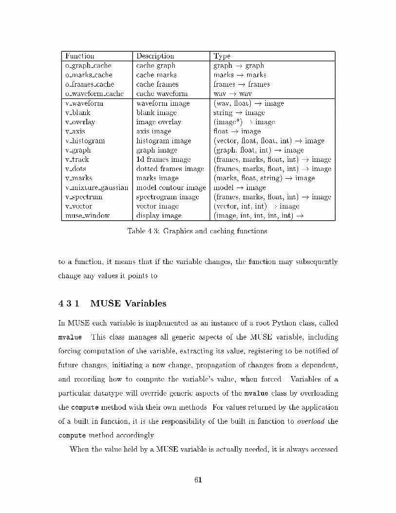
Function Description Type
o graph cache cache graph graph ! graph
o marks cache cache marks marks ! marks
o frames cache cache frames frames ! frameso waveform cache cache waveform wav ! wav
v waveform waveform image (wav, oat) ! image
v blank blank image string ! image
v overlay image overlay (image*) ! imagev axis axis image oat ! image
v histogram histogram image (vector, oat, oat, int) ! imagev graph graph image (graph, oat, int) ! image
v track 1d frames image (frames, marks, oat, int) ! image
v dots dotted frames image (frames, marks, oat, int) ! imagev marks marks image (marks, oat, string) ! image
v mixture gaussian model contour image model ! imagev spectrum spectrogram image (frames, marks, oat, int) ! imagev vector vector image (vector, int, int) ! image
muse window display image (image, int, int, int, int) !
Table 4.3: Graphics and caching functions.
to a function, it means that if the variable changes, the function may subsequently
change any values it points to.
4.3.1 MUSE Variables
In MUSE each variable is implemented as an instance of a root Python class, called
mvalue. This class manages all generic aspects of the MUSE variable, including
forcing computation of the variable, extracting its value, registering to be noti�ed of
future changes, initiating a new change, propagation of changes from a dependent,
and recording how to compute the variable's value, when forced. Variables of a
particular datatype will override generic aspects of the mvalue class by overloading
the compute method with their own methods. For values returned by the application
of a built-in function, it is the responsibility of the built-in function to overload the
compute method accordingly.
When the value held by a MUSE variable is actually needed, it is always accessed
61

file
o_load_waveform
w
o_preemphasis m_mul
0.97
pw
o_window_wav
0.005
m_int
win_num_point
o_hanning
win
o_sync_marks
mks
0.005
v_spectrum
w_wav
o_fft_frames
256
stft
o_db_frames
db_stft tscale height
img
Figure 4-2: The dependency graph corresponding to the MUSE spectrogram program
in Figure 4-1.
The graph is derived by MUSE according to the MUSE program, and is used to propagate
run-time changes and perform on-demand computation using lazy evaluation. The oval
nodes correspond to MUSE variables, while the rectangular nodes correspond to the ap-
plied MUSE built-in functions which establish relationships between the MUSE variables.
According to the program, the variables are named if they had a name in the program; the
blank node near the top corresponds to the unnamed MUSE variable created on line 9 of
Figure 4-1 by the call to m mul.
62

functionally: the force method must be called. In this way, the mvalue class may
either quickly return a pre-cached value or recursively call other functions in order to
generate the value. Most of the time it is the built-in functions that force their input
mvalues in order to perform their computations, but the programmer may also do so.
Of the datatypes supported by the toolkit, some are atomic, meaning their entire
value is computed at once, while others are non-atomic, meaning they support e�cient
random access and are able to compute portions of their value if required. The atomic
types are basic, vector and model. When a MUSE value of one of these types is
forced, the actual value, represented as a Python value, is returned. The non-atomic
types are marks, wav, image, graph and frames. When the force method for a
MUSE value of one of these types is called, a class instance, which obeys the a
functional API corresponding to the datatype, is returned. For example, a variable
of type marks must provide a range method, which returns the integer labels of all
marks falling within a speci�ed time range. The wav type must provide the method
samples which will return a requested range of samples.
Caching
Every MUSE value is aggressively cached, which means the �rst time it is computed,
the value is saved for future reference. When force is called, if the value is already
cached, it will quickly return the cached value. If it is not cached, it will instead call
the compute method of the mvalue, which will return the value. This value is then
cached and returned.
For atomic types, the actual Python value is directly cached and returned when
the MUSE variable is forced. For non-atomic types, it is only the class instance
representing the type that is cached. Therefore, caching of non-atomic types is not
handled automatically by MUSE; instead, a collection of MUSE functions, listed in
Table 4.3 o�er programmer-controlled caching. Functionally, each cache is just the
identity function; however, internally, the cache is storing recently accessed portions
of the datatype. These caches allow the programmer to limit the maximum amount
of space to be used, as they can expand to cache arbitrarily large data structures.
63
For example, the frames cache can be inserted after the o fft frames function, in
order to store the frames in case they are needed in the future. Without a cache,
the frames will be recomputed every time they are needed. Each cache has a policy
speci�c to the datatype. The frames cache will cache individual frames at a time,
and will only compute and cache what its dependents have asked for. However, the
waveform cache is page-based, and will ask for whole pages of its input, in response
to a request from its dependent. Because of the di�culty of e�ective scrolling, there
is no separate image cache function. Rather, it is built into the window function, and,
like all other caches, allows the programmer to control maximum memory usage.
If the programmer creates a constant, atomic value directly by calling mvalue, it
is immediately cached, so that if it is ever forced, that value is returned (because it
cannot ever be recomputed if it is not cached). However, when a built-in function
creates an atomic variable, it does not have to specify the value contained by the
variable, but may instead overload the compute method of the mvalue with its own
method.
Change
Every datatype supports the ability to change, and the mvalue class o�ers generic
methods to register for noti�cation of future change (register, depends), to initiate
a new change by replacement (change) and to forward a change (notify).
MUSE allows two forms of change: replacement and incremental. Replacement
change occurs when the programmer calls the change method of a MUSE variable,
which takes a single argument, the new value, and replaces the current value of the
MUSE variable with the new one. Incremental change is initiated with datatype
speci�c functions. For example, any MUSE variable of type marks must provide the
add mark, del mark and move mark. In both cases, all dependents of the MUSE vari-
able are recursively noti�ed of the change. Dependents may be functions which had
been previously applied to the variable, or callback functions which were registered
with the variable. The noti�cation process is recursive: a function, in responding to
a change, may change its output variables. Also, the callback functions may initiate
64

changes in other MUSE variables as well. The process cascades until no dependents
remain.
With each variable that is noti�ed of a change, two possible actions may occur.
If the variable has a cached value, then the cache is discarded and the change is
forwarded to all dependents. However, if its value is not cached, then nothing hap-
pens: an un-cached value means that nothing has asked for the value and therefore
nothing beyond the value can possibly depend upon it. This is an important opti-
mization for a rapid succession of related changes: the �rst change will recurse all the
way down the dependency graph, clearing caches, but any subsequent changes will
quickly return once they encounter a variable whose cache was cleared by the �rst
change-propagation (as long as it was not recomputed in the interim). However, the
optimization only applies because MUSE never discards a non-atomic cached value,
which future implementations might wish to do. When a change encounters the cache
of a non-atomic datatype, the cache carefully clears out the a�ected portion of the
value, then continues to forward the change to all of its dependents. For example,
when an image changes in a certain rectangular region, the image cache in the window
must erase that rectangular portion from the cache. This increases the complexity of
non-atomic datatype caches.
When a built-in function creates new output variables, it will register them with
the input variables on which they depend, using the depends method of the mvalue
class. When a change subsequently arrives, the built-in function may interpret the
change, and then forward the change to all of its outputs. It is important to note that
during this forwarding, the built-in function will not perform any computation of the
new value. Rather, it must incrementally compute the impact of the changed inputs
on its outputs, which typically is quite a bit less computation than actually computing
the new value. Subsequent computation will only occur if one of the function's output
value is forced through lazy evaluation.
I refer to this model of change propagation as synchronous change propagation.
Although Sapphire's model of change propagation is also synchronous, the changes
allowed in Sapphire are only entire replacement, which greatly simpli�es the propa-
65

gation of change. Because of this, Sapphire is able to recursively mark all dependent
values as \dirty", without consulting the built-in functions that relate and depend
upon each of the impacted variables. In contrast, MUSE consults each built-in func-
tion during change propagation to allow it to assess whether and how a change in its
input should be propagated to a change in its outputs.
4.3.2 Built-in Functions
MUSE built-in functions, once applied, are responsible for maintaining, throughout
the duration of the MUSE program, a functional relationship between their input and
output values. They must compute output values from input values, on demand, and
respond appropriately to any subsequent changes in their inputs values. Each built-in
function is implemented as a Python class, with some extensions in C for computa-
tional e�ciency (e.g., the FFT code in Figure 4-3 imports the sls module, which
is implemented in C); Python makes such extensions very simple. In keeping with
Python's conventions, a MUSE built-in function takes both tuple arguments, which
is just an unnamed list of arguments, and keyword arguments, where each argument
is named (this is similar to Tk). Every time a built-in function is applied, it instanti-
ates the corresponding Python class. Using a Python class instance for each built-in
application allows the built-in to easily retain any necessary internal state re ecting
its current computations. An example built-in function implementation is shown in
Figure 4-3. This function implements the o fft function, which maintains the FFT
of a single input vector, optionally converting the output into decibels (do db) or
inverting it (do invert). All inputs to a built-in function application must be MUSE
values; if the user provided an argument that is not an mvalue instance, a suitable
mvalue will be created (this is the purpose of the clean and dclean functions).
The init method of the built-in function, which is the function called when
the class is instantiated, must perform a number of tasks in order to establish the
function application and prepare for future computation and changes. However, it
does not perform any actual computation of the function it represents; this happens
only in the future, on demand. It must check that the types and number of the input
66

from muse import *
import Numeric, math, sls; npy = Numeric
class _o_fft:
def __init__(self, vec, npoint, do_invert=mvalue(0),do_db=mvalue(1)):
self.vec = vecself.npoint = npointself.do_invert = do_invertself.do_db = do_db
self.out = mvalue()self.out.compute = self.compute
self._fft = None
self.out.depends(self.vec)self.out.depends(self.do_db)self.out.depends(self.do_invert)self.out.depends(self.npoint, self.notify)
def notify(self):self.out.notify()self._fft = None
def compute(self):np = self.npoint.force()doi = self.doinvert.force()dod = self.do_db.force()vec = self.vec.force()
if self._fft == None:self._fft = sls.fft_create(np*2)
ans = Numeric.zeros(np, Numeric.Float32)sls.fft(self._fft, vec, ans)if dod:
sls.transform_db(ans, ans, doi)return ans
def o_fft(*args, **dargs):x = apply(_o_fft, clean(args), dclean(dargs))return x.out
Figure 4-3: Python code implementing the complete o fft built-in function.
The o fft built-in computes the FFT of a vector, optionally inverting the output or con-
verting it to decibels. The function imports the sls module, which is implemented in C,
for actually computing the FFT function.
67

arguments are correct (the Python interpreter performs some of these checks, when
it matches formal and actual function arguments). It must record the input MUSE
values within its class instance so that it may later refer to them. It must express its
dependence on these input values, so that it will be noti�ed if they ever change. It
must create any return values, providing its own functions to compute these values if
they are ever forced.
The built-in function expresses dependency on a particular MUSE value by calling
the depends method of the value. In the example, the output of o fft depends on
all four input values. When calling depends, if there is no second argument, then
the run-time system assumes that any change on this input value means that the
entire output value should just be recomputed. The optional second argument, if
provided, is a function to call, instead. The o fft function provides a function only
if the npoint parameter changes; this is because it has internal state (the internally
cached sine/cosine tables) that must be recomputed if the number of points in the
FFT changes.
The built-in function creates any output values by calling mvalue, which instan-
tiates a new MUSE value instance. The value is then specialized to the built-in
function by overwriting its compute method with a method of the built-in function.
Thus, if in the future this MUSE value is forced, the compute method of the o fft
built-in function will be called. For non-atomic data types, which support a richer
API for accessing the values of the type, the built-in function will provide its own
class instance to the call to mvalue; in this manner, the built-in function implements
the API appropriate for a single output datatype.
When the built-in function is applied in a MUSE program, the only method which
is actually called is the class instance initialization method, init . The function
establishes dependencies and creates return MUSE variables, but performs none of the
actual computation for that built-in function. Instead, when the value of its output
is later needed in the future, its compute method will be called, at which point the
built-in function will force the computation of whatever inputs it needs (this can be
seen in the �rst four lines in the compute method in Figure 4-3, and then proceed to
68
actually compute itself.
The MUSE programmer never directly interacts with the built-in function's class
instance. In fact, the instance is never returned to the programmer; instead, a small
\helper" function, as seen at the bottom of Figure 4-3, instantiates the class and then
returns all output MUSE values for that built-in function. Therefore, the only way to
indirectly interact with the built-in function instance is by changing the input MUSE
values to which the built-in function was applied.
The compute method of the built-in function will be called whenever some function
requires the value of the output of the built-in function. This is where the actual
function's computation takes place. It will then force the computation of any number
of its input values, thereby extracting the values in Python's representation, perform
its computation, and then return its result. In addition, it may also compute and
retain any internal state that it needs for its computation (the o fft function, for
example, �lls in the sine/cosine tables for the FFT by calling sls.fft create). That
force method will frequently result in the calling of the compute method of another
built-in function; the process cascades.
Portions of a built-in function's computation may be implemented in C, for e�-
ciency. For example, the slsmodule, which is imported by the o fft implementation,
is implemented in C, and contains the actual code to compute the FFT. The call to
sls.fft create, sls.fft and sls.transform db are all implemented in C.
Incremental Computation
Many built-in function implementations will choose to take the default approach of
simply redoing their entire computation in response to any change, and for many
functions this is an appropriate choice either because their compute time is negligible
or because the e�ort required to implement incremental computation is prohibitive.
However, several of the built-in functions in this implementation make e�orts to
compute incrementally, because the potential time savings, and therefore impact on
interactivity, is important. The v spectrum function will incrementally change its
output image in response to particular changes in the time marks input. The e�ect
69

is to only change a rectangular portion of the output spectrogram in response to a
changed time-mark. The o word spot function, likewise, will incrementally change
its output graph in response to changes in its input graph. If the user changes the
label of an edge, or adds a new edge, to the existing transcription, the o word spot
function will quickly incrementally compute how the output graph will change.
During incremental computation, each function does not necessarily compute the
change to its output, but rather the bounds of the change. For example, v spectrum
need only translate a change on its input marks to the corresponding rectangular
region of its output image which is a�ected. The actual recomputation of the a�ected
image happens only later, if a window needs to display it. Frequently the propagation
of such bounds of the change requires far less computation than actually computing
the full change.
4.3.3 Integration with Tk
In order to remain interactive, MUSE is integrated with the Tk mainloop function.
The purpose of mainloop is to constantly poll for and respond to user actions. There
are two channels through which MUSE is able to gain control of the single thread of
control running in Python and Tk. The �rst comes through the windows that display
MUSE images. FromTk's point of view, all computation performed by MUSE appears
just like any other Tk widget: the window or windows that display MUSE images to
the user will issue a request for computation at startup or in response to a change
in their image. When Tk has a chance (i.e., after servicing any other requests), it
will visit the window, allowing it to compute and display its image. The window,
in an e�ort to o�er pipelining and remain backgrounded, will only draw a small
portion of what actually needs to be drawn, and then issue another request for later
computation. It does this because during the time when it has the only thread of
control, the rest of the tool will be unresponsive. Tk otherwise calls no other MUSE
functions directly, because the window, through lazy evaluation, will call all other
MUSE functions.
The second way for MUSE to gain control is in response to a GUI event. For
70

example, when the user slides a scrollbar, Tk will call a Python callback function,
which in turn will change the value of a MUSE variable. When that change function
is called, MUSE has control as it recursively calls the change functions of all variables
that depend upon the original variable. Often, that change will eventually reach a
window, and in response, the window will issue a request for later computation from
Tk.
4.3.4 Example Scenario
In order to illustrate the ordering of computations within the toolkit, in this section
I step through the computations taken for the example MUSE program shown in
Figure 4-4 (this is the same example from Figure 4-1, but repeated here for spatial
locality). This program computes a spectrogram image (img) from a waveform stored
in a �le ("input.wav"). The image could then be displayed in a tool containing GUI
widgets that the user may use to change certain aspects of the computation. The
waveform is �rst loaded (w) and then preemphasized (pw), and a Hanning window
(win) is then applied to it, at a frame rate of 5 ms. This results in a set of win-
dowed frames (w wav), which are then passed through the o fft frames to compute
the FFT of each frame (stft), then translated into the dB scale with o db frames
(db stft), and �nally translated into a spectrogram image (img) with v spectrum.
The corresponding dependency graph is shown in Figure 4-2.
When this program is initially executed, no computation towards the image will
actually occur until the window into which the image is displayed becomes mapped
by Tk and the X Window system, making it visible to the user. When the Tk
loop is idle, it will call upon the window to draw itself. The window, because it is
pipelined, will ask img to draw one portion at a time, from left to right, returning
control to Tk after each portion. When the window draws the �rst portion, it will
ask the v spectrum function to produce that part of the image, which will in turn
force the value of tscale, in order to compute what time range this corresponds
to. Next, v spectrum will look up the set of time marks that fall within the time
range. Given this set, it will ask its input frames (the output of o db frames) for the
71

1 w = o_load_waveform("input.wav")
# preemphasized waveform
preem = mvalue(0.97)
5 pw = o_preemphasis(w, preem)
# hanning window (5 msec)
win_dur = mvalue(0.005)
win_num_point = m_int(m_mul(win_dur, wav.force().srate))
10
win = mvalue(o_hanning(win_num_point))
# synchronous marks (5 msec)
frame_dur = mvalue(0.005)
15 mks = o_sync_marks(mvalue(frame_dur))
# windowed waveform frames
w_wav = o_window_wav(pw, win, mks)
20 # fft frames
stft = o_fft_frames(w_wav, mvalue(256))
# fft frames (in decibels)
db_stft = o_db_frames(fft)
25
# spectrogram image
tscale = mvalue(400.0)
height = mvalue(300)
img = v_spectrum(tscale, mks, db_stft, height)
Figure 4-4: MUSE program to compute a spectrogram image from a waveform.
72

frames corresponding to those marks. That function will, in turn, ask o fft frames
frames for its output, which will then ask o window wav for its outputs. Because this
is the �rst time o window wav is being called, it will force the o hanning function to
compute. In turn, o hanning will force m int to compute. Eventually, the Hanning
window is computed and cached (because its output type, vector, is atomic, it will
be aggressively cached), at which point o window wav will look up the times of the
associated marks, and will then ask o preemphasis for a range of waveform samples.
Finally, the o load waveform function will load and return the corresponding samples
from �le.
Even though the function calls are enumerated recursively, from the bottom (win-
dow) up (o load waveform), the net ordering of the computation is actually top
down, according to the dependencies in the graph. The stack trace that is enumer-
ated during this process is a depth-�rst search of the reverse of the dependency graph
representing the MUSE program. During this �rst stage, the stack is growing, with
each function call. As values are returned, the stack shrinks again, as the actual
computations at each stage take place. Eventually, the image portion is returned to
the window, and it will display it on the screen for the user to see.
Tk will eventually call the window again, so that it may continue to draw. When
this happens, the same depth-�rst search will take place, except that certain val-
ues, because they were computed the �rst time around, will be cached, for example
win num point and win. Whenever these values are forced during the computation,
they will return immediately with their value, avoiding redundant computation.
Eventually, the window will have drawn its entire contents, at which point it
will stop requesting computation from Tk. The run-time system will then remain
idle, awaiting actions by the user. Perhaps the user might then change some aspect
of the computation, for example the time-scale input (tscale) to the v spectrum
function. In response to this change, v spectrum will notify its image output that it
has changed, in entirety. In response to this, muse window will redraw the spectrogram
image again. Note that this will cause the waveform to be reloaded and the STFT
to be recomputed, despite the fact that they have not changed (only tscale did).
73

This could be easily recti�ed by inserting a frames cache, using o frames cache, right
after the computation of o db frames, in order to cache the value of db stft.
Perhaps we would like to allow the tool user to alter individual frames of the short-
time Fourier transform. In order to do this, we would need to use o marks cache
to hold the output of o sync marks, and then provide appropriate GUI bindings
allowing the user to delete or move existing time marks and to add new ones. With
each change, the cached marks would alter the corresponding value, and notify its
output dependents. For example, if a new time mark is added, both o window wav and
v spectrum will be noti�ed of the change. o window wav will interpret the change by
notifying the output frames that a new frame has been added, but it will not compute
that value. That change will be forwarded to o fft frames and on to o db frames.
v spectrum will actually ignore the change because it knows it will also be noti�ed of
such changes through the marks (however, it will pay attention to other changes that,
for example, could have originated in the FFT computation). It therefore returns,
all the way back to the marks cache, which now noti�es v spectrum directly. In
response to this change, v spectrum will compute the impact of adding a time mark
on its output image, by calculating the rectangular sub-region that will be replaced.
During the change propagation, v spectrum will force the value of tscale in order
to compute the impacted region of its output image, however the new image is not
actually computed. Instead, any functions, for example a window that is displaying
the image, that rely on the image value are noti�ed of the change. The window, if
this rectangular region is in view (which it most often is) will make note of the fact
that it needs to redraw this portion and request later computation from Tk.
When the window is later scheduled to redraw, it will go through the same
pipelined process that it did at startup. This will cause only the FFT corresponding
to the newly added mark to be computed (assuming the frames cache has stored
everything else), and the new portion of the image to be drawn.
74

4.4 Summary
MUSE presents to the programmer an abstract form of expression that integrates large
and small datatypes and functions. The programmer is able to establish functional
relationships among variables and initiate changes to variables, without concern as
to the details of how the computation should be executed. By providing explicit
caches, MUSE gives the programmer exibility to control memory usage. At run-
time, MUSE studies the program, creates the corresponding dependency graph, and
then selects an interactive approach for executing the tool. While there are many
possible techniques for implementing MUSE's architecture, this thesis explores one.
In the next chapter I evaluate the resulting interactivity of MUSE.
75

Chapter 5
Evaluation
In this chapter I evaluate the success of MUSE in achieving the stated goals of this
thesis. In particular, I wish to assess the interactivity of MUSE tools. The evaluation
is two-fold, re ecting the properties of MUSE. First, MUSE enables new forms of
interactivity which are not currently available in other speech toolkits. Examples of
this include \editing" a spectrogram, incremental lexical access and interaction with
arbitrarily long utterances. Because this functionality is novel, and therefore not
easily compared with existing toolkits, I will describe a set of example MUSE tools
and argue subjectively that their novel functionality is also valuable.
Second, MUSE o�ers improved interactivity for existing functionality. In order
to demonstrate this, I compare MUSE to Sapphire with respect to the six proposed
metrics for interactivity. Sapphire was selected because it one of the more interac-
tive of existing toolkits (see Chapter 3), and its source code was readily available for
extension with pro�ling and user simulation code. I design a speech analysis tool,
implement it in both MUSE and Sapphire, and measure the resulting interactivity of
each. When possible, I present actual measurements of interactivity, such as average
response time and net memory usage. Otherwise, I o�er my subjective evaluation
based on my experiences interacting with the example tools and knowledge of both
toolkits. The next chapter will discuss the strengths and weaknesses of MUSE re-
vealed by this evaluation, suggest directions for future work and conclude the thesis.
76
5.1 Example MUSE Tools
Using MUSE I have created various example tools that demonstrate its unique capa-
bilities. I have selected �ve such tools, described here. However, many other tools are
possible; these were selected in order to demonstrate MUSE's novel characteristics
and the e�ectiveness of the MUSE architecture.
What is novel about these tools is the high degree of interactivity o�ered to the
user, typically through a continuous interface supporting changes in many parameters.
Each tool presents a control panel allowing many aspects of the computation to be
continuously changed, and gives corresponding continuous feedback. Novel forms
of functionality, such as the editable spectrogram and incremental lexical access,
are made possible by MUSE's incremental computation model. Such functionality is
important as it allows researchers to ask questions and explore approaches which they
are currently unable to do, and can therefore potentially lead to future breakthroughs
in our approaches to speech understanding. Furthermore, although this has not been
formally tested, I believe the tools as they now stand would make excellent educational
aides in a speech recognition course.
5.1.1 Speech Analysis
This tool, shown in Figure 5-1, is a basic speech analysis tool. From top down, the
user sees the low-frequency energy, the spectrogram, the waveform, the phonetic tran-
scription, the orthographic transcription, and a time axis. In a separate window is
a control panel allowing the user to directly manipulate many of the underlying pa-
rameters, including the time-scale, frame rate, analysis window and duration. When
the time-scale is \zoomed in" enough, overlaid time marks appear on the waveform,
indicating the alignment of the individual STFT frames used to compute the spectro-
gram image. Using the mouse, the user is able to edit these time marks, by adding
new ones and deleting or moving existing ones. With each edit, the impact on the
spectrogram is quickly computed and displayed to the user. The user is then able to
see the impact of di�erent STFT frame alignments on the spectrogram image. For
77

example, in Figure 5-1, the portion of the spectrogram between 0.8 and 0.9 seconds
has been edited to be pitch synchronous. Figure 5-2 shows a series of screen snapshots
as the user drags one of the time marks.
Being able to \edit" a spectrogram makes it clear that the spectrogram, as re-
searchers now think of it, is not a �xed, decided signal representation, but is in fact
subject to further modi�cation and exploration. This gives us the power to question
the representation and perhaps improve upon it. For example, the pitch synchronous
spectrogram looks, subjectively, better than the corresponding �xed frame-rate spec-
trogram which uses the same number of parameters. Further, by setting the frame
period to 5 or 10 ms and the window duration to 25 ms, the researcher is able to
see the rather ugly and information-losing representation used by modern speech un-
derstanding systems. In contrast, a relatively short frame period and analysis look
much better. By sliding the scale controlling the frame period, the user can view
the curious interaction between frame period and pitch period. Pitch-synchronous
analysis may improve the performance and accuracy of future speech understanding
systems, and tools which allow researchers to visualize the e�ect represent the �rst
step towards building such systems in the future. This functionality is made possible
by MUSE's incremental computation: as each time mark is added, moved or deleted,
MUSE propagates the incremental change to the spectrogram image. As a conse-
quence, only a certain rectangular portion of the image will be recomputed, enabling
the continuous response.
5.1.2 Mixture Diagonal Gaussian Training
This example tool, shown in Figure 5-3, exposes the computations for training a
one-dimensional Gaussian mixture model. The data is either synthetically generated
according to a mixture of one, two or three Gaussians, or is the log-duration of one
of the 61 standard TIMIT phones (from the standard TIMIT training set). The user
is able to select the data source, and vary the number of data tokens using a scale.
Training consists of randomly seeding the K-Means algorithm, running K-Means
for some number of iterations [7], then running the EM algorithm for some number of
78

Figure 5-1: A spectrogram editor.
From the top down, the user sees the low-frequency energy display, the spectrogram, the
waveform, the phonetic transcription and the orthographic transcription. A separate win-
dow presents scales allowing the user to change many of the underlying parameters through
direct manipulation. By zooming in, the user may edit the time marks representing the
alignments of individual STFT frames, thereby interactively \editing" the spectrogram im-
age. Using this tool, a student could visualize the impact of a pitch synchronous spectrogram
in comparison to the representation used by modern speech understanding systems. For
example, the spectrogram around 0.8 to 0.9 seconds in the word \we" has been edited in
such a fashion.
79
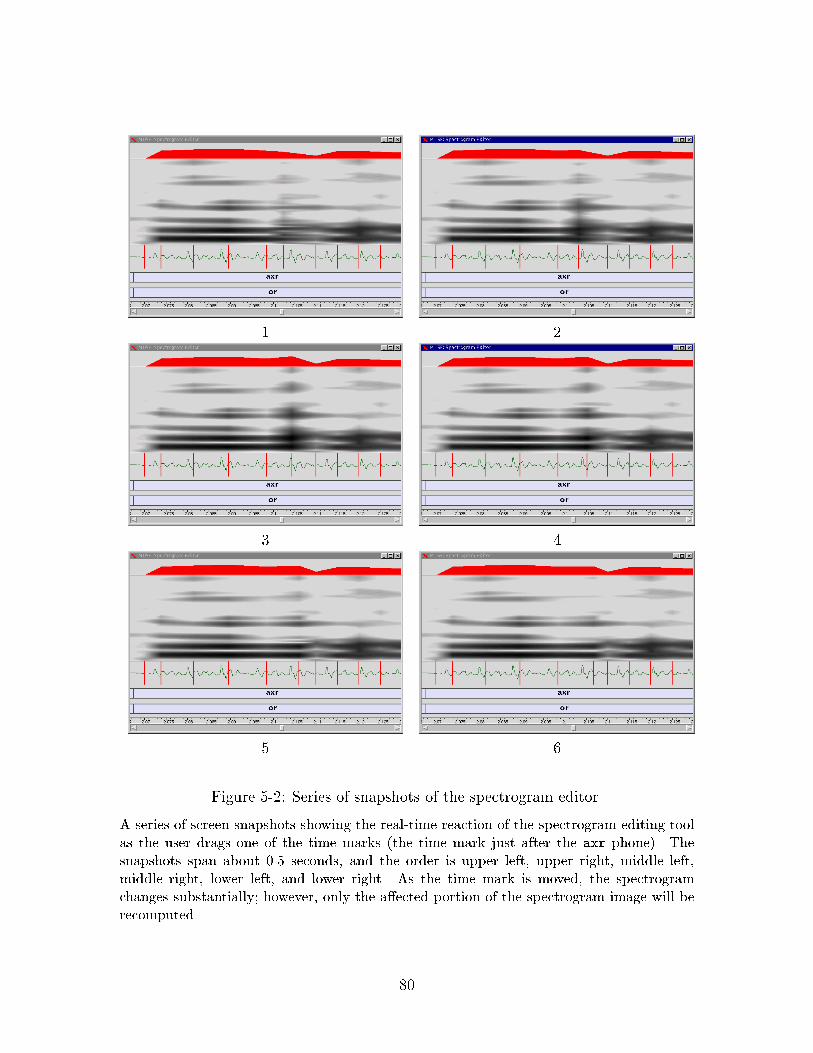
1 2
3 4
5 6
Figure 5-2: Series of snapshots of the spectrogram editor.
A series of screen snapshots showing the real-time reaction of the spectrogram editing tool
as the user drags one of the time marks (the time mark just after the axr phone). The
snapshots span about 0.5 seconds, and the order is upper left, upper right, middle left,
middle right, lower left, and lower right. As the time mark is moved, the spectrogram
changes substantially; however, only the a�ected portion of the spectrogram image will be
recomputed.
80

iterations [33], �nally producing the trained mixtures. The tool displays a histogram
of the data, whose bin size the user can change, with the trained mixture model
(both the individual kernels and the combined mixture model) overlaid, along with
the per-token log-likelihood of the data. The user is able to change many aspects
of this computation and see continuous feedback, including the number of mixtures,
data source, amount of data (for the synthetic data sources), number of iterations of
K-Means and of EM, and number of bins in the histogram. Buttons allow the user
to re-sample the data (for synthetic data), and to re-seed the K-Means algorithm.
The continuous interface allows the user to visualize each iteration of K-Means
and EM, by sliding a scale, as well as the di�erences between how the two algorithms
evolve the mixture kernels. The user is able to explore many important aspects of
models training, such as the impact of sparse data and over-�tting, the e�ectiveness
and di�erence between K-Means and EM, the impact of number of mixtures versus the
data source characteristics, e�ectiveness of the trained mixtures with the underlying
mixtures, the e�ect of random initial seeding, etc. Figure 5-4 shows the series of
images resulting from continuously changing the number of K-Means iterations, while
Figure 5-5 shows the images resulting from continuously changing the number of EM
iterations. Training of the Gaussian mixture models is known to be one of the di�cult
and limited areas of our speech recognition system [14]; tools such as this one may
expose important opportunities to students and researchers.
5.1.3 Lexical Analysis
This tool, shown in Figures 5-6 and 5-7, illustrates the lexical-access or search stage
of speech recognition, and can serve as a useful aid to a student learning how to read
spectrograms. The user sees a waveform and spectrogram, and two initially blank
windows. In the �rst window the user is able to interactively transcribe the utterance
as a phone graph, expressing alternative segmentations, using the mouse to place
boundaries and edges, and the keyboard to label the edges. When labelling each edge
of the phone graph, the user may use broad classes such as vwl for any vowel and nsl
for any nasal (the user can easily de�ne classes), or just list a sequence of possible la-
81

Figure 5-3: An interactive one-dimensional Gaussian mixture training tool.
The tool uses the K-Means and EM algorithms to train a one-dimensional Gaussian mixture
model, and presents three windows to the user. The top window displays a histogram of the
data, with the trained model overlaid (both the Gaussian kernels and the mixture model),
as well as the net log-likelihood (in the lower right corner of the top window) of the data
according to the trained model. The second window allows the user to choose the source
of data, either one of three synthetically generated sources (according to one, two or three
Gaussian mixtures, respectively), or the log-duration of any of the standard 61 TIMIT
phones across the TIMIT training set [11]. The third window allows the user to vary many
of the parameters controlling the training, and receive a continuous real-time response. The
tool allows the user to understand many important aspects of training, such as sparse data
and over-�tting, the di�erence between K-Means and EM, the impact of random initial
seeding, and the convergence properties of the training algorithms.
82

1 2
3 4
5 6
Figure 5-4: Series of snapshots of the Gaussian mixture tool.
The snapshots show the continuous response to the user's direct manipulations when chang-
ing the number of iterations of the K-Means algorithm from 0 to 9, and the number of
iterations of EM �xed at 0. The starting image corresponds to a Gaussian mixture model
trained from seeds only (no iterations of K-Means nor EM). After 9 iterations the K-Means
algorithm has converged. The log-probability assigned to the data by the model correspond-
ingly improves from -2.07 to -1.992; furthermore, the K-Means algorithm, for this number
of mixtures and particular data source, fails to converge to the actual underlying mixtures.
In real-time, the snapshots span about 0.5 seconds, and the order is upper left, upper right,
middle left, middle right, lower left, and lower right.
83

1 2
3 4
5 6
Figure 5-5: Series of snapshots of the Gaussian mixture tool.
The snapshots show the continuous response to the user's direct manipulations when chang-
ing the number of iterations of the EM algorithm from 0 to 10, with the number of iterations
of K-Means �xed at 9. The starting image is the �nal image from Figure 5-4, with 9 it-
erations of K-Means and 0 iterations of EM. After 10 iterations, the EM algorithm has
converged. The log-probability assigned to the data by the model correspondingly improves
from -1.992 to -1.860; the EM algorithm is able to more e�ectively converge to the under-
lying mixtures. In real-time, the snapshots span about 0.5 seconds, and the order is upper
left, upper right, middle left, middle right, lower left, and lower right.
84

bels. As the user creates the transcription, the second window displays, continuously,
a graph of word matches. By continuously seeing which words match where, the user
is able to gain feedback and perhaps alter the transcription accordingly. When a
correct word appears (the tool has as input the correct orthographic transcription) it
will be highlighted in green.1 Another window shows the zoomed-in waveform with
editable time marks overlaid, and allows the user to \edit" the spectrogram, as in the
tool from Section 5.1.1, to get a clearer picture of formant motion during transitions,
for example.
Incremental lexical access generalizes the search stage of speech recognition, which
is normally \left to right" and not amenable to interaction. The tool is an excellent ed-
ucational aid for illustrating important properties of lexical access, as well as learning
how to read spectrograms. It allows students to explore the strengths and weaknesses
of potential alternative forms of lexical access such as island driven approaches; these
alternatives are di�cult to explore now. It also gives students an appreciation of
the search process, as they can learn which sounds best serve to initially constrain
possible word matches. The importance of some form of pronunciation modeling,
which serves to match the phones used for recognition with the phonemes used for
the lexicon, becomes painfully clear with this tool: without such rules, lexical access
is very di�cult. This tool is made possible by MUSE's incremental computation: in
response to each change made by the user to the phone graph, the lexical access func-
tion incrementally propagates the change to the output word graph, thus allowing a
continuous and real-time response.
5.1.4 Spectral Slices
This tool, shown in Figures 5-8 and 5-9, compares several di�erent spectral representa-
tions: the standard Fourier transform [34], the LPC-spectrum [34], and the cepstrally
smoothed spectrum (low-pass liftering) [28]. There are four displays. The �rst shows
a zoomed-in waveform view with a time mark and analysis window overlaid; the time
1This is very rewarding feedback.
85

Figure 5-6: An interactive lexical-access tool.
The tool shows, from top down, the low-frequency energy, the spectrogram, the waveform,
a time axis, the user's phonetic transcription, and the matching word transcription. As
the user phonetically transcribes the speech in any order (i.e., not just \left to right"),
he or she is presented with the continuously matching word alignments from the TIMIT
lexicon [11]. Broad classes, such as stp (which represents p, t, k, b, d and g), may be
pre-de�ned and used during transcription. The tool is useful as an aid when learning to
read spectrograms, and also as an educational tool to understand the properties of lexical
access. A zoomed-in waveform view (not shown) allows careful study of the waveform and
editing of the spectrogram.
86

1 2
3 4
Figure 5-7: Series of snapshots of the lexical access tool.
The snapshots illustrate the incremental, interactive nature of the tool. The tool allows the
user to phonetically transcribe the utterance in any order; with each segment added or label
changed, the matching words are continuously updated below. In response to the matched
words, the user may interactively alter the phonetic transcription, completing the feedback
process. The tool is con�gured to highlight \correct" words in green.
87

mark, which tracks the user's mouse when it is in the window, is the point where the
spectral analysis is computed. The second window shows the windowed waveform.
The third window shows the overlaid spectral slices. The fourth window is a control
panel with scales and buttons.
As the user moves the time mark, all displays are updated accordingly. Using
checkbuttons, the user can select which spectral slices should be overlaid, as well
as which analysis window should be used. The user can easily vary, using sliders,
parameters such as the LPC order, the cepstral order (cuto� of the low-pass lifter),
the duration of the analysis window, and the time-scale. With each change, the user
receives continuous and real-time feedback.
Such a tool is very useful to teach students the properties, tradeo�s and di�erences
among the various choices for signal representation during speech recognition. For
example, the user can explore the impact of LPC order, window type and duration,
and pitch alignment, on the LPC spectrum, or she could compare the di�erence in
�t between the LPC spectrum and the FFT, and the cepstrally smoothed spectrum
and the FFT.
5.1.5 Long Utterance Browser
This tool, shown in Figure 5-10, is an example of how MUSE enables users to interact
with extremely long utterances (tested up to a 30 minute Broadcast News [10] utter-
ance). With such utterances, the normal scrolling model becomes ine�ective because
a single pixel motion in the scrollbar corresponds to more than a page's worth of the
scrolled image. Therefore, the tool adopts a di�erent model, where the user is able to
scroll through a transcription of the entire utterance, at a low (pixels per second) time
scale, and then drag a time mark, overlaid onto the transcription, which corresponds
to where the spectrogram and waveform images are centered.
A control panel allows the user to change many aspects of the spectrogram com-
putation and display. The waveform image, which is at a higher time-scale than the
spectrogram, is centered by placing the mouse cursor over the spectrogram window.
The time marks overlaid onto the waveform allow the user to edit the spectrogram.
88

Figure 5-8: An interactive FFT, LPC and Cepstrum spectral slice tool.
The top-left window shows three spectral slices overlaid: the standard FFT, on LPC spec-
trum and a cepstrally smoothed spectrum. The top-right window shows the windowed
waveform. The middle window shows the zoomed-in waveform, with the time mark (corre-
sponding to the analysis time) and analysis window overlaid, in addition to the phonetic and
orthographic transcriptions and a time axis. Finally, the bottom window presents a control
panel allowing the user, through direct manipulation, to alter many of the parameters of
the computations underlying the tool, and receive a continuous, real-time response. The
tool allows the user to compare and evaluate many issues related to signal representation
for speech recognition.
89
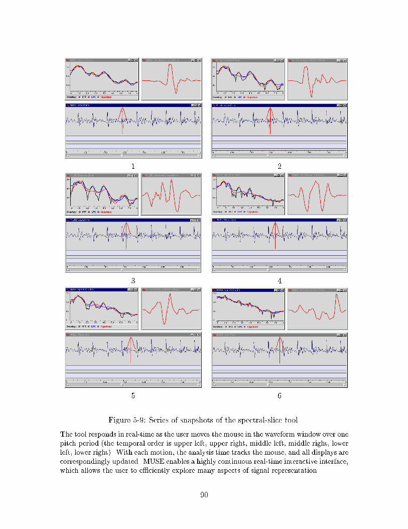
1 2
3 4
5 6
Figure 5-9: Series of snapshots of the spectral-slice tool.
The tool responds in real-time as the user moves the mouse in the waveform window over one
pitch period (the temporal order is upper left, upper right, middle left, middle right, lower
left, lower right). With each motion, the analysis time tracks the mouse, and all displays are
correspondingly updated. MUSE enables a highly continuous real-time interactive interface,
which allows the user to e�ciently explore many aspects of signal representation.
90

This interface allows the user to e�ectively browse very long utterances, which is
infeasible with existing speech toolkits due to computational limitations. Browsing
such utterances is an excellent test of how e�ectively MUSE separates computation
and storage; any function which illegally allocates space can quickly exhaust the com-
puter's resources. For example, the 30 minute waveform alone would require 54 MB
of storage if loaded into memory at the same time.
This functionality is made possible by MUSE's explicit caching model, which
leaves the control of time/space tradeo�s to the programmer: by inserting caches
in appropriate places, and controlling the maximum allowed size of these caches,
the programmer can easily trade o� time and memory usage, as well as limit the
maximum amount of memory used regardless of utterance duration.
Browsing very large utterances in a truly scalable manner allows researchers to
e�ectively study utterances from modern speech corpora. Current approaches to such
browsing require breaking the long utterance into arbitrary chunks, perhaps 10 or 20
seconds is length. This is extra time and e�ort on the researchers part, and the chunks
do not necessarily correspond to natural breakpoints in the utterance.
5.2 Objective Evaluation
In this section I evaluate both MUSE and Sapphire with respect to the six proposed
metrics for interactivity: high-coverage, rapid response, pipelining, backgrounding,
adaptability and scalability. To facilitate direct comparison between MUSE and Sap-
phire, I have designed a common speech analysis tool, shown in Figure 5-11, and
implemented the same tool within both MUSE and Sapphire. The two implementa-
tions are as identical as possible, matching all parameters of the computation, size of
the windows, etc. This tool serves as the basis of an objective comparison between
MUSE and Sapphire, when possible. Otherwise, I o�er my subjective evaluation of
the two toolkits, drawing on some of the example tools from the previous section.
As described in Section 3.6, because Sapphire is the most interactive of the existing
speech toolkits, I only directly compare MUSE to Sapphire.
91

Figure 5-10: An interactive tool allowing browsing of very long utterances.
The standard scrolling model becomes ine�ective for such long utterances, as one pixel of
motion in the scrollbar may correspond to more than a page of motion in the scrolled image.
To compensate, this tool allows the user to scroll through a zoomed out transcription,
and then drag a time mark overlaid on the transcription. As the time-mark moves, the
spectrogram changes its view, continuously. The zoomed-in waveform view with overlaid
time marks allows the user to edit the spectrogram, and the control panel allows the user
to change many aspects of the computation.
92
The speech analysis tool displays a spectrogram, waveform, phone transcription
and orthographic transcription, and allows the user to scroll the images and change
many aspects of the computation, including the analysis window duration, frame
period, time scale, and max-level and range of the spectrogram display. As the user
slides each of these scales, the corresponding image is continuously updated.
5.2.1 Methodology
In order to extract necessary measurements, both MUSE and Sapphire have been aug-
mented to include an \auto-pilot" which simulates a simple user interaction, as well
as a \pro�ler", to extract and log detailed information as to when particular changes
took place, when portions of the response were delivered, and how much memory is
in-use. Each experiment runs the tool under a simulated user interaction scenario,
which consists of a �xed number of change/response iterations of the particular action
being tested. At each iteration, a particular action is taken (by changing the value
being tested), and then the simulation waits until the entire response to the change
is delivered by the tool. For example, when measuring the tool's response to changes
in the analysis window duration, as a function of scroll position, each iteration will
�rst scroll to a randomly chosen location, change the analysis window duration to a
new value, then wait for the complete response. The pro�ling code added to MUSE
and Sapphire results in the creation of a detailed log-�le of the scenario; the log-�le is
subsequently analyzed to extract necessary information. Before the iterations begin,
both tools are �rst thoroughly \pre-cached," by allowing each to scroll incrementally
through the entire waveform, to avoid measuring startup transients.
All experiments were performed on a single computer (an IBM ThinkPad 770)
and operating system (Redhat Linux [35]). The processor is a 233 Mhz Intel Pentium
MMX processor with 96 MB of memory. The windowing system is the Accelerated
X11R6 Windowing system by Xi Graphics; both MUSE and Sapphire were con�gured
to \synchronize" all X functions. Version 1.5 of Python is used. While the tool is
running, it is left \exposed", above all other windows, and no other user-processes
are running (e.g., Emacs, Netscape, etc.).
93

Figure 5-11: The speech analysis tool used to evaluate the interactivity of MUSE and
Sapphire.
The same tool is implemented in both Sapphire and MUSE, for comparison. This �gure
shows the MUSE tool, but the Sapphire tool is identical in all respects.
94
Two quantities are extracted from the log-�le. The average response time mea-
sures how long the tool takes to respond to a particular change, but also takes pipelin-
ing into account. The point of both pipelining and rapid response is to give as much of
the answer to the user, as quickly as possible. The images in each tool, of which there
are four (spectrogram, waveform, phonetic transcription and orthographic transcrip-
tion), are assigned a percentage weight according to the portion of the tool's total
area (measured in pixels) they represent. The spectrogram is 69.77%, the waveform
is 11.63%, and each of the transcriptions is 9.30%. When the tool delivers a pipelined
response to a change, both the delay time of each response and the pixel percentage of
the portion is measured. For example, if the spectrogram image is updated in three
equal pieces, at di�erent times, each time is weighted by 1
3. These response times
are then weighted by the image's pixel percentage to obtain the net average response
time, measured in milli-seconds, to a particular change.
The net memory usage measures how much RAM is allocated by the tool. This
quantity is computed by adding the size of the virtual memory image, as reported by
Linux's Kernel, to any memory allocated as graphics bu�ers (called Pixmaps for X
Windows) on the X Server. This is necessary because under X, Pixmaps are allocated
on the server, under a di�erent process.
5.2.2 High Coverage
High coverage means that an interactive tool o�ers to its user the ability to change
a large number of values impacting the back-end computation of the tool; with high
coverage, the user's explorations are limited by his or her imagination and not by the
tool or toolkit.
High coverage is not easily measured objectively. However, in the speech analysis
tool and in each of the example tools from Section 5.1, high coverage is manifested by
the large number of sliders, buttons, and mouse-event bindings to which each tool is
able to respond. The Gaussian mixture tool, for example, allows the user to change
the data-source, number of K-Means and EM iterations, number of mixtures, and seed
mixtures. While there are elements which are not changeable, for example the precise
95

seed values or the means and variances of the synthetic data, these are limitations
only of that particular tool. With an appropriate interface and a few modi�cations,
these values could easily be made to be changeable by the tool's user. In addition,
MUSE's high coverage is a source of the fundamentally new forms of interaction of
the example tools described in Section 5.1: most of the novel functionality stems from
allowing users to change things which in existing tools are considered immutable, for
example the time marks leading to a spectrogram image.
MUSE tools naturally inherit high coverage from the MUSE architecture, which
explicitly allows any MUSE variable to change, according to the allowed incremental
changes of its datatype, at any moment of time. When building an interactive tool,
the incremental cost to the programmer to o�er the user the ability to change a
certain value is quite low and consists only of connecting an interface component to
the corresponding MUSE variable.
One limitation of high-coverage stems from the granularity of the built-in functions
and datatypes in the speech toolkit. In particular, any values which are used entirely
internally to a built-in function, because they are not exposed as MUSE values, will
not be changeable (unless the built-in function provides access to the value as either
an input or an output parameter). Thus, the extent of high coverage is in general
gated by what MUSE variables are exposed in the toolkit.
Sapphire also o�ers fairly high coverage, in that values may be changed at run-
time. However, such change is not incremental: whole values must be replaced and
subsequently recomputed. Furthermore, because MUSE functions expose a �ner level
of functionality than Sapphire's objects, MUSE exposes certain intermediate values
as directly changeable while in Sapphire these values are hidden.
5.2.3 Rapid Response
Rapid response means that in response to a change initiated by the tool's user, a tool
will subsequently present the impact of the change in a short amount of time. This is
a crucial aspect of interactivity because with such quick feedback to his or her actions,
a user is able to more e�ciently and e�ectively explore the space of possibilities.
96
In order to measure the e�ectiveness of the MUSE model in o�ering a rapid
response, I measure the average response time of MUSE and Sapphire to a change in
three di�erent variables. For each experiment, a 15 second Marketplace utterance is
loaded into the speech analysis tool.
First I measure the response time to scrolling, as shown in Figures 5-12 (MUSE)
and 5-13 (Sapphire). At each iteration, a random scroll position is chosen, the tool is
scrolled (by e�ectively moving the scrollbar to that position, as if the user had done
so), and the complete resulting response time is measured. For each graph, 1000
independent change/response scroll iterations were executed. The x-axis shows the
scroll position in seconds, and the y-axis shows the average response time (in milli-
seconds). The overall average response time is 18.7 milli-seconds for MUSE, and 29.6
milli-seconds for Sapphire, and neither demonstrated a signi�cant correlation with
scroll position. While MUSE is quite a bit faster, both of these results represent a
very rapid response.
Scrolling, because it is a frequent form of interaction, is well handled by both tools,
as re ected by the rapid response time. In order to test a more signi�cant change,
I next measure the average response time due to a change in the analysis window
duration. Each such change requires recomputing both the STFT and spectrogram
image. At each iteration, the tool was �rst scrolled to a particular view, and then
the window duration was changed, and the resulting response time was measured.
Figures 5-14 (MUSE) and 5-15 (Sapphire) show the average response time as a func-
tion of scroll position. Sapphire's response time linearly degrades as a function of the
scroll position, whereas MUSE's response time does not appreciably alter with scroll
position. Because of this property, unless the user is scrolled to near the beginning
of the utterance, Sapphire does not present an e�ective continuous interface to the
user.
As a �nal response time test, I measured response time due to a change in the
time-scale. Changing time-scale requires redrawing the spectrogram image, but not
recomputation of the STFT, and is therefore in general faster than changing the
window duration. At each iteration, the tool was scrolled to a randomly chosen view,
97

0 2 4 6 8 10 12 14 1610
15
20
25
30
35
40
45
50
Utterance Duration (sec)
Ave
rage
Res
pons
e T
ime
(mse
c)
MUSE Scrolling Response Time
Figure 5-12: Average response time for 1000 scrolling trials for MUSE.
Each trial chooses a random point in the 15-second utterance to scroll to, scrolls, and
measures the resulting average response time. The overall average is 18.7 msec. The
periodicity is due to MUSE's image cache: scrolling may require copying portions of either
2 or 3 o�-screen pixmaps, depending on scroll position.
98

0 5 10 1520
25
30
35
40
45
Scroll Position (sec)
Ave
rage
Res
pons
e T
ime
(mse
c)
SAPPHIRE Scrolling Response Time
Figure 5-13: Average response time for 1000 scrolling trials for Sapphire.
Each trial chooses a random point in the 15-second utterance to scroll to, scrolls, and
measures the resulting average response time. The overall average is 29.6 msec. The tail
on the right side of the graph is due to the fact that Sapphire is slightly more e�cient than
MUSE when the user scrolls beyond the end of the utterance.
99

0 2 4 6 8 10 12 14360
380
400
420
440
460
480
500
Scrolled Position (sec)
Avg
. Res
pons
e T
ime
(ms)
MUSE Window Duration Response Time
Figure 5-14: Average response time for 500 trials changing the window duration for
MUSE.
The response time is rather noisy, but does not vary appreciably with scroll position, because
only the portion of the image which the user is currently looking at will be computed. The
mean response time is 406 msec.
100
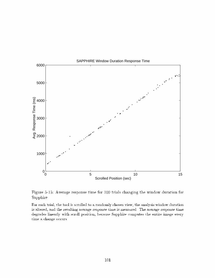
0 5 10 150
1000
2000
3000
4000
5000
6000
Scrolled Position (sec)
Avg
. Res
pons
e T
ime
(ms)
SAPPHIRE Window Duration Response Time
Figure 5-15: Average response time for 100 trials changing the window duration for
Sapphire.
For each trial, the tool is scrolled to a randomly chosen view, the analysis window duration
is altered, and the resulting average response time is measured. The average response time
degrades linearly with scroll position, because Sapphire computes the entire image every
time a change occurs.
101

0 5 10 15180
200
220
240
260
280
300
Scroll Position (sec)
Ave
rage
Res
pons
e T
ime
(mse
c)MUSE Time−Scale Response Time
Figure 5-16: Average response time for 1000 trials changing the time-scale for MUSE.
The mean response time is 205 msec, and does not vary appreciably with scroll position.
and the time scale was changed. Figures 5-16 (MUSE) and 5-17 (Sapphire) show
the average response time. Again, Sapphire degrades linearly with scroll position,
whereas MUSE does not appreciably vary. The average response time for MUSE is
205 milli-seconds, which is quite a bit faster than the average of 406 milli-seconds
when changing the analysis window duration.
5.2.4 Pipelining
Pipelining refers to the process of delivering the answer to a user's question one part
at a time, spread out over time. This is an important quality of interactivity because
102

0 5 10 15500
1000
1500
2000
2500
3000
3500
Scrolled Position (sec)
Res
pons
e T
ime
(mse
c)
SAPPHIRE Time Scale Response Time
Figure 5-17: Average response time for 500 trials changing the time-scale for Sapphire.
The response time, which clearly degrades linearly with scroll position, is distinctly bimodal.
This stems from the fact that the time-scale was changed between 700.0 and 800.0; for
a given utterance position, at the larger time-scale, Sapphire will take longer to draw.
This indicates that Sapphire's response time also degrades with time-scale in addition to
utterance position.
103

when there is a computation which may take a long time, it is important to give the
user partial or incremental feedback. For example, based on this partial feedback,
the user may be able to make a decision or formulate a new question. The average
response time measure already takes pipelining into account by averaging the delivery
times of each portions of an answer.
Pipelining is di�cult to evaluate objectively, so I measure it subjectively here. I
distinguish two forms of pipelining: spatial and temporal. Spatial pipelining refers to
the process of delivering a large image in small, but complete, fragments over time,
while temporal pipelining refers to the process of progressively redrawing the same
area over and over with higher �delity at each step2.
Both MUSE and Sapphire e�ectively demonstrate spatial pipelining as can be seen
by the incremental delivery of the compute-intensive spectrogram image. Spectro-
grams are especially amenable to such pipelining because the amount of computation
scales linearly with the size of the image portion being drawn. Unfortunately, the
computation required for many interactive tools do not exhibit this property. For
example, in the K-Means tool from Section 5.1.2, the primary window displays the
histogram with the trained model overlaid. For this image, the linear correlation
between image area and computation is not present: in order to draw even a small
part of the image, the computer must do nearly the same amount of computation
required to draw the entire image, because most of the computation is spent train-
ing the Gaussian mixture which leads to the image. However, temporal pipelining
is clearly particularly applicable, as K-Means and EM are iterative algorithms, with
each iteration being a closer approximation to the �nal outcome.
Because of the lazy evaluation computation model, MUSE lacks the ability to
perform temporal pipelining: every computation must be completed in entirety be-
fore the function returns. This shortcoming becomes especially noticeable when the
number of mixtures and data tokens is set to a high value: the tool can take a very
long time to update. In contrast, while Sapphire currently does not o�er temporal
pipelining, extending it to do so would be possible. Generalized pipelining is one of
2This is the form of pipelining used by the progressive JPEG and interlaced GIF standards.
104

MUSE's limitations, and will be discussed more in Chapter 7.
Sapphire, because it uses a centralized computation model, supports more general
pipelining than MUSE. In particular, all objects in Sapphire are able to pipeline
their computations, while in MUSE, only the muse window function pipelines. While
currently no Sapphire function exhibits temporal pipelining, incorporating temporal
pipelining into Sapphire would be easier than it would be with MUSE. This has
implications for MUSE's and Sapphire's scalability, as discussed in Section 5.2.6 and
in Chapter 7.
5.2.5 Backgrounding
Backgrounding refers to whether the tool allows the user to pose another question,
even while it is busy computing the answer to a previous question. Of course, just
allowing the user to pose the question is not enough: the tool should also answer the
new question, with a short average response time, as well. Backgrounding is di�cult
to implement because the numerous simultaneous questions may interfere with one
another in complex ways.
The extent of backgrounding is also di�cult to measure objectively, but is sub-
jectively clear based on interactions with the tools. For both MUSE and Sapphire,
backgrounding is tied to pipelining, because they are both implemented in the same
fashion. Therefore, for the speech analysis tool, the extent of backgrounding is,
subjectively, su�cient. For example, when I change the window duration, the new
spectrogram begins to draw. While it is drawing, and before it �nishes, I easily can
change the window duration again, and again. I can also scroll the image around, as
it is being recomputed.
However, the Gaussian mixture tool running under MUSE clearly fails to back-
ground. This only becomes noticeable when the parameters (such as number of
iterations of K-Means and EM, number of mixtures, and number of data tokens) are
set to high values, requiring substantial computation to train the Gaussian mixture
model. Likewise, in the spectral slice tool, if the analysis window duration is set
higher, the responsiveness of the tool noticeably degrades, because the computation
105

of the three spectral slices is not backgrounded.
Backgrounding for both MUSE and Sapphire is connected with pipelining, al-
though in general this need not be the case. Since both tools have only one thread of
control, backgrounding and pipelining are achieved by drawing only a small portion
of each image at a time. While the drawing is taking place, the tool is unresponsive.
But in between drawing operations, the tool will respond to changes by the user. I
will discuss the issues of pipelining and backgrounding more in the next chapter. Be-
cause of its centralized computation model, Sapphire's backgrounding is more general
than MUSE's backgrounding.
5.2.6 Scalability
A tool is scalable if it is able to remain interactive on both large and small inputs,
and across a range of input values and program complexities to the tool. Scalability
is e�ectively measured by assessing the change in metrics such as response time and
memory usage due to changes in inputs and parameters.
Figures 5-15 and 5-17 already demonstrate Sapphire's lack of scalability across ut-
terance duration: the response time degrades linearly with the position to which the
user is scrolled. In contrast, MUSE's response times, shown in Figures 5-14 and 5-16,
do not change appreciably with position in the utterance. MUSE has been tested on
utterances up to 30 minutes in duration without any noticeable impact on interactiv-
ity.
With memory usage, MUSE is also more scalable than Sapphire. Figures 5-18
(MUSE) and 5-19 (Sapphire) show memory usage as a function of utterance duration.
Sapphire's linearly increasing use of memory essentially eliminates interactivity once
the memory usage reaches the available RAM on the computer. MUSE has multiple
lines indicating MUSE's exible memory model: the programmer, by varying a few
parameters, can control how much memory MUSE uses. Figures 5-20 (MUSE) and 5-
21 (Sapphire) show the response time for scrolling as a function of utterance duration.
For Sapphire, once the utterance duration reaches about 45 seconds, the average
response time increases sharply. For MUSE, there are multiple curves, re ecting the
106

freedom given to the programmer to trade o� time and space.
In other dimensions, MUSE is not scalable. In the Gaussian mixture tool, for ex-
ample, as the parameters are increased, the tool degrades noticeably in interactivity,
because the computation of the tool is not e�ectively backgrounded nor pipelined.
The spectral-slice tool, also due to a lack of backgrounding, becomes less interactive
as the analysis window duration increases. For these reasons, MUSE could not e�ec-
tively scale to include the more compute-intensive functions required for full- edged
speech recognition. In contrast, Sapphire's computation model is quite a bit more
scalable: Sapphire can run a complete recognizer, while allowing the user to browse
the spectrogram, waveform, segmentation, etc.
5.2.7 Adaptability
Adaptability measures how e�ectively a tool can alter its run-time strategy to ac-
commodate diverse run-time contexts. With ample resources, the tool should expand
and become more interactive, but with scarce resources, the tool should gracefully de-
grade. Adaptability is important to ensure that a tool maintains as rapid a response
as possible given the computation setting.
MUSE demonstrates one degree of adaptability by allowing the programmer to
easily trade o� the amount of memory used and the resulting average response time.
Thus, on computers with less memory, by changing a few parameters, the same tool
can be made to use quite a bit less memory. Figure 5-18 demonstrates the tradeo�
as di�erent curves within that graph. The same curves show response time as a
function of utterance length, in Figure 5-20. In contrast, the speech analysis tool
in Sapphire always uses a portion of memory in linear proportion to the utterance
length. Sapphire's average response time to scrolling, as a function of utterance length
is shown in Figure 5-21. Once the utterance reaches a critical length, the average
response time climbs sharply as the tool exhausts available memory (96 MB) on the
computer. Figure 5-22 shows the average response time to scrolling as a function of
memory usage, for a �xed utterance length at 20 seconds.
Memory usage is only one aspect of adaptability. Other run-time variations include
107

0 10 20 30 40 50 605
10
15
20
25
30
Utterance Duration (sec)
Mem
ory
Usa
ge (
MB
)
MUSE Memory Usage vs Utterance Duration
Figure 5-18: MUSE memory consumption for the speech analysis tool as a function
of utterance length.
There are multiple lines, indicating MUSE's exibility allowing the programmer to control
how much space should be used. For each line, at the start, there is a linear correlation
with utterance length, but after a certain point, the memory usage becomes �xed.
108

0 10 20 30 40 50 6010
20
30
40
50
60
70
80
90
100
Utterance Duration (sec)
Mem
ory
Usa
ge (
MB
)
SAPPHIRE Memory Usage
Figure 5-19: Sapphire memory consumption for the speech analysis tool as a functionof utterance length.
Sapphire's memory usage is linearly proportional to the utterance length, with a relatively
high constant; very little can be done to improve this, e�ectively limiting the length of
utterances which can be e�ectively browsed with Sapphire according to how much memory
is available on the computer.
109
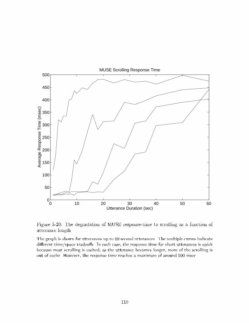
0 10 20 30 40 50 600
50
100
150
200
250
300
350
400
450
500
Utterance Duration (sec)
Ave
rage
Res
pons
e T
ime
(mse
c)
MUSE Scrolling Response Time
Figure 5-20: The degradation of MUSE response-time to scrolling as a function ofutterance length.
The graph is shown for utterances up to 60 second utterances. The multiple curves indicate
di�erent time/space tradeo�s. In each case, the response time for short utterances is quick
because most scrolling is cached; as the utterance becomes longer, more of the scrolling is
out of cache. However, the response time reaches a maximum of around 500 msec.
110

0 10 20 30 40 50 6020
40
60
80
100
120
140
Utterance Duration (sec)
Ave
rage
Res
pons
e T
ime
(mse
c)
SAPPHIRE Response Time to Scrolling
Figure 5-21: The correlation between Sapphire's response time to scrolling and ut-terance duration.
The response time for utterances less than about 45 seconds grows linearly with utterance
duration, but remains very fast. Beyond 45 second utterances, Sapphire was beginning to
page to disk because it was using more memory than was available; this causes the response
time to increase sharply.
111

8 10 12 14 16 18 20 220
50
100
150
200
250
300
350
400
450
500
Memory Used (MB)
Res
pons
e T
ime
(mse
c)
MUSE Response Time vs Memory Usage
Figure 5-22: The tradeo� of average response time for scrolling versus memory usage,
for the MUSE speech analysis tool.
A �xed duration utterance (20 seconds) was loaded into the tool, and the cache parameters
were varied to achieve di�erent points in the graph.
112

user behavior, multi-processor computers, local and remote on-disk storage, video-
card performance, how many displays, resolution and color depth of the displays,
fast networking to other computers, etc. Neither MUSE nor Sapphire are adaptive
across these run-time variations. For example, neither is able to make use of a dual-
processor computer, despite the abundance of such computers now. Also, neither will
appreciably alter its run-time strategy when running on a slower or faster computer.
5.3 Summary
This chapter has evaluated the MUSE architecture and implementation along two
fronts. First, �ve example MUSE tools were described, demonstrating novel forms
of interactivity made possible by MUSE's design. Each tool provides a continuous
interface to the user, allowing the user to change many aspects of the computation,
and receive a rapid corresponding response. Furthermore, MUSE compares favorably
with Sapphire on several of the proposed metrics for interactivity. The next chapter
discusses some programmatic issues of MUSE, while Chapter 7 analyzes the results
from this chapter, discusses issues and future work, and concludes the thesis.
113

Chapter 6
Programming MUSE
This chapter delves into some of the programmatic aspects of MUSE. In particu-
lar, I describe the steps needed to design and create a MUSE tool, illustrating the
process by describing the full source code for the spectral slice tool, as well as the
steps needed when extending MUSE with new functionality. For ease of reference,
I distinguish three classes of individuals who might work with MUSE. The system
programmer is someone who extends the MUSE toolkit by creating new built-in func-
tions; the system programmer must get \under the hood," really understanding the
internal implementation of MUSE in order to augment it with new functionality. The
programmer is someone who uses MUSE to construct a new tool: he or she writes
a complete MUSE program, in Python, making use of the existing built-in functions
and datatypes. Finally, the user interacts with existing MUSE tools. This chapter
describes the steps which need to be taken when creating MUSE tools (the program-
mer) and when extending MUSE (the system programmer); the user's viewpoint was
summarized in the last chapter.
6.1 The Programmer
The programmer creates an interactive tool by writing a complete Python program
that calls on both MUSE and Python to compute di�erent aspects of the tool. The
tight integration between MUSE and Python gives the programmer the freedom to
114

execute some computation in MUSE and some in Python, as appropriate. In this
section I describe the organization of a typical MUSE tool, by analyzing the source
code for the spectral slice tool, described in Chapters 1 and 5.
When building a new tool, the programmer must divide the necessary functional-
ity between MUSE and Python. Certain computations are best done in MUSE. For
example, loading a waveform and computing spectral representations should be done
within MUSE so as to hide di�cult computational details such as when which por-
tions of the waveform are actually loaded, when to compute spectral representations
and when to recompute which images in response to the user's actions. In addition,
variables which will need to change frequently, and whose changes will impact many
other variables, should be represented in MUSE instead of Python in order to take
advantage of the fact that MUSE manages such changes automatically. Naturally,
when expressing the computations in MUSE, the programmer must decompose the
necessary functionality according to MUSE's declarative, functional design. For ex-
ample, the process of scrolling might be thought of as a highly imperative series of
steps copying images around, but in MUSE, should be thought of as merely changing
the view-variable of the window displaying the image.
6.1.1 Tk
Other aspects of a tool should be implemented in Python, such as using Python's
interface to Tcl's Tk, Tkinter, to design the layout of the tool's interface and create
the callback functions to respond to the user's actions. Tk models user interactivity
by providing common widgets, such as Scrollbars, Buttons and Scales, which may
be created and \packed" into certain places in the tool. At run-time, when the
user directly manipulates one of these widgets, a corresponding callback function, in
Python, is called. This function must take whatever actions are necessary to re ect
the change initiated by the user. In MUSE tools, the callback functions typically
initiate a change in a MUSE variable, and then return. That change may impact
many other MUSE variables, usually including one of the images being displayed to
the user.
115

In order to directly integrate MUSE and Tk, there is one function, muse window,
which is a MUSE function that returns a proper Tk widget: it can be sized to a
speci�ed width and height, \packed" into other Tk widgets, and respond to standard
X events using Tk's bind command. The programmer uses this function to display
MUSE images to the user. The function takes integer MUSE arguments corresponding
to the scroll view of the image; in order to subsequently scroll, these MUSE variables
are changed. For example, the action taken by the Python callback function of a
scrollbar should be to change such the view variable of the corresponding windows,
subject to the extent of allowable scrolling. Making the view variables standard
MUSE integers isolates how the user scrolls (e.g., with a Scrollbar, or by clicking and
dragging) from how MUSE implements scrolling, thereby allowing exibility in the
resulting interface.
6.1.2 Memory Management
All objects in MUSE are allocated according to Python's memory model, which uses
reference counting to measure how many pending references there are to an object.
When the count reaches zero, Python frees the object, thereby reclaiming the memory.
This automated memory management, in contrast to a language such as C, greatly
simpli�es the programmer's e�orts. However, the system programmer, when extend-
ing MUSE by adding functionality implemented in C, must understand Python's
model so as to conform to it.
6.1.3 Spectral Slice Tool
The best way to understand how to build MUSE tools is to study an example; in this
section I describe all of the source code for the spectral slice tool. The source code
is rather lengthy (328 lines) as it includes numerous details for the tool's interface,
MUSE computations, and interface logic. The code is roughly divided into four sec-
tions, one for each window in the tool. In this tool, MUSE handles the computation
of the images for the top three windows, while the bottom window consists entirely
116
of Tk widgets (Scrollbars, Labels, Scales and RadioButtons). The source code corre-
sponding to each window will be described. A snapshot of the running tool is shown
in Figure 6-1; for reference, the complete numbered source code (328 lines) is shown
in Figures 6-2 through 6-8.
6.1.4 Waveform Window
The waveform window, shown in the center of Figure 6-1, displays four separate
images. The top is a zoomed-in waveform image with two image overlays: the time
mark (which tracks the user's mouse) and the analysis window. The next two are the
phonetic and orthographic transcriptions, while the �nal is a time axis. The MUSE
code producing these images begins on line 31. The waveform image is constructed
functionally, by producing the three images (wav v, mks v and win v) and calling the
v overlay function (line 68). In MUSE, an image is only de�ned for a certain subset
of pixels, which will vary from one image to another and as the image undergoes any
changes. Therefore, for some images, it is necessary to overlay them onto a blank
background image, which is what bg (created on line 27) is. Further, images may
have arbitrary widths and heights; the image produced by the v blank function is
e�ectively in�nite in expanse. Therefore, the same background image is used across
all three MUSE windows.
The muse window function is a Tk widget which can be packed just like all other
Tk widgets; this is how MUSE interfaces with Tk. The tool calls muse window eight
times, once for each image which needs to be independently laid out according to Tk's
geometry manager. The function takes a number of arguments, including a parent Tk
object in which the widget is packed, a requested width and height, the MUSE image
to display, and an xview and yview which control scrolling of the image. The integer
variable xv, de�ned on line 21, controls the current view, and changes whenever the
user scrolls. It is initialized to 15000.
The variable wav v is the waveform image drawn to a certain time-scale and
is created by calling the v waveform function on line 57. That function takes a
waveform, wav, a foreground color, the time-scale (tsc) and the yscale (ysc). The
117

Figure 6-1: An interactive FFT, LPC and Cepstrum spectral slice tool.
The user sees three overlaid spectral slices, computed at a variable point in the displayed
waveform: the standard FFT, an LPC spectrum, and a cepstrally smoothed spectrum.
Many parameters in the computation may be changed, with a continuous corresponding
response. The user is able to compare and evaluate many issues related to signal represen-
tation for speech recognition.
118

1 import _allmm, os, signal, bscroll, string
import Tkinter, types, wls
tk = Tkinter
5 from muse import *
from muse_fcn import *
os.chdir('/usr/users/mike/twav/') # Input files
wav_file = mvalue('si1212-b-mgar0.wav')
10 wrd_file = mvalue('si1212-b-mgar0.wrd')
phn_file = mvalue('si1212-b-mgar0.phn')
wav = nist_wav(wav_file) # Load the files
trans = o_transcription(phn_file)
15 trans_wrd = o_transcription(wrd_file)
srate = wav.force().srate # Compute wav duration
nums = wav.force().nums
wav_dur = m_div(m_float(nums), srate)
20
xv = mvalue(15000) # X-view (scrolling)
tsc = mvalue(10000.0) # Time-scale (zoom)
wd = mvalue(700) # Width of the waveform,
# transcription, axis windows
25 tm = mvalue(1.525) # The time-mark value
# (starts at 1.525 seconds)
bg = v_blank('#d9d9d9') # A blank background image
30
# WAVEFORM WINDOW
root = tk.Tk() # Tk stuff
InitMuseTk(root)
35 root.title('MUSE: Waveform')
root.geometry('701x262+151+243')
ax_f = tk.Frame(root, relief='sunken', bd=1)
ax_f.pack()
40 win_dur_ms = mvalue(5.0) # Analysis window
win_dur = m_mul(win_dur_ms, 0.001)
num_point = m_int(m_mul(win_dur, srate))
win = mvalue(o_hanning(num_point))
win_v = v_vector(win, # Analysis window image
45 width=m_int(m_mul(tsc, win_dur)),
height=65,
ymax=0.0, yrange=1.0, fg='red', lw=2,
auto=1,
xctr=m_int(m_mul(tsc, tm)),
Figure 6-2: Source code (lines 1{49) for spectral slice tool.
119

50 fast=1, yoffset=-65)
mks = o_var_marks(tm) # Create time-marks & image
mks_v = v_marks(mks, tsc)
55
ysc = mvalue(0.01) # Scale for waveform-view
wav_v = v_waveform(wav, 'darkblue', tsc, ysc) # Waveform image
trans_v = v_graph(trans, tsc, # Transcription image
60 height=40,
show_boundaries=0)
trans_wrd_v = v_graph(trans_wrd, tsc, # Word transcription image
height=40,
65 show_boundaries=0)
wav_w = muse_window(ax_f, width=wd, height=140, # Window to display waveform,
image=v_overlay(bg, wav_v, # time mark, analysis window
mks_v,
70 win_v),
xview=xv, yview=-70)
wav_w.force().pack()
def motion(ev): # Respond to motion events
75 tm0 = (xv.force()+ev.x)/tsc.force()
tm.change(tm0)
wav_w.force().bind('<Motion>', motion)
wav_w.force().bind('<Enter>', motion)
80 # Window for trans
w_trans = muse_window(ax_f, width=wd, height=40,
image=v_overlay(bg, trans_v),
xview=xv, yview=-60)
w_trans.force().pack()
85
# Window for word trans
w_trans_wrd = muse_window(ax_f, width=wd,
height=40,
image=v_overlay(bg,
90 trans_wrd_v),
xview=xv, yview=-60)
w_trans_wrd.force().pack()
tax_v = v_axis(tsc) # Horizontal time axis image
95 tax_w = muse_window(ax_f, width=wd, height=20, # Window to display axis
image=v_overlay(bg, tax_v),
xview=xv)
tax_w.force().pack()
Figure 6-3: Source code (lines 50{99) for spectral slice tool.
120
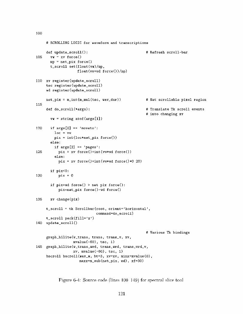
100
# SCROLLING LOGIC for waveform and transcriptions
def update_scroll(): # Refresh scroll-bar
105 vw = xv.force()
np = net_pix.force()
t_scroll.set(float(vw)/np,
float(vw+wd.force())/np)
110 xv.register(update_scroll)
tsc.register(update_scroll)
wd.register(update_scroll)
net_pix = m_int(m_mul(tsc, wav_dur)) # Net scrollable pixel region
115
def do_scroll(*args): # Translate Tk scroll events
# into changing xv
vw = string.atof(args[1])
120 if args[0] == 'moveto':
loc = vw
pix = int(loc*net_pix.force())
else:
if args[2] == 'pages':
125 pix = xv.force()+int(vw*wd.force())
else:
pix = xv.force()+int(vw*wd.force()*0.20)
if pix<0:
130 pix = 0
if pix+wd.force() > net_pix.force():
pix=net_pix.force()-wd.force()
135 xv.change(pix)
t_scroll = tk.Scrollbar(root, orient='horizontal',
command=do_scroll)
t_scroll.pack(fill='x')
140 update_scroll()
# Various Tk bindings.
graph_hilite(w_trans, trans, trans_v, xv,
mvalue(-60), tsc, 1)
145 graph_hilite(w_trans_wrd, trans_wrd, trans_wrd_v,
xv, mvalue(-60), tsc, 1)
bscroll.bscroll(wav_w, bt=3, xv=xv, minx=mvalue(0),
maxx=m_sub(net_pix, wd), xf=30)
Figure 6-4: Source code (lines 100{149) for spectral slice tool.
121

150
# SPECTRAL SLICES WINDOW
slc_t = tk.Toplevel() # Tk stuff
slc_t.geometry('374x195+151+10')
155 slc_t.title('MUSE: Spectral Slice')
slc_f = tk.Frame(slc_t, relief='sunken', bd=1)
slc_f.pack(fill='both', expand='yes')
slc_ax_f = tk.Frame(slc_f)
slc_ax_f.pack(side='left', fill='y')
160
slc_wd = mvalue(350) # Width/height of slices
slc_ht = mvalue(150)
lpc_order = mvalue(16) # LPC order
165
win_wav = o_window_wav1(wav, win, tm) # Windowed waveform
fft = o_fft(win_wav, 128) # Standard FFT
170 lpc = o_fft(o_lpc(win_wav, lpc_order), 64, 1) # LPC spectrum & peaks
lpc_peaks = o_peaks(lpc)
cepstral_order = mvalue(10) # Cepstral order
175 cep = o_cepstrum_smooth(fft, # Cepstral-smoothed spectrum
cepstral_order,
128)
mx1 = o_max_vector(fft) # Max value of all slices
180 mx2 = o_max_vector(lpc)
mx3 = o_max_vector(cep)
vec_max = mvalue(o_max(mx1, mx2, mx3))
ymax = m_add(10.0, vec_max)
185 yrange = mvalue(80.0) # Spectral-slice images
v_cep = v_vector(cep, width=slc_wd,
height=slc_ht,
ymax=ymax, yrange=yrange,
fg='red', lw=2)
190 v_fft = v_vector(fft, width=slc_wd,
height=slc_ht,
ymax=ymax, yrange=yrange,
fg='black', lw=2)
v_lpc = v_vector(lpc, width=slc_wd,
195 height=slc_ht,
ymax=ymax, yrange=yrange,
fg='blue', lw=2,
peaks=lpc_peaks)
Figure 6-5: Source code (lines 150{199) for spectral slice tool.
122

200 slc_img = mvalue(v_overlay(bg, v_fft, # Overlaid slice images
v_lpc, v_cep))
slc_ysc = m_div(m_mul(-1.0, slc_ht), yrange) # Vertical db axis, adapting
v_ax = v_axis(slc_ysc, orient='vertical', # to max vector
205 min_pix_inc=30, digits=0)
slc_yv = m_mul(ymax, slc_ysc)
ax_w = muse_window(slc_ax_f,
width=23, height=slc_ht,
image=v_overlay(bg, v_ax),
210 yview=slc_yv, xview=-2)
ax_w.force().pack(side='top')
fsc = 2000.0*slc_wd.force()/srate.force()
fax_v = v_axis(fsc, # Horizontal frequency axis
215 min_pix_inc=25)
fax_w = muse_window(slc_f, width=slc_wd,
height=20, yview=5,
image=v_overlay(bg, fax_v))
fax_w.force().pack(side='bottom')
220
xc = mvalue(0) # Slices window & cursors
yc = mvalue(0)
slc_w = muse_window(slc_f,
width=slc_wd, height=slc_ht,
225 image=slc_img,
xcursor=xc, ycursor=yc)
xc.change(slc_w.force().xpos)
yc.change(slc_w.force().ypos)
slc_w.force().pack(fill='both', expand='yes')
230
# CheckButtons allowing user to choose which slices are overlaid
def cf_change():
235 a = c1.get()
b = c2.get()
c = c3.get()
if not a and not b and not c:
240 slc_img.change(bg)
elif not a and b and not c:
slc_img.change(v_overlay(bg, v_lpc))
vec_max.change(mx2)
elif a and not b and not c:
245 slc_img.change(v_overlay(bg, v_fft))
vec_max.change(mx1)
elif a and b and not c:
slc_img.change(v_overlay(bg, v_fft, v_lpc))
vec_max.change(o_max(mx1, mx2))
Figure 6-6: Source code (lines 200{249) for spectral slice tool.
123

250 elif not a and not b and c:
slc_img.change(v_overlay(bg, v_cep))
vec_max.change(mx3)
elif not a and b and c:
slc_img.change(v_overlay(bg, v_lpc, v_cep))
255 vec_max.change(o_max(mx2, mx3))
elif a and not b and c:
slc_img.change(v_overlay(bg, v_fft, v_cep))
vec_max.change(o_max(mx1, mx3))
else:
260 slc_img.change(v_overlay(bg, v_fft, v_lpc, v_cep))
vec_max.change(o_max(mx1, mx2, mx3))
c1 = tk.IntVar()
c2 = tk.IntVar()
265 c3 = tk.IntVar()
slc_cf = tk.Frame(slc_t, relief='sunken', bd=1)
slc_cf.pack(fill='x')
270 cf1 = tk.Checkbutton(slc_cf, text='FFT', fg='black',
command=cf_change, variable=c1)
cf2 = tk.Checkbutton(slc_cf, text='LPC', fg='blue',
activeforeground='blue',
command=cf_change, variable=c2)
275 cf3 = tk.Checkbutton(slc_cf, text='Cepstrum', fg='red',
activeforeground='red',
command=cf_change, variable=c3)
tk.Label(slc_cf, text='Overlay: ').pack(side='left')
cf1.pack(side='left')
280 cf2.pack(side='left')
cf3.pack(side='left')
cf1.select()
cf2.select()
285 cf3.select()
Figure 6-7: Source code (lines 250{285) for spectral slice tool.
124

290 # WINDOWED WAVEFORM WINDOW
wwav_t = tk.Toplevel() # Tk stuff
wwav_t.title('MUSE: Windowed Waveform')
wwav_t.geometry('307x195+546+10')
295 wwav_f = tk.Frame(wwav_t, bd=1, relief='sunken')
wwav_f.pack()
wv5_max = o_max(o_max_vector(win_wav), # To normalize
m_mul(-1.0,
300 o_min_vector(win_wav)))
wwav_v = v_vector(win_wav, # Windowed waveform image
width=304, height=190,
ymax=wv5_max,
305 yrange = m_mul(wv5_max, 2.2),
lw=2)
wwav_w = muse_window(wwav_f, width=304,
height=190, yview=-10,
image=v_overlay(bg, wwav_v))
310 wwav_w.force().pack()
# CONTROL WINDOW
ctl = tk.Toplevel(width=500) # Tk stuff
315 ctl.title('MUSE: Control')
ctl.geometry('701x143+151+543')
wls._slider(ctl, win_dur_ms, min=2.0, max=50.0,
name='Win Dur', label='ms',
320 fmt='%.1f').pack(fill='x')
wls._slider(ctl, lpc_order, min=1, max=50,
name='LPC Order').pack(fill='x')
wls._slider(ctl, cepstral_order, min=1, max=128,
name='Cepstral Order').pack(fill='x')
325 wls._slider(ctl, ysc, min=0.001, max=0.5,
name='Yscale', fmt='%.1f',
factor=1000.0).pack(fill='x')
wls._tscale(ctl, tsc).pack(fill='x')
wls._win_choice(ctl, win, num_point).pack(fill='x')
330
muse_mainloop(0, 0)
Figure 6-8: Source code (lines 286{332) for spectral slice tool.
125
waveform in turn was created on line 13 by calling the nist wav function which loads
a NIST standard waveform given a string �lename.
The variable mks v is created with the v marks function on line 54. In general,
v marks produces an image for an arbitrary collection of marks. However, for this
tool, the marks variable, mks, consists of a single time mark, created on line 53
with the o var marks function. That function is unusual in MUSE because it will
propagate changes in two directions: if the mks variable is ever changed, the oating
point input to the function, tm, will be changed, and vice-versa. tm is a oating point
number corresponding to the analysis time, and is created on line 25.
The third overlaid image, win v, is created on line 44 with the v vector function.
There are numerous inputs provided to the function, to ensure that the scale is correct
and that the displayed vector is always centered on the displayed time-mark. The �rst
input to the function is win, which is the analysis window, as computed on line 43, by
applying the o hanning function. Note that the output of o hanning is \wrapped"
within a new MUSE variable; this illustrates the important point that the mvalue
function input may actually be another MUSE value. This is used in this case because
the tool will need to replace the value of win with an entirely new window when the
user changes the analysis window.
The input to o hanning is the number of points in the window, computed by
multiplying the window duration by the sample rate, and casting the result to an
integer. These computations are done using the basic MUSE functions m mul and
m int, but also could have been done directly in Python. However, because the
window duration may change in the future (when the user slides the corresponding
scale), or the waveform's sample rate may change, by doing the computations in
MUSE instead of Python, the programmer does not need to worry about such future
changes as they will be propagated automatically.
The result of overlaying these four images is the image which is actually seen by
the user in the middle waveform window. Many aspects of the computations leading
to this image may change: the analysis time may change, the duration and type of
window, the time scale or the waveform's yscale. The programmer does not have to
126

deal with such changes; instead, in response to each change, MUSE will propagate
the change and subsequently recompute the necessary images.
Lines 74|78 show the Python functions which cause the tm variable to be changed
whenever the user moves the mouse over the waveform window. Tk's bind functions
causes any Motion or Enter events to call the Python motion function, which in turn
will translate the x pixel of the motion into a time, using the tsc and xv variables.
Note the use of the force methods of these variables, which translate the current
value of a MUSE variable into Python. As a consequence of the call to tm.change on
line 76, much computation will take place; this is all hidden from the programmer.
The two transcription images are created using the v graph function applied (on
lines 59 and 63) to the phonetic and orthographic transcription graphs, trans and
trans wrd. The v graph function turns a graph into the corresponding image, ac-
cording to a time-scale and other parameters. The trans and trans wrd variables
are created on lines 14 and 15, loaded from �les. Each of the transcription images
is overlaid onto the blank background and then placed in its own muse window and
then packed under Tk's geometry model (lines 81|91).
Finally, the axis image, tax v, is created on line 93 using the v axis function. The
v axis function creates an axis image either horizontally (the default) or vertically,
according to a speci�ed scale. In this case the time-scale tsc is provided. The time
axis also has its own window, on lines 94|97. The same xview, xv, is provided to
each of these windows to ensure that when the user scrolls, all images scroll together.
Lines 100|140 provide the logic for managing both scrolling and highlighting
edges in the transcription whenever the user moves the mouse over them. Manag-
ing the scrollbar requires two directions. First, whenever the view variable, xv, or
the window width, wd, or the scrollable image size, represented by net pix change,
the scrollbar must be redrawn accordingly. Lines 107|109 illustrate the register
method, available for all MUSE variables, which will call a Python function, in this
case update scroll, whenever their value changes. In response to such changes, the
scrollbar is redrawn. The other direction is to respond to the user's actions when he
or she grabs the scrollbar; when the scrollbar is created and packed (lines 129{131),
127
the Python function do scroll, de�ned on lines 113{127, is provided. This function,
which is called whenever scrolling actions are taken by the programmer, is fairly com-
plex in order to handle the multiple ways in which the user may scroll. Each of the
cases involves computing a new value for xv, clipping it according to a minimum and
maximum, and then changing the value of xv (line 127). All of the images in the
waveform window will be changed when that line is executed.
6.1.5 Spectral Slices Window
The MUSE code for the spectral slices window, shown in the upper left of Figure 6-1,
starts on line 143. Lines 145|149 create a new toplevel window and frame in which
to pack the spectral slice window. Three spectral slice images are overlaid, all with a
width and height speci�ed by slc wd and slc ht de�ned on lines 153 and 154. The
v fft image, created on line 181, corresponds to the standard FFT, computed with
the o fft function on line 160. The input to that function is win wav, created with
the o window wav1 function on line 158; this function applies the provided analysis
window win to the provided waveform wav at the speci�ed time tm, resulting in
the vector variable fft. Similarly, v lpc and v cep are created, by applying an
LPC spectra function and a cepstral smoothing function. Note that all three of
the v vector calls provide ymax as the maximum level to draw; this is a variable
computed on line 183 which is always 10.0 plus the maximum of all vectors. In this
fashion, the spectral slice window, and corresponding vertical axis, will constantly
renormalize itself to the maximum of all vectors. The three images are overlaid over
the background on line 189; the extra mvalue call allows the image to be changed,
which will happen when the user clicks on the buttons to change which slices are
overlaid (the code on lines 232|285 handles this). In addition to the spectral-slice
window, there are two axes, created on lines 204|219. The yview provided to the
vertical axis window on line 210 is computed from the ymax variable, so that the
axis will also be e�ectively scrolled to adapt to the maximum of the vectors being
displayed.
Finally, the muse window which displays the spectral slices is on line 223. Note
128

how the cursors are created. The x and y cursors for that window are actually integer
valued variables; by creating two muse variables, xc and yc �rst, and then binding
their values to be the xpos and ypos of the window, the cursors will perpetually
follow the users mouse when in that window.
6.1.6 Windowed Waveform Window
The windowed waveform window displays the vector corresponding to the windowed
waveform fragment in the upper right window of Figure 6-1; the corresponding MUSE
code is on lines 290|310. The windowed waveform, win wav, was already computed
on line 166; all that is necessary to display it is to create a Tk toplevel window and
frame. In order to normalize the display, the maximum of the windowed waveform
is computed on line 298, and then used to set the yscale of the v vector call on line
302.
6.1.7 Control Window
The control window is the bottom window in Figure 6-1, and contains many sliders to
change various parameters. Each of these sliders is created using the slider object,
de�ned in a separate �le. This class essentially creates a Tk slider and corresponding
label, packs them together, and then responds to the user's actions by changing the
corresponding MUSE variable. For example, the call on line 318 de�nes the slider
which controls the analysis window duration in ms. The MUSE variable win dur ms,
originally created on line 40, will change whenever the user slides the slider. Finally,
the call to muse mainloop on line 331 allows MUSE to take control of actually running
the tool.
6.1.8 Summary
The spectral slices tool is a fairly involved MUSE tool and illustrates some impor-
tant aspects of creating tools in MUSE. MUSE is used for the internal, back-end
computations of a tool, while Python is used to manage the Tk interface (packing
129

and layout as well as responding to the user's actions). As can be seen with the
tool, MUSE tools make heavy use of simple types for MUSE variables, for example
the integer valued xv, oating point valued wav dur, etc. Further, these variables
are used in many places (e.g., xv appears 14 times in the source code). For these
variables, the computation is expressed in MUSE and not Python not because of the
expected compute intensive nature, but rather so that MUSE can automatically han-
dle change propagation and response. The vertical axis of the spectral-slices window
automatically adapts according to the maximum of all of the vectors; such adapta-
tion would be a nuisance for the programmer to express in Python, but expressed in
MUSE, once, is quite straightforward. Most importantly, MUSE hides the di�culty
of managing changes to a variable: throughout the program, the values MUSE vari-
ables are changed without regard as to the eventual impact. Finally, lines 43 and
200 illustrates the useful application of the mvalue function to \wrap" a value which
already a MUSE variable, thereby allowing it to be changed in the future.
Also illustrated is the tight integration of MUSE with Python. The value of a
MUSE variable can be extracted into Python with the force method, illustrated on
lines 75, 105, 106, 107, 122, etc. The reverse is achieved by calling mvalue, which
is used all over the program to create new MUSE variables. Finally, when the value
of a MUSE variable is changed, a Python function can be called using the register
method, as illustrated on lines 110|112. The Python function may do other things,
including initiating changes in other variables.
6.2 System Programmer
The system programmer is someone who might extend MUSE with additional func-
tionality. Depending on the nature of the additional functionality, this process can
range from straightforward to di�cult. MUSE's design certainly introduces addi-
tional complexities in the process of implementing new functionality, at the tradeo�
of o�ering a simple and high-performance interface to MUSE programmers. Having
to provide a lazy evaluation interface for large datatypes, as well as responding to
130

incremental computation, can greatly increase the complexity of implementing a new
function.
MUSE can be extended in two di�erent ways. First, a whole new datatype can
be created. This is a fairly involved process as it requires understanding the needs
and potential applications of the datatype well enough to design the functional, lazy
evaluation representation for the datatype as well as the allowed incremental changes
for the datatype. Second, a new built-in function, using existing datatypes, could be
added. This is typically more straightforward, but due to some aspects of MUSE's
design (lazy evaluation and incremental computation), the process can become com-
plex.
6.2.1 New Datatypes
When adding a new datatype to MUSE, the system programmer must think carefully
about which datatypes to add, how the datatype should be represented, functionally,
as well as how the datatype may incrementally change. This design process is typi-
cally very iterative, and like all design processes, involves tradeo�s. One design issue
is the extent of granularity : should there be many small and simple datatypes and
corresponding built-in functions, or fewer larger ones? On the one hand, datatypes
should be selected so as to expose many of the intermediate steps of complex calcu-
lations. By doing so, MUSE is able to work with the intermediate variables, allowing
for the application of incremental change and exible caching. But on the other hand,
by making the datatypes too �ne, e�ciency is sacri�ced and tools using the datatypes
will lose interactivity. A further need which must be taken into account during design
is what sorts of tools and functionality will need to be created based on the datatypes.
As an example, consider the process of extending MUSE to include a new datatype
representing a hierarchical clustering of a collection of vectors. Such a datatype might
index the vectors with integers, maintain parent/child relationships between them and
record the distances between merged clusters. This datatype could be the output of
a bottom-up or top-down clustering algorithm which takes as input any of a variety
of distance metrics, or could be used to represent a dendrogram segmentation [12].
131

Tools using such a datatype might allow the user to vary the distance metric and other
parameters of the clustering function in order to interactively observe the resulting
impact.
The appropriate functional representation should be chosen so as to allow e�cient
computation of portions of the datatype. For example, when clustering very large
collections of vectors, we may only be interested in which clusters particular collections
of vectors belong to. A functional interface might therefore allow looking up the
integer indices of all vectors, and looking up a cluster identity for an individual vector.
In this fashion, functions which compute a clustering would be able to compute, on-
demand, only those portions of the clustering which were needed.
The datatype must also be designed to support incremental computation. Perhaps
a clustering would be designed to allow the addition, deletion or replacement of a
single vector. This would allow tool users to explore the incremental impact as the
dataset is changed slightly. In addition, the datatype could incrementally change
by leaving the vectors to the same but having some of the distances between them
change. This might occur when the distance metric of a particular clustering function
is changed, but the universe of vectors remains the same.
In addition to adding entirely new datatypes, MUSE can also be extended by
augmenting an existing datatype to include new kinds of incremental change. One
candidate might be the waveform, which currently supports no incremental change.
For example, one could imagine a powerful concatenative speech synthesis tool al-
lowing the user to explore alternatives for concatenative synthesis. A word sequence
could be typed in, at which point the tool synthesizes a possible utterance. The ut-
terance could then be edited, by stretching or shrinking the duration of a segment,
or changing the energy or pitch of a segment. After each change, the user could
play the utterance to hear the e�ect. Alternatively, the metrics used to search for
the ideal segment sequence could be changed so as to hear the impact. In order to
support such a tool, the waveform datatype might be extended in order to allow
splicing of an arbitrary range of samples with new samples. Of course, all functions
which may be applied to waveforms would need to be correspondingly updated in
132

order to accommodate such incremental changes. The v waveform function would
need to translate such a change into an incremental change in its output image, while
the o window wav function (used to compute the STFT) would need to propagate the
change to an incremental change on its output frames, for example. As is illustrated
by this process, the design of the datatype re ects the expected usage of tools based
on the datatype.
6.2.2 New Functions
There are several issues that impact the process of adding a new function to MUSE.
The system programmer is able to make use of existing functions and datatypes, which
can greatly simplify the function when compared to the corresponding e�ort to extend
Sapphire. However, built-in functions in MUSE must support a lazy-evaluation inter-
face according to their output datatype, as well as manage any incremental changes
on their inputs.
For example, consider adding the necessary functionality to enable tools to draw
a graphical representation of the hierarchical cluster datatype, called a dendrogram1.
An example of such a dendrogram, derived from the bigram distribution of words
from ATIS [31], instead of acoustic vectors, is shown in Figure 6-9. Because images
are treated as �rst-class datatypes, and the process of drawing an image on the screen
involves several independent functions, adding this functionality to MUSE is fairly
focused to implementing only the novel functionality itself. The programmer needs
to create a new Python class which will be instantiated whenever the new function is
applied. Like the o fft example from Section 4.3.2, this class must de�ne an init
method to create the return variable and declare dependencies on inputs. Unlike
o fft, because this function produces an image, which is a non-atomic datatype,
instead of a vector, the function would provide a draw method which is able to draw
a requested rectangular region of the image. According to the rectangular region, and
according to how the hierarchical datatype is represented, the draw function would
1For example, something like the dendrograms drawn by Splus.
133

A
A_M
AF
TE
RN
OO
N
AIR
CR
AF
TA
IRP
LAN
E
AM
ER
ICA
N
AN
AN
Y
AT
LAN
TA
AU
GU
ST A
VA
ILA
BLE
BA
LTIM
OR
E
BE
BO
OK
BO
ST
ON
CH
EA
PE
ST
CIT
Y
CLA
SS
CO
AC
H
CO
NT
INE
NT
AL
CO
ST
DA
LLA
S
DA
LLA
S_F
OR
T_W
OR
TH
DA
Y
DE
LTA
DE
NV
ER
DO
LLA
RS
DO
WN
TO
WN
EA
RLI
ES
T
EA
ST
ER
N
EC
ON
OM
Y
EIG
HT
EIG
HT
Y
EV
EN
ING
FA
RE
FA
RE
S
FIF
TE
EN
FIF
TY
FIN
D
FIR
ST
_CLA
SS
FIV
EFLY
FO
RT
Y
FO
UR
FR
IDA
Y
GE
T
GIV
E
GO
GR
OU
ND
HU
ND
RE
D
INF
OR
MA
TIO
N
IT
JULY
KIN
D
KN
OW
LAT
ES
TLEA
ST
LOW
ES
T
MA
KE
MA
Y
ME
AL
ME
ALS
MO
ND
AY
MO
RN
ING
MO
ST
NE
ED
NIN
E
NIN
ET
Y
NO
NS
TO
P
NO
VE
MB
ER
O+
CLO
CK
OA
KLA
ND
OH
ON
E
ON
E_W
AY
P_M
PH
ILA
DE
LPH
IA
PIT
TS
BU
RG
H
PLA
NE
RE
TU
RN
RO
UN
D_T
RIP
SA
N_F
RA
NC
ISC
O
SA
TU
RD
AY
SC
EN
AR
IO
SE
RV
ED
SE
RV
ICE
SE
VE
N
SE
VE
NT
Y
SIX
SIX
TY
ST
OP
OV
ER
SU
ND
AY
TA
KE
TE
LL
TH
ER
E
TH
ES
E
TH
IRT
Y
TH
IS
TH
OS
E
TH
RE
E
TH
UR
SD
AY
TIC
KE
T
TIM
E
TIM
ES
TR
AN
SP
OR
TA
TIO
N
TR
AV
EL
TU
ES
DA
Y
TW
EN
TY
TW
O
TY
PE U
_S_A
IR
UN
ITE
D
US
ED
WA
NT
WA
SH
ING
TO
N
WE
DN
ES
DA
Y
WIL
LW
OU
LD
ZE
RO
NIL
02
46
Figure 6-9: An example dendrogram.
then force the necessary portion of the input clustering, and then actually draw the
image. Note that the function is only responsible for actually drawing itself, and does
not have to manage caching the image, scrolling the image, managing overlays such as
time marks and cursors, displaying the image, nor dealing with window events such
as Expose and Configure.
The new function must respond to incremental changes in the clustering. De-
pending on how the cluster datatype was designed, this process may be complex. For
example, if a new vector is added, it may be necessary to redraw the entire bottom
portion of the image to \make space" for the new vector at the bottom of the image.
The function is noti�ed of changes to its input because it registered for such changes
in its init method; when such changes occur, the function which it provided dur-
ing registration will be called. This function in turn, would compute a rectangular
bounding box outlining the change in its output image, and then proceed to notify its
output of this change. The function need not worry about subsequent recomputation
of the a�ected portion; this occurs through the normal channels of lazy evaluation.
134
The above description contains the necessary steps when adding a fully capable
built-in function to MUSE. However, certain shortcuts may be taken. For example,
a simple way to propagate incremental changes would be to always declare that the
entire output image must be redrawn in response to any change. This sacri�ces run-
time e�ciency, but makes it easier to add such functions. Depending on the typical
compute-time of the function, this tradeo� may or may not be worthwhile.
Also, depending on the nature of the necessary computations, it may be worth-
while implementing part of the function in C. Fortunately, Python makes this process
rather straightforward; the system programmer is able to create a new Python module
containing any number of functions. Typically, within the compute or draw method
of the new MUSE function's class, the function will then call the C function to carry
out compute-intensive portions of its computation. The one substantial complexity
which arises when writing the C code is conforming to Python's reference counting
memory management model; di�cult bugs arise when one forgets to increment the
reference count to a Python object. However, once this is done correctly, Python's
e�ective memory management model naturally extends to the new MUSE function.
6.2.3 Summary
In summary, the process of extending MUSE with new functionality can be fairly
complex and entails di�erent issues from extending existing systems like Sapphire.
The needs of particular tools must be understood and translated into a design for new
datatypes and functions, or new forms of incremental change for existing datatypes.
Then, the changes need to be implemented according to MUSE's computation model,
including lazy evaluation and incremental change. Depending on the nature of the
new functionality, translating known algorithms so that they support incremental
computation can be fairly di�cult. Finally, the code implementing the new function
or datatype is actually written as either all Python code, or a combination of Python
and C.
135

Chapter 7
Conclusions
This chapter analyzes the results of the evaluation, draws a detailed comparison
between MUSE and Sapphire, discusses some of the interesting issues that surfaced
while creating MUSE, suggests directions for future work, and concludes the thesis.
I conclude that the MUSE architecture successfully enables �nely interactive speech
tools. These tools would make an excellent aid in an educational setting. However,
MUSE also exhibits certain noticeable limitations, which should be addressed in future
work. Many interesting issues surfaced, while building MUSE, which are relevant to
future e�orts in the area of speech toolkit design; MUSE only begins to address some
of these issues and there are clear opportunities for much future research.
7.1 Analysis
Based on the evaluation from the last chapter, MUSE is successful: it has enabled
�nely interactive tools. Tools based on MUSE can allow students and researchers
to do things that are currently not possible or very di�cult with existing tools, in-
cluding \editing" a spectrogram, incremental lexical access, interacting with very long
utterances and trading o� memory usage and interactivity. Each of the example tools
demonstrates the power of a continuous interface, which allows a user to continuously
vary a parameter and visualize the nearly real-time response. In contrast, because
Sapphire's response time degrades linearly with scrolled position and also with utter-
136

High Rapid Pipelining Backgrounding Scalability AdaptabilityCoverage Response
Sapphire +/{ { + + +/{ {
MUSE + + +/{ +/{ +/{ +
Table 7.1: Summary of the metric-based evaluation of MUSE and Sapphire.
Each tool is scored against the six proposed metrics for interactivity according to the results
from the last chapter. A \+" indicates that the toolkit demonstrates the quality, a \{"
indicates that it does not, and a \+/{" indicates that the toolkit demonstrates the quality
under certain conditions but not under others. For example, MUSE demonstrates scalability
because interactivity does not degrade with longer utterances, but lacks scalability as tools
become more compute-intensive.
ance duration, Sapphire tools do not e�ectively present a continuous interface: there
is not a real-time response as the user slides a scale.
When directly compared to Sapphire, on the basis of the common speech analysis
tool, MUSE demonstrates improved interactivity across several of the metrics for
interactivity. Table 7.1 summarizes these results. MUSE o�ers higher coverage than
Sapphire, allowing the user to change values that are \read-only" in Sapphire. MUSE
o�ers a rapid response to nearly all changes, while Sapphire degrades linearly with
scroll position. Both MUSE and Sapphire successfully pipeline and background the
computations for the speech analysis tool; however, MUSE fails to do so in a general
fashion, as seen by the Gaussian mixture tool. MUSE is scalable across utterance
duration but not across program complexity (compute-intensive programs, such as
the Gaussian mixture tool, noticeably degrade interactivity), while Sapphire is not
scalable across utterance duration but is across program complexity. Finally, MUSE
is adaptive: by changing a few parameters in the program, a MUSE tool can be made
to use far more or less memory with a corresponding improvement and degradation
in interactivity. Sapphire, in contrast, always uses a �xed amount of memory, in
proportion to utterance duration.
The novel features of MUSE tools stem from the unique and important qualities of
its architecture and implementation. Most importantly, the novel tools demonstrate
the success of incremental computation. Incremental computation yields high cover-
age, as the user is able to change values, and see the corresponding response, that
in current tools are immutable. Incremental computation also yields rapid response,
137

because when a value changes incrementally, only the necessary recomputations will
take place as others are cached. Lazy evaluation allows for an e�cient computation
model that only computes portions of a value that are actually needed for display
to the user; this results in a rapid response to changes such as analysis window and
duration, frame period, etc. Finally, MUSE's strict, explicit caching, which separates
computation from caching, allows users to interact with arbitrarily long utterances.
Unlike past toolkits, MUSE does not di�erentiate the computation of values from
the display of values: the steps taken to display a value are just standard functions
applied to values. When MUSE is computing, it does not know the di�erence between
functions that work with images and functions that do not. Therefore, the aforemen-
tioned bene�ts naturally extend to the graphical display and user interaction. One
frequently used MUSE graphical function is the overlay function. Whereas other
speech toolkits make special provisions for time cursors and marks, MUSE treats
these as �rst-class values which are overlaid onto images as needed. Furthermore,
the actual time values of the time cursor or mark are �rst-class values in MUSE: the
programmer can use that value as input to any other functions.
Finally, MUSE integrates both large and small functions and datatypes. Simple
computations, such as addition or maximization, which could clearly be performed
imperatively in Python without any loss of interactivity, are nonetheless a very useful
form of expression within MUSE. In fact, a large number of the MUSE function
applications in the example tools involve such simple functions. The scroll view of
a tool is an integer variable. The waveform duration, used to bound the limits of
scrolling, is a oating point variable. The current location of a time mark, in time,
is a oating point variable. By extending the declarative, abstract model to include
not only large functions but also small ones, MUSE makes it possible to control �ne
details of a tools interactivity.
138

7.2 Sapphire Comparison
In this section I detail the di�erences between MUSE and Sapphire. Both Sapphire
and MUSE are meta-tools: they are toolkits used by researchers to build speech tools,
which are then used by users to understand the intricacies of human speech. They
both aim to o�er a high-level environment in which a programmer can quickly and
abstractly declare computations without regard to many details of how the computa-
tions will actually be implemented. Both MUSE and Sapphire are embedded systems,
making use of an existing scripting language. MUSE uses Python/Tk and Sapphire
use Tcl/Tk.
MUSE was designed after Sapphire and seeks to improve certain limitations of Sap-
phire with respect to interactive tools. In MUSE, programs are created by applying
abstract functions to MUSE variables; the programmer manipulates both functions
and values. However, in Sapphire, each function and its outputs are bound within a
single \object"; the programmer manipulates these objects. Sapphire objects are not
purely functionally: they manage additional \graphical messages" that automatically
propagate common forms of graphical information such as the current scroll view,
time cursor, time scale, time marks, etc. This makes Sapphire more specialized to
particular kinds of tools, and is also the source of confusion when the programmer
wishes to create tools that do not match this default. In contrast, MUSE is entirely
functional: the actions of MUSE functions and variables can be speci�ed, abstractly.
All change in MUSE is initiated by changing the value of a variable, via replace-
ment or incremental change, while change in Sapphire is initiated by recon�guring
an object. One bene�t of this is for MUSE, a single variable can be changed, with
the impact propagated to all functions applied on that variable, whereas in Sapphire,
achieving similar functionality requires independently recon�guring all objects using
the variable.
The most substantial di�erence is MUSE's incremental change: in MUSE, a vari-
able's value may change incrementally. For example, a graph may add, delete or
change a node or an edge, and an image may replace an arbitrary rectangular re-
139
gion. In contrast, values in Sapphire always change in entirety : they are marked as
\dirty" meaning they should be recomputed entirely. Therefore, built-in functions in
MUSE are actively involved in the propagation of incremental changes, whereas built-
in functions are not: Sapphire immediately marks as dirty any objects connected to
the changed object. Incremental change adds substantial complexity to MUSE but
enables highly interactive tools, as described in Section 5.1.
MUSE adopts a very di�erent approach for implementing the abstract expressions
as actual computations, based on lazy evaluation. Lazy evaluation is inherently decen-
tralized, but more e�cient than Sapphire's explicit centralized model. For example,
only the portion of an image that the user is actually looking at will be computed
under MUSE, whereas Sapphire necessarily computes the entire image. This allows
MUSE to be scalable as utterance duration increases. By not spending time com-
puting things that the user cannot see, MUSE o�ers a faster response to changes.
Furthermore, lazy evaluation is a particularly good match to MUSE's functions: im-
age overlay would be di�cult to o�er within Sapphire, but is quite simple (and heavily
used by all the example tools) in MUSE.
In Sapphire, every built-in object caches its entire output. In contrast, in MUSE,
there is a strict and explicit division between caches and functions: no function caches,
and no cache computes. Therefore, in MUSE, the issue of how to cache is nearly
independent of how to compute a variable. This gives the MUSE programmer the
exibility to control how much space should be consumed, trading o� response time
of a tool, and enables tools that can interactively browse arbitrarily long utterances.
Besides framework di�erences, the functions included in each toolkit also di�er.
Sapphire has broad functionality, not only for interactive tools, but also for a com-
plete speech recognition system. MUSE has less overall functionality, and presents
the functionality at a �ner granularity than the corresponding functions in Sapphire.
For example, computing the short-time Fourier transform requires one function tak-
ing many arguments in Sapphire, but requires �ve separate functions in the MUSE
speech toolkit. This di�erence is largely a matter of abstract design and choosing
the granularity that best suits the programmer's needs. While this causes more e�ort
140

for the MUSE programmer to express an STFT computation, MUSE exposes many
values which in Sapphire are hidden entirely within a single object. For example, the
time marks that are used to compute the STFT are exposed in MUSE but are hidden
implicitly within Sapphire. This �ner granularity allows more things to be changed
in MUSE.
The di�erence in granularity has important implications for the ease of extending
MUSE are Sapphire with new built-in functionality. For example, each graphical
function in Sapphire is required to manage all aspects of displaying an image: compute
the image, cache it, overlay time marks and cursors, scroll the image to the appropriate
view, create and pack the Tk widget, display the image, and manage dynamic X
events such as exposure and resizing. In MUSE, these steps are captured as separate
functions, allowing sharing of the similar functionality. A single graphics cache is
shared across all functions producing images. A single window function creates and
packs the Tk widget, and manages X events. An overlay function is used to place
time-marks on the image. Therefore, in MUSE, the v spectrum built-in function
must only draw requested portions of the spectrogram image.
Both MUSE and Sapphire include fairly \complex" functions and datatypes, how-
ever MUSE also includes \simple" functions and datatypes, such as addition and
multiplication and oats and integers. Such functions allow the MUSE program-
mer to make explicit many of the implicit graphical messages that are propagated
by Sapphire. For example, in Sapphire, scrolling is achieved entirely through tview
messages, which are automatically propagated to all graphical objects, whereas in
MUSE, scrolling is brought under explicit programmer control by representing the
current view as a MUSE variable, and using that variable in all the windows that
display images to be scrolled together. Making such relationships explicit gives the
MUSE programmer detailed control over a tool's functionality, and also simpli�es the
MUSE architecture to be purely functional. For example, the vertical axis in the
spectral-slice tool automatically normalized itself according to the maximum value of
the vectors it was displaying. This was expressed by computing, under MUSE, the
maximum of all displayed vectors, and providing that value, plus an o�set, as the
141

yview to which the vertical axis is scrolled.
In summary, MUSE and Sapphire were designed to do rather di�erent things.
Sapphire's emphasis was in breadth: providing numerous functions necessary to im-
plement a full speech recognition system, across a wide range of modalities such as
interactive graphical tools, real-time recognition and distributed batch-mode compu-
tation. Sapphire is very successful in achieving these goals and is widely used in the
Spoken Language Systems group at MIT. MUSE, in contrast, is designed to enable
highly interactive tools, and is successful in both providing new forms of interaction
as well as improved response time, scalability and adaptability.
7.3 Discussion and Future Work
Numerous issues arose, while designing and implementing MUSE and its associated
tools, including opportunities for future work. The major issues receive their own
sections while the minor ones are discussed below.
The MUSE architecture is fairly general: an e�ort was made to embody all speech-
speci�c functionality in the design of the built-in functions and datatypes. This is in
contrast to Sapphire, where the objects handle particular graphical messages designed
for a certain class of interactive speech tools. Therefore, the results on interactivity
may be useful in building toolkits for other research domains.
The evaluation scenarios from Chapter 5 are somewhat simplistic. For example,
users do not scroll to random places in the utterance at random times. Instead,
they exhibit locality by scrolling gradually. Further, the scenarios always wait for the
tool's complete response to a change. But in reality, when an interactive tool allows
backgrounding, the user typically will not wait for a full change before initiating a
new one; this is the power of a continuous interface. However, it was not clear how
to e�ectively measure response time under such continuous change, nor how to build
a more realistic user scenario.
It is inevitable that errors will appear, either introduced by the MUSE programmer
or by the implementation of a certain built-in function when applied to certain inputs.
142

MUSE at present is not very robust to such errors: an error in a built-in function,
for example, results in a Python exception that, if uncaught, unwinds the entire
lazy-evaluation stack trace and returns to the window that is trying to draw the
image. Such a model is overly brittle, and future implementations should seek to
better contain the extent of damage and raise the possibility for graceful recovery of
a run-time error. Future implementations could, for example, avoid computing the
error-proned built-in function until the suspected error-condition is resolved, at which
time computation might resume.
MUSE's capabilities add new complexities to the already di�cult task of interface
design. MUSE tools expose the user to a very large space of possible explorations; how
to best design an interface does this without overwhelming is a di�cult problem (one
big control panel does not seem like a good solution). Also, for some of the example
tools, casual users were sometimes confused as to what the tool was doing in response
to each of their actions in the control panel; they did not understand that MUSE
constantly recomputed the e�ect of their actions, presenting a continuous interface in
response.
7.3.1 Backgrounding and Pipelining
The most substantial limitation of MUSE is its overly simplistic approach to pipelining
and backgrounding, both of which are controlled by the muse window function when
in displays images; no other function is able to initiate a pipelined computation. The
window is able to spatially pipeline an image by drawing only a certain incremental
portion at a time. This enables backgrounding by allowing response to the user's
changes in between each portion. However, this approach is only e�ective when the
amount of computation per increment is small and scales with the number of pixels
being drawn. This holds for images like spectrograms, waveforms and axes, but not for
histograms and Gaussian mixture models. The interactivity of the Gaussian mixture
tool is quite noticeably sacri�ced when the parameters are set high. For these reasons,
MUSE will not scale to more compute intensive tasks such as full speech recognition.
In addition, the correlation between draw increment size and required computation
143

time can be unpredictable. The lazy evaluation could quickly hit a cache, or it could
recurse to great depths, depending on very dynamic circumstances. Sapphire, with
its centralized computation model, results in a more predictable amount of time spent
per-increment, and therefore admits more general pipelining and backgrounding.
Future toolkits should address this limitation; however, it is not clear how. If
somehow the models of MUSE and Sapphire could be combined, so as to retain the
e�ciency of lazy evaluation and the more e�ective backgrounding and pipelining of
Sapphire. One possibility would be to merge incremental change and pipelining.
Pipelining, after all, is just a series of discrete changes to a value, stretched over time.
Such a model, using some form of centralized computation, would gracefully handle
both spatial and temporal pipelining. Backgrounding would also become possible, as
the centralized model would presumably spend only small amounts of time \visiting"
each built-in function.
7.3.2 Run-Time Uncertainty
As discussed in Section 2.4, much of the di�culty of implementing interactive tools
stems from the unpredictability of many elements including the user's behavior, size
of inputs and input parameters and available computational resources. To accommo-
date such diversity, modern programs stipulate \minimum requirements"; however,
this solution limits interactivity of all contexts according to the minimal one. The
ideal interactive tool should alter, at run-time, its execution strategy; for example,
when there is more or less memory, or a faster or slower processor, the tool should
fundamentally change what it is doing.
While MUSE demonstrates adaptability with respect to memory usage, its model
could still be improved. In Sapphire, the programmer has no choice: every object
allocates the space needed to store its entire output. MUSE is more exible, by
allowing the programmer to trade o� memory usage and response time by placing
caches in appropriate parts of the program. However, this ideally should not be
the responsibility of the programmer, because, as discussed in Section 2.4, the best
memory allocation varies substantially with the user's behavior. Therefore, future
144

toolkits should somehow automate the choice of where to place caches and how large
to make them. Other than memory usage, MUSE does not generally exhibit such
adaptability. However, this is a limitation not of MUSE's architecture but of the
current implementation. Future toolkits could employ more sophisticated execution
strategies.
There are many opportunities for toolkit implementations that are able to take ad-
vantage of very dynamic run-time contexts. The modern availability of dual-processor
desktop computers presents a clear opportunity to apply parallel computation to the
execution of interactive tools. The implementation, when choosing how to execute
a MUSE program in parallel, could choose to schedule functions such that no two
functions may overwrite the same value at the same time; this would avoid the need
for kernel-level thread synchronization, for example. At times, it may be worthwhile
for MUSE to migrate large stored values out to either local disk or a �le-server, rep-
resenting a more informed approach to large-scale memory management than paged
virtual memory. Distributed computation is also possible, perhaps making use of a
client/server model between computers connected with a high-performance network.
Needless to say, MUSE explores none of these possibilities; however, future toolkits
could potentially explore such run-time optimizations. A centralized computation
model, which uses some form of dynamic scheduling, could facilitate the application
of such optimizations.
Future implementations should maintain a priority for each run-time MUSE vari-
able, and use that priority when scheduling computations. In addition, at run-time,
the implementation should collect dynamic statistics: how often does the user change
certain values, how long does each built-in function take to compute and how fre-
quently does each built-in function change its output. These statistics could be used
to more e�ectively guide scheduling, under a centralized model. For example, if cer-
tain values change very frequently, caching them is not worthwhile, while caching the
values which are \close to" values that change frequently (according to the depen-
dency graph) is very worthwhile. If available memory is low, the caching policy could
be adapted in real-time, accordingly.
145

One source of ine�ciency in MUSE is the synchronous propagation of change.
Frequently, a change is carefully propagated all the way down to a window, and then a
while later (after Tk schedules that window for computation), the window recomputes,
through lazy evaluation, all of the values that were changed. For example, when I
move a time mark in the editable spectrogram tool, typically the entire region of
the a�ected spectrogram will be redrawn. This would suggest that it could be more
e�cient to combine the process of change propagation with the re-computation of the
changed values, avoiding the intermediate step of recursive noti�cation.
7.3.3 Incremental Computation and Lazy Evaluation
One of the challenges while building MUSE was converting well-known imperative al-
gorithms for common speech analysis functions into MUSE's implementation based on
incremental computation and lazy evaluation. While this results in excellent response
time and interactivity, it is not in general an easy process. Typical algorithms, as
described in textbooks, are appropriate for computing an entire output. In contrast,
lazy evaluation requires that a function is able to compute any randomly accessed
portion of its datatype, on demand. For example, an image is represented as a func-
tion which will draw a requested rectangular portion of the image. In the case of
the spectrogram, this required �rst looking up the time marks in the corresponding
time range (computed using the time scale), plus one extra mark on each side. Next,
the spectral vectors are computed, given the time marks. Finally, the image por-
tion is rendered. Every function in MUSE has been implemented according to lazy
evaluation.
Incremental computation is especially powerful for interactivity, but may add
tremendous complexity to MUSE functions. For example, when the user alters an
individual time-mark, the spectrogram function must calculate the rectangular area
which has changed, according to the two nearest neighbors of the a�ected time-mark.
As another example, the word-spotting function maintains an output word graph
representing all allowable word alignments to an input phone graph. As the phone
graph changes incrementally, the word graph also changes incrementally. The search
146

algorithm used by the word graph is analogous to a Viterbi search which does not
apply any language model constraints. However, the implementation of this search
is fairly complex due to its ability to propagate arbitrary incremental changes on its
input to its output. Further, it would be appealing to extend the search to the more
general word-graph search [15], but doing so would be very complex.
Implementing new functionality in future toolkits will require research into algo-
rithms for incremental computation. For example, it should be possible to move a
boundary or delete a segment, and see the resulting impact on a full speech recog-
nizer's output. Or perhaps I could explore the impact of introducing a new context-
dependent model for the one utterance I'm now looking at. These sorts of highly
interactive tools may require substantial research.
The design of the caches in MUSE is also complicated by lazy evaluation and
incremental computation. The image cache, for example, is especially complex. It
divides an image into a quilt of regularly sized pages; however, for each page, it is
possible that only a portion of it is valid, depending on what has been requested to be
drawn by the window and what changes have arrived. There is therefore substantial
logic in the image cache, making heavy use of complex graphical datatypes such as
X Regions, for managing what areas are in the cache and what areas are not. The
marks cache, in order to support dynamic editing but e�cient lookup, combines a
Red/Black Tree [4] with a standard paging model to cache the marks.
7.3.4 Constraints
In MUSE, run-time changes are always propagated from function inputs to function
outputs. However, more general constraint propagation approaches have been e�ec-
tively applied to user interface design [1, 17, 26, 37, 38]. Such systems are able to
propagate changes bi-directionally, and are further able to resolve cyclic constraints
with specialized constraint-solvers [2]. While constraint propagation seems to be very
useful when designing complex interfaces, it did not seem to be a useful form of ex-
pressibility when designing MUSE and the example tools; the one-way functional
propagation of change used by MUSE seems adequate.
147

There was one noticeable place where bi-directional change propagation would
help: window layout. The muse window function creates a Tk widget which displays
a MUSE image. The function takes a width and height argument, which is forwarded
as a geometry request to Tk. When Tk actually lays out the interface, the width and
height given to the window might be di�erent (due to constraints of layout, taken
into account by Tk's geometry manager). Further, over time, the user might resize
or move the window at run-time. It would therefore be useful to allow the width
and height parameters to propagate change in both directions. For example, when
the user resizes the window, perhaps the image being displayed in the window might
recompute itself to �t in the new size (e.g., an auto-normalizing waveform display).
The fact that one-way propagation seems to o�er adequate expressibility could
be due to the fact that MUSE is being used to perform the back-end computations
of the tool, and is relying on external packages (Tk) for interface design and layout.
It could also re ect the nature of the particular speech computations explored in
this thesis; perhaps other research areas, or other aspects of speech research, would
require or bene�t from bi-directional propagation of change. Future improvements
in the MUSE architecture might explore allowing more general forms of constraint
propagation. Such an extension would require a more sophisticated implementation
than the synchronous change propagation now used by MUSE.
7.3.5 Editing Outputs
One powerful form of interaction comes from incrementally editing function output.
For example, in the spectrogram editing tool, the o sync marks function is used
to generate an in�nite set of time-synchronous marks for computation of the spec-
trogram, which are then cached using o marks cache. The cached time marks are
then eligible for incremental change, due to the user's actions. By using a functional
expression to get \close to" the right answer, but then incrementally editing the out-
put of the function, the tool user is able to quickly explore ideas without having to
transcribe all time marks in the utterance to begin with.
However, an open di�culty with this approach is what to do if, subsequently,
148

the inputs to the function are changed. For example, if the user changes the frame-
duration, which is an input to o sync marks, after she has edited the output of that
function, what should happen? Currently, MUSE will discard all changes made by
the user and stored in the cache. But this is probably not reasonable; information
created by the user should be treated as precious1. One solution might be to modify
the cache so that it retains those portions of time which the user edited, subjecting
other portions to subsequent change; how to do this in general for all caches is not
clear.
7.4 Conclusions
In this thesis I proposed and implemented a new speech toolkit architecture called
MUSE whose primary goal was to enable a class of tools which I refer to as �nely
interactive tools. Finely interactive tools allow the user to fundamentally interact
with an ongoing computation, through a continuous interface, instead of super�cially
browse a one-time, completed computation. I built into MUSE numerous functions
and datatypes in order to thoroughly exercise its architecture.
The MUSE architecture and toolkit test some novel features in a speech toolkit.
MUSE enables the programmer to declare, rather abstractly, the desired functionality
of a tool. The abstract expression is then executed by MUSE in an interactive fashion.
The programmer is able to apply functions to values, and incrementally change values
at any time. An explicit separation of caching and computation gives the programmer
exibility over memory usage. MUSE combines both simple and complex functions
and datatypes, allowing re�ned control over detailed aspects of a tool's functionality.
By embedding MUSE in Python, the programmer can have the best of both worlds,
opting to program in MUSE when appropriate, and in Python otherwise. Finally,
MUSE is implemented with an e�cient computation model combining lazy evaluation,
caching and synchronous change propagation.
MUSE is successful in several respects. It has enabled novel interactive tools
1It takes us so long to do things, when compared to the computer!
149

which allow users to do useful things that cannot be done with existing speech toolkits,
such as interactively editing a spectrogram, performing incremental lexical access and
interacting with arbitrarily long utterances. These tools present a �nely interactive
continuous interface to the user, and as they stand would make excellent educational
aids. Furthermore, I directly compared MUSE with Sapphire, an existing speech
toolkit, on the basis of six metrics for interactivity; MUSE improves interactivity
with respect to Sapphire in several regards. Most importantly, MUSE enables a
continuous interactive interface to the diverse and complex computations used in
speech research.
However, MUSE also demonstrates certain noticeable limitations. MUSE fails to
generally background and pipeline compute-intensive computations, despite the fact
that, algorithmically, there are clear opportunities for doing so. While this is not a
limitation for many interactive tools, other tools are noticeably a�ected. Furthermore,
the present implementation will not scale to a complete speech recognition system
without substantial modi�cations. I have described numerous possible improvements
to MUSE's implementation and other opportunities for future work.
This thesis demonstrates that as a community we still have a long ways to go
towards building better tools with which to conduct our research. I believe that
improving interactivity is one of the most fruitful areas to explore: there is much
to be done, and there is much to be gained. As computers continue to improve at
amazing rates, we need our tools to e�ectively propagate such improvements onward
to the end user in the form of improved interactivity. I believe the best approach
towards doing so is to o�er the researcher higher-level forms of expression, and then
bury the complexity of implementing interactivity within the toolkit. MUSE is only
an existence proof: it demonstrates that it is possible to build e�ective toolkits with
this model. MUSE is only the �rst step towards improving interactivity; much long-
term research will need to follow.
150

Bibliography
[1] A. Borning. The programming language aspects of thinglab, a constraint-oriented
simulation laboratory. ACM Transactions on Programming Languages and Sys-
tems, 4(3):353{387, October 1981.
[2] A. Borning and B. Freeman-Benson. Ultraviolet: A constraint satisfaction al-
gorithm for interactive graphics. CONSTRAINTS: An International Journal,
Special Issue on Constraints, Graphics, and Visualization, 3(1):9{32, April 1998.
[3] P.R. Clarkson and R. Rosenfeld. Statistical language modeling using the cmu-
cambridge toolkit. In Proceedings of the European Conference on Speech Com-
munication and Technology, pages 2707{2710, 1997.
[4] T. H. Cormen, C. E. Leiserson, and R. L. Rivest. Introduction to Algorithms.MIT Press, 1993.
[5] M. M. Covell. An Algorithm Design Environment for Signal Processing. PhDthesis, Massachusetts Institute of Technology, 1989.
[6] S. Cyphers. Spire: A Speech Research Tool. Master's thesis, Massachusetts
Institute of Technology, May 1985.
[7] R. Duda and P. Hart. Pattern classi�cation and scene analysis. John Wiley &Sons, 1973.
[8] The Hidden Markov Model Tool Kit, http://www.entropic.com/htk/htk.html.
[9] ESPS/waves+, http://www.entropic.com/products.html.
[10] J. Garofolo, J. G. Fiscus, and W. M. Fisher. Design and preparation of the 1996
Hub-4 broadcast news benchmark test corpora. In Proceedings of DARPA Speech
Recognition Workshop, February 1997.
[11] J. Garofolo, L. Lamel, W. Fisher, J. Fiscus, D. Pallett, and N. Dahlgren. DARPA
TIMIT acoustic-phonetic continuous speech corpus CD-ROM. Technical ReportNISTIR 4930, National Institute of Standards and Technology, 1993.
[12] J. Glass. Finding Acoustic Regularities in Speech: Applications to Phonetic
Recognition. PhD thesis, Massachusetts Institute of Technology, 1988.
[13] Gnuplot, http://www.cs.dartmouth.edu/gnuplot info.html.
151

[14] T. Hazen and A. Halberstadt. Using aggregation to improve the performance of
mixture gaussian acoustic models. In Proceedings of the International Conference
on Acoustics, Speech and Signal Processing, 1998.
[15] I. Hetherington, M. Phillips, J. Glass, and V. Zue. A* word network search for
continuous speech recognition. In Proceedings of the European Conference on
Speech Communication and Technology, pages 1533{1536, 1983.
[16] I. L. Hetherington and M. K. McCandless. SAPPHIRE: An extensible speech
analysis and recognition tool based on Tcl/Tk. In Proceedings of the Interna-
tional Conference on Spoken Language Processing, pages 1942{1945, 1996.
[17] S. E. Hudson and I. Smith. Ultra-lightweight constraints. ACM Symposium
on User Interface Software and Technology, UIST'96, pages 147{155, November
1996.
[18] The Java Language, http://www.sun.com/java.
[19] G. Kopec. The signal representation language SRL. In Proceedings IEEE Inter-
national Conference on Acoustic, Speech and Signal Processing, pages 1168{1171,1983.
[20] G. E. Kopec. The integrated signal processing system ISP. IEEE Transactions
on Acoustic, Speech and Signal Processing, ASSP-32(4):842{851, August 1984.
[21] L. Kukolich and R. Lippmann. LNKNet User's Guide, April 27 1995.
[22] Matlab, http://www.mathworks.com/products/matlab/.
[23] B. A. Myers. User interface software tools. ACM Transactions on Computer-
Human Interaction, 2(1):64{103, March 1995.
[24] B. A. Myers. Strategic directions in human computer interaction. ACM Com-
puting Surveys, 28(4), December 1996.
[25] B. A. Myers. A brief history of human computer interaction technology. ACMinteractions, 5(2), March 1998.
[26] B. A. Myers, R. C. Miller, R. McDaniel, and A. Ferrency. Easily adding an-imations to interfaces using constraints. ACM Symposium on User Interface
Software and Technology, UIST'96, pages 119{128, November 1996.
[27] NICO Arti�cial Neural Network Toolkit, http://www.speech.kth.se/NICO/.
[28] A. Oppenheim and R. Schafer. Discrete-time signal processing. Prentice-Hall,
1989.
[29] J. K. Ousterhout. Tcl and the Tk Toolkit. Addison-Wesley, 1994.
152

[30] J. K. Ousterhout. Scripting: Higher level programming for the 21st century.
IEEE Computer, March 1998.
[31] D. Pallett, J. Fiscus, W. Fisher, J. Garofolo, B. Lund, and M. Przybocki. 1993
benchmark tests for the ARPA spoken language program. In Proceedings of the
Human Language Technology Workshop, pages 15{40, 1994.
[32] The Python Language, http://www.python.org.
[33] L. Rabiner and B. Juang. Fundamentals of Speech Recognition. Prentice-Hall,
1993.
[34] L. R. Rabiner and R. W. Schafer. Digital Processing of Speech Signals. Prentice
Hall, 1978.
[35] Redhat Linux, http://www.redhat.com.
[36] S-Plus, http://www.mathsoft.com/splus/.
[37] M. Sannella. Constraint satisfaction and debugging for interactive user interfaces.
Technical Report 94-09-10, University of Washington, 1994.
[38] I. E. Sutherland. Sketchpad: A man-machine graphical communication system.
In AFIPS Spring Joint Computer Conference, pages 329{346, 1963.
[39] Stephen Sutton, Jacque de Veilliers, Johan Schalkwyk, Mark Fanty,David Novick, and Ron Cole. Technical speci�cation of the CSLU
toolkit. Tech. Report No. CSLU-013-96, Center for Spoken Language Un-derstanding, Dept. of Computer Science and Engineering, Oregon Grad-uate Institue of Science and Technology, Portland, OR, 1996. Also
http://www.cse.ogi.edu/CSLU/toolkit/toolkit.html.
[40] A. Viterbi. Error bounds for convolutional codes and an asymptotic optimal
decoding algorithm. IEEE Transactions on Information Theory, 13:260{269,
April 1967.
[41] V. W. Zue, D. S. Cyphers, R. H. Kassel, D. H. Kaufman, H. C. Leung, M. Ran-
dolph, S. Sene�, J. E. Unverferth III, and T. Wilson. The development of theMIT lisp-machine based speech research workstation. In Proceedings IEEE Inter-
national Conference on Acoustic, Speech and Signal Processing, pages 329{332,April 1986.
153