HAL Id: hal-00466773https://hal.archives-ouvertes.fr/hal-00466773

Submitted on 25 Mar 2010

HAL is a multi-disciplinary open accessarchive for the deposit and dissemination of sci-entific research documents, whether they are pub-lished or not. The documents may come fromteaching and research institutions in France orabroad, or from public or private research centers.

L’archive ouverte pluridisciplinaire HAL, estdestinée au dépôt et à la diffusion de documentsscientifiques de niveau recherche, publiés ou non,émanant des établissements d’enseignement et derecherche français ou étrangers, des laboratoirespublics ou privés.

A mixed GPC-H infinity robust cascadeposition-pressure control strategy for electropneumatic

cylindersLotfi Chikh, Philippe Poignet, François Pierrot, Cédric Baradat

To cite this version:Lotfi Chikh, Philippe Poignet, François Pierrot, Cédric Baradat. A mixed GPC-H infinity robustcascade position-pressure control strategy for electropneumatic cylinders. ICRA: International Con-ference on Robotics and Automation, May 2010, Anchorage, United States. IEEE, pp.5147-5154,2010, <10.1109/ROBOT.2010.5509386>. <hal-00466773>

1

A mixed GPC-H∞ robust cascade position-pressurecontrol strategy for electropneumatic cylinders

Lotfi Chikh †, Philippe Poignet ‡, Francois Pierrot ‡ and Cedric Baradat †

Abstract—A robust cascade strategy combining an outer po-sition predictive control loop and an inner H∞ pressure controlloop is proposed and tested on an electropneumatic testbedfor parallel robotic applications. Two types of cylinders aretested, the standard double acting cylinder and the rodless one.A position/pressure difference (or force) strategy is developedand implemented. As the behavior of the nonlinear cylindersis nonlinear, a feedback linearization strategy is adopted. AGeneralized Predictive Controller (GPC) is synthesized for theposition outer loop and a constrained LMI based H∞ controlleris synthesized for the pressure inner loop. Experimental resultsshow the feasibility of the control strategies and good perfor-mances in terms of robustness and dynamic tracking.

I. INTRODUCTION

The paper is motivated by pick-and-place parallel roboticapplications. Within this context, the purpose is to evaluate theposition control performances of pneumatic cylinders whichare widespread in industry and interesting because of their lowcost. Parallel robots have a lot of advantages which have madetheir success. Particularly, they can be very fast as the actuatorsare transferred to the base frame reducing considerably theinertia of the moving links. This enables reaching speedsand accelerations which were unbelievable a decade ago. Forinstance, the fastest industrial robot in the world -the Quattro-has a parallel structure and can reach an acceleration of 15g[1]. Recently, the Par2 robot which is not yet industrializedhas reached 43g while keeping a low tracking error [2].However, a major obstacle for parallel robot expansion istheir expensive price due to the cost of their motors. In thiscontext, considering other types of actuation such as pneumaticactuators is appealing as they are cheap actuators with lowmaintenance costs, and with a good force/weight ratio. Asa major obstacle of industrial use of pneumatic actuation inrobotics is the difficulty in their control, this paper focuses onthat topic.

Numerous techniques have been studied in literature andamong them a large part concerns robust control. Robustcontrollers are mandatory to deal with disturbances and uncer-tainties and to ensure high precision positioning. They havebeen applied as a nonlinear feedback using sliding modes [3][4] [5] or adaptive control techniques [6], [7] or by usinglinear robust control techniques such as H∞ control [8] [9]after feedback linearization [10] [11]. The major drawback

† Authors are with Fatronik France Tecnalia, Cap Omega Rond-pointB. Franklin, 34960 Montpellier Cedex 2, France. lchikh@fatronik.com andcbaradat@fatronik.com‡ Authors are with the Laboratoire d’Informatique, de Robotique et de

Microelectronique de Montpellier (LIRMM). 161 rue Ada, 34392 MontpellierCedex 5, France. poignet@lirmm.fr and pierrot@lirmm.fr

of nonlinear controllers is the difficulty in the synthesis ofthe control law and the high computational amount. In caseof feedback linearization with position as a control output, azero dynamic exists and there is no global proof of its stability[12].In this paper, a novel robust cascade strategy which combinesan outer position predictive controller and an inner H∞pressure controller is proposed. The advantage of the pro-posed strategy is a simplified control synthesis as only linearrobust controllers are implemented. There is no remainingzero dynamic as feedback linearization is applied only forthe pressure inner pressure loop. At the same time cascadecontrol enables to make tracking control of two outputs ina SISO (Single Input Single Output) manner. A GeneralizedPredictive Controller (GPC) is synthesized for the outer loop.As far as we know, only two experimental studies of GPCon pneumatic cylinder have been carried out so far [13] [14].The model used in [13] is a linear one which limits greatlythe performances of the controller. In [14], the authors useda model estimation based on Neural network theory [14]. Noapplication of GPC based on an explicit nonlinear model hasbeen found in literature. In our case, the linearization allowsto obtain an explicit solution to the predictive optimizationproblem and the obtained controller is easy to implement.Another intuitive motivation for using predictive theory inpick-and-place robotic applications is that most trajectoriesare determined a priori and therefore, future trajectory isknown. For the inner pressure loop, a constrained H∞ con-troller is developed based on LMI optimization [15] [16].In addition to the classical advantages of H∞ control [17][18] in terms of robustness, disturbance rejection, systematicsynthesis of MIMO controllers and powerful combination ofboth frequency domain synthesis and state space synthesis,the LMI approach enables the addition of constraints in anintuitive manner. Therefore, pole placement constraints havebeen added to the H∞ performances in order to have a bettercontrol of the transitory temporal behavior of the pressurecontroller.

This paper is organized as follows. Section II presents theversatile electropneumatic testbed for robotic applications andits nonlinear modeling. Section III deals with the controlof the cylinders. After introducing the feedback linearizationequations, both of GPC controller background and LMI basedH∞ multi-objective approach are presented. The cascadestrategy which combines these two control techniques is thenintroduced. Finally in section IV, the robust cascade strategyis implemented experimentally and various control tests, in-cluding robustness tests, are presented and analyzed.

2

II. EXPERIMENTAL PNEUMATIC TESTBED ANDNONLINEAR MODELING

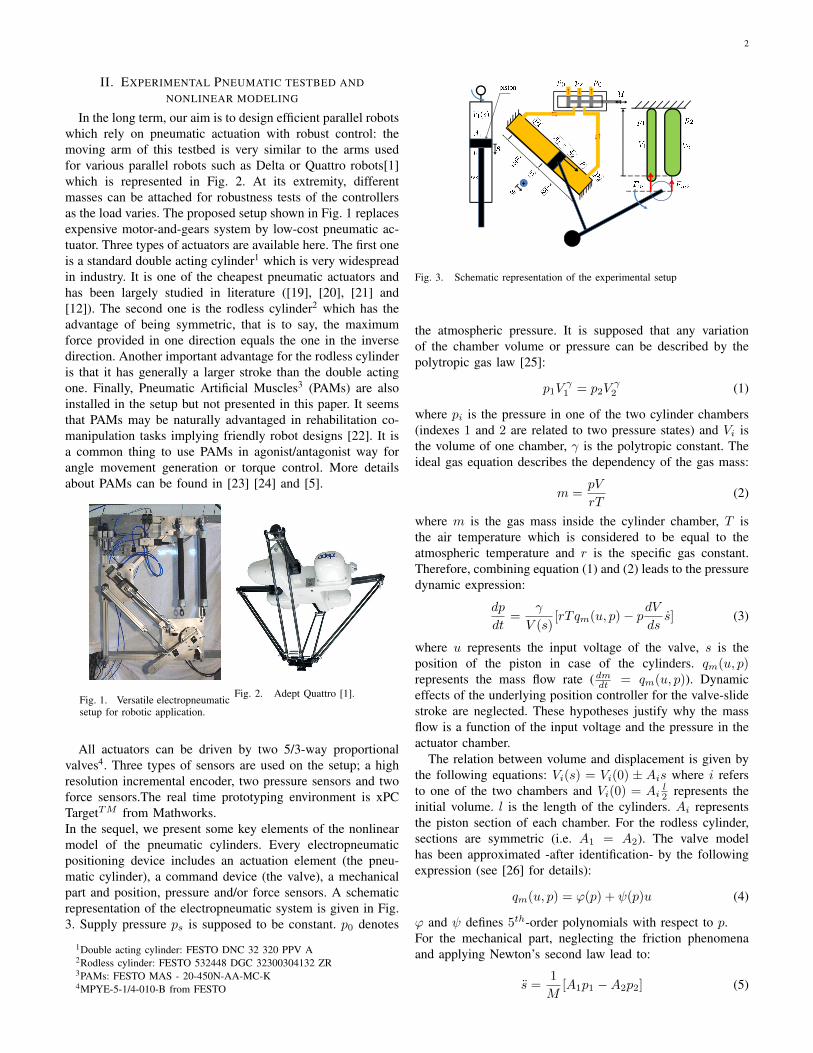
In the long term, our aim is to design efficient parallel robotswhich rely on pneumatic actuation with robust control: themoving arm of this testbed is very similar to the arms usedfor various parallel robots such as Delta or Quattro robots[1]which is represented in Fig. 2. At its extremity, differentmasses can be attached for robustness tests of the controllersas the load varies. The proposed setup shown in Fig. 1 replacesexpensive motor-and-gears system by low-cost pneumatic ac-tuator. Three types of actuators are available here. The first oneis a standard double acting cylinder1 which is very widespreadin industry. It is one of the cheapest pneumatic actuators andhas been largely studied in literature ([19], [20], [21] and[12]). The second one is the rodless cylinder2 which has theadvantage of being symmetric, that is to say, the maximumforce provided in one direction equals the one in the inversedirection. Another important advantage for the rodless cylinderis that it has generally a larger stroke than the double actingone. Finally, Pneumatic Artificial Muscles3 (PAMs) are alsoinstalled in the setup but not presented in this paper. It seemsthat PAMs may be naturally advantaged in rehabilitation co-manipulation tasks implying friendly robot designs [22]. It isa common thing to use PAMs in agonist/antagonist way forangle movement generation or torque control. More detailsabout PAMs can be found in [23] [24] and [5].

Fig. 1. Versatile electropneumaticsetup for robotic application.

Fig. 2. Adept Quattro [1].

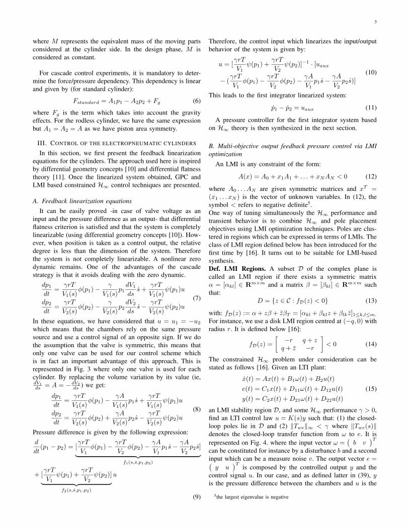
All actuators can be driven by two 5/3-way proportionalvalves4. Three types of sensors are used on the setup; a highresolution incremental encoder, two pressure sensors and twoforce sensors.The real time prototyping environment is xPCTargetTM from Mathworks.In the sequel, we present some key elements of the nonlinearmodel of the pneumatic cylinders. Every electropneumaticpositioning device includes an actuation element (the pneu-matic cylinder), a command device (the valve), a mechanicalpart and position, pressure and/or force sensors. A schematicrepresentation of the electropneumatic system is given in Fig.3. Supply pressure ps is supposed to be constant. p0 denotes

1Double acting cylinder: FESTO DNC 32 320 PPV A2Rodless cylinder: FESTO 532448 DGC 32300304132 ZR3PAMs: FESTO MAS - 20-450N-AA-MC-K4MPYE-5-1/4-010-B from FESTO

+

Fig. 3. Schematic representation of the experimental setup

the atmospheric pressure. It is supposed that any variationof the chamber volume or pressure can be described by thepolytropic gas law [25]:

p1Vγ1 = p2V

γ2 (1)

where pi is the pressure in one of the two cylinder chambers(indexes 1 and 2 are related to two pressure states) and Vi isthe volume of one chamber, γ is the polytropic constant. Theideal gas equation describes the dependency of the gas mass:

m =pV

rT(2)

where m is the gas mass inside the cylinder chamber, T isthe air temperature which is considered to be equal to theatmospheric temperature and r is the specific gas constant.Therefore, combining equation (1) and (2) leads to the pressuredynamic expression:

dp

dt=

γ

V (s)[rTqm(u, p)− pdV

dss] (3)

where u represents the input voltage of the valve, s is theposition of the piston in case of the cylinders. qm(u, p)represents the mass flow rate (dmdt = qm(u, p)). Dynamiceffects of the underlying position controller for the valve-slidestroke are neglected. These hypotheses justify why the massflow is a function of the input voltage and the pressure in theactuator chamber.

The relation between volume and displacement is given bythe following equations: Vi(s) = Vi(0) ± Ais where i refersto one of the two chambers and Vi(0) = Ai

l2 represents the

initial volume. l is the length of the cylinders. Ai representsthe piston section of each chamber. For the rodless cylinder,sections are symmetric (i.e. A1 = A2). The valve modelhas been approximated -after identification- by the followingexpression (see [26] for details):

qm(u, p) = ϕ(p) + ψ(p)u (4)

ϕ and ψ defines 5th-order polynomials with respect to p.For the mechanical part, neglecting the friction phenomenaand applying Newton’s second law lead to:

s =1

M[A1p1 −A2p2] (5)

3

where M represents the equivalent mass of the moving partsconsidered at the cylinder side. In the design phase, M isconsidered as constant.

For cascade control experiments, it is mandatory to deter-mine the force/pressure dependency. This dependency is linearand given by (for standard cylinder):

Fstandard = A1p1 −A2p2 + Fg (6)

where Fg is the term which takes into account the gravityeffects. For the rodless cylinder, we have the same expressionbut A1 = A2 = A as we have piston area symmetry.

III. CONTROL OF THE ELECTROPNEUMATIC CYLINDERS

In this section, we first present the feedback linearizationequations for the cylinders. The approach used here is inspiredby differential geometry concepts [10] and differential flatnesstheory [11]. Once the linearized system obtained, GPC andLMI based constrained H∞ control techniques are presented.

A. Feedback linearization equationsIt can be easily proved -in case of valve voltage as an

input and the pressure difference as an output- that differentialflatness criterion is satisfied and that the system is completelylinearizable (using differential geometry concepts [10]). How-ever, when position is taken as a control output, the relativedegree is less than the dimension of the system. Thereforethe system is not completely linearizable. A nonlinear zerodynamic remains. One of the advantages of the cascadestrategy is that it avoids dealing with the zero dynamic.

dp1dt

=γrT

V1(s)φ(p1)− γ

V1(s)p1dV1ds

s+γrT

V1(s)ψ(p1)u

dp2dt

=γrT

V2(s)φ(p2)− γ

V2(s)p2dV2ds

s− γrT

V2(s)ψ(p2)u

(7)

In these equations, we have considered that u = u1 = −u2which means that the chambers rely on the same pressuresource and use a control signal of an opposite sign. If we dothe assumption that the valve is symmetric, this means thatonly one valve can be used for our control scheme whichis in fact an important advantage of this approach. This isrepresented in Fig. 3 where only one valve is used for eachcylinder. By replacing the volume variation by its value (ie,dV1

ds = A = −dV2

ds ) we get:

dp1dt

=γrT

V1(s)φ(p1)− γA

V1(s)p1s+

γrT

V1(s)ψ(p1)u

dp2dt

=γrT

V2(s)φ(p2) +

γA

V2(s)p2s−

γrT

V2(s)ψ(p2)u

(8)

Pressure difference is given by the following expression:d

dt(p1 − p2) = [

γrT

V1φ(p1)− γrT

V2φ(p2)− γA

V1p1s−

γA

V2p2s]︸ ︷︷ ︸

f1(s,s,p1,p2)

+ [γrT

V1ψ(p1) +

γrT

V2ψ(p2)]︸ ︷︷ ︸

f2(s,s,p1,p2)

u

(9)

Therefore, the control input which linearizes the input/outputbehavior of the system is given by:

u = [γrT

V1ψ(p1) +

γrT

V2ψ(p2)]−1 · [uaux

− (γrT

V1φ(p1)− γrT

V2φ(p2)− γA

V1p1s−

γA

V2p2s)]

(10)

This leads to the first integrator linearized system:

p1 − p2 = uaux (11)

A pressure controller for the first integrator system basedon H∞ theory is then synthesized in the next section.

B. Multi-objective output feedback pressure control via LMIoptimization

An LMI is any constraint of the form:

A(x) = A0 + x1A1 + . . .+ xNAN < 0 (12)

where A0 . . . AN are given symmetric matrices and xT =(x1 . . . xN ) is the vector of unknown variables. In (12), thesymbol < refers to negative definite5.One way of tuning simultaneously the H∞ performance andtransient behavior is to combine H∞ and pole placementobjectives using LMI optimization techniques. Poles are clus-tered in regions which can be expressed in terms of LMIs. Theclass of LMI region defined below has been introduced for thefirst time by [16]. It turns out to be suitable for LMI-basedsynthesis.Def. LMI Regions. A subset D of the complex plane iscalled an LMI region if there exists a symmetric matrixα = [αkl] ∈ Rm×m and a matrix β = [βkl] ∈ Rm×m suchthat:

D = z ∈ C : fD(z) < 0 (13)

with: fD(z) := α+ zβ + zβT = [αkl + βklz + βlkz]1≤k,l≤m.For instance, we use a disk LMI region centred at (−q, 0) withradius r. It is defined below [16]:

fD(z) =

[−r q + zq + z −r

]< 0 (14)

The constrained H∞ problem under consideration can bestated as follows [16]. Given an LTI plant:

x(t) = Ax(t) +B1ω(t) +B2u(t)

e(t) = C1x(t) +D11ω(t) +D12u(t)

y(t) = C2x(t) +D21ω(t) +D22u(t)

(15)

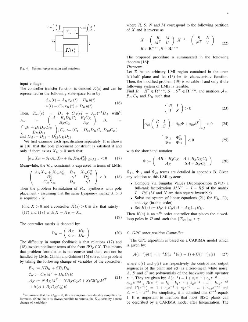
an LMI stability region D, and some H∞ performance γ > 0,find an LTI control law u = K(s)y such that: (1) the closed-loop poles lie in D and (2) ‖Twe‖∞ < γ where ‖Twe(s)‖denotes the closed-loop transfer function from ω to e. It isrepresented on Fig. 4. where the input vector ω =

(b v

)Tcan be constituted for instance by a disturbance b and a secondinput which can be a measure noise v. The output vector e =(y u

)Tis composed by the controlled output y and the

control signal u. In our case, and as defined latter in (39), yis the pressure difference between the chambers and u is the

5the largest eigenvalue is negative

4

Fig. 4. System representation and notations

input voltage.The controller transfer function is denoted K(s) and can berepresented in the following state-space form by:

xK(t) = AKxK(t) +BKy(t)

u(t) = CKxK(t) +DKy(t)(16)

Then, Twe(s) = Dcl + Ccl(sI − Acl)−1Bcl with6:

Acl :=

(A+B2DKC2 B2CK

BKC2 AK

), Bcl :=(

B1 +B2DKD21

BKD21

), Ccl := (C1 +D12DKC2, D12CK)

and Dcl := D11 +D12DKD21.We first examine each specification separately. It is shown

in [16] that the pole placement constraint is satisfied if andonly if there exists XD > 0 such that:

[αklXD + βklAclXD + βlkXDATcl]1≤k,l≤m < 0 (17)

Meanwhile, the H∞ constraint is expressed in terms of LMIs: AclX∞ +X∞ATcl Bcl X∞C

Tcl

BTcl −γI DTcl

CclX∞ Dcl −γI

< 0 (18)

Then the problem formulation of H∞ synthesis with poleplacement - assuming that the same Lyapunov matrix X > 0is required - is:

Find X > 0 and a controller K(s) > 0 ≡ ΩK that satisfy(17) and (18) with X = XD = X∞

(19)

The controller matrix is denoted by:

ΩK =

(AK BKCK DK

)(20)

The difficulty in output feedback is that relations (17) and(18) involve nonlinear terms of the form BΩKCX . This meansthat problem formulation is not convex and then, can not behandled by LMIs. Chilali and Gahinet [16] solved this problemby taking the following change of variables of the controller:

BK := NBK + SB2DK

CK := CKMT +DKC2R

AK := NAKMT +NBKC2R+ SB2CKM

T

+ S(A+B2DKC2)R

(21)

6we assume that the D22 = 0, this assumption considerably simplifies theformulas. (Note that it is always possible to remove the D22 term by a merechange of variables)

where R, S, N and M correspond to the following partitionof X and it inverse as

X =

(R MMT U

), X−1 =

(S NNT V

)R ∈ Rn×n, S ∈ Rn×n

(22)

The proposed procedure is summarized in the followingtheorem [16]:Theorem:Let D be an arbitrary LMI region contained in the openleft-half plane and let (13) be its characteristic function.Then, the modified problem (19) is solvable if and only if thefollowing system of LMIs is feasible.Find R = RT ∈ Rn×n, S = ST ∈ Rn×n, and matrices AK ,BK ,CK and DK such that(

R II S

)> 0 (23)

[αkl

(R II S

)+ βklΦ + βlkφ

T

]k,l

< 0 (24)

[Ψ11 ΨT

21

Ψ21 Ψ22

]< 0 (25)

with the shorthand notation

Φ :=

(AR+B2CK A+B2DKC2

AK SA+ BKC2

)(26)

Ψ11, Ψ12 and Ψ22 terms are detailed in appendix B. Givenany solution to this LMI system:

• Compute via Singular Values Decomposition (SVD) afull-rank factorization MNT = I − RS of the matrixI −RS (M and N are then square invertible)

• Solve the system of linear equations (21) for BK , CKand AK (in this order).

• Set K(s) := DK + CK(sI −AK)−1BK .

Then K(s) is an nth order controller that places the closed-loop poles in D and such that ‖Twe‖∞ < γ.

C. GPC outer position Controller

The GPC algorithm is based on a CARIMA model whichis given by:

A(z−1)y(t) = z−dB(z−1)u(t− 1) + C(z−1)e(t) (27)

where u(t) and y(t) are respectively the control and outputsequences of the plant and e(t) is a zero-mean white noise.A, B and C are polynomials of the backward shift operatorz−1. They are given by; A(z−1) = 1 +a1z

−1 +a2z−2 + ...+

anaz−na , B(z−1) = b0 + b1z

−1 + b2z−2 + ... + bnbz

−nb

and C(z−1) = 1 + c1z−1 + c2z

−2 + ... + cncz−nc and

4 = 1 − z−1. For simplicity, it is admitted that C−1 equals1. It is important to mention that most SISO plants canbe described by a CARIMA model after linearization. The

5

GPC algorithm consists in applying a control sequence thatminimizes a multistage cost function of the form:

J(N1, N2, Nu) =

N2∑j=N1

δ(j)[y(t+ j|t)− w(t+ j)]2

+

N2∑j=1

λ(j)[4u(t+ j − 1)]2

(28)

where y(t + j|t) is an optimum j step ahead prediction ofthe system output on data up to time t, N1 and N2 arethe minimum and maximum cost horizons, Nu is the controlhorizon, δ(j) and λ(j) are weighting sequences and w(t+ j)is the future reference trajectory.The minimization of cost function leads to a future controlsequence u(t), u(t+ 1), ... where the output y(t+ j) is closeto w(t+ j). Therefore, in order to optimize cost function, thebest optimal prediction of y(t+ j) (for N1 ≤ j ≤ N2) has tobe determined. This needs the introduction of the followingDiophantine equation:

1 = Aj(z−1)A(z−1) + z−jFj(z

−1) (29)

with A = 4A(z−1) and polynomials Ej and Fj are uniquelydefined with degrees j − 1 and na respectively. 4 is definedas 4 = 1− z−1By multiplying (27) by 4Ej(z−1)zj and considering (29), weobtain:

y(t+ j) =Fj(z−1)y(t) + Ej(z

−1)B(z−1)4u(t+ j − d− 1)

+ Ej(z−1)e(t+ j)

(30)

Since the noise terms in (30) are all in the future (this isbecause degree of polynomial Ej(z−1) = j − 1), the bestprediction of y(t+ j) is:

y(t+ j|t) = Gj(z−1)4u(t+ j − d− 1) +Fj(z

−1)y(t) (31)

where Gj(z−1) = Ej(z−1)B(z−1)

Polynomials Ej and Fj can merely be obtained recursively(demonstration can be found for instance in [27]).In the future, it will be referred only to N = N2 = Nu as theprediction horizon. N1 is chosen equal to 0.Let’s consider the following set of j ahead optimal predictions:

y(t+ d+ 1|t) = Gd+14u(t) + Fd+1y(t)

...y(t+ d+N |t) = Gd+N4u(t+N − 1) + Fd+Ny(t)

(32)

It can be written in the following compact form:

y = G u + F(z−1)y(t) + G′(z−1)4u(t− 1) (33)

where terms y, u, G′ and F can be defined in [28].Equation (33) can be rewritten in this form:

y = Gu + f (34)

Where f refers to the last two terms in Eq. (33) which onlydepend on the past. Now, we are able to rewrite (28) as:

J = (Gu + f− w)T (Gu + f− w) + λuTu (35)

where w = [w(t + d + 1), w(t + d + 1) . . . w(t + d + N)]T

equation (35) can be written as:

J =1

2uTHu + bTu + f0 (36)

with H = 2(GTG + λI), bT = 2(f − w)TG and f0 =(f −w)T(f −w)Therefore, the minimum of J can simply be found by makingthe gradient of J equal to zero, which leads to:

u = −H−1b = (GTG + λI)−1GT(w − f) (37)

Since the control signal that is actually sent to the process isthe first element of vector u (receding strategy), it is given by:

4u(t) = K(w − f) (38)

where K represents the first element of matrix (GTG +λI)−1GT. Contrary to conventional controllers, predictiveones depend only on future errors and not past ones.

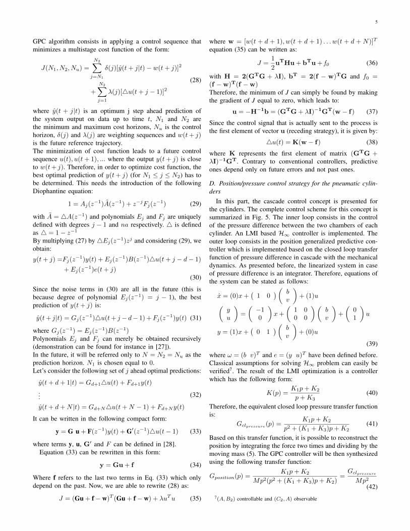
D. Position/pressure control strategy for the pneumatic cylin-ders

In this part, the cascade control concept is presented forthe cylinders. The complete control scheme for this concept issummarized in Fig. 5. The inner loop consists in the controlof the pressure difference between the two chambers of eachcylinder. An LMI based H∞ controller is implemented. Theouter loop consists in the position generalized predictive con-troller which is implemented based on the closed loop transferfunction of pressure difference in cascade with the mechanicaldynamics. As presented before, the linearized system in caseof pressure difference is an integrator. Therefore, equations ofthe system can be stated as follows:

x = (0)x+(

1 0)( b

v

)+ (1)u(

yu

)=

(−10

)x+

(1 00 0

)(bv

)+

(01

)u

y = (1)x+(

0 1)( b

v

)+ (0)u

(39)

where ω = (b v)T and e = (y u)T have been defined before.Classical assumptions for solving H∞ problem can easily beverified7. The result of the LMI optimization is a controllerwhich has the following form:

K(p) =K1p+K2

p+K3(40)

Therefore, the equivalent closed loop pressure transfer functionis:

Gclpressure(p) =

K1p+K2

p2 + (K1 +K3)p+K2(41)

Based on this transfer function, it is possible to reconstruct theposition by integrating the force two times and dividing by themoving mass (5). The GPC controller will be then synthesizedusing the following transfer function:

Gposition(p) =K1p+K2

Mp2(p2 + (K1 +K3)p+K2)=Gclpressure

Mp2(42)

7(A,B2) controllable and (C2, A) observable

6

I/O linearizing GPC

predictive controller Section

Desiredfutureangle

controller

Difference pressure inner GPC

parameters

Predictive position outer loop

CylinderValveI/O linearizing

block

Inverse kinematics

Difference pressure inner loop

Fig. 5. General block diagram of the cascade Position/pressure strategy for the cylinders. The inner loop consists in the control of the pressure differencebetween the two chambers of each cylinder. An LMI based H∞ controller is implemented. The outer loop consists in the position generalized predictivecontroller which is implemented based on the closed loop transfer function of pressure difference in cascade with the mechanical inverse dynamics.

IV. EXPERIMENTAL RESULTS

In the following, the proposed cascade GPC/H∞ is imple-mented on the pneumatic cylinders. Some typical tests arehandled and commented in details.

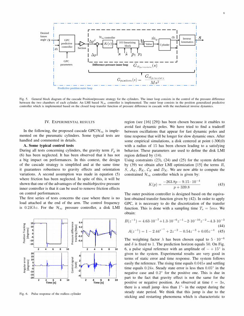
A. Some typical control testsDuring all tests concerning cylinders, the gravity term Fg in(6) has been neglected. It has been observed that it has nota big impact on performances. In this context, the designof the cascade strategy is simplified and at the same timeit guarantees robustness to gravity effects and orientationvariations. A second assumption was made in equation (5)where friction has been neglected. In spite of this, it will beshown that one of the advantages of the multiobjective pressureinner controller is that it can be used to remove friction effectson control performances.The first series of tests concerns the case where there is noload attached at the end of the arm. The control frequencyis 0.2Khz. For the H∞ pressure controller, a disk LMI

2 4 6 8 10

-15-10-505

1015

Po

siti

on

Tra

ckin

g

[de

gre

es]

2 4 6 8 10

-0.4

-0.2

0

0.2

0.4

Pre

ssu

re d

iffe

ren

ce

tra

ckin

g [

Mp

a]

2 4 6 8 10-20-15-10-505

101520

An

gu

lar

err

or

[de

gre

es]

Time [s]2 4 6 8 10

-4

-2

0

2

4

Co

ntr

ol

sig

na

l

[Vo

lt]

Time [s]

Fig. 6. Pulse response of the rodless cylinder

region (see [16] [29]) has been chosen because it enables toavoid fast dynamic poles. We have tried to find a tradeoffbetween oscillations that appear for fast dynamic poles andtime response that will be longer for slow dynamic ones. Aftersome empirical simulations, a disk centered at point (-300,0)with a radius of 15 has been chosen leading to a satisfyingbehavior. These parameters are used to define the disk LMIregion defined by (14).Using constraints (23), (24) and (25) for the system definedby (39) we obtain after LMI optimization [15] the terms R,S, AK , BK , CK and DK . We are now able to compute theconstrained H∞ controller which is given by:

K(p) =−263.8p− 9.15 · 10−4

p+ 339.8(43)

The outer position controller is designed based on the equiva-lent obtained transfer function given by (42). In order to applyGPC, it is necessary to do the discretization of the transferfunction. This is done with a sampling time Ts = 5ms. Weobtain:

B(z−1) = 4.63·10−7+1.3·10−6z−1−2·10−10z−2−4.3·10−3

(44)A(z−1) = 1− 2.44z

−1

+ 2z−2 − 0.54z−3 + 0.05z−4 (45)

The weighting factor λ has been chosen equal to 5 · 10−6

and δ is fixed to 1. The prediction horizon equals 50. On Fig.6, a pulse signal reference with an amplitude of − + 15 isgiven to the system. Experimental results are very good interms of static error and time response. The system followseasily the reference. The rising time equals 0.045s and settlingtime equals 0.24s. Steady state error is less then 0.05 in thenegative case and 0.2 for the positive one. This is due inpart to the fact that gravity effect is not the same for thepositive or negative position. As observed at time t = 3s,there is a small jump -less than 1- in the output during thesteady state period. We think that this jump is due to thesticking and restarting phenomena which is characteristic to

7

electropneumatic systems (see chapter 3 of [12]). In our case,our aim is to reach a precision better than 1 for carrying loadsup to 5kg in pick-and-place applications. This is achieved inall the tests presented in this document even in presence ofrestarting phenomena. However, this problem can be removedby changing the closed loop pole location of the inner pressurecontroller. For instance, rather than a circle LMI region ofradius 25 and centered at point (−350, 0), we constrain thepoles to be at (−450, 0). This is represented on figure 7.The consequence can be viewed on Fig. 8. The limit cycle

1st LMI region

zeros

Closed loop

poles

Ima

gin

ary

ax

is

2nd LMI

region

Ima

gin

ary

ax

is

Real axis

Closed loop

poles

Fig. 7. Zero pole map: LMI circle regions and closed loop pole location

1 2 3 4 5 6 7 8 9

-20

-15

-10

-5

0

Po

siti

on

Tra

ckin

g

[de

gre

es]

Reference signal

Output position signal

Time [s]

Fig. 8. High gain step response

has been completely removed. The steady state error equals0.02.

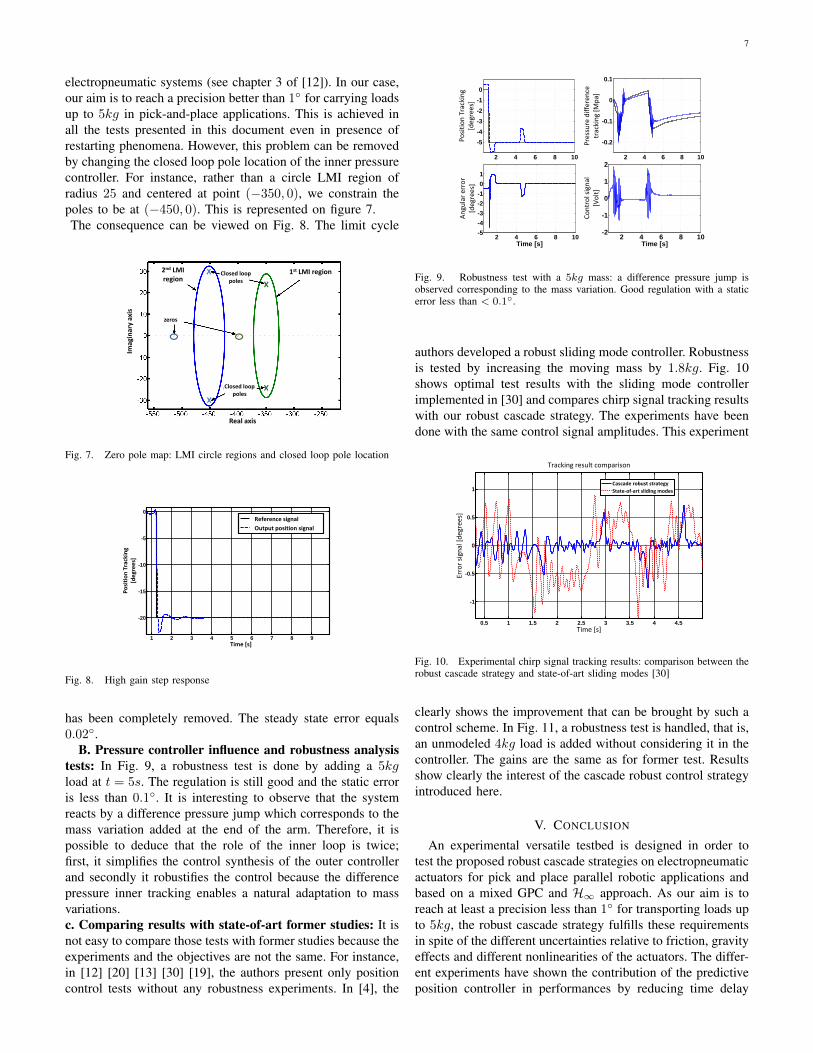
B. Pressure controller influence and robustness analysistests: In Fig. 9, a robustness test is done by adding a 5kgload at t = 5s. The regulation is still good and the static erroris less than 0.1. It is interesting to observe that the systemreacts by a difference pressure jump which corresponds to themass variation added at the end of the arm. Therefore, it ispossible to deduce that the role of the inner loop is twice;first, it simplifies the control synthesis of the outer controllerand secondly it robustifies the control because the differencepressure inner tracking enables a natural adaptation to massvariations.c. Comparing results with state-of-art former studies: It isnot easy to compare those tests with former studies because theexperiments and the objectives are not the same. For instance,in [12] [20] [13] [30] [19], the authors present only positioncontrol tests without any robustness experiments. In [4], the

2 4 6 8 10

-5

-4

-3

-2

-1

0

Po

siti

on

Tra

ckin

g

[de

gre

es]

2 4 6 8 10

-0.2

-0.1

0

0.1

Pre

ssu

re d

iffe

ren

ce

tra

ckin

g [

Mp

a]

2 4 6 8 10-5

-4

-3

-2

-1

0

1

An

gu

lar

err

or

[de

gre

es]

Time [s]2 4 6 8 10

-2

-1

0

1

2

Co

ntr

ol

sig

na

l

[Vo

lt]

Time [s]

Fig. 9. Robustness test with a 5kg mass: a difference pressure jump isobserved corresponding to the mass variation. Good regulation with a staticerror less than < 0.1.

authors developed a robust sliding mode controller. Robustnessis tested by increasing the moving mass by 1.8kg. Fig. 10shows optimal test results with the sliding mode controllerimplemented in [30] and compares chirp signal tracking resultswith our robust cascade strategy. The experiments have beendone with the same control signal amplitudes. This experiment

0.5 1 1.5 2 2.5 3 3.5 4 4.5

-1

-0.5

0

0.5

1

Tracking result comparison

Time [s]

Err

or

sig

na

l [d

eg

ree

s]

Cascade robust strategy

State-of-art sliding modes

Fig. 10. Experimental chirp signal tracking results: comparison between therobust cascade strategy and state-of-art sliding modes [30]

clearly shows the improvement that can be brought by such acontrol scheme. In Fig. 11, a robustness test is handled, that is,an unmodeled 4kg load is added without considering it in thecontroller. The gains are the same as for former test. Resultsshow clearly the interest of the cascade robust control strategyintroduced here.

V. CONCLUSION

An experimental versatile testbed is designed in order totest the proposed robust cascade strategies on electropneumaticactuators for pick and place parallel robotic applications andbased on a mixed GPC and H∞ approach. As our aim is toreach at least a precision less than 1 for transporting loads upto 5kg, the robust cascade strategy fulfills these requirementsin spite of the different uncertainties relative to friction, gravityeffects and different nonlinearities of the actuators. The differ-ent experiments have shown the contribution of the predictiveposition controller in performances by reducing time delay

8

0.5 1 1.5 2 2.5 3 3.5 4 4.5 5

-1.5

-1

-0.5

0

0.5

1

Robustness tracking result comparison

Time [s]

Err

or

sig

na

l [d

eg

ree

s]

Cascade robust strategy

State-of-art sliding modes

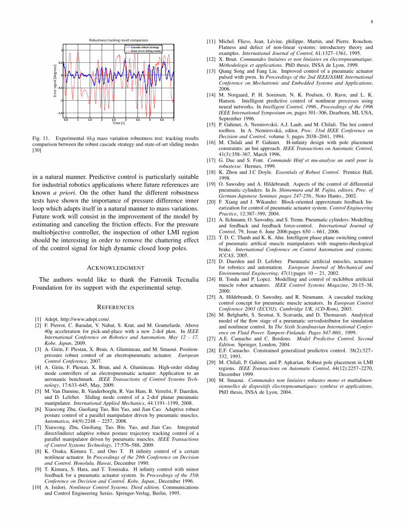
Fig. 11. Experimental 4kg mass variation robustness test: tracking resultscomparison between the robust cascade strategy and state-of-art sliding modes[30]

in a natural manner. Predictive control is particularly suitablefor industrial robotics applications where future references areknown a priori. On the other hand the different robustnesstests have shown the importance of pressure difference innerloop which adapts itself in a natural manner to mass variations.Future work will consist in the improvement of the model byestimating and canceling the friction effects. For the pressuremultiobjective controller, the inspection of other LMI regionshould be interesting in order to remove the chattering effectof the control signal for high dynamic closed loop poles.

ACKNOWLEDGMENT

The authors would like to thank the Fatronik TecnaliaFoundation for its support with the experimental setup.

REFERENCES

[1] Adept, http://www.adept.com/.[2] F. Pierrot, C. Baradat, V. Nabat, S. Krut, and M. Gouttefarde. Above

40g acceleration for pick-and-place with a new 2-dof pkm. In IEEEInternational Conference on Robotics and Automation, May 12 - 17,Kobe, Japan, 2009.

[3] A. Girin, F. Plestan, X. Brun, A. Glumineau, and M. Smaoui. Position-pressure robust control of an electropneumatic actuator. EuropeanControl Conference, 2007.

[4] A. Girin, F. Plestan, X. Brun, and A. Glumineau. High-order slidingmode controllers of an electropneumatic actuator: Application to anaeronautic benchmark. IEEE Transactions of Control Systems Tech-nology, 17:633–645, May, 2009.

[5] M. Van Damme, B. Vanderborght, R. Van Ham, B. Verrelst, F. Daerden,and D. Lefeber. Sliding mode control of a 2-dof planar pneumaticmanipulator. International Applied Mechanics, 44:1191–1199, 2008.

[6] Xiaocong Zhu, Guoliang Tao, Bin Yao, and Jian Cao. Adaptive robustposture control of a parallel manipulator driven by pneumatic muscles.Automatica, 44(9):2248 – 2257, 2008.

[7] Xiaocong. Zhu, Guoliang. Tao, Bin. Yao, and Jian Cao. Integrateddirect/indirect adaptive robust posture trajectory tracking control of aparallel manipulator driven by pneumatic muscles. IEEE Transactionsof Control Systems Technology, 17:576–588, 2009.

[8] K. Osuka, Kimura T., and Ono T. H infinity control of a certainnonlinear actuator. In Proceedings of the 29th Conference on Decisionand Control. Honolulu, Hawai, December 1990.

[9] T. Kimura, S. Hara, and T. Tomisaka. H infinity control with minorfeedback for a pneumatic actuator system. In Proceedings of the 35thConference on Decision and Control. Kobe, Japan., December 1996.

[10] A. Isidori. Nonlinear Control Systems. Third edition. Communicationsand Control Engineering Series. Springer-Verlag, Berlin, 1995.

[11] Michel. Fliess, Jean. Levine, philippe. Martin, and Pierre. Rouchon.Flatness and defect of non-linear systems: introductory theory andexamples. International Journal of Control, 61:1327–1361, 1995.

[12] X. Brun. Commandes lineaires et non lineaires en electropneumatique.Methodologie et applications. PhD thesis, INSA de Lyon, 1999.

[13] Qiang Song and Fang Liu. Improved control of a pneumatic actuatorpulsed with pwm. In Proceedings of the 2nd IEEE/ASME InternationalConference on Mechatronic and Embedded Systems and Applications,2006.

[14] M. Norgaard, P. H. Sorensen, N. K. Poulsen, O. Ravn, and L. K.Hansen. Intelligent predictive control of nonlinear processes usingneural networks. In Intelligent Control, 1996., Proceedings of the 1996IEEE International Symposium on, pages 301–306, Dearborn, MI, USA,September 1996.

[15] P. Gahinet, A. Nemirovskii, A.J. Laub, and M. Chilali. The lmi controltoolbox. In A. Nemirovskii, editor, Proc. 33rd IEEE Conference onDecision and Control, volume 3, pages 2038–2041, 1994.

[16] M. Chilali and P. Gahinet. H-infinity design with pole placementconstraints: an lmi approach. IEEE Transactions on Automatic Control,41(3):358–367, March 1996.

[17] G. Duc and S. Font. Commande Hinf et mu-analyse un outil pour larobustesse. Hermes, 1999.

[18] K. Zhou and J.C Doyle. Essentials of Robust Control. Prentice Hall,1998.

[19] O. Sawodny and A. Hildebrandt. Aspects of the control of differentialpneumatic cylinders. In In. Shimemura and M. Fujita, editors, Proc. ofGerman-Japanese Seminar, pages 247-256., Noto Hanto., 2002.

[20] F. Xiang and J. Wikander. Block-oriented approximate feedback lin-earization for control of pneumatic actuator system. Control EngineeringPractice, 12:387–399, 2004.

[21] A. Ilchmann, O. Sawodny, and S. Trenn. Pneumatic cylinders: Modellingand feedback and feedback force-control. International Journal ofControl, 79, Issue 6. June 2006:pages 650 – 661, 2006.

[22] T. D. C. Thanh and K. K. Ahn. Intelligent phase plane switching controlof pneumatic artifical muscle manipulators with magneto-rheologicalbrake. International Conference on Control Automation and systems,ICCAS, 2005.

[23] D. Daerden and D. Lefeber. Pneumatic artificial muscles, actuatorsfor robotics and automation. European Journal of Mechanical andEnvironmental Engineering, 47(1):pages 10 – 21, 2002.

[24] B. Tondu and P. Lopez. Modelling and control of mckibben artificialmuscle robot actuators. IEEE Control Systems Magazine, 20:15–38,2000.

[25] A. Hildebrandt, O. Sawodny, and R. Neumann. A cascaded trackingcontrol concept for pneumatic muscle actuators. In European ControlConference 2003 (ECC03), Cambridge UK, (CD-Rom), 2003.

[26] M. Belgharbi, S. Sesmat, S. Scavarda, and D. Thomasset. Analyticalmodel of the flow stage of a pneumatic servodistributor for simulationand nonlinear control. In The Sixth Scandinavian International Confer-ence on Fluid Power. Tampere-Finlande. Pages 847-860., 1999.

[27] A.E. Camacho and C. Bordons. Model Predicitve Control. SecondEdition. Springer, London, 2004.

[28] E.F. Camacho. Constrained generalized predictive control. 38(2):327–332, 1993.

[29] M. Chilali, P. Gahinet, and P. Apkarian. Robust pole placement in LMIregions. IEEE Transactions on Automatic Control, 44(12):2257–2270,December 1999.

[30] M. Smaoui. Commandes non lineaires robustes mono et multidimen-sionnelles de dispositifs electropneumatiques: synthese et applications.PhD thesis, INSA de Lyon, 2004.