A Minimum Relative Entropy Principle for Learning and Acting · way out of an unknown maze and designing an autonomous robot for Martian exploration. Adaptive control turns out to

Journal of Artificial Intelligence Research 38 (2010) 475-511 Submitted 04/10; published 08/10

A Minimum Relative Entropy Principlefor Learning and Acting

Pedro A. Ortega [email protected]

Daniel A. Braun [email protected]

Department of Engineering

University of Cambridge

Cambridge CB2 1PZ, UK

Abstract

This paper proposes a method to construct an adaptive agent that is universal withrespect to a given class of experts, where each expert is designed specifically for a particularenvironment. This adaptive control problem is formalized as the problem of minimizingthe relative entropy of the adaptive agent from the expert that is most suitable for theunknown environment. If the agent is a passive observer, then the optimal solution is thewell-known Bayesian predictor. However, if the agent is active, then its past actions needto be treated as causal interventions on the I/O stream rather than normal probabilityconditions. Here it is shown that the solution to this new variational problem is givenby a stochastic controller called the Bayesian control rule, which implements adaptivebehavior as a mixture of experts. Furthermore, it is shown that under mild assumptions,the Bayesian control rule converges to the control law of the most suitable expert.

1. Introduction

When the behavior of an environment under any control signal is fully known, then thedesigner can choose an agent that produces the desired dynamics. Instances of this prob-lem include hitting a target with a cannon under known weather conditions, solving a mazehaving its map and controlling a robotic arm in a manufacturing plant. However, whenthe environment is unknown, then the designer faces the problem of adaptive control. Forexample, shooting the cannon lacking the appropriate measurement equipment, finding theway out of an unknown maze and designing an autonomous robot for Martian exploration.Adaptive control turns out to be far more difficult than its non-adaptive counterpart. Thisis because any good policy has to carefully trade off explorative versus exploitative actions,i.e. actions for the identification of the environment’s dynamics versus actions to control itin a desired way. Even when the environment’s dynamics are known to belong to a partic-ular class for which optimal agents are available, constructing the corresponding optimaladaptive agent is in general computationally intractable even for simple toy problems (Duff,2002). Thus, finding tractable approximations has been a major focus of research.

Recently, it has been proposed to reformulate the problem statement for some classes ofcontrol problems based on the minimization of a relative entropy criterion. For example, alarge class of optimal control problems can be solved very efficiently if the problem statementis reformulated as the minimization of the deviation of the dynamics of a controlled systemfrom the uncontrolled system (Todorov, 2006, 2009; Kappen, Gomez, & Opper, 2010). Inthis work, a similar approach is introduced for adaptive control. If a class of agents is

c©2010 AI Access Foundation. All rights reserved.

475

Ortega & Braun

given, where each agent is tailored to a different environment, then adaptive controllers canbe derived from a minimum relative entropy principle. In particular, one can construct anadaptive agent that is universal with respect to this class by minimizing the average relativeentropy from the environment-specific agent.

However, this extension is not straightforward. There is a syntactical difference betweenactions and observations that has to be taken into account when formulating the variationalproblem. More specifically, actions have to be treated as interventions obeying the rules ofcausality (Pearl, 2000; Spirtes, Glymour, & Scheines, 2000; Dawid, 2010). If this distinctionis made, the variational problem has a unique solution given by a stochastic control rulecalled the Bayesian control rule. This control rule is particularly interesting because ittranslates the adaptive control problem into an on-line inference problem that can be appliedforward in time. Furthermore, this work shows that under mild assumptions, the adaptiveagent converges to the environment-specific agent.

The paper is organized as follows. Section 2 introduces notation and sets up the adaptivecontrol problem. Section 3 formulates adaptive control as a minimum relative entropyproblem. After an initial, naıve approach, the need for causal considerations is motivated.Then, the Bayesian control rule is derived from a revised relative entropy criterion. InSection 4, the conditions for convergence are examined and a proof is given. Section 5illustrates the usage of the Bayesian control rule for the multi-armed bandit problem andundiscounted Markov decision processes. Section 6 discusses properties of the Bayesiancontrol rule and relates it to previous work in the literature. Section 7 concludes.

2. Preliminaries

In the following both agent and environment are formalized as causal models over I/Osequences. Agent and environment are coupled to exchange symbols following a standardinteraction protocol having discrete time, observation and control signals. The treatmentof the dynamics are fully probabilistic, and in particular, both actions and observations arerandom variables, which is in contrast to the typical decision-theoretic agent formulationtreating only observations as random variables (Russell & Norvig, 2010). All proofs areprovided in the appendix.

Notation. A set is denoted by a calligraphic letter like A. The words set & alphabetand element & symbol are used to mean the same thing respectively. Strings are finiteconcatenations of symbols and sequences are infinite concatenations. An denotes the setof strings of length n based on A, and A∗ :=

⋃n≥0 A

n is the set of finite strings. Fur-thermore, A∞ := {a1a2 . . . |ai ∈ A for all i = 1, 2, . . .} is defined as the set of one-wayinfinite sequences based on the alphabet A. Tuples are written with parentheses (a1, a2, a3)or as strings a1a2a3. The notation a≤i := a1a2 . . . ai is a shorthand for a string start-ing from the first index. Also, symbols are underlined to glue them together like ao inao≤i := a1o1a2o2 . . . aioi. The function log(x) is meant to be taken w.r.t. base 2, unlessindicated otherwise.

Interactions. The possible I/O symbols are drawn from two finite sets. Let O denote theset of inputs (observations) and let A denote the set of outputs (actions). The set Z := A×Ois the interaction set. A string ao≤t or ao<tat is an interaction string (optionally ending in

476

A Minimum Relative Entropy Principle for Learning and Acting

at or ot) where ak ∈ A and ok ∈ O. Similarly, a one-sided infinite sequence a1o1a2o2 . . . isan interaction sequence. The set of interaction strings of length t is denoted by Zt. Thesets of (finite) interaction strings and sequences are denoted as Z∗ and Z∞ respectively.The interaction string of length 0 is denoted by ε.

I/O System. Agents and environments are formalized as I/O systems. An I/O systemis a probability distribution Pr over interaction sequences Z∞. Pr is uniquely determinedby the conditional probabilities

Pr(at|ao<t), Pr(ot|ao<tat) (1)

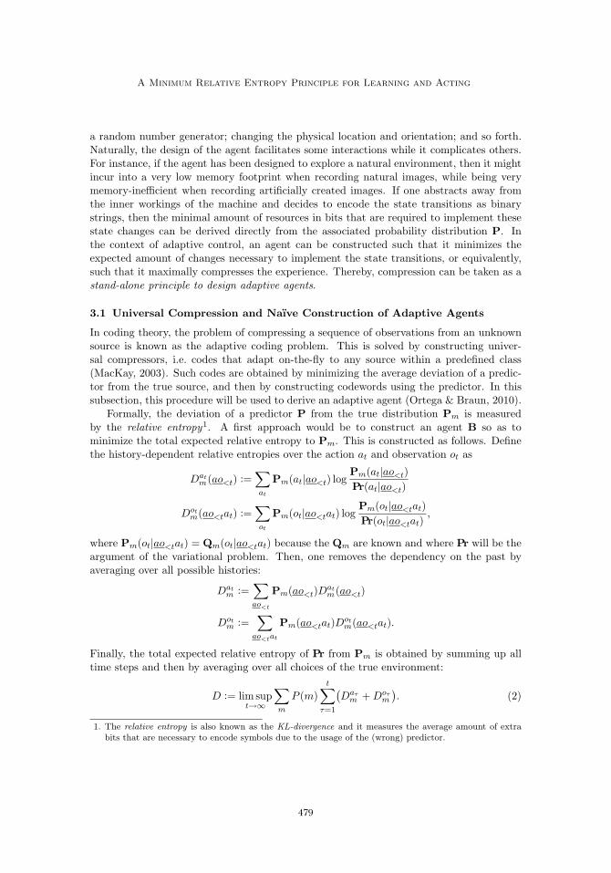
for each ao≤t ∈ Z∗. These conditional probabilities can either represent a generative law(“propensity”) in case of issuing a symbol or an evidential probability (“plausibility”) in thecase of observing a symbol. Which of the two interpretations applies in a particular casebecomes apparent once the I/O system is coupled to another I/O system.

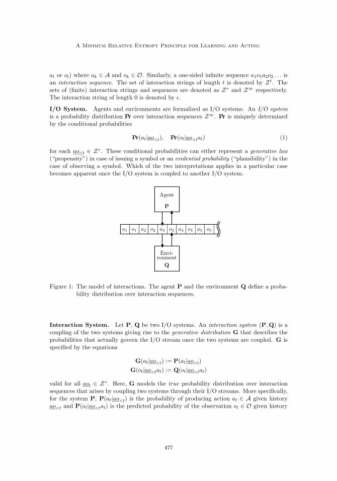
a1 a2 a3 a4 a5o1 o2 o3 o4 o5

Agent

P

Envi-ronment

Q

Figure 1: The model of interactions. The agent P and the environment Q define a proba-bility distribution over interaction sequences.

Interaction System. Let P, Q be two I/O systems. An interaction system (P,Q) is acoupling of the two systems giving rise to the generative distribution G that describes theprobabilities that actually govern the I/O stream once the two systems are coupled. G isspecified by the equations

G(at|ao<t) := P(at|ao<t)

G(ot|ao<tat) := Q(ot|ao<tat)

valid for all aot ∈ Z∗. Here, G models the true probability distribution over interactionsequences that arises by coupling two systems through their I/O streams. More specifically,for the system P, P(at|ao<t) is the probability of producing action at ∈ A given historyao<t and P(ot|ao<tat) is the predicted probability of the observation ot ∈ O given history

477

Ortega & Braun

ao<tat. Hence, for P, the sequence o1o2 . . . is its input stream and the sequence a1a2 . . .is its output stream. In contrast, the roles of actions and observations are reversed in thecase of the system Q. Thus, the sequence o1o2 . . . is its output stream and the sequencea1a2 . . . is its input stream. The previous model of interaction is fairly general, and manyother interaction protocols can be translated into this scheme. As a convention, given aninteraction system (P,Q), P is an agent to be constructed by the designer, and Q is anenvironment to be controlled by the agent. Figure 1 illustrates this setup.

Control Problem. An environment Q is said to be known iff the agent P has the propertythat for any ao≤t ∈ Z∗,

P(ot|ao<tat) = Q(ot|ao<tat).

Intuitively, this means that the agent “knows” the statistics of the environment’s futurebehavior under any past, and in particular, it “knows” the effects of given controls. If theenvironment is known, then the designer of the agent can build a custom-made policy intoP such that the resulting generative distribution G produces interaction sequences that aredesirable. This can be done in multiple ways. For instance, the controls can be chosensuch that the resulting policy maximizes a given utility criterion; or such that the resultingtrajectory of the interaction system stays close enough to a prescribed trajectory. Formally,if Q is known, and if the conditional probabilities P(at|ao<t) for all ao≤t ∈ Z∗ have beenchosen such that the resulting generative distribution G over interaction sequences givenby

G(at|ao<t) = P(at|ao<t)

G(ot|ao<tat) = Q(ot|ao<tat) = P(ot|ao<tat)

is desirable, then P is said to be tailored to Q.

Adaptive Control Problem. If the environment Q is unknown, then the task of de-signing an appropriate agent P constitutes an adaptive control problem. Specifically, thiswork deals with the case when the designer already has a class of agents that are tailoredto the class of possible environments. Formally, it is assumed that Q is going to be drawnwith probability P (m) from a set Q := {Qm}m∈M of possible systems before the inter-action starts, where M is a countable set. Furthermore, one has a set P := {Pm}m∈M

of systems such that for each m ∈ M, Pm is tailored to Qm and the interaction system(Pm,Qm) has a generative distribution Gm that produces desirable interaction sequences.How can the designer construct a system P such that its behavior is as close as possible tothe custom-made system Pm under any realization of Qm ∈ Q?

3. Adaptive Systems

The main goal of this paper is to show that the problem of adaptive control outlined inthe previous section can be reformulated as a universal compression problem. This can beinformally motivated as follows. Suppose the agent P is implemented as a machine that isinterfaced with the environment Q. Whenever the agent interacts with the environment,the agent’s state changes as a necessary consequence of the interaction. This “change instate” can take place in many possible ways: by updating the internal memory; consulting

478


a random number generator; changing the physical location and orientation; and so forth.Naturally, the design of the agent facilitates some interactions while it complicates others.For instance, if the agent has been designed to explore a natural environment, then it mightincur into a very low memory footprint when recording natural images, while being verymemory-inefficient when recording artificially created images. If one abstracts away fromthe inner workings of the machine and decides to encode the state transitions as binarystrings, then the minimal amount of resources in bits that are required to implement thesestate changes can be derived directly from the associated probability distribution P. Inthe context of adaptive control, an agent can be constructed such that it minimizes theexpected amount of changes necessary to implement the state transitions, or equivalently,such that it maximally compresses the experience. Thereby, compression can be taken as astand-alone principle to design adaptive agents.

3.1 Universal Compression and Naıve Construction of Adaptive Agents

In coding theory, the problem of compressing a sequence of observations from an unknownsource is known as the adaptive coding problem. This is solved by constructing univer-sal compressors, i.e. codes that adapt on-the-fly to any source within a predefined class(MacKay, 2003). Such codes are obtained by minimizing the average deviation of a predic-tor from the true source, and then by constructing codewords using the predictor. In thissubsection, this procedure will be used to derive an adaptive agent (Ortega & Braun, 2010).

Formally, the deviation of a predictor P from the true distribution Pm is measuredby the relative entropy1. A first approach would be to construct an agent B so as tominimize the total expected relative entropy to Pm. This is constructed as follows. Definethe history-dependent relative entropies over the action at and observation ot as

Dat

m(ao<t) :=∑at

Pm(at|ao<t) logPm(at|ao<t)

Pr(at|ao<t)

Dot

m(ao<tat) :=∑ot

Pm(ot|ao<tat) logPm(ot|ao<tat)

Pr(ot|ao<tat),

where Pm(ot|ao<tat) = Qm(ot|ao<tat) because the Qm are known and where Pr will be theargument of the variational problem. Then, one removes the dependency on the past byaveraging over all possible histories:

Dat

m :=∑ao

<t

Pm(ao<t)Dat

m(ao<t)

Dot

m :=∑

ao<t

at

Pm(ao<tat)Dot

m(ao<tat).

Finally, the total expected relative entropy of Pr from Pm is obtained by summing up alltime steps and then by averaging over all choices of the true environment:

D := lim supt→∞

∑m

P (m)t∑

τ=1

(Daτ

m + Doτ

m

). (2)

1. The relative entropy is also known as the KL-divergence and it measures the average amount of extrabits that are necessary to encode symbols due to the usage of the (wrong) predictor.

479

Ortega & Braun

Using (2), one can define a variational problem with respect to Pr. The agent B that oneis looking for is the system Pr that minimizes the total expected relative entropy in (2), i.e.

B := arg minPr

D(Pr). (3)

The solution to Equation 3 is the system B defined by the set of equations

B(at|ao<t) =∑m

Pm(at|ao<t)wm(ao<t)

B(ot|ao<tat) =∑m

Pm(ot|ao<tat)wm(ao<tat)(4)

valid for all ao≤t ∈ Z∗, where the mixture weights are

wm(ao<t) :=P (m)Pm(ao<t)∑

m′ P (m′)Pm′(ao<t)

wm(ao<tat) :=P (m)Pm(ao<tat)∑

m′ P (m′)Pm′(ao<tat).

(5)

For reference, see the work of Haussler and Opper (1997) and Opper (1998). It is clearthat B is just the Bayesian mixture over the agents Pm. If one defines the conditionalprobabilities

P (at|m, ao<t) := Pm(at|ao<t)

P (ot|m, ao<tat) := Pm(at|ao<tat)(6)

for all ao≤t ∈ Z∗, then Equation 4 can be rewritten as

B(at|ao<t) =∑m

P (at|m, ao<t)P (m|ao<t) = P (at|ao<t)

B(ot|ao<tat) =∑m

P (ot|m, ao<tat)P (m|ao<tat) = P (ot|ao<tat)(7)

where the P (m|ao<t) = wm(ao<t) and P (m|ao<tat) = wm(ao<tat) are just the posteriorprobabilities over the elements in M given the past interactions. Hence, the conditionalprobabilities in (4) that minimize the total expected divergence are just the predictivedistributions P (at|ao<t) and P (ot|ao<tat) that one obtains by standard probability theory,and in particular, Bayes’ rule. This is interesting, as it provides a teleological interpretationfor Bayes’ rule.

The behavior of B can be described as follows. At any given time t, B maintains amixture over systems Pm. The weighting over them is given by the mixture coefficientswm. Whenever a new action at or a new observation ot is produced (by the agent orthe environment respectively), the weights wm are updated according to Bayes’ rule. Inaddition, B issues an action at suggested by a system Pm drawn randomly according to theweights wt.

However, there is an important problem with B that arises due to the fact that it is notonly a system that is passively observing symbols, but also actively generating them. Inthe subjective interpretation of probability theory, conditionals play the role of observations

480


made by the agent that have been generated by an external source. This interpretation suitsthe symbols o1, o2, o3, . . . because they have been issued by the environment. However, sym-bols that are generated by the system itself require a fundamentally different belief update.Intuitively, the difference can be explained as follows. Observations provide informationthat allows the agent inferring properties about the environment. In contrast, actions donot carry information about the environment, and thus have to be incorporated differentlyinto the belief of the agent. In the following section we illustrate this problem with a simplestatistical example.

3.2 Causality

Causality is the study of the functional dependencies of events. This stands in contrast tostatistics, which, on an abstract level, can be said to study the equivalence dependencies(i.e. co-occurrence or correlation) amongst events. Causal statements differ fundamentallyfrom statistical statements. Examples that highlight the differences are many, such as“do smokers get lung cancer?” as opposed to “do smokers have lung cancer?”; “assigny ← f(x)” as opposed to “compare y = f(x)” in programming languages; and “a ← F/m”as opposed to “F = ma” in Newtonian physics. The study of causality has recently enjoyedconsiderable attention from researchers in the fields of statistics and machine learning.Especially over the last decade, significant progress has been made towards the formalunderstanding of causation (Shafer, 1996; Pearl, 2000; Spirtes et al., 2000; Dawid, 2010).In this subsection, the aim is to provide the essential tools required to understand causalinterventions. For a more in-depth exposition of causality, the reader is referred to thespecialized literature.

To illustrate the need for causal considerations in the case of generated symbols, considerthe following thought experiment. Suppose a statistician is asked to design a model for asimple time series X1, X2, X3, . . . and she decides to use a Bayesian method. Assume shecollects a first observation X1 = x1. She computes the posterior probability density function(pdf) over the parameters θ of the model given the data using Bayes’ rule:

p(θ|X1 = x1) =p(X1 = x1|θ)p(θ)∫

p(X1 = x1|θ′)p(θ′) dθ′,

where p(X1 = x1|θ) is the likelihood of x1 given θ and p(θ) is the prior pdf of θ. She canuse the model to predict the next observation by drawing a sample x2 from the predictivepdf

p(X2 = x2|X1 = x1) =

∫p(X2 = x2|X1 = x1, θ) p(θ|X1 = x1) dθ,

where p(X2 = x2|X1 = x1, θ) is the likelihood of x2 given x1 and θ. Note that x2 is notdrawn from p(X2 = x2|X1 = x1, θ). She understands that the nature of x2 is very differentfrom x1: while x1 is informative and does change the belief state of the Bayesian model,x2 is non-informative and thus is a reflection of the model’s belief state. Hence, she wouldnever use x2 to further condition the Bayesian model. Mathematically, she seems to implythat

p(θ|X1 = x1, X2 = x2) = p(θ|X1 = x1)

481

Ortega & Braun

if x2 has been generated from p(X2|X1 = x1) itself. But this simple independence assump-tion is not correct as the following elaboration of the example will show.

The statistician is now told that the source is waiting for the simulated data point x2

in order to produce a next observation X3 = x3 which does depend on x2. She hands in x2

and obtains a new observation x3. Using Bayes’ rule, the posterior pdf over the parametersis now

p(X3 = x3|X1 = x1, X2 = x2, θ) p(X1 = x1|θ) p(θ)∫p(X3 = x3|X1 = x1, X2 = x2, θ′) p(X1 = x1|θ′) p(θ′) dθ′

(8)

where p(X3 = x3|X1 = x1, X2 = x2, θ) is the likelihood of the new data x3 given the olddata x1, the parameters θ and the simulated data x2. Notice that this looks almost like theposterior pdf p(θ|X1 = x1, X2 = x2, X3 = x3) given by

p(X3 = x3|X1 = x1, X2 = x2, θ) p(X2 = x2|X1 = x1, θ) p(X1 = x1|θ) p(θ)∫p(X3 = x3|X1 = x1, X2 = x2, θ′) p(X2 = x2|X1 = x1, θ′) p(X1 = x1|θ′) p(θ′) dθ′

with the exception that in the latter case, the Bayesian update contains the likelihoods ofthe simulated data p(X2 = x2|X1 = x1, θ). This suggests that Equation 8 is a variant of theposterior pdf p(θ|X1 = x1, X2 = x2, X3 = x3) but where the simulated data x2 is treatedin a different way than the data x1 and x3.

Define the pdf p′ such that the pdfs p′(θ), p′(X1|θ), p′(X3|X1, X2, θ) are identical top(θ), p(X1|θ) and p(X3|X2, X1, θ) respectively, but differ in p′(X2|X1, θ):

p′(X2|X1, θ) = δ(X2 − x2).

where δ is the Dirac delta function. That is, p′ is identical to p but it assumes that thevalue of X2 is fixed to x2 given X1 and θ. For p′, the simulated data x2 is non-informative:

− log2 p′(X2 = x2|X1, θ) = 0.

If one computes the posterior pdf p′(θ|X1 = x1, X2 = x2, X3 = x3), one obtains the resultof Equation 8:

p′(X3 = x3|X1 = x1, X2 = x2, θ) p′(X2 = x2|X1 = x1, θ) p′(X1 = x1|θ) p′(θ)∫p′(X3 = x3|X1 = x1, X2 = x2, θ′)p′(X2 = x2|X1 = x1, θ′) p′(X1 = x1|θ′) p′(θ′) dθ′

=p(X3 = x3|X1 = x1, X2 = x2, θ) p(X1 = x1|θ) p(θ)∫

p(X3 = x3|X1 = x1, X2 = x2, θ′) p(X1 = x1|θ′) p(θ′) dθ′.

Thus, in order to explain Equation 8 as a posterior pdf given the observed data x1 and x3

and the generated data x2, one has to intervene p in order to account for the fact that x2

is non-informative given x1 and θ. In other words, the statistician, by defining the value ofX2 herself2, has changed the (natural) regime that brings about the series X1, X2, X3, . . .,which is mathematically expressed by redefining the pdf.

Two essential ingredients are needed to carry out interventions. First, one needs toknow the functional dependencies amongst the random variables of the probabilistic model.This is provided by the causal model, i.e. the unique factorization of the joint probability

2. Note that this is conceptually broken down into two steps: first, she samples x2 from p(X2|X1 = x1);and second, she imposes the value X2 = x2 by setting p′(X2|X1, θ) = δ(X2 − x2).

482


distribution over the random variables encoding the causal dependencies. In the generalcase, this defines a partial order over the random variables. In the previous thought exper-iment, the causal model of the joint pdf p(θ, X1, X2, X3) is given by the set of conditionalpdfs

p(θ), p(X1|θ), p(X2|X1, θ), p(X3|X1, X2, θ).

Second, one defines the intervention that sets X to the value x, denoted as X ← x, asthe operation on the causal model replacing the conditional probability of X by a Diracdelta function δ(X − x) or a Kronecker delta δX

x for a continuous or a discrete variable Xrespectively. In our thought experiment, it is easily seen that

p′(θ, X1 = x1, X2 = x2, X3 = x3) = p(θ, X1 = x1, X2 ← x2, X3 = x3)

and thereby,

p′(θ|X1 = x1, X2 = x2, X3 = x3) = p(θ|X1 = x1, X2 ← x2, X3 = x3).

Causal models contain additional information that is not available in the joint probabilitydistribution alone. The appropriate model for a given situation depends on the story thatis being told. Note that an intervention can lead to different results if the respective causalmodels differ. Thus, if the causal model had been

p(X3), p(X2|X3), p(X1|X2, X3), p(θ|X1, X2, X3)

then the intervention X2 ← x2 would differ from p′, i.e.

p′(θ, X1 = x1, X2 = x2, X3 = x3) �= p(θ, X1 = x1, X2 ← x2, X3 = x3),

even though both causal models represent the same joint probability distribution. In thefollowing, this paper will use the shorthand notation x := X ← x when the random variableis obvious from the context.

3.3 Causal Construction of Adaptive Agents

Following the discussion in the previous section, an adaptive agent P is going to be con-structed by minimizing the expected relative entropy to the expected Pm, but this timetreating actions as interventions. Based on the definition of the conditional probabilities inEquation 6, the total expected relative entropy to characterize P using interventions is go-ing to be defined. Assuming the environment is chosen first, and that each symbol dependsfunctionally on the environment and all the previously generated symbols, the causal modelis given by

P (m), P (a1|m), P (o1|m, a1), P (a2|m, a1, o1), P (o2|m, a1, o1, a2), . . .

Importantly, interventions index a set of intervened probability distributions derived froma base probability distribution. Hence, the set of fixed intervention sequences of the forma1, a2, . . . indexes probability distributions over observation sequences o1, o2, . . .. Becauseof this, one defines a set of criteria indexed by the intervention sequences, but it will be

483

Ortega & Braun

clear that they all have the same solution. Define the history-dependent intervened relativeentropies over the action at and observation ot as

Cat

m (ao<t) :=∑at

P (at|m, ao<t) log2

P (at|m, ao<t)

Pr(at|ao<t)

Cot

m(ao<tat) :=∑ot

P (ot|m, ao<tat) log2

P (ot|m, ao<tat)

Pr(ot|ao<tat),

where Pr is a given arbitrary agent. Note that past actions are treated as interventions. Inparticular, P (at|m, ao<t) represents the knowledge state when the past actions have alreadybeen issued but the next action at is not known yet. Then, averaging the previous relativeentropies over all pasts yields

Cat

m =∑ao

<t

P (ao<t|m)Cat

m (ao<t)

Cot

m =∑

ao<t

at

P (ao<tat|m)Cot

m(ao<tat).

Here again, because of the knowledge state in time represented by Cat

m (ao<t) and Cot

m(ao<tat),the averages are taken treating past actions as interventions. Finally, define the total ex-pected relative entropy of Pr from Pm as the sum of (Cat

m + Cot

m) over time, averaged overthe possible draws of the environment:

C := lim supt→∞

∑m

P (m)t∑

τ=1

(Caτ

m + Coτ

m

). (9)

The variational problem consists in choosing the agent P as the system Pr minimizingC = C(Pr), i.e.

P := arg minPr

C(Pr). (10)

The following theorem shows that this variational problem has a unique solution, which willbe the central theme of this paper.

Theorem 1. The solution to Equation 10 is the system P defined by the set of equations

P(at|ao<t) = P (at|ao<t) =∑m

P (at|m, ao<t)vm(ao<t)

P(ot|ao<tat) = P (ot|ao<tat) =∑m

P (ot|m, ao<tat)vm(ao<tat)(11)

valid for all ao≤t ∈ Z∗, where the mixture weights are

vm(ao<tat) = vm(ao<t) :=P (m)

∏t−1τ=1 P (oτ |m, ao<τaτ )∑

m′ P (m′)∏t−1

τ=1 P (oτ |m′, ao<τaτ ). (12)

484


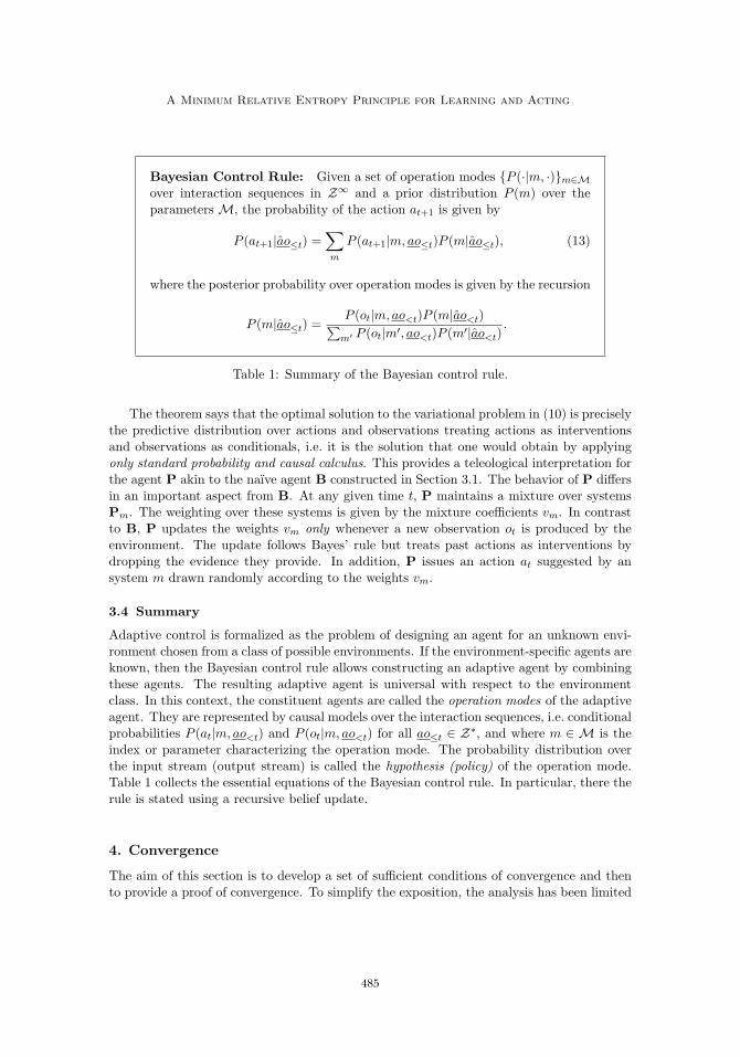
Bayesian Control Rule: Given a set of operation modes {P (·|m, ·)}m∈M

over interaction sequences in Z∞ and a prior distribution P (m) over theparameters M, the probability of the action at+1 is given by

P (at+1|ao≤t) =∑m

P (at+1|m, ao≤t)P (m|ao≤t), (13)

where the posterior probability over operation modes is given by the recursion

P (m|ao≤t) =P (ot|m, ao<t)P (m|ao<t)∑

m′ P (ot|m′, ao<t)P (m′|ao<t).

Table 1: Summary of the Bayesian control rule.

The theorem says that the optimal solution to the variational problem in (10) is preciselythe predictive distribution over actions and observations treating actions as interventionsand observations as conditionals, i.e. it is the solution that one would obtain by applyingonly standard probability and causal calculus. This provides a teleological interpretation forthe agent P akin to the naıve agent B constructed in Section 3.1. The behavior of P differsin an important aspect from B. At any given time t, P maintains a mixture over systemsPm. The weighting over these systems is given by the mixture coefficients vm. In contrastto B, P updates the weights vm only whenever a new observation ot is produced by theenvironment. The update follows Bayes’ rule but treats past actions as interventions bydropping the evidence they provide. In addition, P issues an action at suggested by ansystem m drawn randomly according to the weights vm.

3.4 Summary

Adaptive control is formalized as the problem of designing an agent for an unknown envi-ronment chosen from a class of possible environments. If the environment-specific agents areknown, then the Bayesian control rule allows constructing an adaptive agent by combiningthese agents. The resulting adaptive agent is universal with respect to the environmentclass. In this context, the constituent agents are called the operation modes of the adaptiveagent. They are represented by causal models over the interaction sequences, i.e. conditionalprobabilities P (at|m, ao<t) and P (ot|m, ao<t) for all ao≤t ∈ Z∗, and where m ∈ M is theindex or parameter characterizing the operation mode. The probability distribution overthe input stream (output stream) is called the hypothesis (policy) of the operation mode.Table 1 collects the essential equations of the Bayesian control rule. In particular, there therule is stated using a recursive belief update.

4. Convergence

The aim of this section is to develop a set of sufficient conditions of convergence and thento provide a proof of convergence. To simplify the exposition, the analysis has been limited

485

Ortega & Braun

to the case of controllers having a finite number of input-output models.

4.1 Policy Diagrams

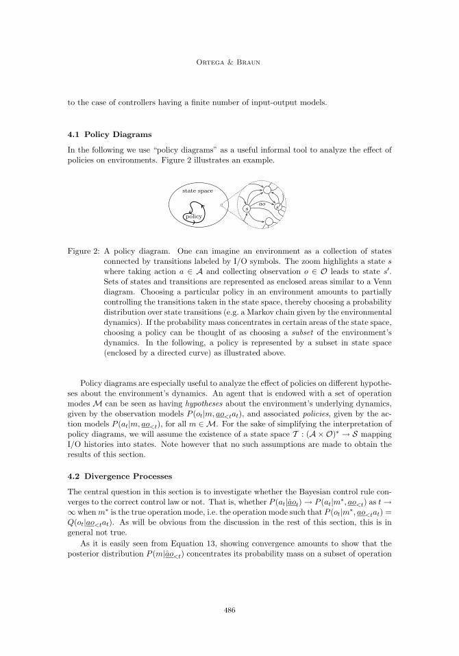
In the following we use “policy diagrams” as a useful informal tool to analyze the effect ofpolicies on environments. Figure 2 illustrates an example.

state space

policy

s s′ao

Figure 2: A policy diagram. One can imagine an environment as a collection of statesconnected by transitions labeled by I/O symbols. The zoom highlights a state swhere taking action a ∈ A and collecting observation o ∈ O leads to state s′.Sets of states and transitions are represented as enclosed areas similar to a Venndiagram. Choosing a particular policy in an environment amounts to partiallycontrolling the transitions taken in the state space, thereby choosing a probabilitydistribution over state transitions (e.g. a Markov chain given by the environmentaldynamics). If the probability mass concentrates in certain areas of the state space,choosing a policy can be thought of as choosing a subset of the environment’sdynamics. In the following, a policy is represented by a subset in state space(enclosed by a directed curve) as illustrated above.

Policy diagrams are especially useful to analyze the effect of policies on different hypothe-ses about the environment’s dynamics. An agent that is endowed with a set of operationmodes M can be seen as having hypotheses about the environment’s underlying dynamics,given by the observation models P (ot|m, ao<tat), and associated policies, given by the ac-tion models P (at|m, ao<t), for all m ∈ M. For the sake of simplifying the interpretation ofpolicy diagrams, we will assume the existence of a state space T : (A×O)∗ → S mappingI/O histories into states. Note however that no such assumptions are made to obtain theresults of this section.

4.2 Divergence Processes

The central question in this section is to investigate whether the Bayesian control rule con-verges to the correct control law or not. That is, whether P (at|aot) → P (at|m

∗, ao<t) as t →∞ when m∗ is the true operation mode, i.e. the operation mode such that P (ot|m

∗, ao<tat) =Q(ot|ao<tat). As will be obvious from the discussion in the rest of this section, this is ingeneral not true.

As it is easily seen from Equation 13, showing convergence amounts to show that theposterior distribution P (m|ao<t) concentrates its probability mass on a subset of operation

486


modes M∗ having essentially the same output stream as m∗,∑m∈M

P (at|m, ao<t)P (m|ao<t) ≈∑

m∈M∗

P (at|m∗, ao<t)P (m|ao<t) ≈ P (at|m

∗, ao<t).

Hence, understanding the asymptotic behavior of the posterior probabilities

P (m|ao≤t)

is crucial here. In particular, we need to understand under what conditions these quantitiesconverge to zero. The posterior can be rewritten as

P (m|ao≤t) =P (ao≤t|m)P (m)∑

m′∈M P (ao≤t|m′)P (m′)

=P (m)

∏tτ=1 P (oτ |m, ao<τaτ )∑

m′∈M P (m′)∏t

τ=1 P (oτ |m′, ao<τaτ ).

If all the summands but the one with index m∗ are dropped from the denominator, oneobtains the bound

P (m|ao≤t) ≤P (m)

P (m∗)

t∏τ=1

P (oτ |m, ao<τaτ )

P (oτ |m∗, ao<τaτ ),

which is valid for all m∗ ∈ M. From this inequality, it is seen that it is convenient toanalyze the behavior of the stochastic process

dt(m∗‖m) :=

t∑τ=1

lnP (oτ |m

∗, ao<τaτ )


which is the divergence process of m from the reference m∗. Indeed, if dt(m∗‖m) → ∞ as

t → ∞, then

limt→∞

P (m)

P (m∗)

t∏τ=1


P (oτ |m∗, ao<τaτ )= lim

t→∞

P (m)

P (m∗)· e−dt(m∗‖m) = 0,

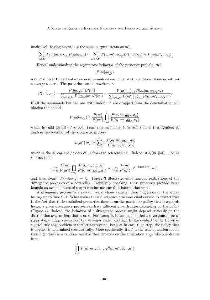
and thus clearly P (m|ao≤t) → 0. Figure 3 illustrates simultaneous realizations of thedivergence processes of a controller. Intuitively speaking, these processes provide lowerbounds on accumulators of surprise value measured in information units.

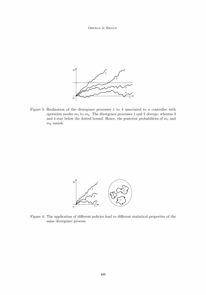
A divergence process is a random walk whose value at time t depends on the wholehistory up to time t−1. What makes these divergence processes cumbersome to characterizeis the fact that their statistical properties depend on the particular policy that is applied;hence, a given divergence process can have different growth rates depending on the policy(Figure 4). Indeed, the behavior of a divergence process might depend critically on thedistribution over actions that is used. For example, it can happen that a divergence processstays stable under one policy, but diverges under another. In the context of the Bayesiancontrol rule this problem is further aggravated, because in each time step, the policy thatis applied is determined stochastically. More specifically, if m∗ is the true operation mode,then dt(m

∗‖m) is a random variable that depends on the realization ao≤t which is drawnfrom

t∏τ=1

P (aτ |mτ , ao≤τ )P (oτ |m∗, ao≤τaτ ),

487

Ortega & Braun

0

1

2

3

4

t

dt

Figure 3: Realization of the divergence processes 1 to 4 associated to a controller withoperation modes m1 to m4. The divergence processes 1 and 2 diverge, whereas 3and 4 stay below the dotted bound. Hence, the posterior probabilities of m1 andm2 vanish.

0

1

1

2

2

3

3

t

dt

Figure 4: The application of different policies lead to different statistical properties of thesame divergence process.

488


where the m1, m2, . . . , mt are drawn themselves from P (m1), P (m2|ao1), . . . , P (mt|ao<t).To deal with the heterogeneous nature of divergence processes, one can introduce a

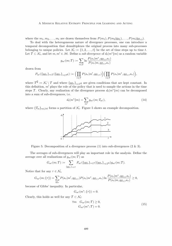
temporal decomposition that demultiplexes the original process into many sub-processesbelonging to unique policies. Let Nt := {1, 2, . . . , t} be the set of time steps up to time t.Let T ⊂ Nt, and let m, m′ ∈ M. Define a sub-divergence of dt(m

∗‖m) as a random variable

gm′(m; T ) :=∑τ∈T

lnP (oτ |m

∗, ao<τaτ )


drawn from

Pm′({aoτ}τ∈T |{aoτ}τ∈T � ) :=(∏

τ∈T

P (aτ |m′, ao<τ )

)(∏τ∈T

P (oτ |m∗, ao<τaτ )

),

where T � := Nt \ T and where {aoτ}τ∈T � are given conditions that are kept constant. Inthis definition, m′ plays the role of the policy that is used to sample the actions in the timesteps T . Clearly, any realization of the divergence process dt(m

∗‖m) can be decomposedinto a sum of sub-divergences, i.e.

dt(m∗‖m) =

∑m′

gm′(m; Tm′), (14)

where {Tm}m∈M forms a partition of Nt. Figure 5 shows an example decomposition.

0

1

2

3

t

dt

Figure 5: Decomposition of a divergence process (1) into sub-divergences (2 & 3).

The averages of sub-divergences will play an important role in the analysis. Define theaverage over all realizations of gm′(m; T ) as

Gm′(m; T ) :=∑

(aoτ)τ∈T

Pm′({aoτ}τ∈T |{aoτ}τ∈T � )gm′(m; T ).

Notice that for any τ ∈ Nt,

Gm′(m; {τ}) =∑ao

τ

P (aτ |m′, ao<τ )P (oτ |m

∗, ao<τaτ ) lnP (oτ |m

∗, ao<τaτ )

P (oτ |m, ao<τaτ )≥ 0,

because of Gibbs’ inequality. In particular,

Gm′(m∗; {τ}) = 0.

Clearly, this holds as well for any T ⊂ Nt:

∀m Gm′(m; T ) ≥ 0,

Gm′(m∗; T ) = 0.

(15)

489

Ortega & Braun

4.3 Boundedness

In general, a divergence process is very complex: virtually all the classes of distributionsthat are of interest in control go well beyond the assumptions of i.i.d. and stationarity. Thisincreased complexity can jeopardize the analytic tractability of the divergence process, suchthat no predictions about its asymptotic behavior can be made anymore. More specifically,if the growth rates of the divergence processes vary too much from realization to realiza-tion, then the posterior distribution over operation modes can vary qualitatively betweenrealizations. Hence, one needs to impose a stability requirement akin to ergodicity to limitthe class of possible divergence-processes to a class that is analytically tractable. For thispurpose the following property is introduced.

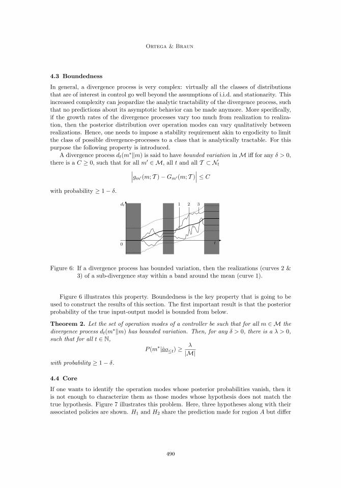
A divergence process dt(m∗‖m) is said to have bounded variation in M iff for any δ > 0,

there is a C ≥ 0, such that for all m′ ∈ M, all t and all T ⊂ Nt∣∣∣gm′(m; T ) − Gm′(m; T )∣∣∣ ≤ C

with probability ≥ 1 − δ.

0

1 2 3

t

dt

Figure 6: If a divergence process has bounded variation, then the realizations (curves 2 &3) of a sub-divergence stay within a band around the mean (curve 1).

Figure 6 illustrates this property. Boundedness is the key property that is going to beused to construct the results of this section. The first important result is that the posteriorprobability of the true input-output model is bounded from below.

Theorem 2. Let the set of operation modes of a controller be such that for all m ∈ M thedivergence process dt(m

∗‖m) has bounded variation. Then, for any δ > 0, there is a λ > 0,such that for all t ∈ N,

P (m∗|ao≤t) ≥λ

|M|

with probability ≥ 1 − δ.

4.4 Core

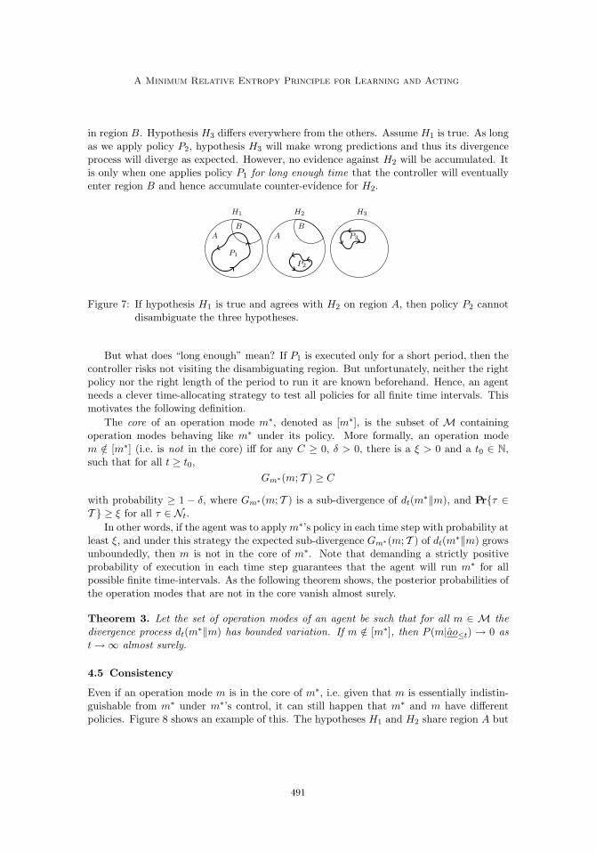
If one wants to identify the operation modes whose posterior probabilities vanish, then itis not enough to characterize them as those modes whose hypothesis does not match thetrue hypothesis. Figure 7 illustrates this problem. Here, three hypotheses along with theirassociated policies are shown. H1 and H2 share the prediction made for region A but differ

490


in region B. Hypothesis H3 differs everywhere from the others. Assume H1 is true. As longas we apply policy P2, hypothesis H3 will make wrong predictions and thus its divergenceprocess will diverge as expected. However, no evidence against H2 will be accumulated. Itis only when one applies policy P1 for long enough time that the controller will eventuallyenter region B and hence accumulate counter-evidence for H2.

H1

P1

H2

P2

H3

P3A A

B B

Figure 7: If hypothesis H1 is true and agrees with H2 on region A, then policy P2 cannotdisambiguate the three hypotheses.

But what does “long enough” mean? If P1 is executed only for a short period, then thecontroller risks not visiting the disambiguating region. But unfortunately, neither the rightpolicy nor the right length of the period to run it are known beforehand. Hence, an agentneeds a clever time-allocating strategy to test all policies for all finite time intervals. Thismotivates the following definition.

The core of an operation mode m∗, denoted as [m∗], is the subset of M containingoperation modes behaving like m∗ under its policy. More formally, an operation modem /∈ [m∗] (i.e. is not in the core) iff for any C ≥ 0, δ > 0, there is a ξ > 0 and a t0 ∈ N,such that for all t ≥ t0,

Gm∗(m; T ) ≥ C

with probability ≥ 1 − δ, where Gm∗(m; T ) is a sub-divergence of dt(m∗‖m), and Pr{τ ∈

T } ≥ ξ for all τ ∈ Nt.

In other words, if the agent was to apply m∗’s policy in each time step with probability atleast ξ, and under this strategy the expected sub-divergence Gm∗(m; T ) of dt(m

∗‖m) growsunboundedly, then m is not in the core of m∗. Note that demanding a strictly positiveprobability of execution in each time step guarantees that the agent will run m∗ for allpossible finite time-intervals. As the following theorem shows, the posterior probabilities ofthe operation modes that are not in the core vanish almost surely.

Theorem 3. Let the set of operation modes of an agent be such that for all m ∈ M thedivergence process dt(m

∗‖m) has bounded variation. If m /∈ [m∗], then P (m|ao≤t) → 0 ast → ∞ almost surely.

4.5 Consistency

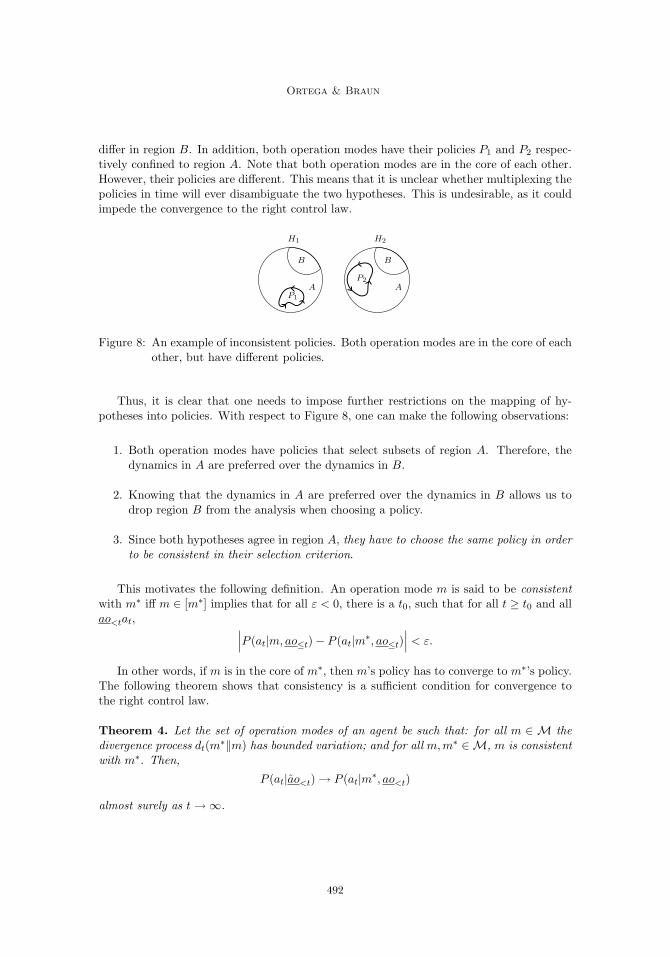
Even if an operation mode m is in the core of m∗, i.e. given that m is essentially indistin-guishable from m∗ under m∗’s control, it can still happen that m∗ and m have differentpolicies. Figure 8 shows an example of this. The hypotheses H1 and H2 share region A but

491

Ortega & Braun

differ in region B. In addition, both operation modes have their policies P1 and P2 respec-tively confined to region A. Note that both operation modes are in the core of each other.However, their policies are different. This means that it is unclear whether multiplexing thepolicies in time will ever disambiguate the two hypotheses. This is undesirable, as it couldimpede the convergence to the right control law.

H1

P1

H2

P2

A A

B B

Figure 8: An example of inconsistent policies. Both operation modes are in the core of eachother, but have different policies.

Thus, it is clear that one needs to impose further restrictions on the mapping of hy-potheses into policies. With respect to Figure 8, one can make the following observations:

1. Both operation modes have policies that select subsets of region A. Therefore, thedynamics in A are preferred over the dynamics in B.

2. Knowing that the dynamics in A are preferred over the dynamics in B allows us todrop region B from the analysis when choosing a policy.

3. Since both hypotheses agree in region A, they have to choose the same policy in orderto be consistent in their selection criterion.

This motivates the following definition. An operation mode m is said to be consistentwith m∗ iff m ∈ [m∗] implies that for all ε < 0, there is a t0, such that for all t ≥ t0 and allao<tat, ∣∣∣P (at|m, ao≤t) − P (at|m

∗, ao≤t)∣∣∣ < ε.

In other words, if m is in the core of m∗, then m’s policy has to converge to m∗’s policy.The following theorem shows that consistency is a sufficient condition for convergence tothe right control law.

Theorem 4. Let the set of operation modes of an agent be such that: for all m ∈ M thedivergence process dt(m

∗‖m) has bounded variation; and for all m, m∗ ∈ M, m is consistentwith m∗. Then,

P (at|ao<t) → P (at|m∗, ao<t)

almost surely as t → ∞.

492


4.6 Summary

In this section, a proof of convergence of the Bayesian control rule to the true operationmode has been provided for a finite set of operation modes. For this convergence result tohold, two necessary conditions are assumed: boundedness and consistency. The first one,boundedness, imposes the stability of divergence processes under the partial influence of thepolicies contained within the set of operation modes. This condition can be regarded asan ergodicity assumption. The second one, consistency, requires that if a hypothesis makesthe same predictions as another hypothesis within its most relevant subset of dynamics,then both hypotheses share the same policy. This relevance is formalized as the core of anoperation mode. The concepts and proof strategies strengthen the intuition about potentialpitfalls that arise in the context of controller design. In particular we could show thatthe asymptotic analysis can be recast as the study of concurrent divergence processes thatdetermine the evolution of the posterior probabilities over operation modes, thus abstractingaway from the details of the classes of I/O distributions. The extension of these results toinfinite sets of operation modes is left for future work. For example, one could thinkof partitioning a continuous space of operation modes into “essentially different” regionswhere representative operation modes subsume their neighborhoods (Grunwald, 2007).

5. Examples

In this section we illustrate the usage of the Bayesian control rule on two examples thatare very common in the reinforcement learning literature: multi-armed bandits and Markovdecision processes.

5.1 Bandit Problems

Consider the multi-armed bandit problem (Robbins, 1952). The problem is stated as follows.Suppose there is an N -armed bandit, i.e. a slot-machine with N levers. When pulled, leveri provides a reward drawn from a Bernoulli distribution with a bias hi specific to that lever.That is, a reward r = 1 is obtained with probability hi and a reward r = 0 with probability1−hi. The objective of the game is to maximize the time-averaged reward through iterativepulls. There is a continuum range of stationary strategies, each one parameterized by Nprobabilities {si}

Ni=1 indicating the probabilities of pulling each lever. The difficulty arising

in the bandit problem is to balance reward maximization based on the knowledge alreadyacquired with attempting new actions to further improve knowledge. This dilemma is knownas the exploration versus exploitation tradeoff (Sutton & Barto, 1998).

This is an ideal task for the Bayesian control rule, because each possible bandit has aknown optimal agent. Indeed, a bandit can be represented by an N -dimensional bias vectorm = [m1, . . . , mN ] ∈ M = [0; 1]N . Given such a bandit, the optimal policy consists inpulling the lever with the highest bias. That is, an operation mode is given by:

hi = P (ot = 1|m, at = i) = mi si = P (at = i|m) =

{1 if i = maxj{mj},

0 else.

493

Ortega & Braun

0 10

1

0

1

01

1

a)

m1

m2

m1 ≥ m2

b)

m1

m2

m3

m2 ≥ m1, m3

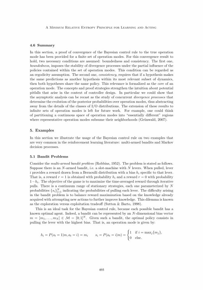
Figure 9: The space of bandit configurations can be partitioned into N regions accordingto the optimal lever. Panel a and b show the 2-armed and 3-armed bandit casesrespectively.

To apply the Bayesian control rule, it is necessary to fix a prior distribution over thebandit configurations. Assuming a uniform distribution, the Bayesian control rule is

P (at+1 = i|ao≤t) =

∫M

P (at+1 = i|m)P (m|ao≤t) (16)

with the update rule given by

P (m|ao≤t) =P (m)

∏tτ=1 P (oτ |m, aτ )∫

MP (m′)

∏tτ=1 P (oτ |m′, aτ ) dm′

=N∏

j=1

mrj

j (1 − mj)fj

B(rj + 1, fj + 1)(17)

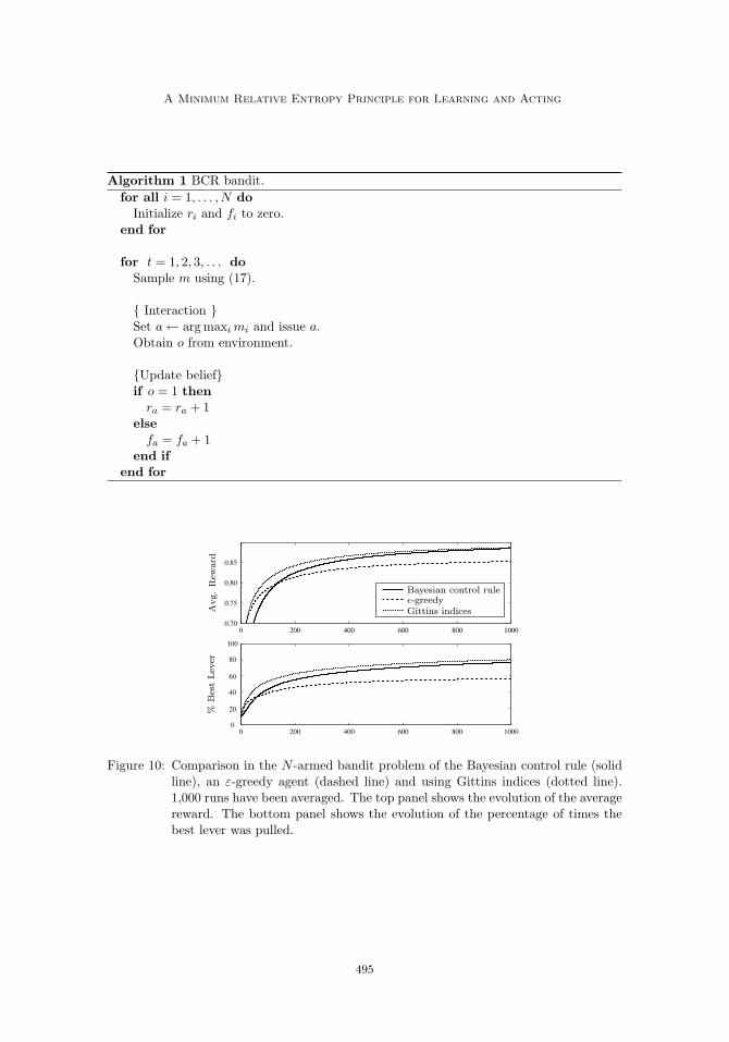
where rj and fj are the counts of the number of times a reward has been obtained frompulling lever j and the number of times no reward was obtained respectively. Observe thathere the summation over discrete operation modes has been replaced by an integral overthe continuous space of configurations. In the last expression we see that the posteriordistribution over the lever biases is given by a product of N Beta distributions. Thus,sampling an action amounts to first sample an operation mode m by obtaining each biasmi from a Beta distribution with parameters ri + 1 and fi + 1, and then choosing theaction corresponding to the highest bias a = arg maxi mi. The pseudo-code can be seen inAlgorithm 1.

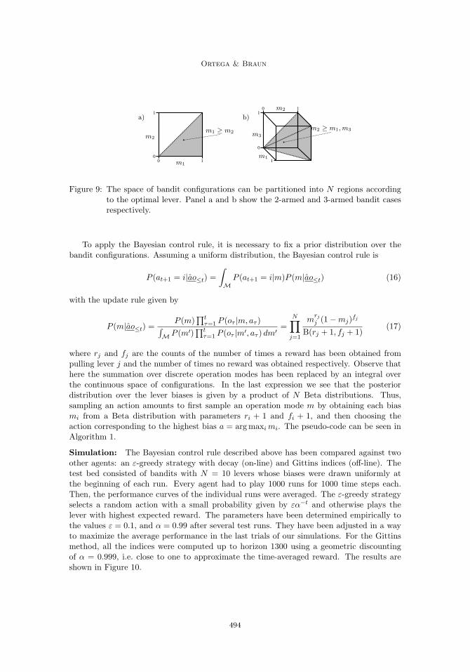
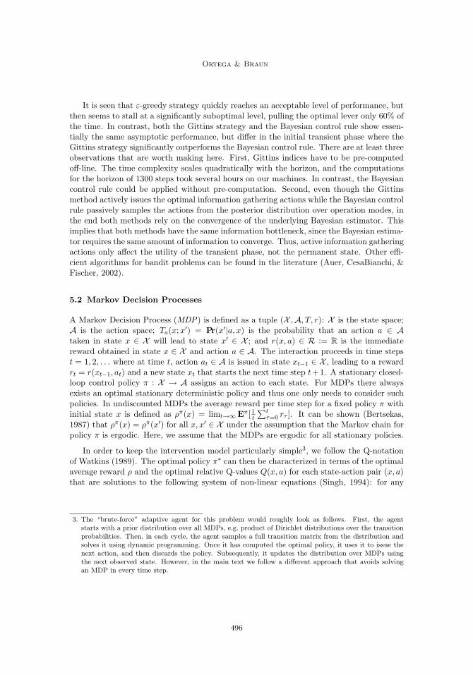
Simulation: The Bayesian control rule described above has been compared against twoother agents: an ε-greedy strategy with decay (on-line) and Gittins indices (off-line). Thetest bed consisted of bandits with N = 10 levers whose biases were drawn uniformly atthe beginning of each run. Every agent had to play 1000 runs for 1000 time steps each.Then, the performance curves of the individual runs were averaged. The ε-greedy strategyselects a random action with a small probability given by εα−t and otherwise plays thelever with highest expected reward. The parameters have been determined empirically tothe values ε = 0.1, and α = 0.99 after several test runs. They have been adjusted in a wayto maximize the average performance in the last trials of our simulations. For the Gittinsmethod, all the indices were computed up to horizon 1300 using a geometric discountingof α = 0.999, i.e. close to one to approximate the time-averaged reward. The results areshown in Figure 10.

494


Algorithm 1 BCR bandit.

for all i = 1, . . . , N doInitialize ri and fi to zero.

end for

for t = 1, 2, 3, . . . doSample m using (17).

{ Interaction }Set a ← arg maxi mi and issue a.Obtain o from environment.

{Update belief}if o = 1 then

ra = ra + 1else

fa = fa + 1end if

end for

200 400 600 800 100000.70

0.75

0.80

0.85

200 400 600 800 100000

20

40

60

80

100

Avg.

Rew

ard

%B

est

Lev

er

Bayesian control ruleε-greedyGittins indices

Figure 10: Comparison in the N -armed bandit problem of the Bayesian control rule (solidline), an ε-greedy agent (dashed line) and using Gittins indices (dotted line).1,000 runs have been averaged. The top panel shows the evolution of the averagereward. The bottom panel shows the evolution of the percentage of times thebest lever was pulled.

495

Ortega & Braun

It is seen that ε-greedy strategy quickly reaches an acceptable level of performance, butthen seems to stall at a significantly suboptimal level, pulling the optimal lever only 60% ofthe time. In contrast, both the Gittins strategy and the Bayesian control rule show essen-tially the same asymptotic performance, but differ in the initial transient phase where theGittins strategy significantly outperforms the Bayesian control rule. There are at least threeobservations that are worth making here. First, Gittins indices have to be pre-computedoff-line. The time complexity scales quadratically with the horizon, and the computationsfor the horizon of 1300 steps took several hours on our machines. In contrast, the Bayesiancontrol rule could be applied without pre-computation. Second, even though the Gittinsmethod actively issues the optimal information gathering actions while the Bayesian controlrule passively samples the actions from the posterior distribution over operation modes, inthe end both methods rely on the convergence of the underlying Bayesian estimator. Thisimplies that both methods have the same information bottleneck, since the Bayesian estima-tor requires the same amount of information to converge. Thus, active information gatheringactions only affect the utility of the transient phase, not the permanent state. Other effi-cient algorithms for bandit problems can be found in the literature (Auer, CesaBianchi, &Fischer, 2002).

5.2 Markov Decision Processes

A Markov Decision Process (MDP) is defined as a tuple (X ,A, T, r): X is the state space;A is the action space; Ta(x;x′) = Pr(x′|a, x) is the probability that an action a ∈ Ataken in state x ∈ X will lead to state x′ ∈ X ; and r(x, a) ∈ R := R is the immediatereward obtained in state x ∈ X and action a ∈ A. The interaction proceeds in time stepst = 1, 2, . . . where at time t, action at ∈ A is issued in state xt−1 ∈ X , leading to a rewardrt = r(xt−1, at) and a new state xt that starts the next time step t+1. A stationary closed-loop control policy π : X → A assigns an action to each state. For MDPs there alwaysexists an optimal stationary deterministic policy and thus one only needs to consider suchpolicies. In undiscounted MDPs the average reward per time step for a fixed policy π withinitial state x is defined as ρπ(x) = limt→∞ Eπ[1

t

∑tτ=0 rτ ]. It can be shown (Bertsekas,

1987) that ρπ(x) = ρπ(x′) for all x, x′ ∈ X under the assumption that the Markov chain forpolicy π is ergodic. Here, we assume that the MDPs are ergodic for all stationary policies.

In order to keep the intervention model particularly simple3, we follow the Q-notationof Watkins (1989). The optimal policy π∗ can then be characterized in terms of the optimalaverage reward ρ and the optimal relative Q-values Q(x, a) for each state-action pair (x, a)that are solutions to the following system of non-linear equations (Singh, 1994): for any

3. The “brute-force” adaptive agent for this problem would roughly look as follows. First, the agentstarts with a prior distribution over all MDPs, e.g. product of Dirichlet distributions over the transitionprobabilities. Then, in each cycle, the agent samples a full transition matrix from the distribution andsolves it using dynamic programming. Once it has computed the optimal policy, it uses it to issue thenext action, and then discards the policy. Subsequently, it updates the distribution over MDPs usingthe next observed state. However, in the main text we follow a different approach that avoids solvingan MDP in every time step.

496


state x ∈ X and action a ∈ A,

Q(x, a) + ρ = r(x, a) +∑x′∈X

Pr(x′|x, a)[max

a′Q(x′, a′)

]= r(x, a) + Ex′

[max

a′Q(x′, a′)

∣∣∣x, a].

(18)

The optimal policy can then be defined as π∗(x) := arg maxa Q(x, a) for any state x ∈ X .Again this setup allows for a straightforward solution with the Bayesian control rule,

because each learnable MDP (characterized by the Q-values and the average reward) hasa known solution π∗. Accordingly, an operation mode m is given by m = [Q, ρ] ∈ M =R|A|×|O|+1. To obtain a likelihood model for inference over m, we realize that Equation 18can be rewritten such that it predicts the instantaneous reward r(x, a) as the sum of a meaninstantaneous reward ξm plus a noise term ν given the Q-values and the average reward ρfor the MDP labeled by m

r(x, a) = Q(x, a) + ρ − maxa′

Q(x′, a′)︸︷︷︸mean instantaneous reward ξm(x,a,x′)

+ maxa′

Q(x′, a′) − E[maxa′

Q(x′, a′)|x, a]︸︷︷︸noise ν

Assuming that ν can be reasonably approximated by a normal distribution N(0, 1/p) withprecision p, we can write down a likelihood model for the immediate reward r using theQ-values and the average reward, i.e.

P (r|m, x, a, x′) =

√p

2πexp

{−

p

2(r − ξm(x, a, x′))2

}. (19)

In order to determine the intervention model for each operation mode, we can simply exploitthe above properties of the Q-values, which gives

P (a|m, x) =

{1 if a = arg maxa′ Q(x, a′)

0 else.(20)

To apply the Bayesian control rule, the posterior distribution P (m|a≤t, x≤t) needs to becomputed. Fortunately, due to the simplicity of the likelihood model, one can easily devise aconjugate prior distribution and apply standard inference methods (see Appendix A.5). Ac-tions are again determined by sampling operation modes from this posterior and executingthe action suggested by the corresponding intervention models. The resulting algorithm isvery similar to Bayesian Q-learning (Dearden, Friedman, & Russell, 1998; Dearden, Fried-man, & Andre, 1999), but differs in the way actions are selected. The pseudo-code is listedin Algorithm 2.

Simulation: We have tested our MDP-agent in a grid-world example. To give an intuitionof the achieved performance, the results are contrasted with those achieved by R-learning.We have used the R-learning variant presented in the work of Singh (1994, Algorithm 3)together with the uncertainty exploration strategy (Mahadevan, 1996). The correspondingupdate equations are

Q(x, a) ← (1 − α)Q(x, a) + α(r − ρ + max

a′Q(x′, a′)

)ρ ← (1 − β)ρ + β

(r + max

a′Q(x′, a′) − Q(x, a)

),

(21)

497

Ortega & Braun

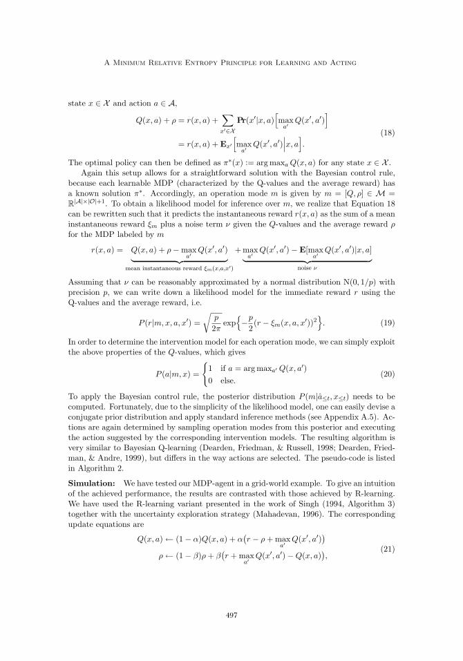
Algorithm 2 BCR-MDP Gibbs sampler.

Initialize entries of λ and μ to zero.Set initial state to x ← x0.for t = 1, 2, 3, . . . do

{Gibbs sweep}Sample ρ using (30).for all Q(y, b) of visited states do

Sample Q(y, b) using (31).end for

{ Interaction }Set a ← arg maxa′ Q(x, a′) and issue a.Obtain o = (r, x′) from environment.

{Update hyperparameters}

μ(x, a, x′) ← λ(x,a,x′)μ(x,a,x′)+p r

λ(x,a,x′)+p

λ(x, a, x′) ← λ(x, a, x′) + p

Set x ← x′.end for

1250 250 375500

x1000 time steps

0.0

0.1

0.2

0.3

0.4f) Average Reward

C=30

Bayesian control rule

c) R-learning, C=5 d) R-learning, C=30b) Bayesian control rule

init

ial

5,0

00

ste

ps

last

5,0

00

ste

ps

a) 7x7 Maze

goal

membranes

highprobability

lowprobability

C=5

C=200

e) R-learning, C=200

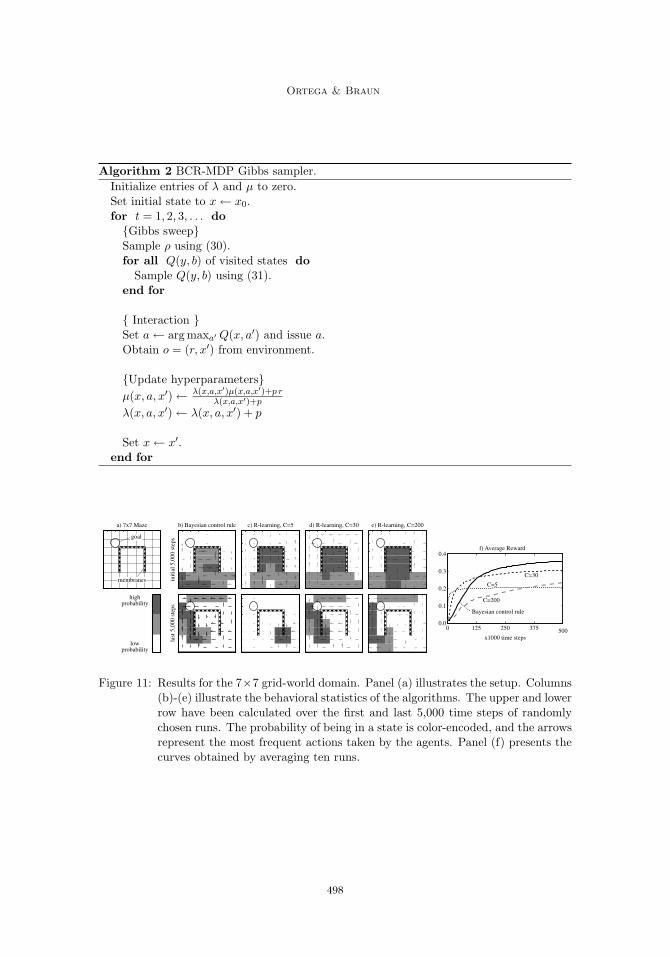
Figure 11: Results for the 7×7 grid-world domain. Panel (a) illustrates the setup. Columns(b)-(e) illustrate the behavioral statistics of the algorithms. The upper and lowerrow have been calculated over the first and last 5,000 time steps of randomlychosen runs. The probability of being in a state is color-encoded, and the arrowsrepresent the most frequent actions taken by the agents. Panel (f) presents thecurves obtained by averaging ten runs.

498


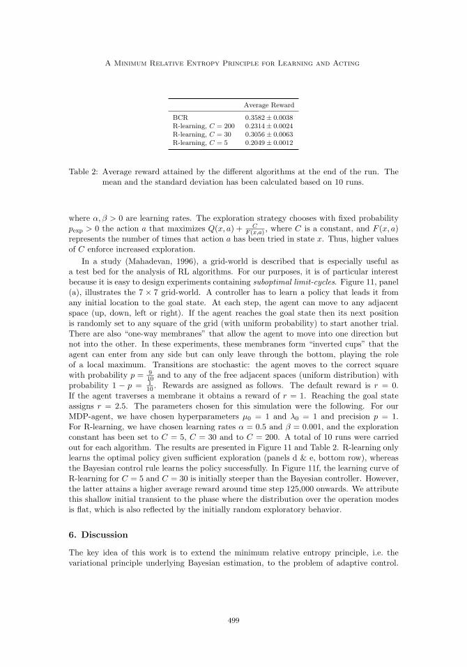
Average Reward

BCR 0.3582± 0.0038R-learning, C = 200 0.2314± 0.0024R-learning, C = 30 0.3056± 0.0063R-learning, C = 5 0.2049± 0.0012

Table 2: Average reward attained by the different algorithms at the end of the run. Themean and the standard deviation has been calculated based on 10 runs.

where α, β > 0 are learning rates. The exploration strategy chooses with fixed probabilitypexp > 0 the action a that maximizes Q(x, a) + C

F (x,a) , where C is a constant, and F (x, a)represents the number of times that action a has been tried in state x. Thus, higher valuesof C enforce increased exploration.

In a study (Mahadevan, 1996), a grid-world is described that is especially useful asa test bed for the analysis of RL algorithms. For our purposes, it is of particular interestbecause it is easy to design experiments containing suboptimal limit-cycles. Figure 11, panel(a), illustrates the 7 × 7 grid-world. A controller has to learn a policy that leads it fromany initial location to the goal state. At each step, the agent can move to any adjacentspace (up, down, left or right). If the agent reaches the goal state then its next positionis randomly set to any square of the grid (with uniform probability) to start another trial.There are also “one-way membranes” that allow the agent to move into one direction butnot into the other. In these experiments, these membranes form “inverted cups” that theagent can enter from any side but can only leave through the bottom, playing the roleof a local maximum. Transitions are stochastic: the agent moves to the correct squarewith probability p = 9

10 and to any of the free adjacent spaces (uniform distribution) withprobability 1 − p = 1

10 . Rewards are assigned as follows. The default reward is r = 0.If the agent traverses a membrane it obtains a reward of r = 1. Reaching the goal stateassigns r = 2.5. The parameters chosen for this simulation were the following. For ourMDP-agent, we have chosen hyperparameters μ0 = 1 and λ0 = 1 and precision p = 1.For R-learning, we have chosen learning rates α = 0.5 and β = 0.001, and the explorationconstant has been set to C = 5, C = 30 and to C = 200. A total of 10 runs were carriedout for each algorithm. The results are presented in Figure 11 and Table 2. R-learning onlylearns the optimal policy given sufficient exploration (panels d & e, bottom row), whereasthe Bayesian control rule learns the policy successfully. In Figure 11f, the learning curve ofR-learning for C = 5 and C = 30 is initially steeper than the Bayesian controller. However,the latter attains a higher average reward around time step 125,000 onwards. We attributethis shallow initial transient to the phase where the distribution over the operation modesis flat, which is also reflected by the initially random exploratory behavior.

6. Discussion

The key idea of this work is to extend the minimum relative entropy principle, i.e. thevariational principle underlying Bayesian estimation, to the problem of adaptive control.

499

Ortega & Braun

From a coding point of view, this work extends the idea of maximal compression of theobservation stream to the whole experience of the agent containing both the agent’s actionsand observations. This not only minimizes the amount of bits to write when saving/encodingthe I/O stream, but it also minimizes the amount of bits required to produce/decode anaction (MacKay, 2003, Ch. 6).

This extension is non-trivial, because there is an important caveat for coding I/O se-quences: unlike observations, actions do not carry any information that could be used forinference in adaptive coding because actions are issued by the decoder itself. The problemis that doing inference on ones own actions is logically inconsistent and leads to paradoxes(Nozick, 1969). This seemingly innocuous issue has turned out to be very intricate andhas been investigated intensely in the recent past by researchers focusing on the issue ofcausality (Pearl, 2000; Spirtes et al., 2000; Dawid, 2010). Our work contributes to this bodyof research by providing further evidence that actions cannot be treated using probabilitycalculus alone.

If the causal dependencies are carefully taken into account, then minimizing the relativeentropy leads to a rule for adaptive control which we called the Bayesian control rule. Thisrule allows combining a class of task-specific agents into an agent that is universal withrespect to this class. The resulting control law is a simple stochastic control rule that iscompletely general and parameter-free. As the analysis in this paper shows, this controlrule converges to the true control law under mild assumptions.

6.1 Critical Issues

• Causality. Virtually every adaptive control method in the literature successfully treatsactions as conditionals over observation streams and never worries about causality.Thus, why bother about interventions? In a decision-theoretic setup, the decisionmaker chooses a policy π∗ ∈ Π maximizing the expected utility U over the outcomesω ∈ Ω, i.e. π∗ := arg maxπ E[U |π] =

∑ω Pr(ω|π)U(ω). “Choosing π∗” is formally

equivalent to choosing the Kronecker delta function δππ∗ as the probability distribution

over policies. In this case, the conditional probabilities Pr(ω|π) and Pr(ω|π) coincide,since

Pr(ω, π) = Pr(π)Pr(ω|π) = δππ∗Pr(ω|π) = Pr(ω, π).

In this sense, the choice of the policy causally precedes the interactions. As we havediscussed in Section 3 however, when there is uncertainty about the policy (i.e. Pr(π) �=δππ∗), then causal belief updates are crucial. Essentially, this problem arises because

the uncertainty over the policy is resolved during the interactions. Hence, treatingactions as interventions seamlessly extends them to the status of random variables.

• Where do prior probabilities/likelihood models/policies come from? The predictor inthe Bayesian control rule is essentially a Bayesian predictor and thereby entails (al-most) the same modeling paradigm. The designer has to define a class of hypothesesover the environments, construct appropriate likelihood models, and choose a suitableprior probability distribution to capture the model’s uncertainty. Similarly, under suf-ficient domain knowledge, an analogous procedure can be applied to construct suitableoperation modes. However, there are many situations where this is a difficult or even

500


intractable problem in itself. For example, one can design a class of operation modesby pre-computing the optimal policies for a given class of environments. Formally, letΘ be a class of hypotheses modeling environments and let Π be class of policies. Givena utility criterion U , define the set of operation modes M := {mθ}θ∈Θ by construct-ing each operation mode as mθ := (θ, π∗), π∗ ∈ π, where π∗ := arg maxπ E[U |θ, π].However, computing the optimal policy π∗ is in many cases intractable. In somecases, this can be remedied by characterizing the operation modes through optimalityequations which are solved by probabilistic inference as in the example of the MDPagent in Section 5.2. Recently, we have applied a similar approach to adaptive controlproblems with linear quadratic regulators (Braun & Ortega, 2010).

• Problems of Bayesian methods. The Bayesian control rule treats an adaptive controlproblem as a Bayesian inference problem. Hence, all the problems typically associatedwith Bayesian methods carry over to agents constructed with the Bayesian controlrule. These problems are of both analytical and computational nature. For example,there are many probabilistic models where the posterior distribution does not have aclosed-form solution. Also, exact probabilistic inference is in general computationallyvery intensive. Even though there is a large literature in efficient/approximate infer-ence algorithms for particular problem classes (Bishop, 2006), not many of them aresuitable for on-line probabilistic inference in more realistic environment classes.

• Bayesian control rule versus Bayes-optimal control. Directly maximizing the (sub-jective) expected utility for a given environment class is not the same as minimizingthe expected relative entropy for a given class of operation modes. The two methodsare based on different assumptions and optimality principles. As such, the Bayesiancontrol rule is not a Bayes-optimal controller. Indeed, it is easy to design experimentswhere the Bayesian control rule converges exponentially slower (or does not convergeat all) than a Bayes-optimal controller to the maximum utility. Consider the followingsimple example: Environment 1 is a k-state MDP in which only k consecutive actionsA reach a state with reward +1. Any interception with a B-action leads back to theinitial state. Consider a second environment which is like the first but actions A andB are interchanged. A Bayes-optimal controller figures out the true environment in kactions (either k consecutive A’s or B’s). Consider now the Bayesian control rule: Theoptimal action in Environment 1 is A, in Environment 2 is B. A uniform (1

2 , 12) prior

over the operation modes stays a uniform posterior as long as no reward has beenobserved. Hence the Bayesian control rule chooses at each time-step A and B withequal probability. With this policy it takes about 2k actions to accidentally choose arow of A’s (or B’s) of length k. From then on the Bayesian control rule is optimaltoo. So a Bayes-optimal controller converges in time k, while the Bayesian controlrule needs exponentially longer. One way to remedy this problem might be to allowthe Bayesian control rule to sample actions from the same operation mode for severaltime steps in a row rather than randomizing controllers in every cycle. However, ifone considers non-stationary environments this strategy can also break down. Con-sider, for example, an increasing MDP with k =

⌈10√

t⌉, in which a Bayes-optimal

controller converges in 100 steps, while the Bayesian control rule does not convergeat all in most realizations, because the boundedness assumption is violated.

501

Ortega & Braun

6.2 Relation to Existing Approaches

Some of the ideas underlying this work are not unique to the Bayesian control rule. Thefollowing is a selection of previously published work in the recent Bayesian reinforcementlearning literature where related ideas can be found.

• Compression principles. In the literature, there is an important amount of workrelating compression to intelligence (MacKay, 2003; Hutter, 2004b). In particular, ithas been even proposed that compression ratio is an objective quantitative measure ofintelligence (Mahoney, 1999). Compression has also been used as a basis for a theoryof curiosity, creativity and beauty (Schmidhuber, 2009).

• Mixture of experts. Passive sequence prediction by mixing experts has been studiedextensively in the literature (Cesa-Bianchi & Lugosi, 2006). In a study on online-predictors (Hutter, 2004a), Bayes-optimal predictors are mixed. Bayes-mixtures canalso be used for universal prediction (Hutter, 2003). For the control case, the ideaof using mixtures of expert-controllers has been previously evoked in models like theMOSAIC-architecture (Haruno, Wolpert, & Kawato, 2001). Universal learning withBayes mixtures of experts in reactive environments has been studied in the work ofPoland and Hutter (2005) and Hutter (2002).

• Stochastic action selection. The idea of using actions as random variables, and theproblems that this entails, has been expressed in the work of Hutter (2004b, Problem5.1). The study in Section 3 can be regarded as a thorough investigation of this openproblem. Other stochastic action selection approaches are found in the thesis of Wy-att (1997) who examines exploration strategies for (PO)MDPs, in learning automata(Narendra & Thathachar, 1974) and in probability matching (Duda, Hart, & Stork,2001) amongst others. In particular, the thesis discusses theoretical properties ofan extension to probability matching in the context of multi-armed bandit problems.There, it is proposed to choose a lever according to how likely it is to be optimal andit is shown that this strategy converges, thus providing a simple method for guidingexploration.

• Relative entropy criterion. The usage of a minimum relative entropy criterion toderive control laws underlies the KL-control methods developed in the work of Todorov(2006, 2009) and Kappen et al. (2010). There, it has been shown that a large classof optimal control problems can be solved very efficiently if the problem statementis reformulated as the minimization of the deviation of the dynamics of a controlledsystem from the uncontrolled system. A related idea is to conceptualize planning asan inference problem (Toussaint, Harmeling, & Storkey, 2006). This approach is basedon an equivalence between maximization of the expected future return and likelihoodmaximization which is both applicable to MDPs and POMDPs. Algorithms based onthis duality have become an active field of current research. See for example the workof Rasmussen and Deisenroth (2008), where very fast model-based RL techniques areused for control in continuous state and action spaces.

502


7. Conclusions

This work introduces the Bayesian control rule, a Bayesian rule for adaptive control. Thekey feature of this rule is the special treatment of actions based on causal calculus and thedecomposition of an adaptive agent into a mixture of operation modes, i.e. environment-specific agents. The rule is derived by minimizing the expected relative entropy from thetrue operation mode and by carefully distinguishing between actions and observations. Fur-thermore, the Bayesian control rule turns out to be exactly the predictive distribution overthe next action given the past interactions that one would obtain by using only probabilityand causal calculus. Furthermore, it is shown that agents constructed with the Bayesiancontrol rule converge to the true operation mode under mild assumptions: boundedness,which is related to ergodicity; and consistency, demanding that two indistinguishable hy-potheses share the same policy.

We have presented the Bayesian control rule as a way to solve adaptive control problemsbased on a minimum relative entropy principle. Thus, the Bayesian control rule can eitherbe regarded as a new principled approach to adaptive control under a novel optimalitycriterion or as a heuristic approximation to traditional Bayes-optimal control. Since ittakes on a similar form to Bayes’ rule, the adaptive control problem could then be translatedinto an on-line inference problem where actions are sampled stochastically from a posteriordistribution. It is important to note, however, that the problem statement as formulatedhere and the usual Bayes-optimal approach in adaptive control are not the same. In thefuture the relationship between these two problem statements deserves further investigation.

Acknowledgments

We thank Marcus Hutter, David Wingate, Zoubin Ghahramani, Jose Aliste, Jose Donoso,Humberto Maturana and the anonymous reviewers for comments on earlier versions of thismanuscript and/or inspiring discussions. We thank the Ministerio de Planificacion de Chile(MIDEPLAN) and the Bohringer-Ingelheim-Fonds (BIF) for funding.

Appendix A. Proofs

A.1 Proof of Theorem 1

Proof. The proof follows the same line of argument as the solution to Equation 3 withthe crucial difference that actions are treated as interventions. Consider without loss ofgenerality the summand

∑m P (m)Cat

m in Equation 9. Note that the relative entropy can bewritten as a difference of two logarithms, where only one term depends on Pr to be varied.Therefore, one can pull out the other term and write it as a constant c. This yields

c −∑m

P (m)∑ao

<t

P (ao<t|m)∑at

P (at|m, ao<t) lnPr(at|ao<t).

503

Ortega & Braun

Substituting P (ao<t|m) by P (m|ao<t)P (ao<t)/P (m) using Bayes’ rule and further rear-rangement of the terms leads to

= c −∑m

∑ao

<t

P (m|ao<t)P (ao<t)∑at

P (at|m, ao<t) lnPr(at|ao<t)

= c −∑ao

<t

P (ao<t)∑at

P (at|ao<t) lnPr(at|ao<t).

The inner sum has the form −∑

x p(x) ln q(x), i.e. the cross-entropy between q(x) and p(x),which is minimized when q(x) = p(x) for all x. Let P denote the optimum distributionfor Pr. By choosing this optimum one obtains P(at|ao<t) = P (at|ao<t) for all at. Note thatthe solution to this variational problem is independent of the weighting P (ao<t). Since thesame argument applies to any summand

∑m P (m)Caτ

m and∑

m P (m)Coτ

m in Equation 9,their variational problems are mutually independent. Hence,

P(at|ao<t) = P (at|ao<t) P(ot|ao<t) = P (ot|ao<tat)

for all ao≤t ∈ Z∗. For P (at|ao<t), introduce the variable m via a marginalization and thenapply the chain rule:

P (at|ao<t) =∑m

P (at+1|m, ao<t)P (m|ao<t).

The term P (m|ao≤t) can be further developed as

P (m|ao<t) =P (ao<t|m)P (m)∑

m′ P (ao<t|m′)P (m′)

=P (m)

∏t−1τ=1 P (aτ |m, ao<τ )P (oτ |m, ao<τ aτ )∑

m′ P (m′)∏t−1

τ=1 P (aτ |m′, ao<τ )P (oτ |m′, ao<τ aτ )

=P (m)

∏t−1τ=1 P (oτ |m, ao<τaτ )∑

m′ P (m′)∏t−1

τ=1 P (oτ |m′, ao<τaτ ).

The first equality is obtained by applying Bayes’ rule and the second by using the chainrule for probabilities. To get the last equality, one applies the interventions to the causalfactorization. Thus, P (aτ |m, ao<τ ) = 1 and P (oτ |m, ao<τ aτ ) = P (oτ |m, ao<τaτ ). Theequations characterizing P (ot|ao<tat) are obtained similarly.


Proof. As has been pointed out in (14), a particular realization of the divergence processdt(m

∗‖m) can be decomposed as

dt(m∗‖m) =

∑m′

gm(m′; Tm′),

where the gm(m′; Tm′) are sub-divergences of dt(m∗‖m) and the Tm′ form a partition of Nt.

However, since dt(m∗‖m) has bounded variation for all m ∈ M, one has for all δ′ > 0, there

is a C(m) ≥ 0, such that for all m′ ∈ M, all t ∈ Nt and all T ⊂ Nt, the inequality∣∣∣gm(m′; Tm′) − Gm(m′; Tm′)∣∣∣ ≤ C(m)

504


holds with probability ≥ 1 − δ′. However, due to (15),

Gm(m′; Tm′) ≥ 0

for all m′ ∈ M. Thus,gm(m′; Tm′) ≥ −C(m).

If all the previous inequalities hold simultaneously then the divergence process can bebounded as well. That is, the inequality

dt(m∗‖m) ≥ −MC(m) (22)

holds with probability ≥ (1 − δ′)M where M := |M|. Choose

β(m) := max{0, ln P (m)P (m∗)}.

Since 0 ≥ ln P (m)P (m∗) − β(m), it can be added to the right hand side of (22). Using the

definition of dt(m∗‖m), taking the exponential and rearranging the terms one obtains

P (m∗)t∏

τ=1

P (oτ |m∗, ao<τaτ ) ≥ e−α(m)P (m)

t∏τ=1


where α(m) := MC(m) + β(m) ≥ 0. Identifying the posterior probabilities of m∗ and mby dividing both sides by the normalizing constant yields the inequality

P (m∗|ao≤t) ≥ e−α(m)P (m|ao≤t).

This inequality holds simultaneously for all m ∈ M with probability ≥ (1 − δ′)M2and in

particular for λ := minm{e−α(m)}, that is,

P (m∗|ao≤t) ≥ λP (m|ao≤t).

But since this is valid for any m ∈ M, and because maxm{P (m|ao≤t)} ≥ 1M

, one gets

P (m∗|ao≤t) ≥λ

M,

with probability ≥ 1 − δ for arbitrary δ > 0 related to δ′ through the equation δ′ :=1 − M

2√1 − δ.


Proof. The divergence process dt(m∗‖m) can be decomposed into a sum of sub-divergences

(see Equation 14)

dt(m∗‖m) =

∑m′

gm′(m; Tm′). (23)

Furthermore, for every m′ ∈ M, one has that for all δ > 0, there is a C ≥ 0, such that forall t ∈ N and for all T ⊂ Nt ∣∣∣gm′(m; T ) − Gm′(m; T )

∣∣∣ ≤ C(m)

505

Ortega & Braun

with probability ≥ 1 − δ′. Applying this bound to the summands in (23) yields the lowerbound ∑

m′

gm′(m; Tm′) ≥∑m′

(Gm′(m; Tm′) − C(m)

)which holds with probability ≥ (1 − δ′)M , where M := |M|. Due to Inequality 15, one hasthat for all m′ �= m∗, Gm′(m; Tm′) ≥ 0. Hence,∑

m′

(Gm′(m; Tm′) − C(m)

)≥ Gm∗(m; Tm∗) − MC

where C := maxm{C(m)}. The members of the set Tm∗ are determined stochastically; morespecifically, the ith member is included into Tm∗ with probability P (m∗|ao≤i) ≥ λ/M forsome λ > 0 by Theorem 2. But since m /∈ [m∗], one has that Gm∗(m; Tm∗) → ∞ as t → ∞with probability ≥ 1 − δ′ for arbitrarily chosen δ′ > 0. This implies that

limt→∞

dt(m∗‖m) ≥ lim

t→∞Gm∗(m; Tm∗) − MC ↗ ∞

with probability ≥ 1− δ, where δ > 0 is arbitrary and related to δ′ as δ = 1− (1− δ′)M+1.Using this result in the upper bound for posterior probabilities yields the final result

0 ≤ limt→∞

P (m|ao≤t) ≤ limt→∞

P (m)

P (m∗)e−dt(m∗‖m) = 0.


Proof. We will use the abbreviations pm(t) := P (at|m, ao<t) and wm(t) := P (m|ao<t).Decompose P (at|ao<t) as

P (at|ao<t) =∑

m/∈[m∗]

pm(t)wm(t) +∑

m∈[m∗]

pm(t)wm(t). (24)

The first sum on the right-hand side is lower-bounded by zero and upper-bounded by∑m/∈[m∗]

pm(t)wm(t) ≤∑

m/∈[m∗]

wm(t)

because pm(t) ≤ 1. Due to Theorem 3, wm(t) → 0 as t → ∞ almost surely. Given ε′ > 0and δ′ > 0, let t0(m) be the time such that for all t ≥ t0(m), wm(t) < ε′. Choosingt0 := maxm{t0(m)}, the previous inequality holds for all m and t ≥ t0 simultaneously withprobability ≥ (1 − δ′)M . Hence,∑

m/∈[m∗]

pm(t)wm(t) ≤∑

m/∈[m∗]

wm(t) < Mε′. (25)

To bound the second sum in (24) one proceeds as follows. For every member m ∈ [m∗],one has that pm(t) → pm∗(t) as t → ∞. Hence, following a similar construction as above,one can choose t′0 such that for all t ≥ t′0 and m ∈ [m∗], the inequalities∣∣∣pm(t) − pm∗(t)

∣∣∣ < ε′

506


hold simultaneously for the precision ε′ > 0. Applying this to the second sum in Equation 24yields the bounds∑

m∈[m∗]

(pm∗(t) − ε′

)wm(t) ≤

∑m∈[m∗]

pm(t)wm(t) ≤∑

m∈[m∗]

(pm∗(t) + ε′

)wm(t).

Here(pm∗(t)± ε′

)are multiplicative constants that can be placed in front of the sum. Note

that1 ≥

∑m∈[m∗]

wm(t) = 1 −∑

m/∈[m∗]

wm(t) > 1 − ε.

Use of the above inequalities allows simplifying the lower and upper bounds respectively:(pm∗(t) − ε′

) ∑m∈[m∗]

wm(t) > pm∗(t)(1 − ε′) − ε′ ≥ pm∗(t) − 2ε′,

(pm∗(t) + ε′

) ∑m∈[m∗]

wm(t) ≤ pm∗(t) + ε′ < pm∗(t) + 2ε′.(26)

Combining the inequalities (25) and (26) in (24) yields the final result:∣∣∣P (at|ao<t) − pm∗(t)∣∣∣ < (2 + M)ε′ = ε,

which holds with probability ≥ 1 − δ for arbitrary δ > 0 related to δ′ as δ′ = 1 − M√

1 − δand arbitrary precision ε.

A.5 Gibbs Sampling Implementation for MDP Agent

Inserting the likelihood given in Equation 19 into Equation 13 of the Bayesian control rule,one obtains the following expression for the posterior

P (m|a≤t, o≤t) =P (x′|m, x, a)P (r|m, x, a, x′)P (m|a<t, o<t)∫

MP (x′|m′, x, a)P (r|m′, x, a, x′)P (m′|a<t, o<t) dm′

=P (r|m, x, a, x′)P (m|a<t, o<t)∫

MP (r|m′, x, a, x′)P (m′|a<t, o<t) dm′

, (27)

where we have replaced the sum by an integration over m′, the finite-dimensional real spacecontaining only the average reward and the Q-values of the observed states, and where wehave simplified the term P (x′|m, x, a) because it is constant for all m′ ∈ M.

The likelihood model P (r|m′, x, a, x′) in Equation 27 encodes a set of independent nor-mal distributions over the immediate reward with means ξm(x, a, x′) indexed by triples(x, a, x′) ∈ X × A × X . In other words, given (x, a, x′), the rewards are drawn from anormal distribution with unknown mean ξm(x, a, x′) and known variance σ2. The suffi-cient statistics are given by n(x, a, x′), the number of times that the transition x → x′

under action a, and r(x, a, x′), the mean of the rewards obtained in the same transition.The conjugate prior distribution is well known and given by a normal distribution withhyperparameters μ0 and λ0:

P (ξm(x, a, x′)) = N(μ0, 1/λ0) =

√λ0

2πexp

{−λ0

2

(ξm(x, a, x′) − μ0

)2}

. (28)

507

Ortega & Braun

The posterior distribution is given by

P (ξm(x, a, x′)|a≤t, o≤t) = N(μ(x, a, x′), 1/λ(x, a, x′))

where the posterior hyperparameters are computed as

μ(x, a, x′) =λ0 μ0 + p n(x, a, x′) r(x, a, x′)

λ0 + p n(x, a, x′)

λ(x, a, x′) = λ0 + p n(x, a, x′).

(29)

By introducing the shorthand V (x) := maxa Q(x, a), we can write the posterior distri-bution over ρ as

P (ρ|a≤t, o≤t) = N(ρ, 1/S) (30)

where

ρ =1

S

∑x,a,x′

λ(x, a, x′)(μ(x, a, x′) − Q(x, a) + V (x′)),

S =∑

x,a,x′

λ(x, a, x′).

The posterior distribution over the Q-values is more difficult to obtain, because eachQ(x, a) enters the posterior distribution both linearly and non-linearly through μ. However,if we fix Q(x, a) within the max operations, which amounts to treating each V (x) as aconstant within a single Gibbs step, then the conditional distribution can be approximatedby

P (Q(x, a)|a≤t, o≤t) ≈ N(Q(x, a), 1/S(x, a)

)(31)

where

Q(x, a) =1

S(x, a)

∑x′

λ(x, a, x′)(μ(x, a, x′) − ρ + V (x′)),

S(x, a) =∑x′

λ(x, a, x′).

We expect this approximation to hold because the resulting update rule constitutes a con-traction operation that forms the basis of most stochastic approximation algorithms (Ma-hadevan, 1996). As a result, the Gibbs sampler draws all the values from normal distribu-tions. In each cycle of the adaptive controller, one can carry out several Gibbs sweeps toobtain a sample of m to improve the mixing of the Markov chain. However, our experimentalresults have shown that a single Gibbs sweep per state transition performs reasonably well.Once a new parameter vector m is drawn, the Bayesian control rule proceeds by taking theoptimal action given by Equation 20. Note that only the μ and λ entries of the transitionsthat have occurred need to be represented explicitly; similarly, only the Q-values of visitedstates need to be represented explicitly.

508


References

Auer, P., CesaBianchi, N., & Fischer, P. (2002). Finite-time analysis of the multiarmedbandit problem. Machine Learning, 47, 235–256.

Bertsekas, D. (1987). Dynamic Programming: Deterministic and Stochastic Models.Prentice-Hall, Upper Saddle River, NJ.

Bishop, C. M. (2006). Pattern Recognition and Machine Learning. Springer.

Braun, D. A., & Ortega, P. A. (2010). A minimum relative entropy principle for adaptivecontrol in linear quadratic regulators. In The 7th conference on informatics in control,automation and robotics, Vol. 3, pp. 103–108.

Cesa-Bianchi, N., & Lugosi, G. (2006). Prediction, Learning and Games. Cambridge Uni-versity Press.

Dawid, A. P. (2010). Beware of the DAG!. Journal of Machine Learning Research, (toappear).

Dearden, R., Friedman, N., & Andre, D. (1999). Model based bayesian exploration. InIn Proceedings of Fifteenth Conference on Uncertainty in Artificial Intelligence, pp.150–159.

Dearden, R., Friedman, N., & Russell, S. (1998). Bayesian q-learning. In AAAI’98/IAAI ’98: Proceedings of the fifteenth national/tenth conference on Artificial in-telligence/Innovative applications of artificial intelligence, pp. 761–768. American As-sociation for Artificial Intelligence.

Duda, R. O., Hart, P. E., & Stork, D. G. (2001). Pattern Classification (Second edition).Wiley & Sons, Inc.

Duff, M. O. (2002). Optimal learning: computational procedures for bayes-adaptive markovdecision processes. Ph.D. thesis. Director-Andrew Barto.

Grunwald, P. (2007). The Minimum Description Length Principle. The MIT Press.

Haruno, M., Wolpert, D., & Kawato, M. (2001). Mosaic model for sensorimotor learningand control. Neural Computation, 13, 2201–2220.

Haussler, D., & Opper, M. (1997). Mutual information, metric entropy and cumulativerelative entropy risk. The Annals of Statistics, 25, 2451–2492.

Hutter, M. (2002). Self-optimizing and pareto-optimal policies in general environmentsbased on bayes-mixtures. In COLT.

Hutter, M. (2003). Optimality of universal Bayesian prediction for general loss and alphabet.Journal of Machine Learning Research, 4, 971–997.

Hutter, M. (2004a). Online prediction – bayes versus experts. Tech. rep.. Presented atthe EU PASCAL Workshop on Learning Theoretic and Bayesian Inductive Principles(LTBIP-2004).

Hutter, M. (2004b). Universal Artificial Intelligence: Sequential Decisions based on Algo-rithmic Probability. Springer, Berlin.

509

Ortega & Braun

Kappen, B., Gomez, V., & Opper, M. (2010). Optimal control as a graphical model inferenceproblem. JMLR (to appear).

MacKay, D. J. C. (2003). Information Theory, Inference, and Learning Algorithms. Cam-bridge University Press.

Mahadevan, S. (1996). Average reward reinforcement learning: Foundations, algorithms,and empirical results. Machine Learning, 22 (1-3), 159–195.

Mahoney, M. V. (1999). Text compression as a test for artificial intelligence. In AAAI/IAAI,pp. 486–502.

Narendra, K., & Thathachar, M. A. L. (1974). Learning automata - a survey. IEEETransactions on Systems, Man, and Cybernetics, SMC-4 (4), 323–334.

Nozick, R. (1969). Newcomb’s problem and two principles of choice. In Rescher, N. (Ed.),Essays in Honor of Carl G. Hempel, pp. 114–146. Reidel.

Opper, M. (1998). A bayesian approach to online learning. Online Learning in NeuralNetworks, 363–378.

Ortega, P. A., & Braun, D. A. (2010). A bayesian rule for adaptive control based on causalinterventions. In The third conference on artificial general intelligence, pp. 121–126.

Pearl, J. (2000). Causality: Models, Reasoning, and Inference. Cambridge University Press,Cambridge, UK.

Poland, J., & Hutter, M. (2005). Defensive universal learning with experts. In ALT.

Rasmussen, C. E., & Deisenroth, M. P. (2008). Recent Advances in Reinforcement Learning,Vol. 5323 of Lecture Notes on Computer Science, LNAI, chap. Probabilistic Inferencefor Fast Learning in Control, pp. 229–242. Springer-Verlag.

Robbins, H. (1952). Some aspects of the sequential design of experiments. Bulletin AmericanMathematical Socierty, 58, 527–535.

Russell, S., & Norvig, P. (2010). Artificial Intelligence: A Modern Approach (3rd edition).Prentice-Hall.

Schmidhuber, J. (2009). Simple algorithmic theory of subjective beauty, novelty, surprise,interestingness, attention, curiosity, creativity, art, science, music, jokes. Journal ofSICE, 48 (1), 21–32.

Shafer, G. (1996). The art of causal conjecture. The MIT Press.

Singh, S. P. (1994). Reinforcement learning algorithms for average-payoff markovian decisionprocesses. In National Conference on Artificial Intelligence, pp. 700–705.

Spirtes, P., Glymour, C., & Scheines, R. (2000). Causation, Prediction and Search (2ndedition). Springer-Verlag, New York.

Sutton, R. S., & Barto, A. G. (1998). Reinforcement Learning: An Introduction. MIT Press,Cambridge, MA.

Todorov, E. (2006). Linearly solvable markov decision problems. In Advances in NeuralInformation Processing Systems, Vol. 19, pp. 1369–1376.

510


Todorov, E. (2009). Efficient computation of optimal actions. Proceedings of the NationalAcademy of Sciences U.S.A., 106, 11478–11483.

Toussaint, M., Harmeling, S., & Storkey, A. (2006). Probabilistic inference for solving(po)mdps. Tech. rep. EDI-INF-RR-0934, University of Edinburgh.

Watkins, C. (1989). Learning from Delayed Rewards. Ph.D. thesis, University of Cambridge,Cambridge, England.

Wyatt, J. (1997). Exploration and Inference in Learning from Reinforcement. Ph.D. thesis,Department of Artificial Intelligence, University of Edinburgh.

511

Documents

A Minimum Relative Entropy Principle for Learning and Acting · way out of an unknown maze and designing an autonomous robot for Martian exploration. Adaptive control turns out to